Article

A Deep Siamese Network with Hybrid Convolutional Feature Extraction Module for Change Detection Based on Multi-sensor Remote Sensing Images

1
NASG Key Laboratory of Land Environment and Disaster Monitoring, China University of Mining and Technology, Xuzhou 221116, China
2
Key Laboratory of Geographic Information Science (Ministry of Education), East China Normal University, Shanghai 200241, China
3
School of Engineering and Information Technology, The University of New South Wales, Canberra, ACT 2600, Australia
*
Author to whom correspondence should be addressed.
M.W. and K.T. contributed equally to this work.
Submission received: 1 December 2019 / Revised: 30 December 2019 / Accepted: 4 January 2020 / Published: 7 January 2020
(This article belongs to the Special Issue Multi-Modality Data Classification: Algorithms and Applications)

Abstract

:
Information extraction from multi-sensor remote sensing images has increasingly attracted attention with the development of remote sensing sensors. In this study, a supervised change detection method, based on the deep Siamese convolutional network with hybrid convolutional feature extraction module (OB-DSCNH), has been proposed using multi-sensor images. The proposed architecture, which is based on dilated convolution, can extract the deep change features effectively, and the character of “network in network” increases the depth and width of the network while keeping the computational budget constant. The change decision model is utilized to detect changes through the difference of extracted features. Finally, a change detection map is obtained via an uncertainty analysis, which combines the multi-resolution segmentation, with the output from the Siamese network. To validate the effectiveness of the proposed approach, we conducted experiments on multispectral images collected by the ZY-3 and GF-2 satellites. Experimental results demonstrate that our proposed method achieves comparable and better performance than mainstream methods in multi-sensor images change detection.

Graphical Abstract

1. Introduction

The detection of changes on the surface of the earth has become increasingly important for monitoring the local, regional, and global environment [1]. It has been studied in a number of applications, including land use investigation [2,3], disaster evaluation [4], ecological environment monitoring, and geographic data update [5].
Classical classification algorithms, such as support vector machine (SVM) [6], extreme learning machine (ELM) [7], multi-layer perceptron (MLP) [8], and some unsupervised methods, for instance, change vector analysis (CVA) [9,10], and the integration with Markov random field (MRF) [11,12], are widely utilized in change detection. With the improvement in spatial resolution, more spatial details have been recorded. Therefore, object-based methods are often utilized in a change detection task, as pixel-based change detection methods may generate the high commission and omission errors, due to high within class variation [10]. In this regard, the object-oriented technique has recently attracted considerable attention when handling high spatial resolution images [13,14,15]. Tang et al. [16] proposed an object-based change detection (OBCD) algorithm, based on the Kolmogorov-Smirnov (K-S) test, which used the fractal network evolution algorithm (FENA) for image segmentation. Li et al. [17] proposed object-oriented change vector analysis on the basis of CVA, which reduced the number of virtual detection pixels and salt-and-pepper noise compared with the pixel-based results. In [18], Tan et al. presented an object-based approach using multiple classifiers and multi-scale uncertainty analysis. These works are mainly developed for change detection using single sensor images, which have similar data properties.
With the rapid development of the observation of the earth, the various imaging approaches provide abundant multi-modal data resources, which significantly contribute to the discovery of the hidden knowledge and rules in the data mining process [19,20,21]. Such multi-modal data sets consist of data from different sensors observing a common phenomenon, and the goal is to use the data in a complementary manner in learning a complex task [22,23]. In the field of change detection, multi-modality can be regarded as a multi-sensor image-based change detector. Due to the different data distribution, it is difficult to directly handle the data information in original low-dimensional feature space [24], that is, the implementation of change detection across a multi-sensor is more challenging than that of single sensor [25]. The main applications of multi-sensor image-based change detection take the optical and SAR images as the data sources. In addition, auxiliary terrain data are usually used to improve the accuracy of change detection. Mercier et al. [26] utilized the Copula function to measure the local statistics between the two images to judge the changes by thresholding. Jorge et al. [27] exploited sensor physical properties through manifold learning to detect changes between several kinds of images. In [28], the proposed method combined an imaging modality-invariant operator with multi-resolution representation to detect the differences of the high-frequency patterns of each structural region that exists in the two multi-sensor satellite images.
Most recently, deep learning has led to significant advances in various fields [29,30]. As a result, change detection methods, based on deep learning, have made great progress, such as Restricted Boltzmann Machine (RBM) [31], Denoising Autoencoder (DAE) [32], and convolutional neural network (CNN) [33]. As a mainstream deep learning architecture, CNN specializes in extracting spatial context information, which makes it effective, especially in the fields of image, video, and speech recognition. Based on CNN, a large number of deep convolution neural networks (DCNN) have been developed, such as VGGNet [34], GoogleNet [35], and ResNet [36]. As a unique neural network structure, the Siamese network can measure the similarity between two images, which makes it more and more important in change detection [37,38,39]. Yang et al. [25] introduced a deep Siamese convolutional network to extract features by two weight sharing convolutional branches to generate binary change map, based on the feature difference in the last layer. Three fully convolutional Siamese architectures were firstly proposed in [37], which were trained in an end-to-end change detection dataset and achieved good performance. Chen et al. [38] proposed a multi-scale feature convolution unit based on the “network-to-network” structure to extract multi-scale features in the same layer. Two deep Siamese convolution networks were then designed for unsupervised, and supervised change detection, respectively. Liu et al. [39] proposed a deep convolutional coupling network for the multi-sensor image change detection using images acquired by optical and radar sensors.
Due to the influence of the revisit period and image quality, it is hard to obtain the images of the same scene by a single sensor regularly. Data unavailability is a common problem in long term change analysis. In this regard, images from different sensors have to be used, which require extra effort in multi-sensor image processing. In this study, a deep Siamese structure, designed to cope with multi-optical sensor images, is proposed. The feature extraction process is carried out by dilated convolution operation and the architecture of inception is used to obtain a series of different features for determining the changes. After obtaining the pixel-level change detection results, the multi-resolution segmentation is involved to refine the results to objects level. The rest of this paper is organized as follows. Section 2 describes the proposed approach. Section 3 presents the experimental results, obtained on two multi-sensor remote sensing datasets, and Section 4 is the part of discussion. Finally, our conclusions are presented in Section 5.

2. Materials and Methods

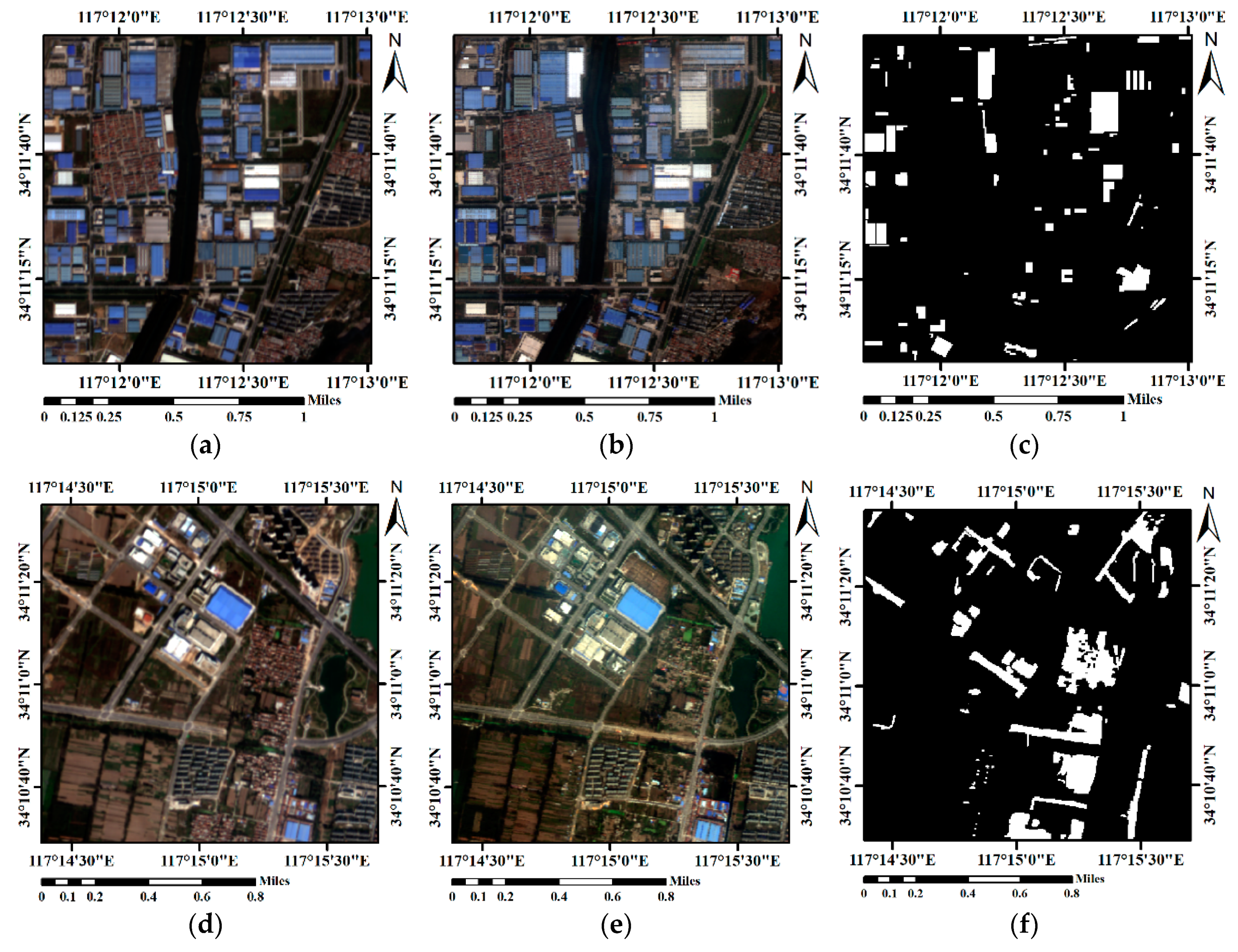
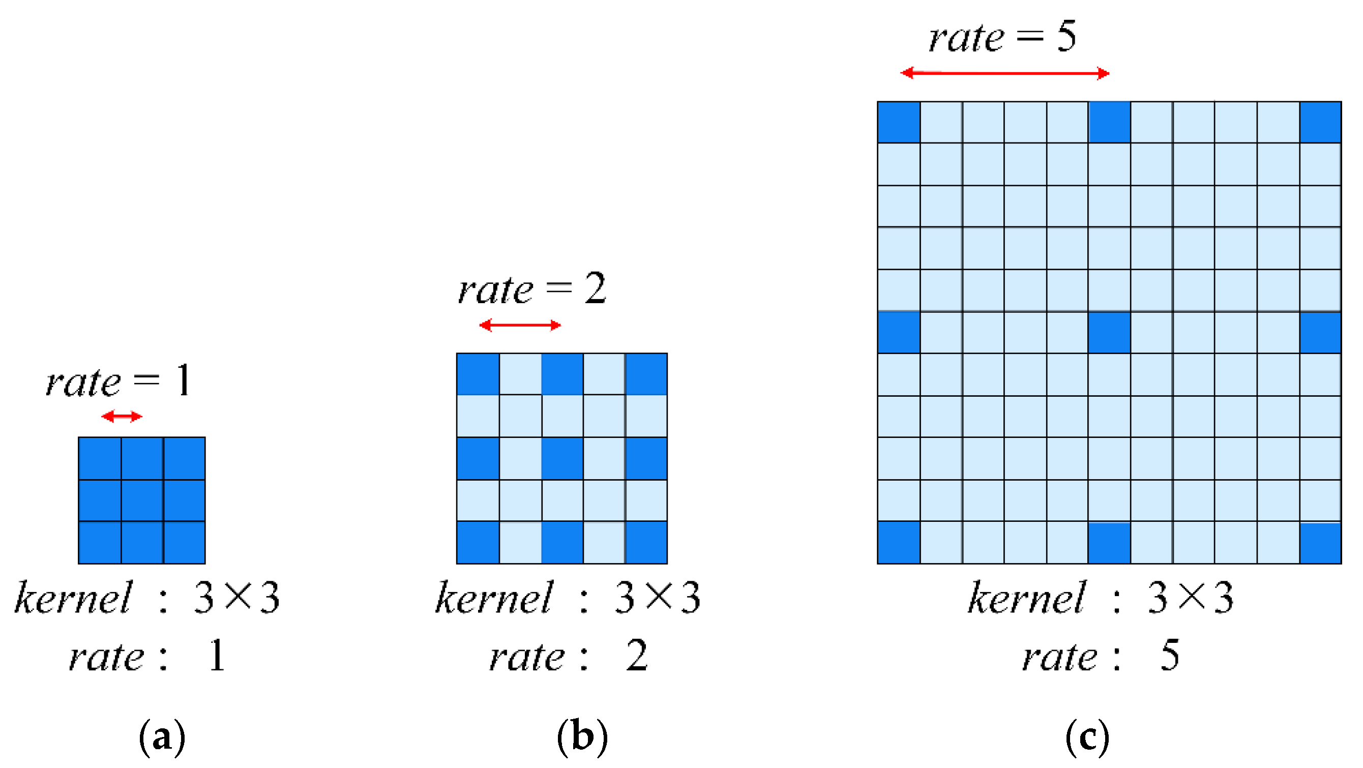
2.1. Data Description and Training Samples Acquisition

2.1.1. Data Description

In order to verify the effectiveness of the proposed method, the changes at three datasets are investigated. The first area covers part of Tongshan district, China, which are shown in Figure 1a,b, respectively. The second area is located near Dalong lake in Yunlong district, China, which are shown in Figure 1d–f, respectively. Figure 1g–h show the third area, which is located at Yunlong lake in Xuzhou, China. These three datasets represent three regions: Urban, rural-urban fringe, and non-urban areas. Date 1 is 1 October 2014 and the images were acquired by ZY-3 and date 2 is 5 October 2016 and the images were acquired by GF-2. The band combination of these three datasets is composed of blue, green, red, and near-infrared bands, with different resolutions and imaging conditions. Figure 1 shows the images and reference maps of these three datasets. The key technical specifications of ZY-3 and GF-2 satellites are shown in Table 1. Their sensors have presented challenges in change detection using multi-sensor data.
Both datasets were resampled to the same resolution of 5.8 m, and the geometric registration root-mean-square error (RMSE) is 0.5 pixels. The pseudo-invariant feature (PIF) was applied to achieve relative radiometric correction. The reference maps for both datasets were obtained via visual interpretation with the aid of prior knowledge and the images from Google Earth during the corresponding period, which are shown in Figure 1c,f,i.

2.1.2. Training Samples Acquisition

The manual selection of training samples is a time-consuming process and the selected samples often present incomplete representation. Therefore, the training samples are selected in combination with an automatic analysis process, based on differences in multi-feature images in this work.
Initial selection of changed and unchanged pixels is conducted by combining the individual detection results from spectral and texture features. Firstly, the Gabor features are constructed in the 0°, 45°, 90°, and 135°directions, with a kernel sizes of [7,9,11,13,15,17], for the transform-based texture features. Consider the original images with X spectral bands, the multi-kernel Gabor features in one direction is calculated as Equation (1),
G d i r e c t i o n x = k g k x ,           k [ 7 ,   9 ,   11 ,   13 ,   15 ,   17 ] ,
where g k x means the Gabor feature of x-th spectral band with a kernel size k. 4 × X Gabor features are then obtained.
The difference image D is generated from two temporal images, with the dataset consisting of the spectral features, and Gabor texture features. Consider the images with r spectral bands at t 1 and t 2 , D is calculated as follows:
D = | T 1 T 2 | .
Each dimension of D must be normalized in the range [0, 1], and data in the b-th dimensional D b is normalized as follows,
D b = D b D m i n D m a x D m i n ,   b = 1 , 2 , , r ,
where D m i n and D m a x are the minimum and maximum values of the difference image in b-th dimension. Equation (4) is aimed at obtaining the initial pixel-based change detection map C D b on each band,
c d i , j b = { 0 ,     i f   d i , j b < T b 1 ,     i f   d i , j b T b T b =   m b + s b ,   b = 1 , 2 , , r   ,
where c d i , j b indicates that the pixel at position ( i , j ) in C D b belongs to the unchanged or changed part. Tb is calculated according to the mean m b and standard deviation s b of the pixels on the b-th dimension. In order to select reliable training and testing samples, the uncertainty of each b-th dimensional difference image is considered, and a conservative decision is made as follows,
L i , j = { 0 ,   p 0.3 × b 1 ,       o t h e r w i s e p = r = 1 b c d i , j b     ,
where L i , j = 0 , 1 indicates that the label on position ( i , j ) in the image belongs to unchanged or changed part. p is the score that a pixel at position ( i , j ) considered to be changed by all dimensions.
For the pixel on position ( i , j ) , if the score p is greater than the threshold 0.7 × b , then the pixel will be labelled as “changed” category. Likewise, if p is less than 0.3 × b , then it will be labelled as “unchanged” category. Training samples were selected from these “certain” cases randomly. Patches of a fixed size ω centered on each selected pixel are taken as the input samples. Therefore, the inputs in our proposed methods are [ p a t c h 1 , p a t c h 2 , l a b e l ] .

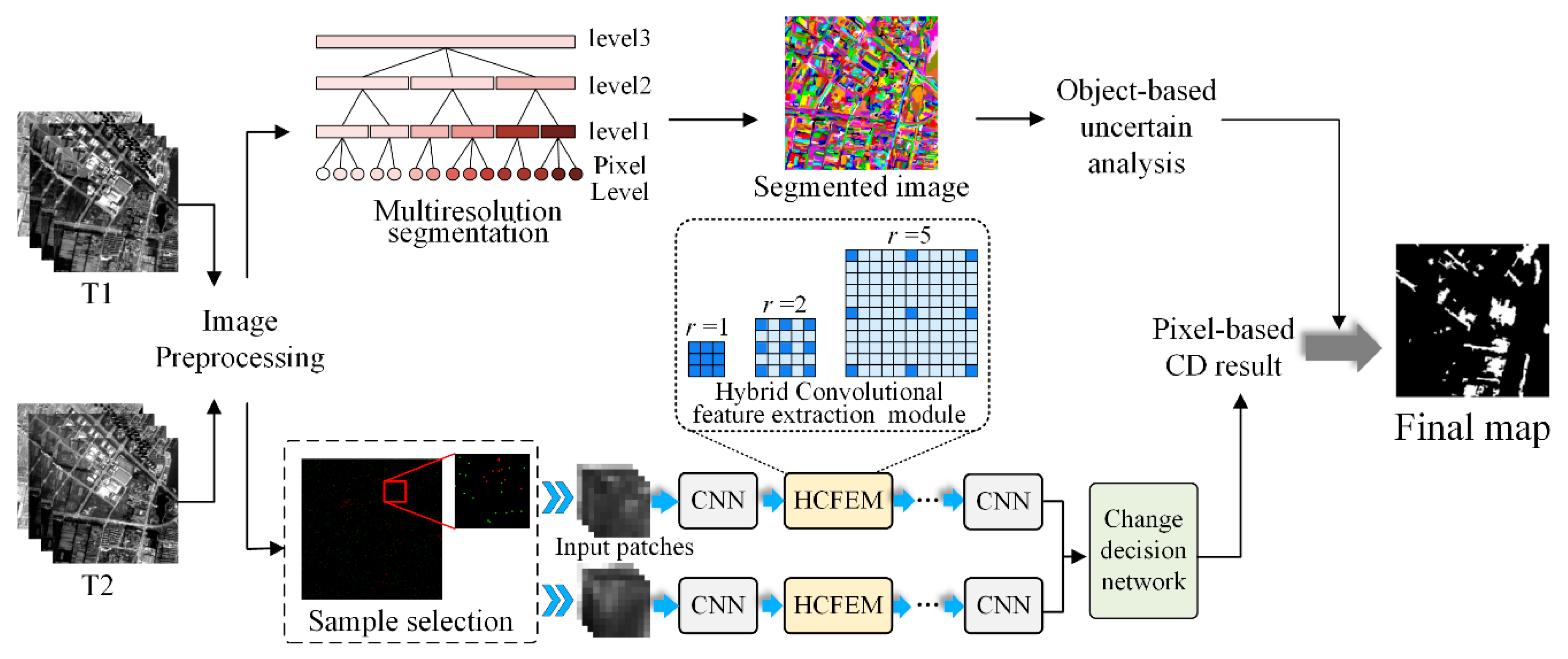
2.2. Proposed Approach

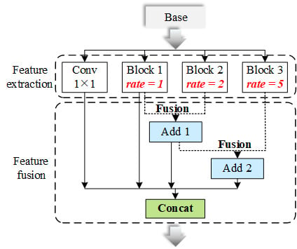
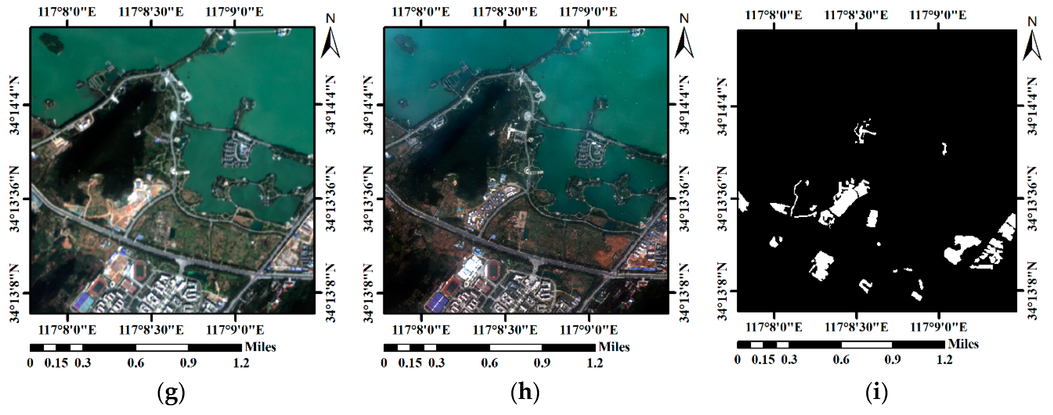
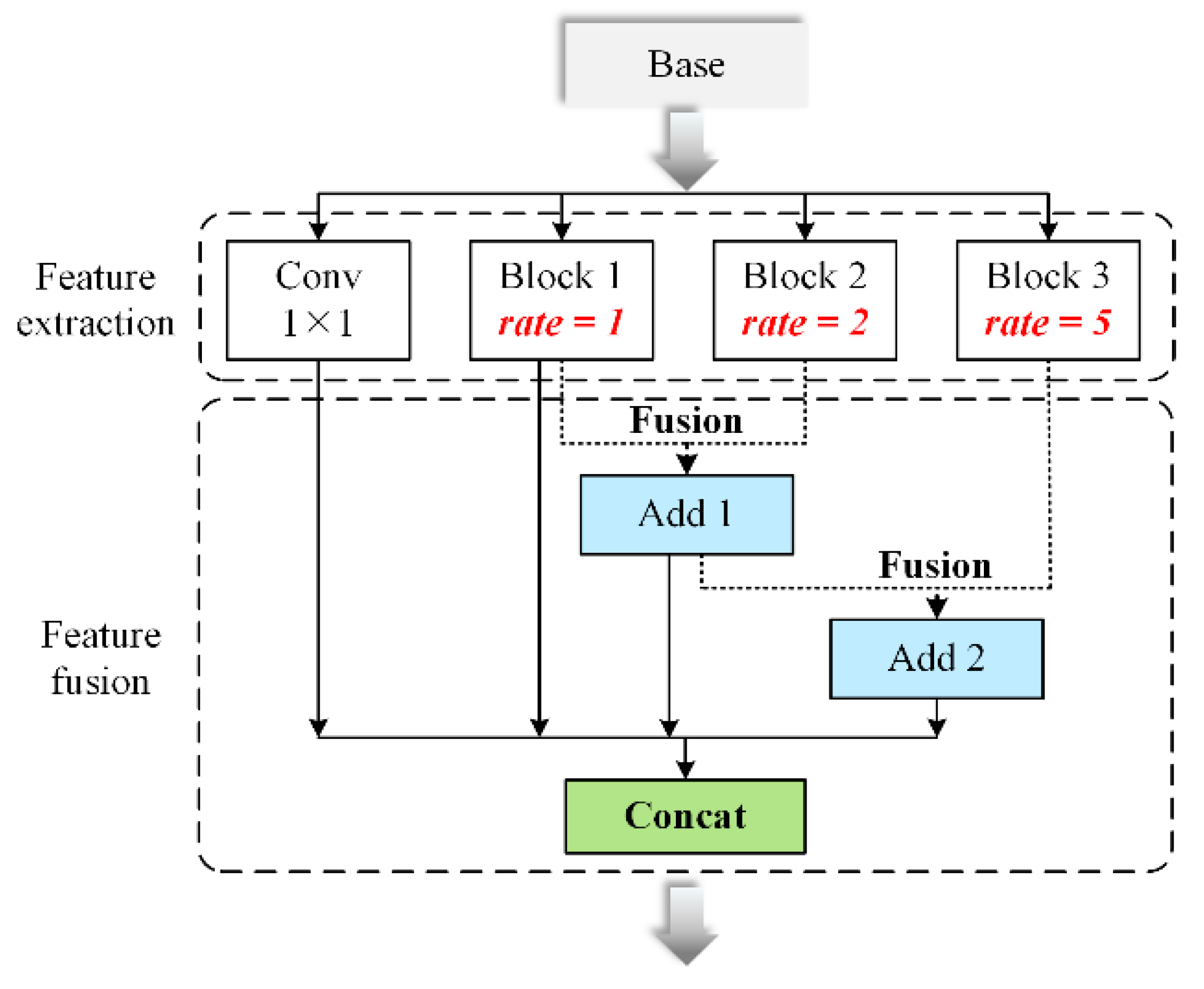
2.2.1. Hybrid Convolutional Feature Extraction Module

When an image patch is input into the model, such as FCN [40], it is firstly convolved and then pooled to reduce the size, and increase the receptive field at the same time. After that, the size of the patch is expanded by up-sampling and deconvolution operations. However, the pooling process gives rise to partial loss of image information. In this case, understanding how to achieve a larger receptive field without pooling has become a new question in the field of deep learning.
Dilated convolution (or Atrous convolution) was originally developed for wavelet decomposition [41], the main idea of which is to insert “holes” (zeros) between pixels in convolutional kernels to improve the resolution. The characteristic of expanding the receptive field without loss of resolution or coverage enables the deep CNNs to extract effective features [42]. As shown in Figure 2a, standard convolution, with kernel size 3 × 3, is equal to dilated convolution when rate = 1. Figure 2b illustrates the samples of dilated convolution when rate = 2. The receptive field is larger compared with the standard convolutional operation. Figure 2c shows the convolution with dilated convolution when rate = 5 and the receptive field reaches 11 × 11.
Before the architecture of Inception [35], further convolutional layers were stacked on top of each other, making the CNN deeper and deeper for the pursuit of better performance. The advent of Inception makes the structure of CNN wider and diverse. Based on the structure of “network in network”, the hybrid convolutional feature extraction module (HCFEM) is developed for the purpose of extracting effective features from the multi-sensor images in this work. As shown in Figure 3, HCFEM includes two units: Feature extraction unit and Feature fusion unit. Four channels with different convolutional operation compose the extraction unit: (1) 1 × 1 convolution kernel to increase nonlinearity of neural network and change the dimension of the image matrix; (2) block 1 uses convolutional layer with a dilation rate r = 1; (3) block 2 uses convolutional layer with a dilation rate r = 2; (4) block 3 uses convolutional layer with a dilation rate r = 5. Three blocks apply 3 × 3 convolutions. After the convolution operation by four channels, feature fusion is carried out. Add 1 refers to the fusion between the results from block 1 and block 2, and Add 2 refers to that between the results from Add 1 and block 3.
Based on dilated convolution and the structure of “network in network”, HCFEM can encode the object on multiple scales. With dilated convolution, deep convolutional neural network (DCNN) is able to control the resolution at which feature responses are computed, without requiring learning extra parameters [43]. Moreover, the “network in network” structure can increase the depth and width of the network, without any additional computational budget needed.

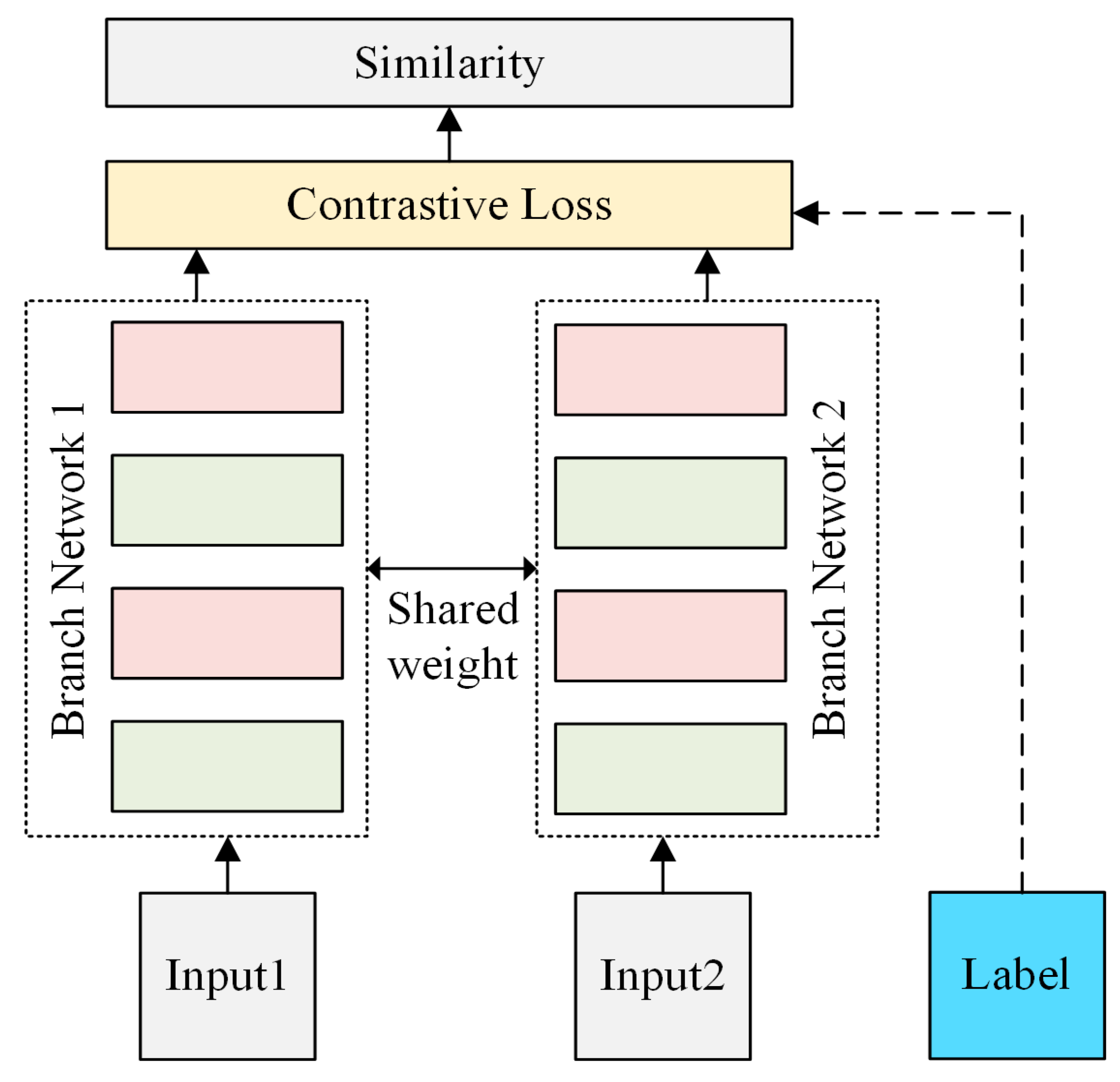
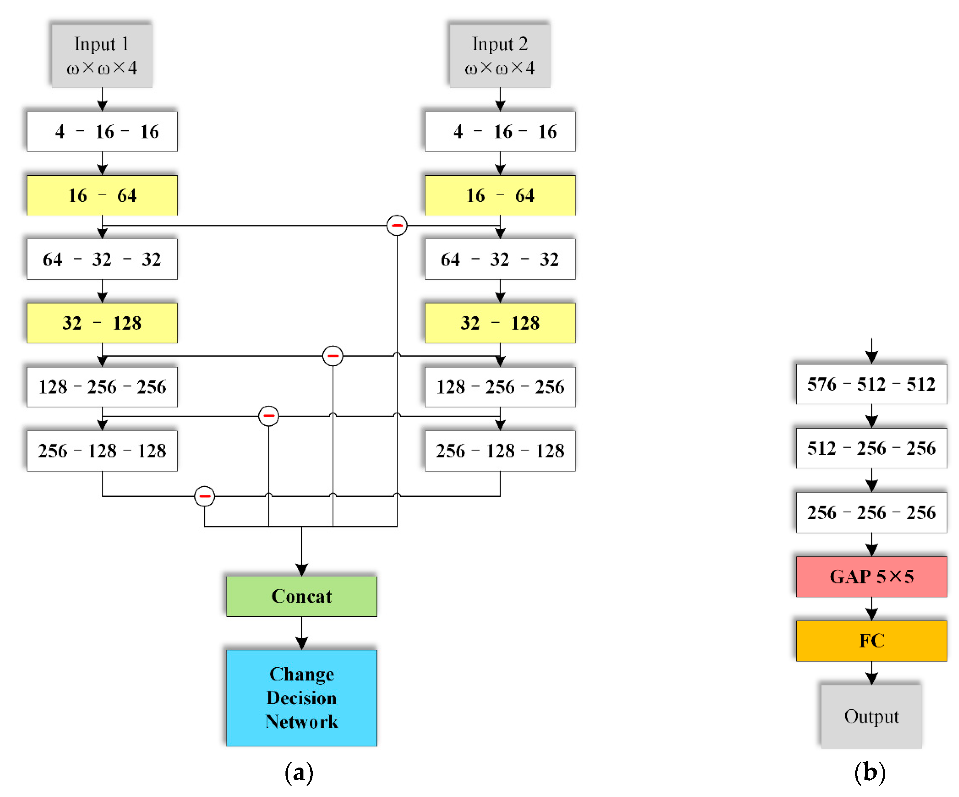
2.2.2. Network Architecture

Figure 4 shows a traditional Siamese neural network, which has two inputs and two branches. In Siamese neural network, two inputs feed into two neural networks (Network1 and Network2) concurrently and the similarity of the two inputs is evaluated by contrastive loss [44]. Based on the architecture of the Siamese network, a change decision approach has been proposed with Siamese convolutional neural network.
Combining with the architecture of “network in network”, we design a deep Siamese convolutional network based on HCFEM (DSCNH) for supervised change detection on multi-sensor images. The network consists of two components: Encoding network (feature extraction network) and change decision network. The layers in the encoding network are divided into two streams with same structure and shared weights as in a traditional Siamese network. As shown in Figure 5a, each image patch is inputted into these equal streams. Each stream is composed of heterogeneous convolution groups. In each group, the former convolutional module transforms the spatial and spectral measurements into high dimensional feature space, from which the subsequent HCFEM (colored in yellow in Figure 5) extracts the abundant features.
Through two heterogeneous convolution groups and another two normal convolutional modules, the absolute difference value of multiple-layer features are concatenated and inputted into the change decision network, in which three normal convolutional modules are used to extract difference features. A global average pooling layer (GAP) is carried out to decrease the number of parameters and avoid overfitting. The changed result is obtained after a fully connected layer. Figure 5a shows the designed deep Siamese convolutional neural network, and Figure 5b shows the change decision network.

2.2.3. Bootstrapping and Sampling Method for Training

To train the model properly with limited labelled samples, we introduce a sampling method based on the strategy of bootstrapping, which is implemented by constructing a number of resamples with replacement of the training samples [45]. Specifically, random sampling can be performed to extracting a certain number of samples, which are reused with new samples in the next iterative training process.

2.3. Multi-Resolution Segmentation

The images acquired by multiple sensors often present the great variations due to different imaging conditions, which brings strong noises in change detection. The object-oriented change detection (OBCD) can effectively restrain the influence of noise on change detection. Image segmentation is a primary step in OBCD, and the fractal net evolution approach (FNEA) is an effective and widely-used image segmentation method for remote sensing imagery [46]. It merges neighboring pixels with similar spectral measurements into a homogeneous image object following the principle of minimum average heterogeneity [47]. In the proposed method, two temporal images are combined into one data set by band stacking. The stacked image is then segmented on an over-segmented scale using FNEA. The segmented objects are then merged into multiple scales based on their heterogeneity.
In this work, the optimal segmentation scale S l according to the GS value is obtained firstly [18], then five segmentation scales, [ S l 2 ,   S l 1 ,   S l ,   S l + 1 ,   S l + 2 ], are selected. The optimal image segmentation scale, S l , is defined as the scale that maximizes the inter-segment heterogeneity and the intra-segment homogeneity [48]. The global Moran’s I [49], which calculates spatial autocorrelation, is used as the inter-segment heterogeneity measure, and is calculated as,
M I = n i = 1 n j = 1 n w i j ( y i y ¯ ) ( y j y ¯ ) ( i = 1 n ( y i y ¯ ) 2 ) ( i j w i j )
where w i j is the spatial adjacency measure of R i and R j . If regions R i and R j are neighbours,   w i j = 1 ; otherwise, w i j = 0 .   y i and y j are the mean values of   R i , and   R j , respectively. While,   y ¯ is the mean value of each band of the image. Low Moran’s I values indicate a low degree of spatial autocorrelation and high inter-segment heterogeneity.
The variance average weighted by each object area is used as the global intra-segment homogeneity measurement, which is calculated as,
V = i = 1 n a i v i i = 1 n a i
where a i and v i represent the area and variance of segment R i , respectively. n is the total number of objects in the segmentation map.
Both measurements are rescaled to range (0–1). To assign an overall “global score” (GS) on each segmentation scale, the V and M I are combined as the objective function:
G S = M I + V .
For each segmentation, the GSs are calculated on all the feature dimension. The average GS of all the feature bands are used to determine the best image segmentation scale, where the optimal segmentation scale is identified as the one with the lowest average GS value. For the experimental data, the segmentation scales of three datasets are set to [30,35,40,45,50], [25,30,35,40,45] and [25,30,35,40,45], respectively. The results on different segmentation scale are shown in Figure 6.

2.4. Change Detection Framework Combined with Deep Siamese Network and Multi-Resolution Segmentation

Patches of high-resolution remote sensing image are utilized in DSCNH to extract the deep context features and analyze the changes in the feature space. However, the learned spatial features are only restricted to a fixed neighborhood region. In this regard, we introduce the multi-resolution segmentation algorithm to fully explore the object’s spatial information. The pixel-based result obtained by DSCNH can be refined by an additional constraint in the same object, so as to make better use of the spatial information of multi sensor images.
Suppose the category ϑ = { C , U } , where C and U represent the changed and unchanged classes, respectively. Then the inputs are divided into these two categories through DSCNH, and the pixel-based change detection results can be obtained. For each scale level l, an object is represented as R i ,   i = 1 , 2 N , where N denotes the count of objects in level l , and threshold T is set to classify the objects R i using Equations (9) and (10).
C D i = { 1 ,     i f   p c > T   0 ,                   o t h e r s ,
p c =   j = 1 n n c j n ,
where p c represents the probability of object R i belonging to C in level l, n c j and n are the changed pixels and total number of pixels in object R i . If the C D i satisfies P c > T , the object R i is labeled as changed object. C D i = 0 ,   1 indicates that R i belongs to the unchanged and changed classes, respectively.
We can see now the proposed method can be regard as a combination with deep learning and multi-resolution segmentation (OB-DSCNH), including images pre-processing, sample selection, change detection based on DSCNH, and decision fusion. The flow chart of the procedures is shown in Figure 7.

3. Results

In order to demonstrate the effectiveness of the OB-DSCNH, two dates of images from two sensors were utilized at three locations. The factors that may impact the performance of the model were explored. The influence of different patch sizes was also studied, which is linked to the size of the receptive field. Five hundred changed, and one thousand unchanged, regions (patches) were chosen as the labelled dataset, fifty percent of which were randomly selected to be the training sets and the rest for testing. The threshold for the uncertainty analysis was set as 0.70 by trial and error. The segmentation scales of the three datasets were set as 40, 30, and 45, respectively, based on cross-validation. In this work, all the experiments were implemented in Python 3.7.

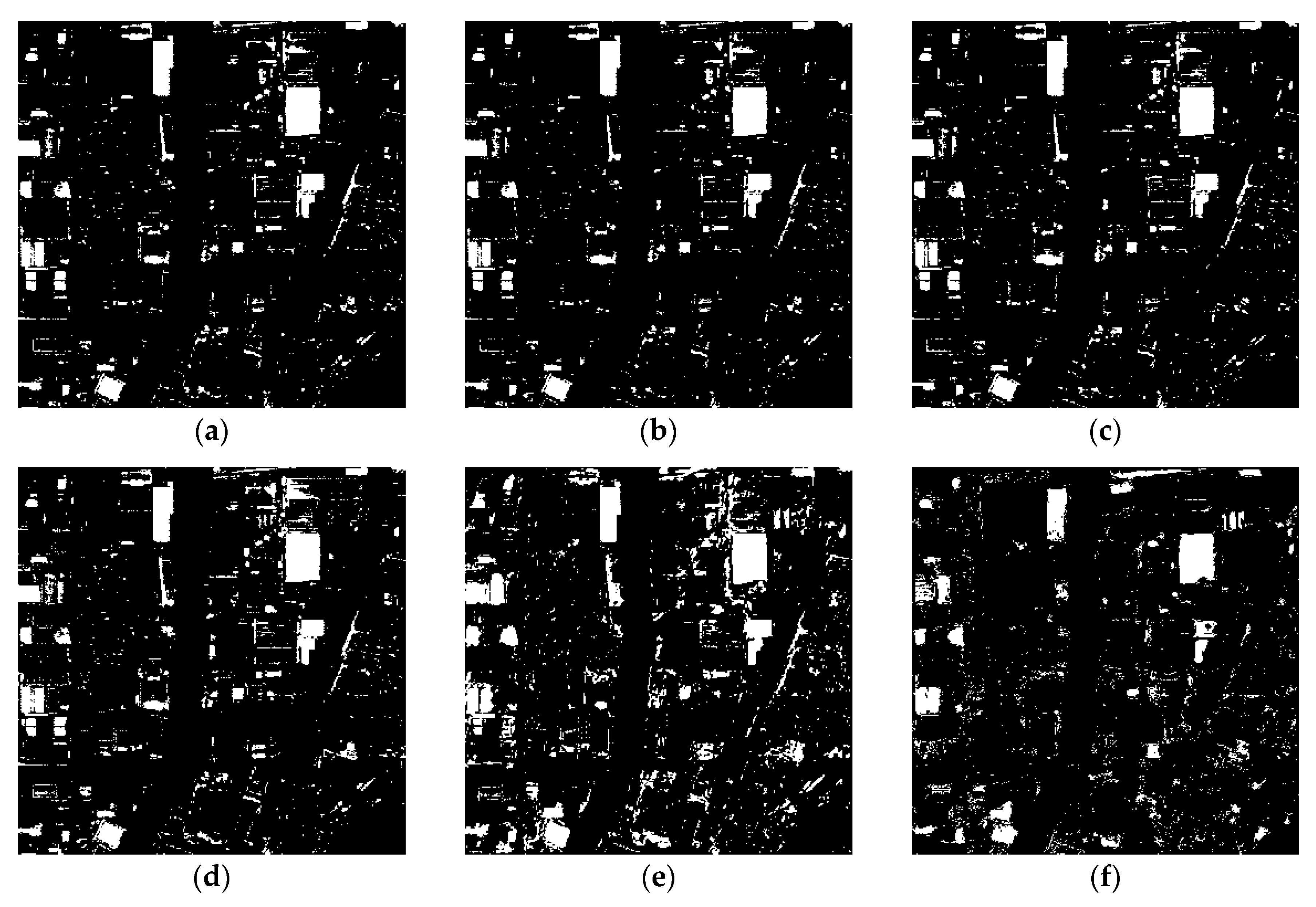
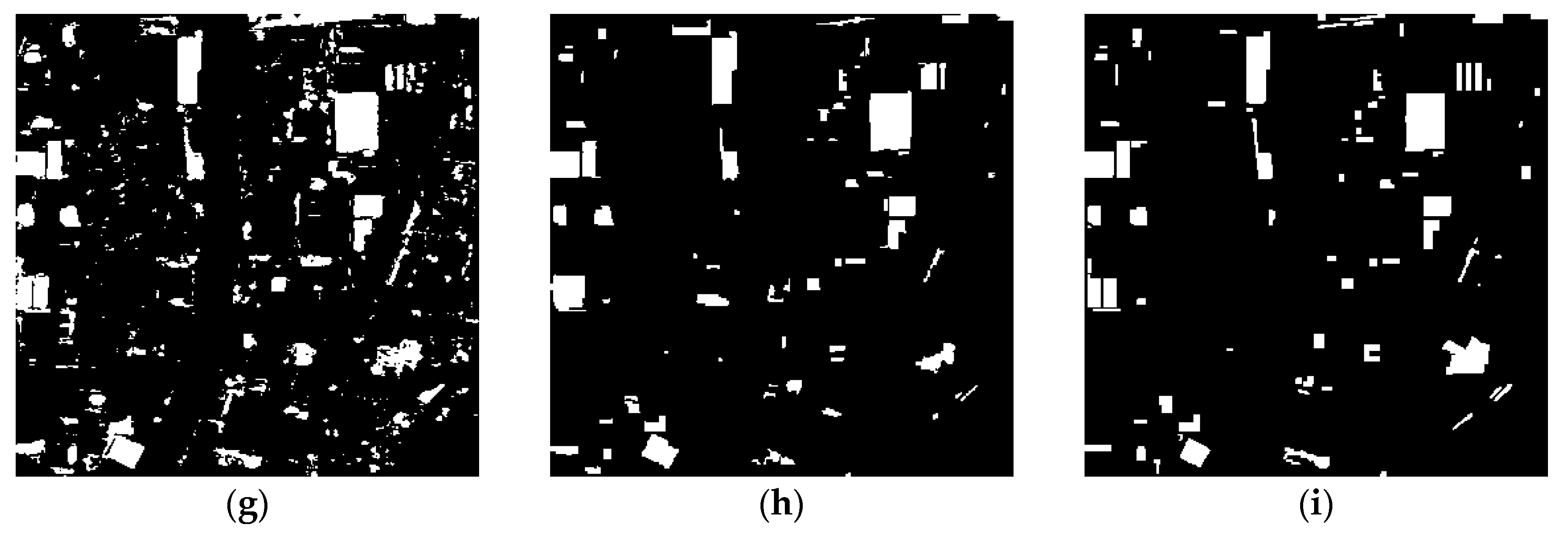
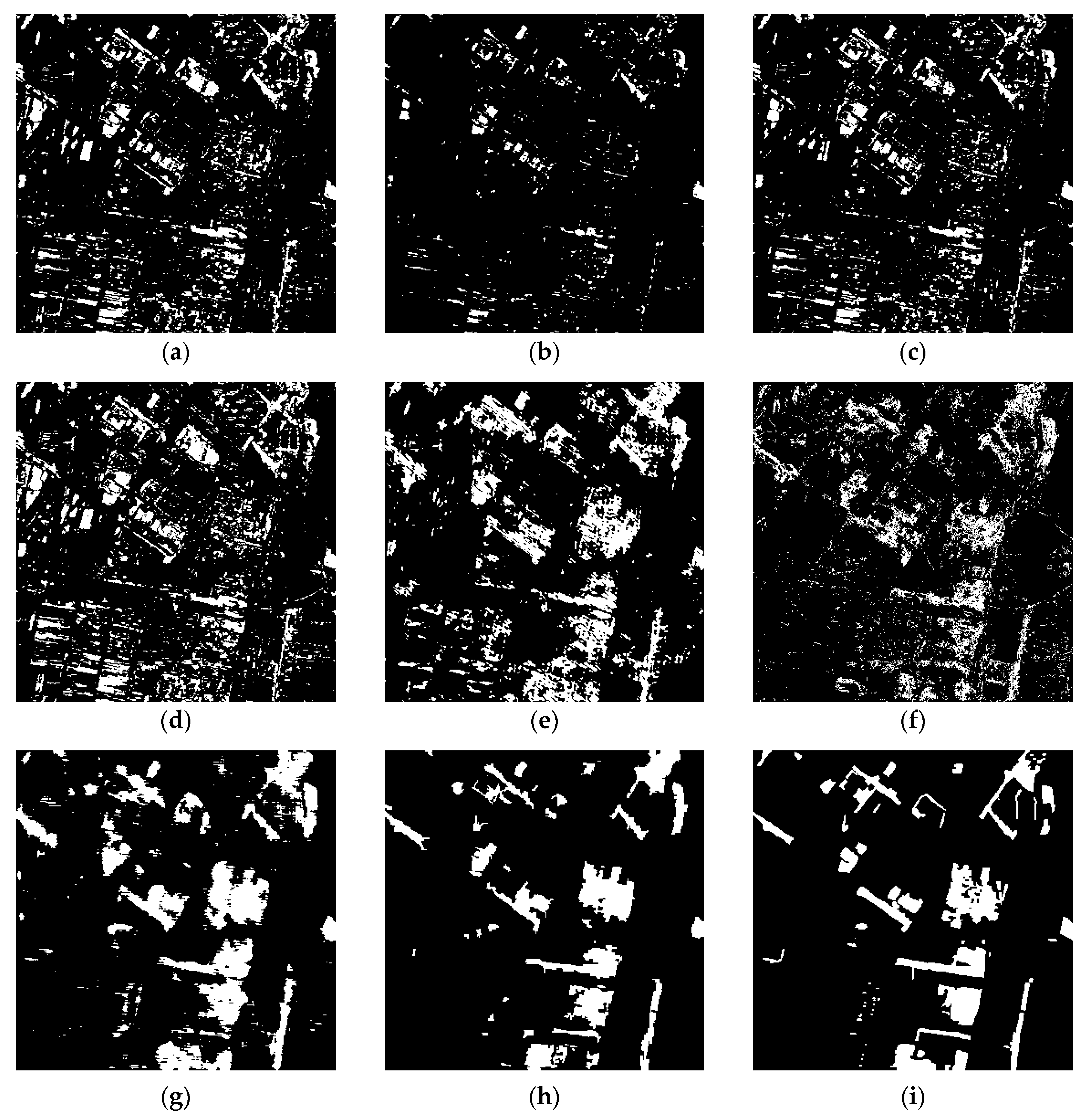
3.1. Experimental Results

We compared the proposed OB-DSCNH with the state-of-the-art methods to demonstrate its superiority. The supervised pixel-wise change detection methods of Multiple Linear Regression (MLR), Extreme Learning Machine (ELM), the Artificial Neural Network (ANN), and Support Vector Machine (SVM) were chosen as comparative methods. Moreover, CD based on the deep Siamese multi-scale convolutional network (DSMS-CN) [36], the deep convolutional neural network (DCNN), and traditional Siamese convolutional neural network (TSCNN) [25] were chosen on behalf of the deep learning methods in the contrast experiments. The patch size used in deep learning comparison experiments are the same as that of OB-DSCNH. The hyper-parameters of each method were chosen empirically.
Figure 8, Figure 9 and Figure 10 show the change detection results based on the deep Siamese convolutional network. The unchanged and changed classes are colored in black and white, respectively. It can be seen from the change maps that the changed regions in the first dataset mainly comprise the increased land and roads, and the decreased buildings. The changed regions in the last two datasets mainly are constructions. Compared with the reference change maps shown in Figure 8i, Figure 9i and Figure 10i, the change detection results of OB-DSCNH are more consistent with the reference change maps.
The detection results on the first dataset show that the change maps obtained by MLR, ELM, and SVM contain a large number of false detected pixels. From Figure 8d, ANN and the previous several methods present a similar result, which demonstrates the insufficiency of these classifiers on multi-sensor images. For the second dataset, there is a large area of cultivated land in the southwest of the image. The convention in change detection is that the area should be judged to be unchanged when it is covered by crops. As shown in Figure 9a–d, the common change detection methods fail to extract useful features towards the classification task, and there is significant “salt-and-pepper” noise due to the lack of spatial context usage. As shown in Figure 8e–h and Figure 9e–9h, deep convolutional neural networks have a powerful ability to extract spectral and spatial context information. The third dataset has less changes than the first two datasets. From Figure 10a–d, it can be seen clearly that the change maps, obtained by ELM, MLR, SVM, and ANN, contain many false detected pixels in the water area. OB-DSCAH and other deep learning methods succeed in the unchanged information detection, as shown in Figure 10e–h. Some of the “salt-and-pepper” noise in the change detection results is eliminated after including the segmented object information constraint.

3.2. Accuracy evaluation

In order to assess the performance of the proposed approach, four indicators are adopted by comparing the detection results with the ground truth: (1) Overall accuracy (OA); (2) Kappa coefficient; (3) commission error; and (4) omission error, which are defined as:
O A = ( N 11 + N 00 ) ( N 11 + N 00 + N 01 + N 10 ) K a p p a = N × ( N 11 + N 00 ) ( ( N 11 + N 10 ) × ( N 11 + N 01 ) + ( N 01 + N 00 ) × ( N 10 + N 00 ) ) N 2 ( ( N 11 + N 10 ) × ( N 11 + N 01 ) + ( N 01 + N 00 ) * ( N 10 + N 00 ) ) C o m m i s s i o n   e r r o r = N 01 ( N 01 + N 11 ) O m i s s i o n   e r r o r = N 10 ( N 10 + N 00 )
where N 11 and N 00 are the numbers of changed pixels and unchanged pixels correctly detected, respectively; N 10 denotes the number of missed changed pixels; N 01 is the number of unchanged pixels in the ground reference that are detected as changed in the change map; and N is the total number of the labelled pixels.
The accuracies of the change detection for the three datasets are listed in Table 2, Table 3 and Table 4. It can be clearly seen that the proposed OB-DSCNH obtains a higher change detection accuracy than the other methods. The accuracy of OB-DSCNH achieves the highest among all the methods with the OAs being 0.9715, 0.9468, and 0.9792 on the three datasets. In the first dataset, the OA of OB-DSCNH is superior to DSMS-CN by 3.24%, and the Kappa coefficient is superior by 13%. The OA and Kappa of OB-DSCNH are increased by 2.21%, 5% on the second dataset compared with which of DSMS-CN, respectively. On the third dataset, the OA of OB-DSCNH are superior to other deep learning methods by more than 2.9%, and the Kappa coefficient is increased by 16.6% compared with which of DSMS-CN. These results demonstrate the superiority in effectiveness and the generalizability of the proposed method.
Atmosphere and illumination variations may lead to the complicated feature statistics for the multi-sensor images, resulting in poor performance on change detection for some classical methods. It is evident that the proposed method can extract the deep and separable features from the training data towards change detection task. OB-DSCNH outperforms the classical methods, such as SVM and ELM, which can be ascribed to the extracted features by the deep Siamese convolutional network. Although, the omission error is higher than DSMS-CN, the proposed method still presents a stronger robustness compared with DSMS-CN on the three datasets.

4. Discussion

In the proposed network, the input consists of a pair of satellite images with an alterable size. To detect the changes of landcover using fine-grained features, the size of the input patch needs to be considered carefully. In this study, five sizes of input patch are chosen to analyze the influence on the accuracy. The values of three datasets are set to [5,7,9,11,13], [7,9,11,13,15], and [5,7,9,11,13] respectively. The experimental results in this part are obtained without constraining by segmentation, in order to eliminate the influence of the segmentation scale.
The accuracies under different patch sizes for change detection are listed in Table 5, Table 6 and Table 7. It can be seen that, for the first dataset, the model yields the highest OA when patch size is 5 while the omission ratio is also higher than others. The aggregative indicators show that the optimum is 7. For the second dataset, the method achieves the best performance when the patch size is 13. When the patch size is 9, the method preforms best on the third dataset.
Generally, most of the changes come from buildings in the first dataset. Relatively, a single change category and regular change shape should be the main reason that caused the patch size has no significant impact on the accuracy on the first dataset. As is shown in Table 5, due to the complexity of surface feature in the second dataset, the accuracy of change detection is improved obviously when the patch size changes from 7 to 13. Compared to the first dataset, change scenarios in this area are more complex, such as a large number of buildings being demolished and turned into land. If the patch size is too small, the network cannot fully learn the change information of surface feature, as well as its surrounding areas, which results in the inability to accurately detect these changes.

5. Conclusions

In this paper, we propose a supervised change detection method based on the deep Siamese convolutional network for multi-sensor images. The hybrid convolutional feature extraction module (HCFEM) has been designed based on dilated convolution and the structure of “network in network”. The proposed method is capable of extracting the hierarchical features from the input image pairs, which are more abstract and robust than comparative methods. In order to demonstrate the performance of the proposed technique, two multi-sensor datasets at three locations were utilized. Experimental results demonstrate that the proposed method achieves significant superiority than mainstream methods in multi-sensor images change detection.
However, when the central pixel and its neighborhoods are not in the same category, they are still regarded as the same class because of the impartible of the square input patch, which is the limitation of OB-DSCNH. In future work, segmentation object, taken as a training sample, will be explored. In addition, the unsupervised representation learning methods will also be considered during the detection process.

Author Contributions

K.T. and M.W. conceived and designed the experiments. M.W. performed the experiments and analyzed the results. K.T. and M.W. wrote the manuscript. X.J., X.W., and Y.C. gave comments and suggestions on the manuscript and proofread the document. All authors have read and agreed to the published version of the manuscript.

Funding

This research is supported in part by Natural Science Foundation of China (No. 41871337) and Priority Academic Program Development of Jiangsu Higher Education Institutions.

Conflicts of Interest

The authors declare no conflict of interest.

References

  1. Singh, A. Digital Change Detection Techniques Using Remotely Sensed Data. Int. J. Remote Sens. 1988, 10, 989–1003. [Google Scholar] [CrossRef] [Green Version]
  2. Mubea, K.; Menz, G. Monitoring Land-Use Change in Nakuru (Kenya) Using Multi-Sensor Satellite Data. Adv. Remote Sens. 2012, 1, 74–84. [Google Scholar] [CrossRef] [Green Version]
  3. Chen, Y.; He, X.; Wang, J.; Xiao, R. The Influence of Polarimetric Parameters and an Object-Based Approach on Land Cover Classification in Coastal Wetlands. Remote Sens. 2014, 6, 12575–12592. [Google Scholar] [CrossRef] [Green Version]
  4. Brunner, D.; Lemoine, G.; Bruzzone, L. Earthquake Damage Assessment of Buildings Using VHR Optical and SAR Imagery. IEEE Trans. Geosci. Remote Sens. 2010, 48, 2403–2420. [Google Scholar] [CrossRef] [Green Version]
  5. Lu, D.; Mausel, P.; Brondizio, E.; Moran, E. Change Detection Techniques. Int. J. Remote Sens. 2004, 25, 2365–2407. [Google Scholar] [CrossRef]
  6. Volpi, M.; Tuia, D.; Bovolo, F.; Kanevski, M.; Bruzzone, L. Supervised Change Detection in VHR Images Using Contextual Information and Support Vector Machines. Int. J. Appl. Earth Obs. Geoinf. 2013, 20, 77–85. [Google Scholar] [CrossRef]
  7. Huang, G.B.; Zhu, Q.Y.; Siew, C.K. Extreme Learning Machine: A New Learning Scheme of Feedforward Neural Networks. In Proceedings of the IEEE International Joint Conference on Neural Networks, Budapest, Hungary, 25–29 July 2004; pp. 985–990. [Google Scholar]
  8. Bachtiar, L.R.; Unsworth, C.P.; Newcomb, R.D.; Crampin, E.J. Multilayer Perceptron Classification of Unknown Volatile Chemicals from the Firing Rates of Insect Olfactory Sensory Neurons and Its Application to Biosensor Design. Neural Comput. 2013, 25, 259–287. [Google Scholar] [CrossRef]
  9. Song, X.; Cheng, B. Change Detection Using Change Vector Analysis from Landsat TM Images in Wuhan. Procedia Environ. Sci. 2011, 11, 238–244. [Google Scholar]
  10. Huo, C.; Zhou, Z.; Lu, H.; Pan, C.; Chen, K. Fast Object-Level Change Detection for VHR Images. IEEE Geosci. Remote Sens. Lett. 2010, 7, 118–122. [Google Scholar] [CrossRef]
  11. Hao, M.; Zhang, H.; Shi, W.; Deng, K. Unsupervised Change Detection Using Fuzzy C-means and MRF From Remotely Sensed Images. Remote Sens. Lett. 2013, 4, 1185–1194. [Google Scholar] [CrossRef]
  12. Moser, G.; Angiati, E.; Serpico, S.B. Multiscale Unsupervised Change Detection on Optical Images by Markov Random Fields and Wavelets. IEEE Geosci. Remote Sens. Lett. 2011, 8, 725–729. [Google Scholar] [CrossRef]
  13. Chen, Q.; Chen, Y. Multi-Feature Object-Based Change Detection Using Self-Adaptive Weight Change Vector Analysis. Remote Sens. 2016, 8, 549. [Google Scholar] [CrossRef] [Green Version]
  14. Huang, X.; Wen, D.; Li, J.; Qin, R. Multi-Level Monitoring of Subtle Urban Changes for The Megacities of China Using High-Resolution Multi-view Satellite Imagery. Remote Sens. Environ. 2017, 196, 56–75. [Google Scholar] [CrossRef]
  15. Blaschke, T. Object Based Image Analysis for Remote Sensing. ISPRS J. Photogramm. Remote Sens. 2010, 65, 2–16. [Google Scholar] [CrossRef] [Green Version]
  16. Tang, Y.; Zhang, L.; Huang, X. Object-oriented Change Detection Based on the Kolmogorov-Smirnov Test Using High-Resolution Multispectral Imagery. Int. J. Remote Sens. 2011, 32, 5719–5740. [Google Scholar] [CrossRef]
  17. Li, L.; Li, X.; Zhang, Y.; Wang, L.; Ying, G. Change Detection for High-resolution Remote Sensing Imagery Using Object-Oriented Change Vector Aanalysis Method. In Proceedings of the IEEE International Geoscience and Remote Sensing Symposium, Beijing, China, 10–15 July 2016; pp. 2873–2876. [Google Scholar]
  18. Tan, K.; Zhang, Y.; Wang, X.; Chen, Y. Object-Based Change Detection Using Multiple Classifiers and Multi-Scale Uncertainty Analysis. Remote Sens. 2019, 11, 359. [Google Scholar] [CrossRef] [Green Version]
  19. Wu, X.; Zhu, X.; Wu, G.Q.; Ding, W. Data Mining With Big Data. IEEE Trans. Knowl. Data Eng. 2014, 26, 97–107. [Google Scholar] [CrossRef]
  20. Baltrusaitis, T.; Ahuja, C.; Morency, L.-P. Multimodal Machine Learning: A Survey and Taxonomy. IEEE Trans. Pattern Anal. Mach. Intell. 2019, 41, 423–443. [Google Scholar] [CrossRef] [Green Version]
  21. Lahat, D.; Adali, T.; Jutten, C. Multimodal Data Fusion: An Overview of Methods, Challenges, and Prospects. Proc. IEEE 2015, 103, 1449–1477. [Google Scholar] [CrossRef] [Green Version]
  22. Ramachandram, D.; Taylor, G.W. Deep Multimodal Learning A Survey on Recent Advances and Trends. IEEE Signal Process. Mag. 2017, 34, 96–108. [Google Scholar] [CrossRef]
  23. Srivastava, N.; Salakhutdinov, R. Multimodal Learning with Deep Boltzmann Machines. J. Mach. Learn. Res. 2014, 15, 2949–2980. [Google Scholar]
  24. Zhao, W.; Wang, Z.; Gong, M.; Liu, J. Discriminative Feature Learning for Unsupervised Change Detection in Heterogeneous Images Based on a Coupled Neural Network. IEEE Trans. Geosci. Remote Sens. 2017, 55, 7066–7080. [Google Scholar] [CrossRef]
  25. Zhan, Y.; Fu, K.; Yan, M.; Sun, X.; Wang, H.; Qiu, X. Change Detection Based on Deep Siamese Convolutional Network for Optical Aerial Images. IEEE Geosci. Remote Sens. Lett. 2017, 14, 1845–1849. [Google Scholar] [CrossRef]
  26. Mercier, G.; Moser, G.; Serpico, S.B. Conditional Copulas for Change Detection in Heterogeneous Remote Sensing Images. IEEE Trans. Geosci. Remote Sens. 2014, 46, 1428–1441. [Google Scholar] [CrossRef]
  27. Prendes, J.; Chabert, M.; Pascal, F.; Giros, A.; Tourneret, J.-Y. A New Multivariate Statistical Model for Change Detection in Images Acquired by Homogeneous and Heterogeneous Sensors. IEEE Trans. Image Process. 2015, 24, 799–812. [Google Scholar] [CrossRef] [PubMed] [Green Version]
  28. Touati, R.; Mignotte, M.; Dahmane, M. A Reliable Mixed-Norm-Based Multiresolution Change Detector in Heterogeneous Remote Sensing Images. IEEE J. Sel. Top. Appl. Earth Obs. Remote Sens. 2019, 12, 3588–3601. [Google Scholar] [CrossRef]
  29. Wang, X.; Tan, K.; Du, Q.; Chen, Y.; Du, P. Caps-TripleGAN: GAN-Assisted CapsNet for Hyperspectral Image Classification. IEEE Trans. Geosci. Remote Sens. 2019, 57, 7232–7245. [Google Scholar] [CrossRef]
  30. Tan, K.; Wu, F.; Du, Q.; Du, P.; Chen, Y. A Parallel Gaussian–Bernoulli Restricted Boltzmann Machine for Mining Area Classification With Hyperspectral Imagery. IEEE J. Sel. Top. Appl. Earth Obs. Remote Sens. 2019, 12, 627–636. [Google Scholar] [CrossRef]
  31. Hinton, G.E.; Osindero, S.; Teh, Y.-W. A Fast Learning Algorithm for Deep Belief Nets. Neural Comput. 2006, 18, 1527–1554. [Google Scholar] [CrossRef]
  32. Vincent, P.; Larochelle, H.; Lajoie, I.; Bengio, Y.; Manzagol, P.-A. Stacked Denoising Autoencoders: Learning Useful Representations in a Deep Network with a Local Denoising Criterion. J. Mach. Learn. Res. 2010, 11, 3371–3408. [Google Scholar]
  33. Hu, B.; Lu, Z.; Li, H.; Chen, Q. Convolutional Neural Network Architectures for Matching Natural Language Sentences. In Advances in Neural Information Processing Systems; NIPS Foundation, Inc.: San Diego, CA, USA, 2014; Volume 27. [Google Scholar]
  34. Simonyan, K.; Zisserman, A. Very Deep Convolutional Networks for Large-Scale Image Recognition. arXiv 2015, arXiv:1409.1556. [Google Scholar]
  35. Szegedy, C.; Liu, W.; Jia, Y.; Sermanet, P.; Reed, S.; Anguelov, D.; Erhan, D.; Vanhoucke, V.; Rabinovich, A. Going Deeper with Convolutions. In Proceedings of the IEEE Conference on Computer Vision and Pattern Recognition, Columbus, OH, USA, 24–27 June 2014; pp. 1–9. [Google Scholar]
  36. He, K.; Zhang, X.; Ren, S.; Sun, J. Deep Residual Learning for Image Recognition. In Proceedings of the IEEE Conference on Computer Vision and Pattern Recognition, Boston, MA, USA, 7–12 June 2015; pp. 770–778. [Google Scholar]
  37. Daudt, R.C.; Le Saux, B.; Boulch, A. Fully Convolutional Siamese Networks for Change Detection. In Proceedings of the 2018 25th IEEE International Conference on Image Processing, Athens, Greece, 7–10 October 2018; Volume 36, pp. 4063–4067. [Google Scholar]
  38. Chen, H.; Wu, C.; Du, B.; Zhang, L. Deep Siamese Multi-scale Convolutional Network for Change Detection in Multi-temporal VHR Images. arXiv 2019, arXiv:1906.11479. [Google Scholar]
  39. Liu, J.; Gong, M.; Qin, K.; Zhang, P. A Deep Convolutional Coupling Network for Change Detection Based on Heterogeneous Optical and Radar Images. IEEE Trans. Neural Netw. Learn. Syst. 2018, 29, 545–559. [Google Scholar] [CrossRef] [PubMed]
  40. Long, J.; Shelhamer, E.; Darrell, T. Fully Convolutional Networks for Semantic Segmentation. In Proceedings of the 2015 IEEE Conference on Computer Vision and Pattern Recognition (CVPR), Boston, MA, USA, 7–12 June 2015; Volume, 39, pp. 640–651. [Google Scholar]
  41. Holschneider, M.; Kronland-Martinet, R.; Morlet, J.; Tchamitchian, P. A Real-Time Algorithm for Signal Analysis with the Help of the Wavelet Transform. In Wavelets; Springer: Berlin/Heidelberg, Germany, 1989; pp. 286–297. [Google Scholar]
  42. Wang, P.; Chen, P.; Yuan, Y.; Liu, D.; Huang, Z.; Hou, X.; Cottrell, G. Understanding Convolution for Semantic Segmentation. In Proceedings of the IEEE Winter Conference on Applications of Computer Vision, Lake Tahoe, NV, USA, 12–15 March 2018; pp. 1451–1460. [Google Scholar]
  43. Chen, L.-C.; Papandreou, G.; Schroff, F.; Adam, H. Rethinking Atrous Convolution for Semantic Image Segmentation. arXiv 2017, arXiv:1706.05587. [Google Scholar]
  44. Chopra, S.; Hadsell, R.; LeCun, Y. Learning A Similarity Metric Discriminatively, with Application to Face Verification. In Proceedings of the 2005 IEEE Computer Society Conference on Computer Vision and Pattern Recognition (CVPR’05), San Diego, CA, USA, 20–25 June 2005; pp. 539–546. [Google Scholar]
  45. Rahman, F.; Vasu, B.; Van Cor, J.; Kerekes, J.; Savakis, A. Siamese Network with Multi-Level Features for Patch-Based Change Detection in Satellite Imagery. In Proceedings of the 2018 IEEE Global Conference on Signal and Information Processing, Anaheim, CA, USA, 26–29 November 2018; pp. 958–962. [Google Scholar]
  46. Hay, G.J.; Blaschke, T.; Marceau, D.J.; Bouchard, A. A Comparison of Three Image-Object Methods for The Multiscale Analysis of Landscape Structure. ISPRS J. Photogramm. Remote Sens. 2003, 57, 327–345. [Google Scholar] [CrossRef]
  47. Zhang, X.; Du, S. Learning Selfhood Scales for Urban Land Cover Mapping with Very-High-Resolution Satellite Images. Remote Sens. Environ. 2016, 178, 172–190. [Google Scholar] [CrossRef]
  48. Lu, Q.; Ma, Y.; Xia, G.-S. Active Learning for Training Sample Selection in Remote Sensing Image Classification Using Spatial Information. Remote Sens. Lett. 2017, 8, 1211–1220. [Google Scholar] [CrossRef]
  49. Espindola, G.M.; Camara, G.; Reis, I.A.; Bins, L.S.; Monteiro, A.M. Parameter Selection for Region-Growing Image Segmentation Algorithms Using Spatial Autocorrelation. Int. J. Remote Sens. 2006, 27, 3035–3040. [Google Scholar] [CrossRef]
Figure 1. True-color images and reference change maps of the three datasets. (a,b) True-color images in the first dataset. (c) Reference change map of the first dataset. (d,e) True-color images in the second dataset. (f) Reference change map of the second dataset. (g,h) True-color images in the third dataset. (i) Reference change map of the third dataset. (a,d,g) are ZY-3 satellite images. (b,e,h) are GF-2 satellite images.
Remotesensing 12 00205 g001aRemotesensing 12 00205 g001b
Figure 2. Illustration of the dilated convolution. (a) dilated convolution layer when rate = 1. (b) dilated convolution layer when rate = 2. (c) dilated convolution layer when rate = 5.
Remotesensing 12 00205 g002
Figure 3. Illustration of the designed Siamese architectures for change detection. Hybrid convolutional feature extraction module (HCFEM), including: (1) Feature extraction unit. (2) Feature fusion unit.
Remotesensing 12 00205 g003
Figure 4. Illustration of a traditional Siamese network structure.
Remotesensing 12 00205 g004
Figure 5. Illustration of the designed Siamese architectures for change detection. (a) Schematics of the proposed architectures (DSCNH). (b) Architecture of change decision network. Block color legend: White means normal convolution with kernel size 3 × 3, yellow means the proposed HCFEM, green means concatenation, blue means the Change Decision Network, red means Global Average Pooling layer, and orange means Fully Connected layer.
Remotesensing 12 00205 g005
Figure 6. Illustration of several objects of images in data after multi-resolution segmentation by fractal net evolution approach (FNEA). Segmentation scales on the first location are set as (a) 30, (b) 35, (c) 40, (d) 45, (e) 50, respectively. Segmentation scales on the second location are set as (f) 25, (g) 30, (h) 35, (i) 40, (j) 45, respectively. Segmentation scales on the third location are set as (k) 25, (l) 30, (m) 35, (n) 40, (o) 45, respectively.
Remotesensing 12 00205 g006
Figure 7. The flow chart of proposed method.
Remotesensing 12 00205 g007
Figure 8. Change detection maps obtained on the first location by: (a) Extreme Learning Machine ELM, (b) Support Vector Machine (SVM), (c) Multiple Linear Regression (MLR), (d) Artificial Neural Network (ANN), (e) Deep Convolutional Neural Network (DCNN) (ω = 7), (f) Traditional Siamese Convolutional Neural Network (TSCNN) (ω = 7), (g) Deep Siamese Multi-Scale Convolutional Network (DSMS-CN) (ω = 7), (h) Deep Siamese Convolutional Network based on Convolutional Feature Extraction Module (OB-DSCNH) (ω = 7, l =40), (i) Reference map.
Remotesensing 12 00205 g008aRemotesensing 12 00205 g008b
Figure 9. Change detection maps obtained on the second location by: (a) Extreme Learning Machine (ELM), (b) Support Vector Machine (SVM), (c) Multiple Linear Regression (MLR), (d) Artificial Neural Network (ANN), (e) Deep Convolutional Neural Network (DCNN) (ω = 13), (f) Traditional Siamese Convolutional Neural Network (TSCNN) (ω = 13), (g) Deep Siamese Multi-scale Convolutional Network (DSMS-CN) (ω = 13), (h) Deep Siamese Convolutional Network Based on Convolutional Feature Extraction Module (OB-DSCNH) (ω = 13, l = 30), (i) Reference map.
Remotesensing 12 00205 g009
Figure 10. Change detection maps obtained on the third location by: (a) Extreme Learning Machine (ELM), (b) Support Vector Machine (SVM), (c) Multiple Linear Regression (MLR), (d) Artificial Neural Network (ANN), (e) Deep Convolutional Neural Network (DCNN) (ω = 9), (f) Traditional Siamese Convolutional Neural Network (TSCNN) (ω = 9), (g) Deep Siamese Multi-Scale Convolutional Network (DSMS-CN) (ω = 9), (h) Deep Siamese Convolutional Network Based on Convolutional Feature Extraction Module (OB-DSCNH) (ω = 9, l = 45), (i) Reference map.
Remotesensing 12 00205 g010
Table 1. Information of ZY-3 and GF-2 images used in this study.
SatellitePayloadBandSpectrum Range
(μm)
Spatial Resolution
(m)
Time
ZY-3MUXBlue0.45~0.525.82014.10.14
Green0.52~0.59
Red0.63~0.69
Nir0.77~0.89
GF-2PMSBlue0.45~0.5242016.10.05
Green0.52~0.59
Red0.63~0.69
Nir0.77~0.89
Table 2. Accuracy of the different change detection methods on the first dataset.
MethodOAKappaCommissionOmission
MLR0.94130.58020.42420.3474
ELM0.94470.60330.40220.3270
SVM0.94700.60970.38170.3405
ANN0.93780.58500.45280.2895
DCNN0.9268 0.5805 0.5094 0.1655
TSCNN0.9382 0.5544 0.4421 0.3791
DSMS-CN0.93910.64590.45730.0998
OB-DSCNH
(ω = 7, l = 40)
0.97150.78010.18940.2193
* The best results are shown in bold.
Table 3. Accuracy of the different change detection methods on the second dataset.
MethodOAKappaCommissionOmission
MLR0.8682 0.3032 0.5971 0.6466
ELM0.8630 0.3232 0.6051 0.5937
SVM0.8803 0.3167 0.5440 0.6729
ANN0.8416 0.3085 0.6523 0.5362
DCNN0.87830.50740.52630.2697
TSCNN0.88200.42230.52290.4986
DSMS-CN0.9247 0.6799 0.3822 0.1313
OB-DSCNH
(ω = 13, l = 30)
0.94680.73510.23920.2305
* The best results are shown in bold.
Table 4. Accuracy of the different change detection methods on the third dataset.
MethodOAKappaCommissionOmission
MLR0.95480.48180.53350.4488
ELM0.94420.47830.59790.3184
SVM0.95810.49320.50060.4683
ANN0.91450.38860.70410.2434
DCNN0.94910.56920.55420.1139
TSCNN0.95390.51070.53740.3676
DSMS-CN0.95020.58890.54570.0621
OB-DSCNH
(ω = 9, l = 45)
0.97920.75490.27560.1879
* The best results are shown in bold.
Table 5. Accuracy under different patch sizes on the first dataset.
ωOAKappaCommissionOmission
50.9475 0.6256 0.3862 0.3003
70.94450.66190.42930.1247
90.9335 0.6124 0.4810 0.1425
110.9295 0.6033 0.4982 0.1202
130.9394 0.6406 0.4548 0.1241
* The best results are shown in bold.
Table 6. Accuracy under different patch sizes on the second dataset.
ωOAKappaCommissionOmission
70.8929 0.5769 0.4849 0.1701
90.9138 0.6437 0.4208 0.1420
110.9167 0.6545 0.4114 0.1340
130.92440.67590.38100.1446
150.9236 0.6720 0.3832 0.1503
* The best results are shown in bold.
Table 7. Accuracy under different patch sizes on the third dataset.
ωOAKappaCommissionOmission
50.9537 0.5830 0.5292 0.1521
70.9498 0.5791 0.5495 0.0900
90.96190.64760.47400.0915
110.9524 0.5928 0.5352 0.0899
130.9543 0.6016 0.5243 0.0955
* The best results are shown in bold.

