Article

Cross-Comparison between Landsat 8 (OLI) and Landsat 7 (ETM+) Derived Vegetation Indices in a Mediterranean Environment

School of Agricultural, Forest, Food and Environmental Science, University of Basilicata, Viale dell’Ateneo Lucano 10, I-85100 Potenza, Italy
*
Author to whom correspondence should be addressed.
Submission received: 26 November 2019 / Revised: 7 January 2020 / Accepted: 10 January 2020 / Published: 16 January 2020
(This article belongs to the Special Issue Advances of Remote Sensing in Environmental Geoscience)

Abstract

:
Landsat 8 is the most recent generation of Landsat satellite missions that provides remote sensing imagery for earth observation. The Landsat 7 Enhanced Thematic Mapper Plus (ETM+) images, together with Landsat-8 Operational Land Imager (OLI) and Thermal Infrared sensor (TIRS) represent fundamental tools for earth observation due to the optimal combination of the radiometric and geometric images resolution provided by these sensors. However, there are substantial differences between the information provided by Landsat 7 and Landsat 8. In order to perform a multi-temporal analysis, a cross-comparison between image from different Landsat satellites is required. The present study is based on the evaluation of specific intercalibration functions for the standardization of main vegetation indices calculated from the two Landsat generation images, with respect to main land use types. The NDVI (Normalized Difference Vegetation Index), NDWI (Normalized Difference Water Index), LSWI (Land Surface Water Index), NBR (Normalized Burn Ratio), VIgreen (Green Vegetation Index), SAVI (Soil Adjusted Vegetation Index), and EVI (Enhanced Vegetation Index) have been derived from August 2017 ETM+ and OLI images (path: 188; row: 32) for the study area (Basilicata Region, located in the southern part of Italy) selected as a highly representative of Mediterranean environment. Main results show slight differences in the values of average reflectance for each band: OLI shows higher values in the near-infrared (NIR) wavelength for all the land use types, while in the short-wave infrared (SWIR) the ETM+ shows higher reflectance values. High correlation coefficients between different indices (in particular NDVI and NDWI) show that ETM+ and OLI can be used as complementary data. The best correlation in terms of cross-comparison was found for NDVI, NDWI, SAVI, and EVI indices; while according to land use classes, statistically significant differences were found for almost all the considered indices calculated with the two sensors.

Graphical Abstract

1. Introduction

In recent decades, an increasing number of satellite (and sensor) systems for Earth observation have provided large datasets of remote sensed imagery and indices, contributing to monitoring environmental changes at both regional and global scales. However, despite their increasing availability, this information cannot be easily compared due to slight differences among sensors, and thus, it is essential to define standards for cross-device validation, as well as reliable algorithms for dataset difference reductions [1,2].
To date, the cross-comparison analysis covers most of the different optical- and radar-based satellite systems currently in use for earth observation. These studies involve both the intercalibration among different satellites [3,4,5,6,7,8,9] and different sensors built within the same satellite systems. For example, regarding the Landsat system, different intercalibration algorithms have been identified both with different satellite systems [7,10,11,12,13,14,15,16,17,18] and with different sensors such as Multi Spectral Scanner (MSS), Enhanced Thematic Mapper plus (ETM+) and Thematic Mapper (TM) [19,20,21,22,23,24,25].
Generally, the intercalibration analysis achieves poor performance among different satellite systems due to the different spatial and spectral resolution of remote sensing imagery [26]. On the other hand, the intercalibration analysis among different sensors within the same satellite has shown good results. As an example, in Xu and Guo [
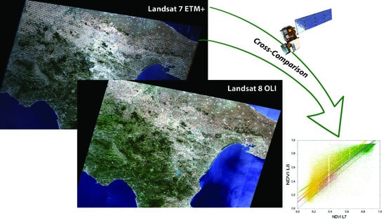
27], the cross-comparison between the Normalized Difference Vegetation Index (NDVI) extracted from Landsat 8 and Landsat 7 images, showed larger differences between NDVI calculated from the two generations of Landsat in lower vegetation covered areas; however, the difference decreases at higher vegetation cover (i.e., the NDVI values increase).
In other cases, even if the differences in terms of reflectance for the spectral bands [28] and other vegetation indices [29] was more significant, mainly for near infrared (NIR) and short wave infrared (SWIR), the regression analysis among the vegetation indices calculated with the two sensors provided high correlation values for other indices such as Land Surface Water Index (LSWI), NDVI and Normalized Burn Ratio (NBR) [28].
Within this context, vegetation indices are mostly implemented in the cross-comparison quantitative analysis [3,30,31,32,33] due to the low sensitivity to the atmospheric correction errors and to the different satellite visual angles. In particular, the NDVI is one of the most well-known and widely implemented at global scale for the environmental bio-physical characterization (vegetation cover, biomass, net primary production, etc.), climate changes, and environmental and hydrological modelling. A large set of intercalibration functions among NDVI indices from different sensors is reported in Steven et al. [7].
Among the various satellite platforms, Landsat can potentially provide long-term regional and global-scale high-quality NDVI data, thanks to the sensor’s high resolution. Indeed, NOAA (National Oceanic and Atmospheric Administration) Advanced Very High-Resolution Radiometer (AVHRR) has provided data since 1989 at 1 km geometric resolution, and since 1982 at 4 km geometric resolution. The SPOT (Satellite Pour l’Observation de la Terre) VEGETATION NDVI has provided NDVI data since 1999 at 1.5 km spatial resolution [34], while the Moderate Resolution Imaging Spectroradiometer (MODIS) NDVI datasets have been available since 2000 with different spatial resolutions, 250 m, 500 m, or 1 km [35].
The different Landsat generations, including the Landsat MSS, the Landsat 4-and 5 TM, the Landsat ETM+ and the current Landsat 8 Operational Land Imager (OLI), have provided data since 1972 [36], at 79 m spatial resolution before 1982, and at 30 m resolution since 1982.
In order to use long-term information, it is necessary to intercalibrate the images provided by the various Landsat sensor generations, obtaining standardized vegetation indices. Besides the NDVI, many other vegetation indices sensitive to the spectral bands difference effects (SBDE) have been formulated over the years, such as those resulting from the combination of visible bands as Atmospheric Resistant Vegetation Index (ARVI) and the Modified Triangular Vegetation Index (MTVI); whilst, the SBDE from other indices (e.g., Normalized Difference Water Index-NDWI, LSWI) have not been reported yet.
Landsat TM and ETM+ sensors allowed earth observation since the launch of Landsat 4 in 1982. The Landsat mission has continued with the Landsat 5 launched in 1984, carrying the same instrumentation of Landsat TM, and later with the launch of Landsat 7 in 1999 with the ETM+ sensor. The Landsat missions have provided a large amount of earth reflectance data collected in six spectral bands with different wavelengths at 30 m spatial resolution. Although the reflectance measured by TM and ETM+ sensors can be considered comparable, due to the similarities in the bandwidth and position, several studies on the intercalibration between the images yielded by different sensors have been carried out in order to provide long-term data [37]. The last Landsat generation satellite was launched on February 2013, initially known as the LDCM (Landsat Data Continuity Mission) was finally named Landsat-8. The satellite has been equipped with two new sensors: The Operational Land Imager (OLI), designed in order to operate in continuity with TM and ETM+; and the Thermal Infrared Sensor (TIRS), which features two bands in the thermal infrared region. The OLI sensor includes enhanced bands due to new linear detector arrays which collect images in a push-broom scanner mode providing a better signal with a high signal-to-noise ratio, compared to the previous whiskbroom scanner-based sensor [38]. The improved signal-to-noise performance is quantized over a 12-bit dynamic range, enabling a better land cover status characterization, with 12-bit images (scaled to 55,000 grey levels) [39]. Along these lines, the sensor is able to highlight a higher earth surface variability due to the maximization of the radiance ranges for all the spectral bands [40], and at the same time to reduce the saturation of highly reflective surfaces. However, the OLI sensor maintains the same geometric resolution, scene size (170 km × 183 km) and revisit time (16 days) compared to previous Landsat generations.
Thus, the main differences between OLI and previous TM and ETM+ sensors refer not only to the overall image quality but also to the different number of spectral bands, their width and their spatial resolutions [41]. In particular, the OLI sensor provides new bands such as: i) Band 1 (deep blue and violet) with a shorter wavelength (0.43–0.45 μm), also called the coastal/aerosol band due to its main uses; and ii) Band 9 covering a very short range of wavelengths in the short-wave infrared (1.36–1.39μm), also called Cirrus band due to its cloud cover sensing capacity (Table 1).
Furthermore, the Landsat 8 OLI bands are narrower compared to the Landsat 7 ETM+, avoiding atmospheric absorption [38]. In particular, the OLI NIR band is more similar to the MODIS NIR band, except for the 0.825 μm wavelength relative to the ETM+ for the absorption of water vapour [39]. The OLI Bands 6 and 7 are narrower compared to the ETM+ bands 5 and 7 respectively, reducing the atmospheric absorption and thus reducing the sensibility to atmospheric changes in terms of water vapour content.
To improve the standardization among different Landsat image generations, it is thus necessary to verify if the substantial differences between the two sensors regarding both bandwidth for the visible and SWIR, and the detection system technology, allowing for an efficient comparison among the images by the two sensors.
The main objectives of this study are: i) to extend the knowledge on the effects that the differences between Landsat 7 ETM+ and Landsat 8 OLI spectral responses may have through the analysis of different land use types through a wide range of derived vegetation indices; ii) to evaluate specific intercalibration functions for the standardization of vegetation indices in order to perform long-term time series analysis.
Up to date, the differences between Landsat 7 ETM+ and Landsat 8 OLI spectral responses have only been analyzed on a single derived vegetation index such as the NDVI, while in the present study, we extended the analysis to seven different indices and different land use types in order to achieve a more comprehensive analysis between the two sensors.

2. Materials and Methods

2.1. Study Area

The study area is located in the Basilicata region, in southern Italy (Figure 1). The Region can be considered representative for the Mediterranean area due to both climate and vegetation characteristics. In particular, the area is characterized by both a Mediterranean humid-type climate in the Apennine Mountains, and a Mediterranean dry-type climate in the hilly and flat areas. Forest vegetation covers 35.6% (355,367 ha) of the total area, represented by deciduous oak forests (51.8%), beech forests (8.4%), Mediterranean Macchia (7.9%), shrublands (6.9%), and other deciduous broad-leaved forests (5.5%) [42].
The analysis was performed in four rectangular plots covering an area of 4536 ha each, for a total area of 18,144 ha. The selected plot areas cover different land uses, climatic and orographic conditions. As shown in Table 1, the main land uses are “Forests” and “Arable lands” classes, representing 90% of the plot area. Other land uses are “Tree crops” (5%) and “Pastures and natural grasslands” (2%). Main differences in the plot areas depend on the distribution of the two main land use classes: i) plots 1 and 3 with predominant “Forests” class distribution; and ii) plots 2 and 4 with predominant “Arable lands” class distribution.

2.2. Spatial Data Preprocessing

To perform the cross-comparison analysis, the images from the two Landsat sensor generations have been selected according to the temporal proximity and to the overall quality, using the Global Visualization Viewer (Glovis) developed by the USGS Earth Resources Observation and Science Center (EROS). The selected scenes are the ETM+ SLC-off (Scan Line Corrector) (path = 188; row = 32), WRS2 (Worldwide Reference System2) (10/08/2017) and OLI (18/08/2017), classified as L1T (Level-1 Terrain-corrected) and registered to UTM coordinates, zone 33N, WGS84 Datum. The acquisition dates were chosen to minimize potential differences in terms of phenological phases between the ETM+ and OLI images.
Moreover, both Landsat ETM+ (26/08/2017) and MODIS (MOD09Q1, surface reflectance, band 1-2, 8-days composition) imageries have been downloaded and pre-processed in order to correct the NDVI variation caused by the 8-day time lag using the phenological patterns [27].
The land use information has been derived merging the Regional Agricultural Land Use Map, and the Regional Forest Map of Basilicata [42]. The land use classes in the two maps have been reclassified to reduce land use types (Table 2), as well as corrected through visual analysis based on the visual matching of land use classes from thematic maps compared to digital images form aerial orthophotos at 0.5 m spatial resolution TerraItaly 2008 data set.
According to several studies [43,44,45,46], both the radiometric calibration and the atmospheric correction represent a fundamental prerequisite for quantitative analyzes on Landsat data.
In particular, the radiometric calibration is required to convert the signal of quantified energy from digital numbers (DNs) into sensor radiance values, by using:
TOA = DN × G + B
where TOA (top-of-atmosphere) represent the radiance at the sensor for each band (W m−2 sr−1 μ−1); DN is the Digital Number value; G and B are respectively Gain and Bias values, calculated as follows:
B = Lmin − (LmaxLmin/QmaxQmin) × Qmin
G = (LmaxLmin/QmaxQmin)
where Lmin and Lmax represent minimum and maximum values of spectral radiance, as reported by the ETM+ and OLI image metadata files; Qmin and Qmax represent minimum and maximum values of DN for the two sensors, ranging from 1 to 255 for ETM+ and from 1 to 65,535 for OLI (16 bit images [47].
The atmospheric correction is necessary to reduce or normalize the modifications of the remotely sensed signal due to the intervening atmosphere between Earth’s surface and satellite. Although the atmospheric correction usually follows standardized procedures [48,49], it is a crucial pre-processing step, especially for data acquired by different sensors at different times, as well as to field-based and remote sensing data [49].
In this regard, we applied the 6SV atmospheric correction algorithm [50,51,52], which is one of the most effective methods for the atmospheric correction of different sensor spectral bands [7,53,54] and also for other applications [55,56,57,58,59,60].

2.3. Vegetation Indices

The ETM+ and OLI derived vegetation indices used for the cross-comparison analysis are reported in Table 3.
The NDVI is the first and most known vegetation index to explore and detect vegetated areas and plant canopies [61].
The NDWI, based on the combination of the green band with NIR or SWIR, is a good indicator for vegetation liquid water content and in the same time is less sensitive to atmospheric scattering effects than NDVI [62]. Its usefulness for drought monitoring and early warning has been demonstrated in different studies [63,64].
The LSWI (Land Surface Water Index) is sensitive to the total amount of liquid water in vegetation and in its soil background [62,65,66,67,68,69]. It is based on the SWIR1 and on the NIR regions of the electromagnetic spectrum. It is particularly used to detect the vegetation water content during the different phenological stages [70,71], and the inter-annual changes in vegetation water content related to climatic variations [66,72,73,74].
The NBR (Normalized Burn Ratio) index is used to detect the burnt areas and fire intensity [75,76,77,78,79]. The NIR band is sensitive to vegetation chlorophyll content, whilst the SWIR2 band is sensitive to soil and vegetation water content [80,81] providing information on typical conditions that occur after the fire events [82,83].
The EVI (Enhanced Vegetation Index) represents an improvement of NDVI, showing a reduced saturation in high vegetation cover regions, a reduction in atmospheric influences and a de-coupling of the canopy background signal [35,84,85]. These improvements are based on the introduction of the blue band to reduce the effects of the atmospheric aerosols in the red band, and on some correction coefficients to reduce the effect of soil reflectance. According to these differences, the NDVI is more sensitive to the chlorophyll content, whilst the EVI is more sensitive to the structural characteristics of the vegetation cover [86]. Thus, it has been widely used for Land Cover and Land Use/Land Cover Change detection [87], for the evaluation of vegetation bio-physical parameterization [88,89], phenology [85,90,91], evapotranspiration [73], biodiversity assessment [92], and gross primary production [93,94,95].
The SAVI (Soil-Adjusted Vegetation Index), proposed by Huete [96] reduces the effects of soil on vegetation reflectance [97,98].
The VIgreen (Vegetation Index Green) is sensitive to chlorophyll content and particularly to the photosynthetic active vegetation [99]. It has been used to detect the physiological conditions of the vegetation, the vegetation water content implemented in fuel models [100], the structural characteristics of the tree crops [101], and the phenology in agricultural crops [102].

2.4. Preliminary Analyzes

Due to the 8-day time lag between the Landsat ETM + and OLI image, a preliminary analysis was carried out on climatic data derived from the local meteorological stations in each considered plot. The occurrence of climatic events (especially with regard to precipitations) was verified, in order to remove any significant influence on the NDVI values, during the period between images. Over the 8-day time period (data processed from the Hydrological Annals from 10 to 18 August 2017) no anomalies were recorded that could significantly impact the NDVI values (Table 4).
However, in order to account for possible phenological effects that occurred over the 8-day time span, the vegetation growth rate was calculated using the MOD09Q1 MODIS product (surface reflectance 8 days composite):
r =     N D V I 26   a u g u s t N D V I 18   a u g u s t   N D V I 18   a u g u s t   N D V I 10   a u g u s t
Subsequently, to correlate the Landsat 8 NDVI of 18 August, the growth rate [5] between the 10 and 26 August ETM + images has been used:
N D V I E T M   18   a u g u s t =   N D V I E T M   26   a u g u s t   + r   N D V I E T M   10   a u g u s t 1 + r
where N D V I E T M   18   a u g u s t is the 18 August simulated Landsat ETM + NDVI, and N D V I E T M   26   a u g u s t   and N D V I E T M   10   a u g u s t are respectively the Landsat ETM + NDVI of 10 and 26 August.
The analysis carried out between the Landsat 8 OLI NDVI of August 18 and the simulated Landsat ETM + NDVI of August 18, and the Landsat ETM + of 10 August (Figure 2) also does not show significantly different values.
Thus, the comparison analysis between the two sensors has been performed for the all selected indices.

2.5. Statistical Analysis

According to the main studies on cross-comparison statistical analysis between different sensors [1,10,29,37,59,103], we performed for each test plot: i) the analysis of differences of the spectral responses between ETM+ and OLI for different land uses by estimating the differences between the reflectance average values of the two sensors and their dispersion. The analysis has been separately conducted for the main land uses in order to highlight potential spectral differences between them and the two sensors. ii) The analysis of differences in terms of descriptive statistic between different vegetation indices. In this ambit we analyzed the distribution of the different vegetation indices using indices of position and dispersion, highlighted through the box and whisker plots. Thus, the mean values and the measures of dispersion (mean + − SE and mean + − 2 SD) have been evaluated for the values of the indices differences and in order to examine the possible effects for different land use and environmental characteristics of each plot. The vegetation indices statistical significance difference has been also evaluated using the Student’s t-test, by considering the values of the indexes both on the whole image and on the stratified values, as a function of the land use. iii) the regression analysis between vegetation indices for the two sensors and for each plot, in order to evaluate a possible linear relationship between the two sensors, and consequently to assess the estimated intercalibration functions.

3. Results

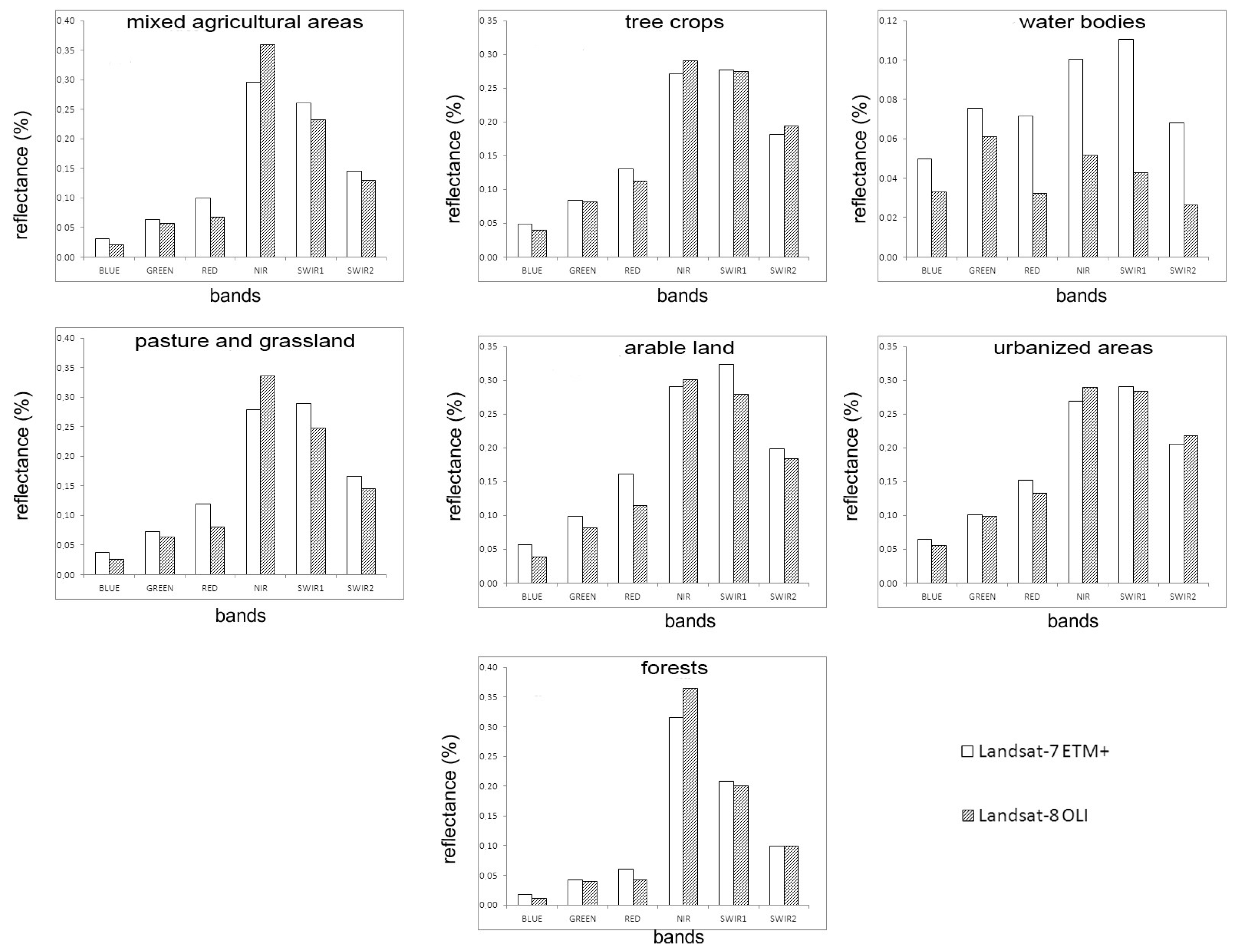
Figure 3 shows significant differences in the average reflectance values between the ETM+ and OLI bands by land use classes. In particular, the OLI NIR band seems to be more sensitive (higher average reflectance value compared to ETM+) in the forest class, while the reflectance in the visible band (and especially in the red one) is greater in ETM+ than OLI, determining the higher values of OLI NDVI than ETM+ NDVI.
The SWIR1 and SWIR2 infrared bands show few differences for the forest land use class with a slight absorption for the SWIR1 OLI band. The NIR OLI band shows higher average reflectance value than ETM+ for the land use classes characterized by high vegetation cover than for low vegetation cover areas (arable lands, urbanized areas). The SWIR (SWIR1 e SWIR2) OLI bands show higher absorption values than ETM+, although these differences tend to decrease in the area with high vegetation cover. The highest differences between the two sensors refer to the water bodies with significantly higher average reflectance values for all the ETM+ bands, and particularly for the SWIR1 band. The sensor sensitivity to visible bands shows an opposite behaviour for the NIR, in all the land use classes, with ETM+ average reflectance values constantly higher than OLI (especially for the red band) with significant differences for pastures, arable lands, and water bodies. To compare the ETM+ and OLI derived vegetation indices, for the 4 plots, the NDVI, LSWI, NDWI, NBR, VIgreen, SAVI, and EVI have been calculated from the ETM+ and OLI images. The Student’s t-test results (Table 5) show a significant difference between the ETM+ and OLI derived vegetation indices (NDVI, LSWI, NDWI, NBR, VIgreen, SAVI, and EVI) for the 4 plots.
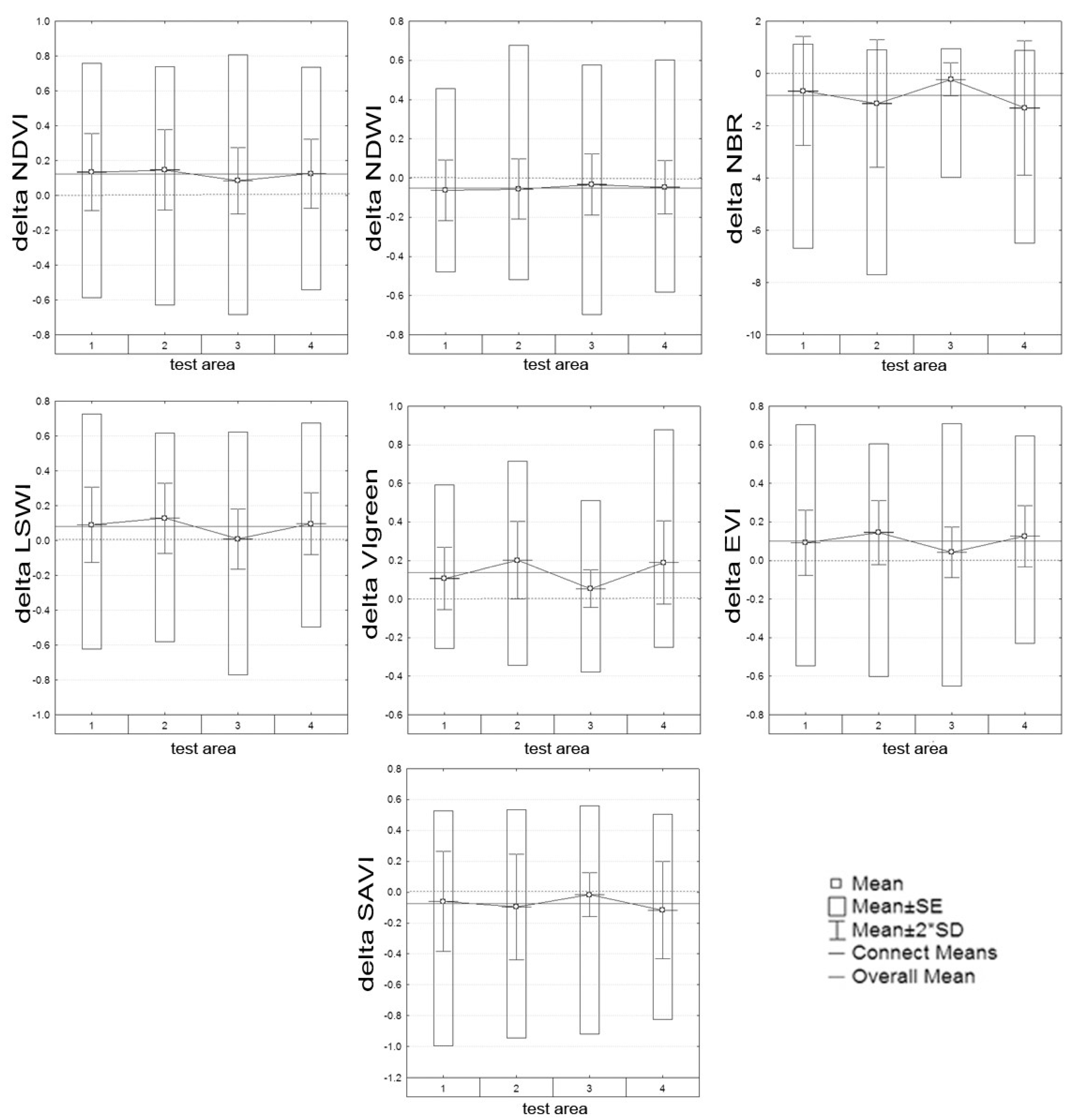
As shown in Figure 4, there are relevant dissimilarities between the two sensors in all indices. The NDWI, SAVI, and LSWI indices show the higher correlation between the two sensors with a mean difference of −0.0500, −0.0725, and 0.0819, respectively. Instead, the standard deviation is smaller than the other indices. The other indices (NDVI, VIgreen, and EVI), with the exception of NBR (which has the difference average value equal to −0.8446, and the standard deviation of 1.27) show difference average values higher than 0.1. Among these, the EVI shows a greater similarity between the two sensors (with very low deviations), followed by the NDVI with an average difference value equal to 0.1223. The VIgreen shows the higher differences between OLI and ETM+ (average difference value equal to 0.1367).
The indices based on non-visible bands combinations (LSWI and NBR) are therefore sufficiently similar and stable between the two sensors, with few fluctuations in the average difference over the four plots. However, the NDVI and NDWI show the greater stability in the different plots with very few fluctuations. The NDWI also shows the lower differences between the two sensors in all the plots. The VIgreen index shows the lower stability, confirming that indices using only visible bands show higher variation due to the SBDE (spectral difference between bands) [2,29].
In particular, these results are related to the main differences in the red band between the two sensors for all the land uses with the exception of urbanized areas. Figure 4 was characterized by small differences in every index. This can be attributed to the morphological characteristics of the area depending on climatic conditions and on land use classes. In particular the plot 4 (Table 2), located in the Southeast of the regional survey area, is characterized by low altitude and flat terrain. As for the land use classes, Figure 4 shows a predominance of arable land (about 50% of the area), followed by forests, for about 1/3 of the entire area, and tree crops that reach here the greater extension (12% of the plot area) among all the plots.
The results of the analysis of the difference variability between the vegetation indices for each of the test area and for each land use class are reported in Figure 5 and Table 6.
The results in Table 6 show that, for almost all the considered indices, statistically significant differences exist between the two sensors by land use class. Only for water bodies class, NDWI (often used for the identification of wet areas), SAVI and EVI indices do not show significant differences between the sensors, and SAVI also does not show significant differences for the Urbanized and Mixed agricultural areas classes. This result also confirms the robustness of the correction of the soil brightness introduced in the index for both sensors, for the discrimination of the classes in which the vegetation is absent (Urbanized areas) or it is interspersed with bare soils (Mixed agricultural areas).
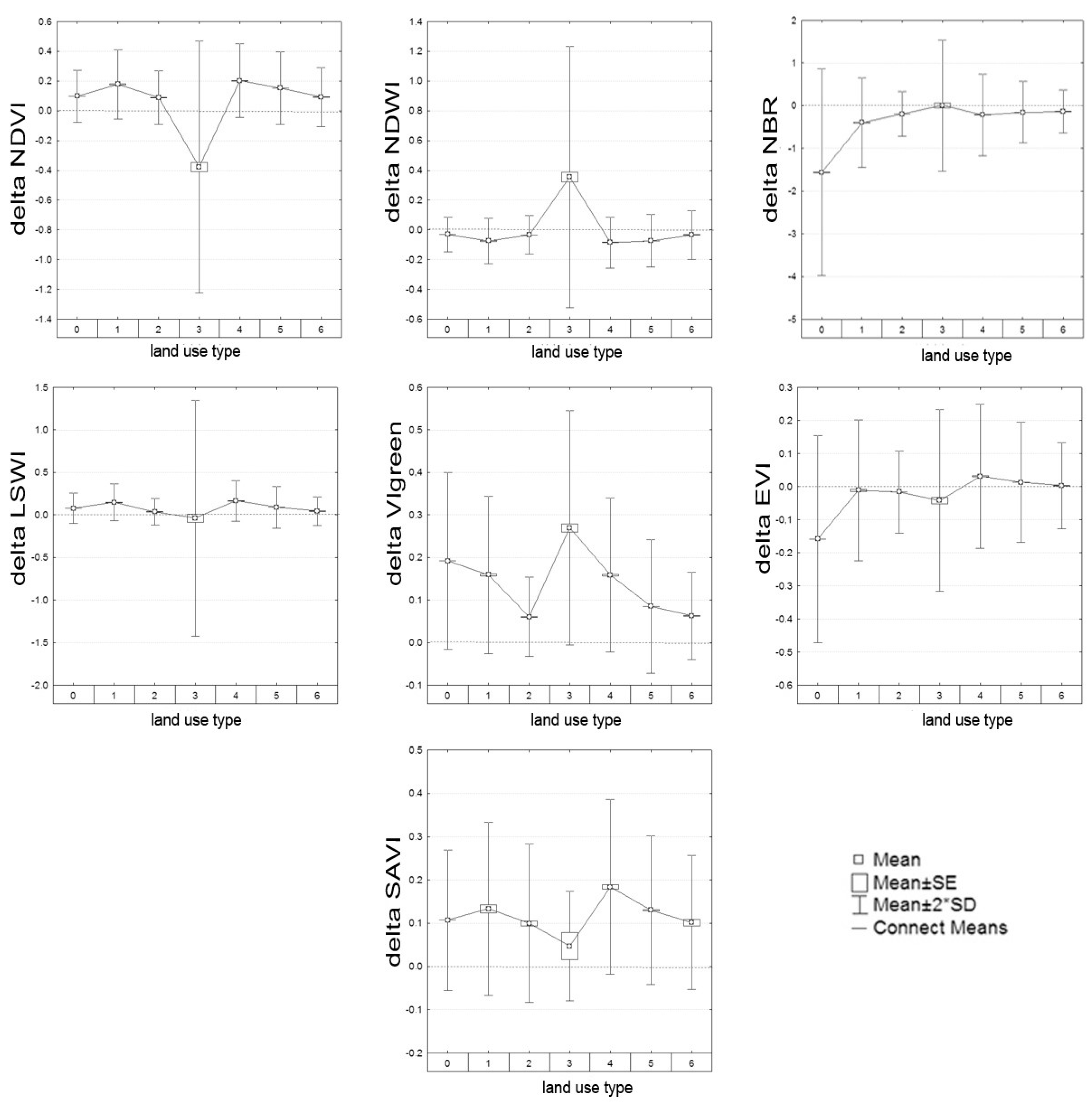
According to the box-plot results showed in Figure 5, for forest land use, some indices based on the combination of NIR and Red (SAVI and EVI) show a remarkable difference between the two sensors with significant variability. The same performance for the forest land use has been found in NBR, based on the combination of infrared bands, and VIgreen, based only on visible bands. NDVI and NDWI for forest land use show good results with low average difference values and low variability. Tree crops show average difference values generally close to zero and low variability with respect to the other land uses for all indices.
Even arable land classes show a similar trend to the tree crops with generally low average difference values between the two sensors, both for the vegetation indices based on the combination of infrared bands (NBR, LSWI), and based only on visible bands (VIgreen).
The plot 4, characterized by a lower percentage of forest land use cover and combined with the higher percentage of tree crops cover and high arable lands cover, shows a low variability of the average difference values for all the vegetation indices.
Plots 1 and 2, characterized by a higher percentage of forest land use cover (more than 60% of the plot area), by a lower percentage cover of arable land, and by a significant reduction, compared to the fourth plot, of tree crops land use (respectively 0.1% and 2% of the surface of the plot), show the highest variability for all vegetation indices.
Finally, the regression analysis between the vegetation indices ETM+ based and OLI based has been conducted in order to identify the intercalibration functions between the two sensors datasets. The goodness of fit of the OLS regressions were defined by the coefficient of determination (R2) and the significance of the OLS regressions was defined by examination of the regression overall F-statistic p-value. To provide simple overall measures of similarity, the Root Mean Square Deviation between the OLI and ETM+ data has derived:
R M S D =   i n ( v i O L I v i E T M + ) 2 n
The identified functions and the related indices (Table 7) show a good linear relationship between the dependent variables (indices calculated with OLI) and the independent variables (indices calculated with ETM+). The intercalibration functions, however, show significant dissimilarities among vegetation indices: the indices based on the combination between infrared and visible bands (NDVI, NDWI, SAVI, and EVI) show a better correlation with a determination coefficient always higher than 0.8. Instead, the indices based only on infrared (NBR and LSWI) or on visible bands (VIgreen) show a lower correlation. In particular, the VIgreen shows a determination coefficient less than 0.5, highlighting the differences SBDE in the range of the visible waveband, and, thus, confirming the previously described analysis.
NBR and LSWI also show a poor correlation, particularly for NBR, which highlight the existence of a non-linear component between the two sensors. In addition, in this case, the differences are most likely related to SBDE, as for the bands SWIR highlighting a significant difference in the bandwidth between the two sensors.
From the regression analysis, it has been found that lowest values are reported in plot 4, whilst plot 2 and 3 show higher correlation values. In particular, plot 4 is characterized by the lowest average values for all the calculated vegetation indices, whilst plot 2 and 3 are characterized by highest average values for all the calculated vegetation indices.
These differences also suggest that the higher variability within vegetation indices values occur within areas characterized by low vegetation indices values and thus for areas with a low percentage of vegetation cover. 
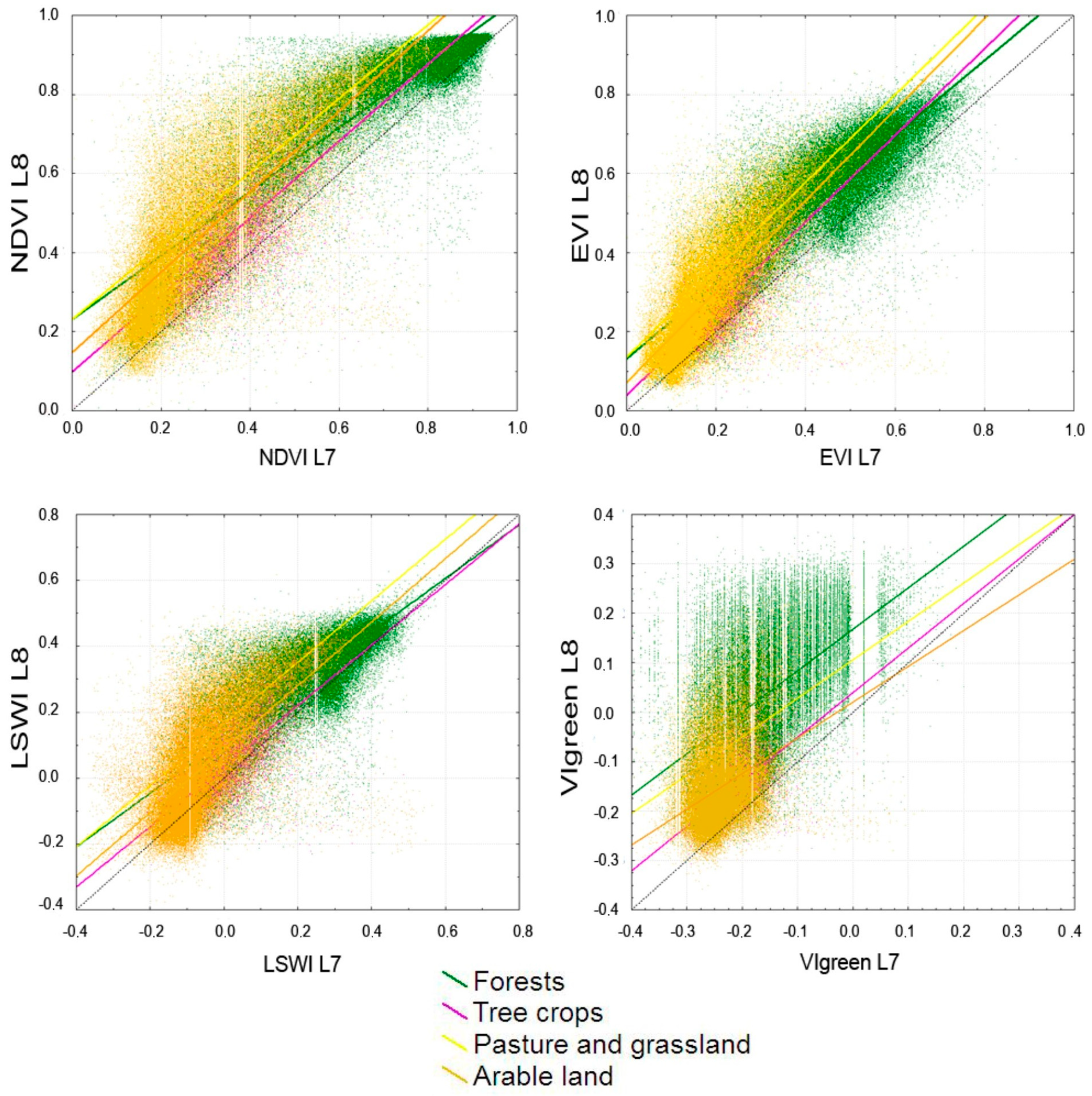
Figure 6 shows different trends according to the land use type and vegetation index. The OLI NDVI is always higher than the ETM+ NDVI in all land uses, with higher differences for pasture and arable land and a decrease for tree crops and forests. This may suggest that the greatest differences of index values are related to low biomass content (pastures and arable land), whilst lower differences are related to the high value of biomass content. In particular, pasture, arable lands and tree crops show a regression function with a slope almost parallel to the 1:1 line, and forest land use shows the largest differences for lower NDVI values. With the increase of the index value, there is a constant reduction of the differences between OLI and ETM+ derived indices. The EVI shows the same trends described for NDVI and for indices based on the normalized difference of infrared bands (LSWI in Figure 6). VIgreen, based on visible bands (green and red), shows the greatest differences for land use classes characterized by high values of vegetation cover (forests) with differences nearly constant. This confirms the existence of differences due to SBDE between the two sensors in the visible range, especially with respect to the red band. For arable land, the trends of the index are different because OLI is higher than ETM+. For low index values, the increase of the VIgreen values ETM+ is higher than OLI ones due to a greater absorption in OLI red band together with the intensification of the vegetation cover.

4. Discussions

The comparison between Landsat 7 ETM+ and Landsat 8 OLI to identify the main differences between the two sensors and the spectral responses for different land uses presented in this study, showed significant differences among spectral ranges and vegetation indices derived from the two sensors. However, the 8-day difference between the two Landsat 7 ETM+ and Landsat 8 OLI scenes and the period of the analysis minimizes the effects of vegetation phenology and thus increasing the reliability of the results of the present study. The comparison among the spectral bands provided by the two sensors showed a good similarity. Nevertheless, significant differences are evident in the various spectral ranges: i) high reflectance values of OLI in the band of NIR for all the land use classes, particularly for high values of vegetation cover, ii) and lower reflectance in the SWIR bands, especially for low vegetation cover land uses as for the pastures and grasslands. There are decreasing differences in SWIR band with the increase of biomass values up to maximum values represented by forest cover.
For the visible bands, the ETM+ sensor shows reflectance values greater than OLI ones. The analysis of vegetation indices based on the two sensors shows low differences between the indices based on the combination of NIR and visible bands (NDVI, EVI, NDWI, and SAVI), whilst the indices based only on the visible bands (VIgreen) or only on the infrared bands such as NBR, show higher values of difference. A different result is showed by the analysis of LSWI which, according to the results showed by Li et al. [29], is not only more similar but also more stable between the two sensors, with low fluctuations in the various plot areas. The regression analysis among the vegetation indices calculated with the two sensors highlights a good correlation, especially for NDVI, NDWI, SAVI, and EVI, with an index of determination higher than 0.8. On the other hand, both VIgreen and NBR show a high dispersion, probably due to the differences in the spectral response of corresponding bands.
With regard to the study of the intercalibration functions between ETM+ and OLI derived vegetation indices for the Mediterranean region is fundamental to ensure an effective operational continuity between the current and previous Landsat missions.
As showed by the literature and confirmed by the results of this study, the two sensors derived vegetation indices are not directly comparable. Differences between Landsat 7 ETM+ and Landsat 8 OLI vegetation indices are directly related to the different width of spectral bands and to the different radiometric resolution between the two sensors [104].
Different studies showed how the differences for high values of NDVI are directly related to the spectral bandwidth; other studies highlighted the inverse relationship between the increases in bandwidth and mean NDVI values [46].
Another factor affecting the differences of vegetation indices between the two sensors, and in particular, the dynamic range of vegetation indices, is the difference in spectral band resolution [105]: the higher is the number of bits, the higher is the variability of the estimated index. According to this, the Landsat 8 OLI derived vegetation indices represent an effective tool to study the ecosystem variability in the Mediterranean region, characterized by a very high land use and land cover variability, due to the combination of both land management practices and physical characteristics mainly related to high climatic variability.

5. Conclusions

Landsat satellite systems represent a fundamental tool for the study of long-term environmental and land use/land cover dynamics at a global scale. The long-term dataset availability combined with the increased processing capacity, contributed to an increase of the number of studies, observation programs and land cover monitoring tasks. In order to emphasize and standardize the available dataset provided by different missions and to allow reliable and site specific multi-temporal analysis, it is important to define intercalibration algorithms between the different missions. The high ecosystem spatial and temporal variability, characterizing the Mediterranean region, represents a real challenge to develop reliable intercalibration algorithms between the two sensors. The results of this study showed an overall good correlation between indices calculated with the two sensors; while according to single land use classes, statistically significant differences was found for almost all the indices analyzed. According to these observations, a greater attention needs to be addressed in long-term environmental and land use/land cover dynamics analysis in the Mediterranean region. In particular, the very fast land use/land cover changes characterizing this region under the ongoing climate change scenario, are mainly due to the combination of both natural and anthropogenic drivers. Such variability combined with sensor’s differences may lead to wrong estimates and thus wrong interpretation of environmental patterns of main vegetation indices. In particular, more attention needs to be addressed to differences between the two sensors in the evaluation of infrared (NIR and SWIR) based indices for the estimation of both vegetation and soil water content, which represent highly climate sensitive key indicators in the Mediterranean environment.

Author Contributions

Conceptualization, G.M.; Methodology, G.M. and A.N.; Software, G.M. and A.N.; Validation, G.M.; Formal Analysis, G.M.; Investigation, G.M. and A.N.; Resources, G.M. and A.F.; Data Curation, G.M.; Writing-Original Draft Preparation, G.M., A.F. and A.N.; Writing-Review & Editing, G.M., A.F., A.P. and A.N.; Visualization, G.M., A.F. and A.N.; Supervision, G.M.; Project Administration, A.F.; Funding Acquisition, A.F. All authors have read and agreed to the published version of the manuscript.

Funding

This research received no external funding.

Acknowledgments

This research was supported by Italian MIUR Project (MIUR-PRIN 2010-2011) “Climate change mitigation strategies in tree crops and forestry in Italy (CARBOTREES)” (P.I. Agostino Ferrara).

Conflicts of Interest

The authors declare no conflict of interest. The founding sponsors had no role in the design of the study; in the collection, analyses, or interpretation of data; in the writing of the manuscript, and in the decision to publish the results.

References

  1. Anderson, J.H.; Weber, K.T.; Gokhale, B.; Chen, F. Intercalibration and Evaluation of ResourceSat-1 and Landsat-5 NDVI. Can. J. Remote Sens. 2011, 37, 213–219. [Google Scholar] [CrossRef]
  2. Teillet, P.M.; Ren, X. Spectral band difference effects on vegetation indices derived from multiple satellite sensor data. Can. J. Remote Sens. 2008, 34, 159–173. [Google Scholar]
  3. Gallo, K.; Ji, L.; Reed, B.; Eidenshink, J.; Dwyer, J. Multi-platform comparisons of MODIS and AVHRR normalized difference vegetation index data. Remote Sens. Environ. 2005, 99, 221–231. [Google Scholar] [CrossRef] [Green Version]
  4. Huete, A.; Yoshioka, H.; Miura, T.; Kim, H.J.; Gao, X. Inter-sensor calibration of vegetation indices for monitoring and continuity studies of ecosystem variability. In First International Symposium on Recent Advances in Quantitative Remote Sensing; Sobrino, J.A., Ed.; Universitat de València: València, Spain, 2002. [Google Scholar]
  5. Thome, K.J.; Barnes, R.A.; Feldman, G. Intercomparison of ETM+, MODIS, and SeaWiFS using a land test site. In Proceedings of the Sensors, Systems, and Next-Generation Satellites VI International Society for Optics and Photonics, Crete, Greece, 8 April 2003. [Google Scholar] [CrossRef]
  6. Rao, C.R.N.; Cao, C.; Zhang, N. Inter-calibration of the Moderate-Resolution Imaging Spectroradiometer and the AlongTrack Scanning Radiometer-2. Int. J. Remote Sens. 2003, 24, 1913–1924. [Google Scholar] [CrossRef]
  7. Steven, M.D.; Malthus, T.J.; Baret, F.; Xu, H.; Chopping, M.J. Intercalibration of vegetation indices from different sensor systems. Remote Sens. Environ. 2003, 88, 412–422. [Google Scholar] [CrossRef]
  8. Teillet, P.M.; Fedosejevs, G.; Gauthier, R.P.; O’Neill, N.T.; Thome, K.J.; Biggar, S.F.; Ripley, H.; Meygret, A. A generalized approach to the vicarious calibration of multiple Earth observation sensors using hyperspectral data. Remote Sens. Environ. 2001, 77, 304–327. [Google Scholar] [CrossRef]
  9. Teillet, P.M.; Fedosejevs, G.; Thome, K.J. Spectral band difference effects on radiometric cross-calibration between multiple satellite sensors in the Landsat solar-reflective spectral domain. In Proceedings of the Sensors, Systems, and Next-Generation Satellites VIII, Maspalomas, Canary Islands, Spain, 4 November 2004; p. 10. [Google Scholar]
  10. Chen, X.; Vogelmann, J.E.; Chander, G.; Ji, L.; Tolk, B.; Huang, C.; Rollins, M. Cross-sensor comparisons between Landsat 5 TM and IRS-P6 AWiFS and disturbance detection using integrated Landsat and AWiFS time-series images. Int. J. Remote Sens. 2013, 34, 2432–2453. [Google Scholar] [CrossRef]
  11. Guyot, G.; Gu, X.-F. Effect of radiometric corrections on NDVI-determined from SPOT-HRV and Landsat-TM data. Remote Sens. Environ. 1994, 49, 169–180. [Google Scholar] [CrossRef]
  12. Hill, J.; Aifadopoulou, D. Comparative analysis of landsat-5 TM and SPOT HRV-1 data for use in multiple sensor approaches. Remote Sens. Environ. 1990, 34, 55–70. [Google Scholar] [CrossRef]
  13. Martinez Beltran, C.; Calera, A.; Jochum, A. Inter-satellite cross-calibration: Integration of reflectance and NDVI from different satellites by means of a linear model. In Proceedings of the Remote Sensing for Agriculture, Ecosystems, and Hydrology V. International Society for Optics and Photonics, Barcelona, Spain, 24 February 2004. [Google Scholar] [CrossRef]
  14. Oguro, Y.; Tsuchiya, K.; Suga, Y. Comparison of land cover features observed with different satellite sensors over a semi-arid land in central Australia. Adv. Space Res. 1999, 23, 1401–1404. [Google Scholar] [CrossRef]
  15. Oguro, Y.; Suga, Y.; Takeuchi, S.; Ogawa, M.; Konishi, T.; Tsuchiya, K. Comparison of SAR and optical sensor data for monitoring of rice plant around Hiroshima. Adv. Space Res. 2001, 28, 195–200. [Google Scholar] [CrossRef]
  16. Thome, K.J.; Biggar, S.F.; Wisniewski, W. Cross comparison of EO-1 sensors and other Earth resources sensors to Landsat-7 ETM+ using Railroad Valley Playa. IEEE Trans. Geosci. Remote Sens. 2003, 41, 1180–1188. [Google Scholar] [CrossRef] [Green Version]
  17. Van Wagtendonk, J.W.; Root, R.R.; Key, C.H. Comparison of AVIRIS and Landsat ETM+ detection capabilities for burn severity. Remote Sens. Environ. 2004, 92, 397–408. [Google Scholar] [CrossRef]
  18. Vázquez, A.; Cuevas, J.M.; González-Alonso, F. Comparison of the use of WiFS and LISS images to estimate the area burned in a large forest fire. Int. J. Remote Sens. 2001, 22, 901–907. [Google Scholar] [CrossRef]
  19. Gallo, K.P.; Daughtry, C.S.T. Differences in vegetation indices for simulated Landsat-5 MSS and TM, NOAA-9 AVHRR, and SPOT-1 sensor systems. Remote Sens. Environ. 1987, 23, 439–452. [Google Scholar] [CrossRef]
  20. Gong, P.; Wang, J.; Yu, L.; Zhao, Y.; Zhao, Y.; Liang, L.; Niu, Z.; Huang, X.; Fu, H.; Liu, S.; et al. Finer resolution observation and monitoring of global land cover: First mapping results with Landsat TM and ETM+ data. Int. J. Remote Sens. 2013, 34, 2607–2654. [Google Scholar] [CrossRef] [Green Version]
  21. Oguro, Y.; Suga, Y.; Takeuchi, S.; Ogawa, H.; Tsuchiya, K. Monitoring of a rice field using landsat-5 TM and landsat-7 ETM+ data. Adv. Space Res. 2003, 32, 2223–2228. [Google Scholar] [CrossRef]
  22. Röder, A.; Kuemmerle, T.; Hill, J. Extension of retrospective datasets using multiple sensors. An approach to radiometric intercalibration of Landsat TM and MSS data. Remote Sens. Environ. 2005, 95, 195–210. [Google Scholar] [CrossRef]
  23. Serra, P.; Pons, X.; Saurí, D. Post-classification change detection with data from different sensors: Some accuracy considerations. Int. J. Remote Sens. 2003, 24, 3311–3340. [Google Scholar] [CrossRef]
  24. Teillet, P.M.; Barker, J.L.; Markham, B.L.; Irish, R.R.; Fedosejevs, G.; Storey, J.C. Radiometric cross-calibration of the Landsat-7 ETM+ and Landsat-5 TM sensors based on tandem data sets. Remote Sens. Environ. 2001, 78, 39–54. [Google Scholar] [CrossRef] [Green Version]
  25. Teillet, P.M.; Markham, B.L.; Irish, R.R. Landsat cross-calibration based on near simultaneous imaging of common ground targets. Remote Sens. Environ. 2006, 102, 264–270. [Google Scholar] [CrossRef] [Green Version]
  26. Teillet, P.M.; Fedosejevs, G.; Thome, K.J.; Barker, J.L. Impacts of spectral band difference effects on radiometric cross-calibration between satellite sensors in the solar-reflective spectral domain. Remote Sens. Environ. 2007, 110, 393–409. [Google Scholar] [CrossRef]
  27. Xu, D.; Guo, X. Compare NDVI Extracted from Landsat 8 Imagery with that from Landsat 7 Imagery. Am. J. Remote Sens. 2014, 2, 10–14. [Google Scholar] [CrossRef] [Green Version]
  28. Mishra, N.; Obaidul Haque, M.; Leigh, L.; Aaron, D.; Helder, D.; Markham, B. Radiometric Cross Calibration of Landsat 8 Operational Land Imager (OLI) and Landsat 7 Enhanced Thematic Mapper Plus (ETM+). Remote Sens. 2014, 6, 12619–12638. [Google Scholar] [CrossRef] [Green Version]
  29. Li, P.; Jiang, L.; Feng, Z. Cross-Comparison of Vegetation Indices Derived from Landsat-7 Enhanced Thematic Mapper Plus (ETM+) and Landsat-8 Operational Land Imager (OLI) Sensors. Remote Sens. 2014, 6, 310–329. [Google Scholar] [CrossRef] [Green Version]
  30. Fensholt, R.; Sandholt, I.; Stisen, S. Evaluating MODIS, MERIS, and VEGETATION vegetation indices using in situ measurements in a semiarid environment. IEEE Trans. Geosci. Remote Sens. 2006, 44, 1774–1786. [Google Scholar] [CrossRef]
  31. Gitelson, A.A.; Kaufman, Y.J. MODIS NDVI Optimization to Fit the AVHRR Data Series—Spectral Considerations. Remote Sens. Environ. 1998, 66, 343–350. [Google Scholar] [CrossRef]
  32. Trenberth, K.E.; Anthes, R.A.; Belward, A.; Brown, O.; Habermann, T.; Karl, T.R.; Running, S.; Trishchenko, A.P.; Cihlar, J.; Li, Z. Effects of Spectral Response Function on Surface Reflectance and NDVI Measured with Moderate Resolution Satellite Sensors. Remote Sens. Environ. 2002, 811, 811–818. [Google Scholar]
  33. Van Leeuwen, W.J.D.; Orr, B.J.; Marsh, S.E.; Herrmann, S.M. Multi-sensor NDVI data continuity: Uncertainties and implications for vegetation monitoring applications. Remote Sens. Environ. 2006, 100, 67–81. [Google Scholar] [CrossRef]
  34. Barichivich, J.; Briffa, K.R.; Myneni, R.B.; Osborn, T.J.; Melvin, T.M.; Ciais, P.; Piao, S.; Tucker, C. Large-scale variations in the vegetation growing season and annual cycle of atmospheric CO2 at high northern latitudes from 1950 to 2011. Glob. Chang. Biol. 2013, 19, 3167–3183. [Google Scholar] [CrossRef]
  35. Huete, A.; Didan, K.; Miura, T.; Rodriguez, E.P.; Gao, X.; Ferreira, L.G. Overview of the radiometric and biophysical performance of the MODIS vegetation indices. Remote Sens. Environ. 2002, 83, 195–213. [Google Scholar] [CrossRef]
  36. Kovalskyy, V.; Roy, D.P. The global availability of Landsat 5 TM and Landsat 7 ETM+ land surface observations and implications for global 30m Landsat data product generation. Remote Sens. Environ. 2013, 130, 280–293. [Google Scholar] [CrossRef] [Green Version]
  37. Chander, G.; Hewison, T.J.; Fox, N.; Wu, X.; Xiong, X.; Blackwell, W.J. Overview of Intercalibration of Satellite Instruments. IEEE Trans. Geosci. Remote Sens. 2013, 51, 1056–1080. [Google Scholar] [CrossRef]
  38. Irons, J.R.; Dwyer, J.L.; Barsi, J.A. The next Landsat satellite: The Landsat Data Continuity Mission. Remote Sens. Environ. 2012, 122, 11–21. [Google Scholar] [CrossRef] [Green Version]
  39. Roy, D.P.; Wulder, M.A.; Loveland, T.R.; Woodcock, C.E.; Allen, R.G.; Anderson, M.C.; Helder, D.; Irons, J.R.; Johnson, D.M.; Kennedy, R.; et al. Landsat-8: Science and product vision for terrestrial global change research. Remote Sens. Environ. 2014, 145, 154–172. [Google Scholar] [CrossRef] [Green Version]
  40. Markham, B.L.; Helder, D.L. Forty-year calibrated record of earth-reflected radiance from Landsat: A review. Remote Sens. Environ. 2012, 122, 30–40. [Google Scholar] [CrossRef] [Green Version]
  41. United States Geological Survey-USGS. Available online: https://www.usgs.gov/land-resources/nli/landsat (accessed on 1 July 2019).
  42. Costantini, G.; Bellotti, A.; Mancino, G.; Borghetti, M.; Ferrara, A. Carta forestale della Basilicata—Atlante. INEA Reg. Basilicata Potenza 2006, 3, 325–326. [Google Scholar]
  43. Gordon, H.R. Calibration requirements and methodology for remote sensors viewing the ocean in the visible. Remote Sens. Environ. 1987, 22, 103–126. [Google Scholar] [CrossRef]
  44. Mancino, G.; Nole, A.; Urbano, V.; Amato, M.; Ferrara, A. Assessing water quality by remote sensing in small lakes: The case study of Monticchio lakes in southern Italy. iForest Biogeosci. For. 2009, 2, 154. [Google Scholar] [CrossRef] [Green Version]
  45. Mancino, G.; Nole, A.; Ripullone, F.; Ferrara, A. Landsat TM imagery and NDVI differencing to detect vegetation change: Assessing natural forest expansion in Basilicata, southern Italy. iForest Biogeosci. For. 2014, 7, 76–85. [Google Scholar] [CrossRef] [Green Version]
  46. Teillet, P.M.; Staenz, K.; William, D.J. Effects of spectral, spatial, and radiometric characteristics on remote sensing vegetation indices of forested regions. Remote Sens. Environ. 1997, 61, 139–149. [Google Scholar] [CrossRef]
  47. Landsat.Usgs.Gov. Landsat 8 (L8) Data Users Handbook, Version 5.0. Available online: Http://Landsat.Usgs.Gov (accessed on 6 June 2018).
  48. Schroeder, T.A.; Cohen, W.B.; Song, C.; Canty, M.J.; Yang, Z. Radiometric correction of multi-temporal Landsat data for characterization of early successional forest patterns in western Oregon. Remote Sens. Environ. 2006, 103, 16–26. [Google Scholar] [CrossRef]
  49. Young, N.E.; Anderson, R.S.; Chignell, S.M.; Vorster, A.G.; Lawrence, R.; Evangelista, P.H. A survival guide to Landsat preprocessing. Ecology 2017, 98, 920–932. [Google Scholar] [CrossRef] [PubMed] [Green Version]
  50. Vermote, E.F.; Tanre, D.; Deuze, J.L.; Herman, M.; Morcette, J. Second Simulation of the Satellite Signal in the Solar Spectrum, 6S: An overview. IEEE Trans. Geosci. Remote Sens. 1997, 35, 675–686. [Google Scholar] [CrossRef] [Green Version]
  51. Ouaidrari, H.; Vermote, E.F. Operational Atmospheric Correction of Landsat TM Data. Remote Sens. Environ. 1999, 70, 4–15. [Google Scholar] [CrossRef]
  52. Kotchenova, S.Y.; Vermote, E.F.; Matarrese, R.; Klemm, J.F.J. Validation of a vector version of the 6S radiative transfer code for atmospheric correction of satellite data. Part I: Path radiance. Appl. Opt. 2006, 45, 6762–6774. [Google Scholar] [CrossRef] [Green Version]
  53. Vermote, E.F.; Vermeulen, A. Atmospheric correction algorithm: Spectral reflectances (MOD09). ATBD Version 1999, 4, 1–107. [Google Scholar]
  54. Kotchenova, S.Y.; Vermote, E.F.; Levy, R.; Lyapustin, A. Radiative transfer codes for atmospheric correction and aerosol retrieval: Intercomparison study. Appl. Opt. 2008, 47, 2215–2226. [Google Scholar] [CrossRef] [Green Version]
  55. Alencar, A.; Asner, G.P.; Knapp, D.; Zarin, D. Temporal variability of forest fires in eastern Amazonia. Ecol. Appl. 2011, 21, 2397–2412. [Google Scholar] [CrossRef]
  56. Fensholt, R.; Sandholt, I.; Stisen, S.; Tucker, C. Analysing NDVI for the African continent using the geostationary meteosat second generation SEVIRI sensor. Remote Sens. Environ. 2006, 101, 212–229. [Google Scholar] [CrossRef]
  57. Vermote, E.; Ellicott, E.; Dubovik, O.; Lapyonok, T.; Chin, M.; Giglio, L.; Roberts, G.J. An approach to estimate global biomass burning emissions of organic and black carbon from MODIS fire radiative power. J. Geophys. Res. Atmos. 2009, 114, D18205. [Google Scholar] [CrossRef]
  58. Hansen, M.C.; Loveland, T.R. A review of large area monitoring of land cover change using Landsat data. Remote Sens. Environ. 2012, 122, 66–74. [Google Scholar] [CrossRef]
  59. Flood, N. Continuity of Reflectance Data between Landsat-7 ETM+ and Landsat-8 OLI, for Both Top-of-Atmosphere and Surface Reflectance: A Study in the Australian Landscape. Remote Sens. 2014, 6, 7952–7970. [Google Scholar] [CrossRef] [Green Version]
  60. Roy, D.P.; Kovalskyy, V.; Zhang, H.K.; Vermote, E.F.; Yan, L.; Kumar, S.S.; Egorov, A. Characterization of Landsat-7 to Landsat-8 reflective wavelength and normalized difference vegetation index continuity. Remote Sens. Environ. 2016, 185, 57–70. [Google Scholar] [CrossRef] [Green Version]
  61. Rouse, J.W.; Haas, R.H.; Schell, J.A.; Deering, D.W. Monitoring vegetation systems in the Great Plains with ERTS. In Proceedings of the 3rd ERTS Symposium, Washington, DC, USA, 10–14 December 1973; NASA-SP-351-Vol-1-Sect-A. Volume 1, pp. 309–317. [Google Scholar]
  62. Gao, B.-C. NDWI—A normalized difference water index for remote sensing of vegetation liquid water from space. Remote Sens. Environ. 1996, 58, 257–266. [Google Scholar] [CrossRef]
  63. Gu, Y.; Brown, J.F.; Verdin, J.P.; Wardlow, B. A five-year analysis of MODIS NDVI and NDWI for grassland drought assessment over the central Great Plains of the United States. Geophys. Res. Lett. 2007, 34, L06407. [Google Scholar] [CrossRef] [Green Version]
  64. Ceccato, P.; Flasse, S.; Grégoire, J.-M. Designing a spectral index to estimate vegetation water content from remote sensing data: Part 2. Validation and applications. Remote Sens. Environ. 2002, 82, 198–207. [Google Scholar] [CrossRef]
  65. Boles, S.H.; Xiao, X.; Liu, J.; Zhang, Q.; Munkhtuya, S.; Chen, S.; Ojima, D. Land cover characterization of Temperate East Asia using multi-temporal VEGETATION sensor data. Remote Sens. Environ. 2004, 90, 477–489. [Google Scholar] [CrossRef]
  66. Fensholt, R.; Sandholt, I. Derivation of a Shortwave Infrared Water Stress Index From MODIS Near- and Shortwave Infrared Data in a Semiarid Environment. Remote Sens. Environ. 2003, 87, 111–121. [Google Scholar] [CrossRef]
  67. Sims, D.A.; Gamon, J.A. Estimation of vegetation water content and photosynthetic tissue area from spectral reflectance: A comparison of indices based on liquid water and chlorophyll absorption features. Remote Sens. Environ. 2003, 84, 526–537. [Google Scholar] [CrossRef]
  68. Serrano, L.; Ustin, S.L.; Roberts, D.A.; Gamon, J.A.; Peñuelas, J. Deriving Water Content of Chaparral Vegetation from AVIRIS Data. Remote Sens. Environ. 2000, 74, 570–581. [Google Scholar] [CrossRef]
  69. Xiao, X.; Hollinger, D.; Aber, J.; Goltz, M.; Davidson, E.A.; Zhang, Q.; Moore, B. Satellite-based modeling of gross primary production in an evergreen needleleaf forest. Remote Sens. Environ. 2004, 89, 519–534. [Google Scholar] [CrossRef]
  70. Chen, D.; Huang, J.; Jackson, T.J. Vegetation water content estimation for corn and soybeans using spectral indices derived from MODIS near- and short-wave infrared bands. Remote Sens. Environ. 2005, 98, 225–236. [Google Scholar] [CrossRef]
  71. Maki, M.; Ishiahra, M.; Tamura, M. Estimation of leaf water status to monitor the risk of forest fires by using remotely sensed data. Remote Sens. Environ. 2004, 90, 441–450. [Google Scholar] [CrossRef]
  72. Chandrasekar, K.; Sesha Sai, M.V.R.; Roy, P.S.; Dwevedi, R.S. Land Surface Water Index (LSWI) response to rainfall and NDVI using the MODIS vegetation index product. Int. J. Remote Sens. 2010, 31, 3987–4005. [Google Scholar] [CrossRef]
  73. Nagler, P.L.; Cleverly, J.; Glenn, E.; Lampkin, D.; Huete, A.; Wan, Z. Predicting riparian evapotranspiration from MODIS vegetation indices and meteorological data. Remote Sens. Environ. 2005, 94, 17–30. [Google Scholar] [CrossRef]
  74. Wagle, P.; Xiao, X.; Torn, M.S.; Cook, D.R.; Matamala, R.; Fischer, M.L.; Jin, C.; Dong, J.; Biradar, C. Sensitivity of vegetation indices and gross primary production of tallgrass prairie to severe drought. Remote Sens. Environ. 2014, 152, 1–14. [Google Scholar] [CrossRef]
  75. Epting, J.; Verbyla, D.; Sorbel, B. Evaluation of remotely sensed indices for assessing burn severity in interior Alaska using Landsat TM and ETM+. Remote Sens. Environ. 2005, 96, 328–339. [Google Scholar] [CrossRef]
  76. Escuin, S.; Navarro, R.; Fernández, P. Fire severity assessment by using NBR (Normalized Burn Ratio) and NDVI (Normalized Difference Vegetation Index) derived from LANDSAT TM/ETM images. Int. J. Remote Sens. 2008, 29, 1053–1073. [Google Scholar] [CrossRef]
  77. Key, C.H.; Benson, N.C. Remote sensing measure of severity: The Normalized Burn Ratio. Firemon Landsc. Assess. 2004, 4, 1–16. [Google Scholar]
  78. López García, M.J.; Caselles, V. Mapping burns and natural reforestation using Thematic Mapper data. Geocarto Int. 1991, 6, 31–37. [Google Scholar] [CrossRef]
  79. Miller, J.D.; Yool, S. Mapping forest post-fire canopy consumption in several overstory types using multi-temporal Landsat TM and ETM Data. Remote Sensing. Environ. 2002, 2, 481–496. [Google Scholar] [CrossRef]
  80. Avery, T.E.; Bwelin, G.L. Fundamentals of Remote Sensing and Airphoto Interpretation; Prentice Hall: Upper Saddle River, NJ, USA, 1992; 472p. [Google Scholar]
  81. Elvidge, C.D. Visible and near infrared reflectance characteristics of dry plant materials. Int. J. Remote Sens. 1990, 11, 1775–1795. [Google Scholar] [CrossRef]
  82. Jia, G.J.; Burke, I.C.; Goetz, A.F.H.; Kaufmann, M.R.; Kindel, B.C. Assessing spatial patterns of forest fuel using AVIRIS data. Remote Sens. Environ. 2006, 102, 318–327. [Google Scholar] [CrossRef]
  83. Kokaly, R.F.; Rockwell, B.W.; Haire, S.L.; King, T.V.V. Characterization of post-fire surface cover, soils, and burn severity at the Cerro Grande Fire, New Mexico, using hyperspectral and multispectral remote sensing. Remote Sens. Environ. 2007, 106, 305–325. [Google Scholar] [CrossRef]
  84. Huete, A.R.; Liu, H.Q.; Batchily, K.; van Leeuwen, W. A comparison of vegetation indices over a global set of TM images for EOS-MODIS. Remote Sens. Environ. 1997, 59, 440–451. [Google Scholar] [CrossRef]
  85. Xiao, X.; Hagen, S.; Zhang, Q.; Keller, M.; Moore, B. Detecting leaf phenology of seasonally moist tropical forests in South America with multi-temporal MODIS images. Remote Sens. Environ. 2006, 103, 465–473. [Google Scholar] [CrossRef]
  86. Solano, R.; Didan, K.; Jacobson, A.; Huete, A. MODIS Vegetation Index User’s Guide. Version 2.00, May 2010; Collection 5. Available online: http://vip.arizona.edu/documents/MODIS/MODIS_VI_UsersGuide_01_2012.pdf (accessed on 6 June 2018).
  87. Wardlow, B.D.; Egbert, S.L.; Kastens, J.H. Analysis of time-series MODIS 250 m vegetation index data for crop classification in the U.S. Central Great Plains. Remote Sens. Environ. 2007, 108, 290–310. [Google Scholar] [CrossRef] [Green Version]
  88. Chen, X.; Vierling, L.; Rowell, E.; DeFelice, T. Using lidar and effective LAI data to evaluate IKONOS and Landsat 7 ETM+ vegetation cover estimates in a ponderosa pine forest. Remote Sens. Environ. 2004, 91, 14–26. [Google Scholar] [CrossRef]
  89. Houborg, R.; Soegaard, H.; Boegh, E. Combining vegetation index and model inversion methods for the extraction of key vegetation biophysical parameters using Terra and Aqua MODIS reflectance data. Remote Sens. Environ. 2007, 106, 39–58. [Google Scholar] [CrossRef]
  90. Ahl, D.E.; Gower, S.T.; Burrows, S.N.; Shabanov, N.V.; Myneni, R.B.; Knyazikhin, Y. Monitoring spring canopy phenology of a deciduous broadleaf forest using MODIS. Remote Sens. Environ. 2006, 104, 88–95. [Google Scholar] [CrossRef] [Green Version]
  91. Zhang, X.; Friedl, M.A.; Schaaf, C.B.; Strahler, A.H.; Hodges, J.C.F.; Gao, F.; Reed, B.C.; Huete, A. Monitoring vegetation phenology using MODIS. Remote Sens. Environ. 2003, 84, 471–475. [Google Scholar] [CrossRef]
  92. Waring, R.H.; Coops, N.C.; Fan, W.; Nightingale, J.M. MODIS enhanced vegetation index predicts tree species richness across forested ecoregions in the contiguous USA. Remote Sens. Environ. 2006, 103, 218–226. [Google Scholar] [CrossRef]
  93. Rahman, A.F.; Sims, D.A.; Cordova, V.D.; El-Masri, B.Z. Potential of MODIS EVI and surface temperature for directly estimating per-pixel ecosystem C fluxes. Geophys. Res. Lett. 2005, 32, L19404. [Google Scholar] [CrossRef] [Green Version]
  94. Sims, D.A.; Rahman, A.F.; Cordova, V.D.; El-Masri, B.Z.; Baldocchi, D.D.; Flanagan, L.B.; Goldstein, A.H.; Hollinger, D.Y.; Misson, L.; Monson, R.K.; et al. On the use of MODIS EVI to assess gross primary productivity of North American ecosystems. J. Geophys. Res. Biogeosci. 2006, 111, G04015. [Google Scholar] [CrossRef] [Green Version]
  95. Sims, D.A.; Rahman, A.F.; Cordova, V.D.; El-Masri, B.Z.; Baldocchi, D.D.; Bolstad, P.V.; Flanagan, L.B.; Goldstein, A.H.; Hollinger, D.Y.; Misson, L.; et al. A new model of gross primary productivity for North American ecosystems based solely on the enhanced vegetation index and land surface temperature from MODIS. Remote Sens. Environ. 2008, 112, 1633–1646. [Google Scholar] [CrossRef]
  96. Huete, A.R.; Jackson, R.D. Soil and atmosphere influences on the spectra of partial canopies. Remote Sens. Environ. 1988, 25, 89–105. [Google Scholar] [CrossRef]
  97. Lamb, W.D.; Weedon, M.M.; Rew, L.J. Evaluating the accuracy of mapping weeds in seedling crops using airborne digital imaging: Avena spp. in seedling triticale. Weed Res. 1999, 39, 481–492. [Google Scholar] [CrossRef]
  98. Miura, T.; Huete, A.; Yoshioka, H. Evaluation of sensor calibration uncertainties on vegetation indices for MODIS. IEEE Trans. Geosci. Remote Sens. 2000, 38, 1399–1409. [Google Scholar] [CrossRef]
  99. Gitelson, A.A.; Kaufman, Y.J.; Stark, R.; Rundquist, D. Novel algorithms for remote estimation of vegetation fraction. Remote Sens. Environ. 2002, 80, 76–87. [Google Scholar] [CrossRef] [Green Version]
  100. Peterson, S.H.; Roberts, D.A.; Dennison, P.E. Mapping live fuel moisture with MODIS data: A multiple regression approach. Remote Sens. Environ. 2008, 112, 4272–4284. [Google Scholar] [CrossRef]
  101. Jiang, Z.; Huete, A.R.; Chen, J.; Chen, Y.; Li, J.; Yan, G.; Zhang, X. Analysis of NDVI and scaled difference vegetation index retrievals of vegetation fraction. Remote Sens. Environ. 2006, 101, 366–378. [Google Scholar] [CrossRef]
  102. Peña-Barragán, J.M.; Ngugi, M.K.; Plant, R.E.; Six, J. Object-based crop identification using multiple vegetation indices, textural features and crop phenology. Remote Sens. Environ. 2011, 115, 1301–1316. [Google Scholar] [CrossRef]
  103. Chander, G.; Markham, B.L.; Helder, D.L. Summary of current radiometric calibration coefficients for Landsat MSS, TM, ETM+, and EO-1 ALI sensors. Remote Sens. Environ. 2009, 113, 893–903. [Google Scholar] [CrossRef]
  104. Abuzar, M.; Sheffield, K.; Whitfield, D.; O’Connell, M.; McAllister, A. Comparing Inter-Sensor NDVI for the Analysis of Horticulture Crops in South-Eastern Australia. Am. J. Remote Sens. 2014, 2, 1–9. [Google Scholar] [CrossRef]
  105. Thenkabail, P. Inter-sensor relationships between IKONOS and Landsat-7 ETM+ NDVI data in three ecoregions of Africa. Int. J. Remote Sens. 2004, 25, 389–408. [Google Scholar] [CrossRef]
Figure 1. Plots location (1, 2, 3, 4) within the territory of Basilicata Region (Southern Italy) presented on Landsat 8 Operational Land Imager (OLI) Normalized Difference Vegetation Index (NDVI) (Tile: 188, 32; image acquired on 18/08/2017).
Remotesensing 12 00291 g001
Figure 2. Regression functions between NDVI from OLI and NDVI from Landsat ETM+ and Landsat ETM+ corrected with phenological rate.
Remotesensing 12 00291 g002
Figure 3. OLI and ETM+ bands reflectance values for land use classes.
Remotesensing 12 00291 g003
Figure 4. OLI and ETM+ based vegetation indices differences Box for each plot.
Remotesensing 12 00291 g004
Figure 5. OLI and ETM+ based vegetation indices differences Box foreland use classes (0 = forests; 1 = Mixed agricultural areas; 2 = Tree crops; 3 = Water bodies; 4 = Pastures and grasslands; 5 = Arable lands; 6 = Urbanized areas).
Remotesensing 12 00291 g005
Figure 6. Regression functions between OLI and ETM+ based vegetation indices for different land use classes (dashed line 1:1).
Remotesensing 12 00291 g006
Table 1. Morphological and vegetation characteristics of the plot areas.
PlotPrevailing Land Uses, %Altitude, m a.s.l.Slope, %
meanminmaxmeanminmax
1Forests (72%); Arable lands (22%); Tree crops (<1%)957459180424.90.0201.3
2Arable lands (56%); Forests (31%); Tree crops (7%)680317133018.50.0289.2
3Forests (64%); Arable lands (28%); Tree crops (<1%)696227158025.90.0192.0
4Arable lands (50%); Forests (34%); Tree crops (12%)1661650217.20.0162.5
Table 2. Morphological and vegetation characteristics of the plot areas.
PlotPrevailing Land uses, %Altitude, m a.s.l.Slope, %
meanminmaxmeanminmax
1Arable lands (56%); Forests (31%); Tree crops (/%)680317133018.50.0289.2
2Forests (72%); Arable lands (22%)957459180424.90.0201.3
3Arable lands (50%); Forests (34%); Tree crops (12%)1661650217.20.0162.5
4Forests (64%); Arable lands 696227158025.90.0192.0
TotalForests (50%); Arable lands (40%); Tree crops (4%)61216180421.10.0289.2
Table 3. Selected vegetation indices.
IndexFormulaAuthor
NDVI(NIR − red)/(NIR + red)[61]
NDWI(green − SWIR1)/(green + SWIR1)[62,63]
NBR(NIR − SWIR2)/(NIR + SWIR2)[78]
LSWI(NIR − SWIR1)/(NIR + SWIR1)[69]
VIgreen(green − red)/(green + red)[99]
SAVI[(NIR − red)/(NIR + red + L)] * (1 + L) *[96]
EVIG * [(NIR − red)/(NIR + C1 * red − C2 * blue + L)] **[84]
* L= 0.5. ** G = 2.5, C1 = 6, C2 = 7.5, L = 1.
Table 4. Climatic data of the local meteorological stations within the four study plots.
PlotWeather StationP, mm (tot)T, °C (mean)P, mm (tot)T, °C (mean)
from 10 to 18 Augustfrom 10 to 18 Augustfrom 1 to 31 Augustfrom 1 to 31 August
1Atella0.023.80.025.3
2Potenza0.624.51.425.4
3Ferrandina0.026.50.228.1
4Noepoli0.025.33.226.8
Table 5. Summary Statistics for the vegetation indices calculated from the ETM + and OLI sensors and Student’s t-test for difference between the two sensors (* Significant differences, p < 0.05).
Vegetation IndexMean L7Dev.St. L7Mean L8Dev.St. L8t-Valuep
NDVI0.4985180.2598710.6215170.251277−469.003 *0.00
NDWI−0.6337390.186459−0.6842720.177237274.065 *0.00
NBR1.2542741.3131250.4088000.254303309.040 *0.00
LSWI0.0831450.1819380.1652240.196626−319.266 *0.00
VIgreen−0.1919540.073956−0.0543720.139435−536.107 *0.00
SAVI0.4909370.2917960.4183990.178539196.647 *0.00
EVI0.3051630.1713200.4072590.195831−481.713 *0.00
Table 6. Land use class-based Student’s t-test to examine differences between ETM+ e OLI sensors for each vegetation index. * Significant differences (p < 0.05).
Vegetation IndexLand Use Classes
ForestsMixed Agricultural AreasTree CropsWater BodyPastures and GrasslandsArable LandsUrbanized Areas
NDVIt value−105.667 *−140.198 *−27.670 *−2.991 *−46.186 *−158.233 *−21.754 *
p0.000.000.000.000.000.000.00
NDWIt value45.104 *−27.670 *−47.495 *0.31627.043 *104.365 *−21.754 *
p0.000.000.000.750.000.000.00
NBRt value331.501 *21.144 *48.221 *2.046 *20.508 *81.574 *17.657 *
p0.000.000.000.040.000.000.00
LSWIt value−106.632 *−28.893 *−23.905 *−2.719 *−46.696 *−120.833 *−15.217 *
p0.000.000.000.010.000.000.00
Vigreent value−384.512 *−48.260 *−86.581 *−5.015 *−83.768 *−240.003 *−49.762 *
p0.000.000.000.000.000.000.00
SAVIt value151.586 *1.81810.511 *0.643−7.922 *−16.340 *−0.787
p0.000.070.000.520.000.000.43
EVIt value−140.903 *−32.221 *−46.494 *−1.862−51.212 *−151.229 *−23.001 *
p0.000.000.000.060.000.000.00
Table 7. Intercalibration equations between ETM+ and OLI indices.
Vegetation IndexIntercalibration EquationsR2RMSDFp Value
NDVIY = 0.1823 + 0.881·X0.83020.103541830103.40.00
NDWIY = –0.1370 + 0.8688·X0.83530.071923861182.80.00
NBRY = 0.2203 + 0.1503·X0.60220.160395256992.20.00
LSWIY = 0.0892 + 0.9145·X0.7160.104781428072.00.00
VIgreenY = 0.1866 + 1.2552·X0.44320.104045135139.20.00
SAVIY = 0.1476 + 0.5515·X0.81250.077305735804.80.00
EVIY = 0.095 + 1.0234·X0.80160.087237685745.80.00
Y = Landsat 8 OLI; X = Landsat ETM+.

