Assessing the Impact of GNSS ZTD Data Assimilation into the WRF Modeling System during High-Impact Rainfall Events over Greece

Abstract

The derivation of global navigation satellite systems (GNSSs) tropospheric products is nowadays a state-of-the-art technique that serves both research and operational needs in a broad range of applications in meteorology. In particular, GNSS zenith tropospheric delay (ZTD) data assimilation is widely applied in Europe to enhance numerical weather predictions (NWPs). The current study presents the first attempt at introducing assimilation of ZTDs, derived from more than 48 stations of the Hellenic GNSS network, into the operational NWP system of the National Observatory of Athens (NOA) in Greece, which is based on the mesoscale Weather Research and Forecasting (WRF) model. WRF was applied during seven high-impact precipitation events covering the dry and wet season of 2018. The simulation employing the ZTD data assimilation reproduces more accurately, compared to the control experiment, the observed heavy rainfall (especially for high precipitation events, exceeding 20 mm in 24h) during both dry and wet periods. Assimilating ZTDs also improves the simulation of intense (>20 mm) convective precipitation during the time window of its occurrence in the dry season, and provides a beneficial influence during synoptic-scale events in the wet period. The above results, which are statistically significant, highlight an important positive impact of ZTD assimilation on the model’s precipitation forecast skill over Greece. Overall, the modelling system’s configuration, including the assimilation of ZTD observations, satisfactorily captures the spatial and temporal distribution of the observed rainfall and can therefore be used as the basis for examining further improvements in the future.

1. Introduction

The use of global navigation satellite systems (GNSSs) is essential in a variety of fields that require precise location and time information, including aviation (e.g., Sabatini et al. [1]), transportation (e.g, Kubo et al. [2]), search and rescue services (e.g, Molina et al. [3]), agriculture (e.g., Kahveci et al. [4]), and maritime operations (e.g., Ostolaza et al. [5]). Additionally, remote sensing of atmospheric constituents with the exploitation of GNSS signals is nowadays a well-established and widely applied approach, which is referred to as GNSS meteorology [6]. The methodology is based on the fact that the radio signals transmitted from the satellites to the receivers on the ground are delayed when propagating through the troposphere due to the presence of dry gases and water vapor [7]. Advanced GNSS processing techniques produce various tropospheric products that are used in several meteorological applications, including nowcasting and numerical weather prediction (NWP) [8,9,10,11], as well as weather monitoring, including extreme events [12,13,14]. Special meteorological interest derives from the near-real time (NRT) ZTDs, which are estimated based on raw GNSS observations. The ZTD is a standard GNSS product expressing the total signal delay in the zenith direction above a receiver [6,15]. This vertical lag contains information on the total columnar amount of water vapor [16].

In Europe, collaborative scientific efforts over the past two decades substantially contributed to the development of networks and analysis centers collecting and processing, respectively, GNSS data to compute tropospheric delays. The establishment of the European GNSS water vapor program (E-GVAP; [17]) in 2005 allowed for the operational distribution of NRT ZTD estimates to the meteorological community [6]. This service encouraged the implementation of precipitation forecast impact studies involving the assimilation of NRT ZTD observations into NWP models. Poli et al. [18] found an improvement in the prediction of precipitation patterns over France during spring and summer when assimilating ZTD data into a global four-dimensional variational (4D-var) assimilation and forecasting system. Positive impacts of ZTD data assimilation on precipitation forecasts of convective-scale systems over France were also demonstrated by Yan et al. [19,20], using the three-dimensional variational (3D-var) assimilation systems of AROME, ALADIN, and Meso-NH (Mesoscale Non-Hydrostatic) atmospheric models. Eresmaa et al. [21] positively evaluated the application of a bias correction algorithm in the ZTD observations prior to assimilating them into the 3D-var/HIRLAM (HIgh Resolution Limited Area Model) modeling system. In addition, their study showed mixed results (positive/negative) concerning the impact of ZTD assimilation on the predicted precipitation, which were dependent on the forecast lead-time. Similarly, Bennitt and Jupp [22], and Schwitalla et al. [23], who performed numerical experiments over Europe with the United Kingdom (UK) Meteorological Office 3D and 4D-var model, and the 3D-var/WRF model, respectively, found no clear impact of ZTD assimilation on precipitation forecasts. Bennitt and Jupp [22] further showed that 4D-var assimilation does not lead to better forecasts compared to the assimilation under the 3D-var system. Boniface et al. [24] identified that the impact of ZTD assimilation in AROME model depends on the rainfall synoptic conditions, while Arriola et al. [16] highlighted the importance of ZTD observations processing before the assimilation application. More recent studies focused on investigating different observational bias correction methods and on estimating spatiotemporal correlations of observations errors for application on ZTD data used for data assimilation [25,26,27].

The literature review shows that improvements in the precipitation forecast skill may be gained by assimilating ZTD observations into NWP models. However, regional studies using the WRF modeling system are relatively rare (e.g., Rohm et al. [28]), while no research focusing on Greece has ever been conducted. The present study aims to fill this knowledge gap by examining the impact of GNSS ZTD data assimilation on the precipitation forecast skill of the 3D-var/WRF model. For that reason, four dry and three wet period heavy precipitation events, observed in 2018 over Greece, were selected to examine the model’s performance under different meteorological conditions. Prior to assimilation, an integrated method was employed to process the ZTD observations in order to review their quality, correct their systematic errors with respect to the model, and finally, to use those that fulfilled specific selection criteria. The results of the numerical experiments are compared against precipitation observations obtained from the network of surface meteorological stations operated by NOA [29]. The applied model configuration is based on NOA’s operational weather forecasting system in order to assess the GNSS ZTD data assimilation capacity in terms of supporting real-time weather prediction applications.

2. Materials and Methods

2.1. Case Studies

The annual distribution of precipitation over Greece is characterized by significant spatial and temporal variations. Following seasonal variability, a hydrological year in Greece can be divided into a dry (summer) and wet (autumn, winter and spring) period with much greater precipitation amounts and resulting impacts occurring during the latter [30,31]. Rainfall during the dry period of the year is primarily attributed to atmospheric instability, leading to convective storms [32,33]. Precipitation in autumn and winter is mainly related to intense cyclone activity [34,35], but also to less intense cyclones with relatively long lasting embedded meso-scale convective systems that interact with the complex topography [36]. Considering the spatiotemporal precipitation pattern described above, four dry and three wet period rainfall events observed in 2018 were selected for the purposes of the current study. The precipitation intensity was also taken into account by selecting high-impact episodes, as summarized in

Table 1. Synopsis of the 2018 selected case studies and their associated driving meteorological mechanisms and impacts.

Period	Case Study	Driving Meteorological Mechanism	Maximum Total Rainfall	Impacts
Dry	May 10	Unstable atmospheric conditions resulting in strong convective activity	74 mm in 1 h over Thessaloniki	Flash flooding; houses, monuments, electricity supply and transportation were affected
	June 16	Unstable atmospheric conditions resulting in strong convective activity	~ 65 mm in 1 h over Skopelos island	Major damages in housing, crops, rural roads and electricity supply
	July 26	Unstable atmospheric conditions resulting in strong convective activity	> 100 mm in less than 2 h over northern suburbs of Athens	Flash flooding; houses, vehicles and transportation were affected
	August 27–28	Unstable atmospheric conditions resulting in strong convective activity.	> 150 mm in 24 h over northern Greece and > 90 mm in 24 h over central Greece and Crete	Flash flooding; houses, telecommunications, electricity supply and transportation were affected
Wet	September 29–30	Low-pressure system with tropical characteristics (Medicane; [37,38])	~ 500 mm in 48 h over Phiotis region	Floods and landslides; four dead people; extensive damages in buildings and public infrastructures
	November 18	Low-pressure system	133 mm in 24 h over northern Greece	Flash flooding; crops and road network were affected
	November 26–27	Low-pressure system	161 mm in 48 h over northwest Greece	Floods and landslides; housing, public infrastructures and road network were affected

.

2.2. The WRF NWP System

The modeling system used in the current work is WRF-ARW (advanced research WRF), version 4.0.2 [39], which is the core of the integrated HERMES modeling system that operates daily at NOA to support operational weather forecasting and natural disaster early warnings [40,41].

The WRF setup was based on two 2-way nested modeling domains, as shown in Figure 1a. The coarse domain (d01) was used to simulate the synoptic-scale atmospheric conditions with a spatial resolution of 10 km (mesh size of 500 × 500), while the innermost domain (d02) focused on the study area (Greece,) having a horizontal grid resolution of 2 km (mesh size of 551 × 551). The vertical structure of both domains included 41 unevenly spaced hybrid sigma-pressure layers up to 50 hPa. Initial and boundary conditions were obtained from the Global Forecast System (GFS) operational surface and upper air atmospheric analysis data at 0.25 × 0.25 spatial and 6 h temporal resolution, provided by the National Center for Environmental Prediction (NCEP). The selected physics parameterizations are presented in

Table 2. Summary of the applied WRF model physics.

Physics	Parameterization	References
Microphysics	Thompson	Thompson et al. [42]
Convection 1	Kain-Fritsch	Kain [43]
Planetary boundary layer	Yonsei University	Hong et al. [44]
Surface layer	Revised MM5	Jiménez et al. [45]
Land surface	Noah	Tewari et al. [46]
Short- and long-wave radiation	RRTMG	Iacono et al. [47]

¹ Convection parameterization was used only for domain d01.

.

2.2.1. Data Assimilation Scheme

The WRF data assimilation package provides various assimilation techniques, ranging from empirical (e.g., nudging) and statistical (e.g., variational analysis) approaches, to advanced methods (e.g., ensemble Kalman filter). In the variational scheme, the best possible estimate of the model’s initial state (analysis) is determined by the minimization of a prescribed cost function, $J\left(x\right)$, that combines a background forecast (first-guess), observations and estimates of both modeling and observational error covariances. 3D and 4D-var options are available in WRF [48,49]. The main difference between the two implementations is that the observations in 4D-var/WRF model are integrated within an assimilation window at the exact time of the observations. Consequently, greater computing resources compared to 3D-var assimilation are necessary [50]. Taking the possible application of GNSS ZTD data assimilation in NOA’s operational forecasting system into account, without significantly altering the timeliness of forecast delivery, the 3D-var option was employed in the present work.

According to Barker et al. [48], the cost function in WRF 3D-var operation can be written as:

$$J\left(x\right)=\frac{1}{2}{\left(x-x_b\right)}^T{B}^{-1}\left(x-x_b\right)+\frac{1}{2}{\left(H\left(x\right)-y^o\right)}^T{R}^{-1}\left(H\left(x\right)-y^o\right)$$

expressing the weighted distance of analysis, $x$, to first-guess, $x_b$, and observations, $y^o$. The contributions of $x_b$ and $y^o$ to $x$ are determined by the model background errors covariance matrix, B, and the observations errors covariance matrix, R, respectively. The observations operator $H$ is used to transform the model’s analysis to observational space. The WRF first guess can be either the initial analysis computed based on global fields (cold start) or a previous model forecast (cycling). In the last-mentioned case, the observations are used to improve the current model state, ultimately resulting in better analysis and prediction. The 3D-var/WRF system supports the assimilation of in-situ conventional measurements, remotely sensed observations, and satellite radiances. Ground-based GNSS ZTD data are included in the remote sensing observations category and they are handled by the GPSPW operator [28,39].

The success of the 3D-var assimilation depends heavily on the accuracy with which the observations and model background errors are specified. The R matrix is determined by instrument and representation errors. The latter includes errors introduced by the observations pre-processing and operator, as well as by the effect of unresolved scales in the model [51]. The observations preprocessor (OBSPROC) in the 3D-var/WRF system defines the R matrix, based on pre-specified observations errors. These error values had to be determined by the user for the case of GNSS ZTD data. No correlation in space and time between the individual observation errors is assumed by the OBSPROC package [39]. In the current study, the GNSS ZTD formal errors, derived during the GNSS raw observations processing, were used in the 3D-var/WRF application. These errors are related to uncertainties induced by satellite orbits, antennas, signals multipath, ionospheric delays, and the applied mapping function. Hence, they are a measure of the ZTD estimation uncertainty that considers both measurement and processing errors. The B matrix is considered static and its specification is based on “climatological” estimates, assuming that the model background errors correlations are homogeneous and isotropic. Its computation involves the application of the National Meteorological Center (NMC) method [52], in which the covariances for a set of five independent control variables are derived for a given domain by averaging the forecast differences between the 24 and 12 h prediction lead time over a period of time [39,48]. In the present work, the B matrix was calculated for each rainfall event, considering that the model background fields are different for each case study. In particular, the B matrix was calculated based on a series of WRF simulations of 24 h duration for the domain of interest (d02), which were initialized twice daily at 0000 UTC and 1200 UTC and covered a 10 day period, starting thus 10 days before each episode occurrence. Similar approaches for computing the B matrix have also been applied in previous studies [28,53].

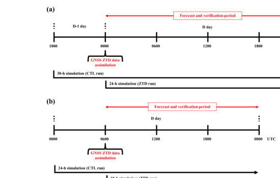
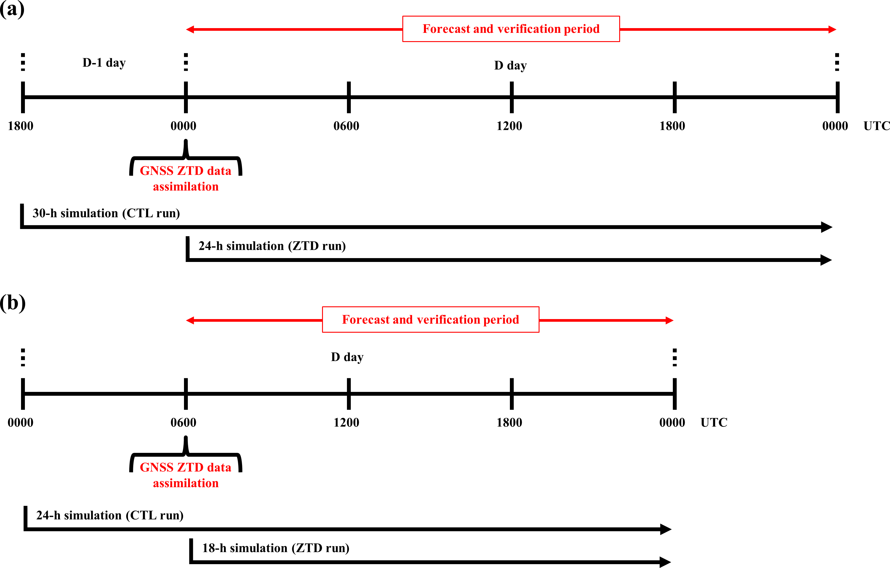
2.2.2. Numerical Experiments

Figure 2 illustrates the flow diagrams of the numerical experiments implemented in the current study. Two simulations were performed for each day of the examined events. The first one was carried out without assimilation and refers to the control (CTL) experiment. The second simulation refers to the GNSS ZTD observations assimilation (ZTD) experiment, in which the 3D-var/WRF system under cycling mode was employed. The criterion for selecting the time of ZTD data assimilation for the dry period events was mainly based on the approximate time of the actual start of the convective precipitation and it was set 6 h prior to this time. Τhus, data assimilation was applied at 0600 UTC for the May and July cases (Figure 2b), and at 0000 UTC for the June and August cases. For the wet season episodes, the 0000 UTC was chosen as the assimilation hour because the surface low-pressure systems were well developed at that time (Figure 1a).

2.3. ZTD Observations

GNSS applications in meteorology require careful characterization and assessment of tropospheric products derived from ground-based GNSS receivers. This is one of the key specialization areas for the GNSS Quality Control (GNSS-QC) team of the Aristotle University of Thessaloniki (AUTh), which processes and monitors a network of permanent GNSS stations located in Greece. The network consists of over 90 GNSS reference stations deployed by both public and private organizations. Four out of the 90 GNSS stations are included in the EUREF (European reference frame; [54]) permanent network (EPN). The GNSS-QC group has contributed to the E-GVAP project since 2014, providing NRT ZTD estimates to the European NWP centers [55,56,57].

In the current study, hourly ZTD observations, at 0000 UTC and 0600 UTC, of the AUTh GNSS-QC network were used for the WRF data assimilation experiments. The data collection and analysis were carried out for 2018 in the framework of BERTISS (Balkan-Mediterranean Real Time Severe Weather Service) project. An automated NRT processing scheme was employed using the Bernese software package, version 5.2 [58], and several coding scripts and algorithms for computations, data management, quality control, and database upload [15,59].

Since the observations accuracy and their associated errors is crucial in improving the model analysis, the quality control of the GNSS ZTD estimates and the appropriate treatment of ZTD formal errors within the 3D-var/WRF system are necessary. For this, a thorough observations pre-processing was applied in the present work to prepare the ZTD data for the assimilation process.

Data Pre-Processing

The accuracy of the NRT ZTDs, derived from the AUTh GNSS network, was examined by comparing the data against high-quality reference ZTD data provided by EPN. Based on the availability of the EPN weekly combined ZTD solutions, the validation was performed over the AUT1 station (Figure 1b) using concurrent data of the 2018 dataset. Following previous studies [60,61,62], the accuracy of the ZTD observations was defined as the standard deviation of the difference between the AUT1 and EPN ZTDs. The analysis resulted in an accuracy of 7.6 mm, which is between the optimal (5 mm) and target (10 mm) accuracy value according to the E-GVAP standards for NRT ZTDs used in the NWP models [63]. This outcome was a strong indication that the accuracy of the AUTh GNSS ZTD data was sufficient to assimilate them into the WRF modeling system.

Further, the observations in the 3D-var system are considered to have unbiased errors with respect to the WRF model. To meet this assumption, a statistical bias correction was applied to the ZTD data for each studied precipitation episode. More specifically, the differences between the observed and modeled ZTDs were computed for each GNSS receiver during a 10 day period prior to each event using the WRF simulations conducted for the model background errors covariance matrix specification (see Section 2.2.1). Then, the corrections were estimated as the mean values of the ZTD differences and they were subtracted from the ZTD observations that were lined up for data assimilation. Even though this method provides statistical corrections, this is a standard bias correction approach for ZTD data that proved to be successful in reducing the observations-model divergences and capturing the systematic errors between the ZTD observations and model forecasts [16,18,19,20,21,22,23,24,25,28]. The last stage of the ZTD data pre-processing included a selection algorithm based on the following conditions: (a) The formal ZTD error to be lower than the standard deviation of the difference between the observed and modeled ZTD, (b) the ZTD difference between observations and model output to be lower than five times the ZTD formal error, and (c) the difference between the receiver height and the model’s orography to be below 100 m. Similar criteria have been applied in previous studies [19,20,21,22,23,24,25]. Based on data availability and the above selection algorithm, the number of GNSS reference stations used per event ranged from 48 to 56. The assimilated ZTD observations had the same range, since assimilation was performed once (at 0000 UTC or 0600 UTC) during the conducted experiments. The locations of the 55 stations used for the event of 27 November 2019 are shown in Figure 1b, demonstrating a sufficient and homogeneous spatial coverage of the Greek territory.

2.4. Evaluation Process

Hourly precipitation measurements covering the entire study area were used to evaluate the model performance under both the CTL and ZTD numerical experiments. The data were collected from a dense network of weather stations operated by NOA [29]. In terms of data availability, different rain gauges were used for each case study. In total, 340 to 360 rain gauges were utilized for each rainfall event (Figure 1b). The observed and modeled precipitation data were paired in time and space, considering the nine nearest to the location of each rain gauge model grid points. The grid point having the closest predicted value to the observed one was selected for evaluation in order to avoid penalizing the model performance due to possible small spatial displacements of rainfall. The evaluation was performed for the 24 h and 6 h accumulated precipitation at 0000 UTC, 0600 UTC, 1200 UTC, and 1800 UTC.

Using the observation-model pairs, qualitative statistical measures were computed on the basis of a dichotomous application system (occurrence/no occurrence of precipitation) for six distinct rain thresholds: above 0.2, 1, 2, 5, 10, and 20 mm. The computed scores included the probability of detection (POD), the false alarm ratio (FAR), the equitable threat score (ETS), and the frequency bias (FBIAS). POD shows the fraction of observed events that were correctly modeled and ranges from zero (0: wrong forecast) to one (1: perfect forecast). FAR is the fraction of forecast events that were not observed and spans from zero (0: perfect forecast) to one (1: wrong forecast). ETS measures the skill of a model prediction considering the chance of randomly correct forecasts. ETS values close to unity (1) indicate a high-accuracy forecast, whereas ETS values that are close to zero (0), or even negative, shows a poor or random forecast quality. FBIAS is the ratio between the frequencies of forecasted and observed events and indicates whether a model tends to underestimate (FBIAS < 1) or overestimate (FBIAS > 1) the frequency of the occurrence of the observed events. To determine the statistical significance of the qualitative score differences between the conducted experiments, a hypothesis test approach was applied, using two confidence intervals: (i) 90% and (ii) 95%. The test was based on the construction of a probability density function that was consistent with the assumption that there was no difference between the qualitative statistical measures computed using the CTL simulations and those calculated based on the ZTD simulations. A brief description of the implemented method can be found in Giannaros et al. [64]. Quantitative statistical measures were also calculated, namely the mean bias (MB) and mean absolute error (MAE), for each precipitation threshold in order to account for the magnitude of errors. MB is used as a measure of the model tendency of rain underestimation (MB > 0) or overestimation (MB < 0), while MAE represents the absolute deviation between the observational and modeled precipitation. Following Giannaros et al. [64], the statistical significance of the MAE differences between the CTL and ZTD experiments was computed by applying the non-parametric Wilcoxon signed-rank test at the 90% and 95% confidence intervals. In addition to the statistical evaluation, the modeled differences concerning the rainfall distribution were thoroughly investigated for two events representing different synoptic conditions.

3. Results

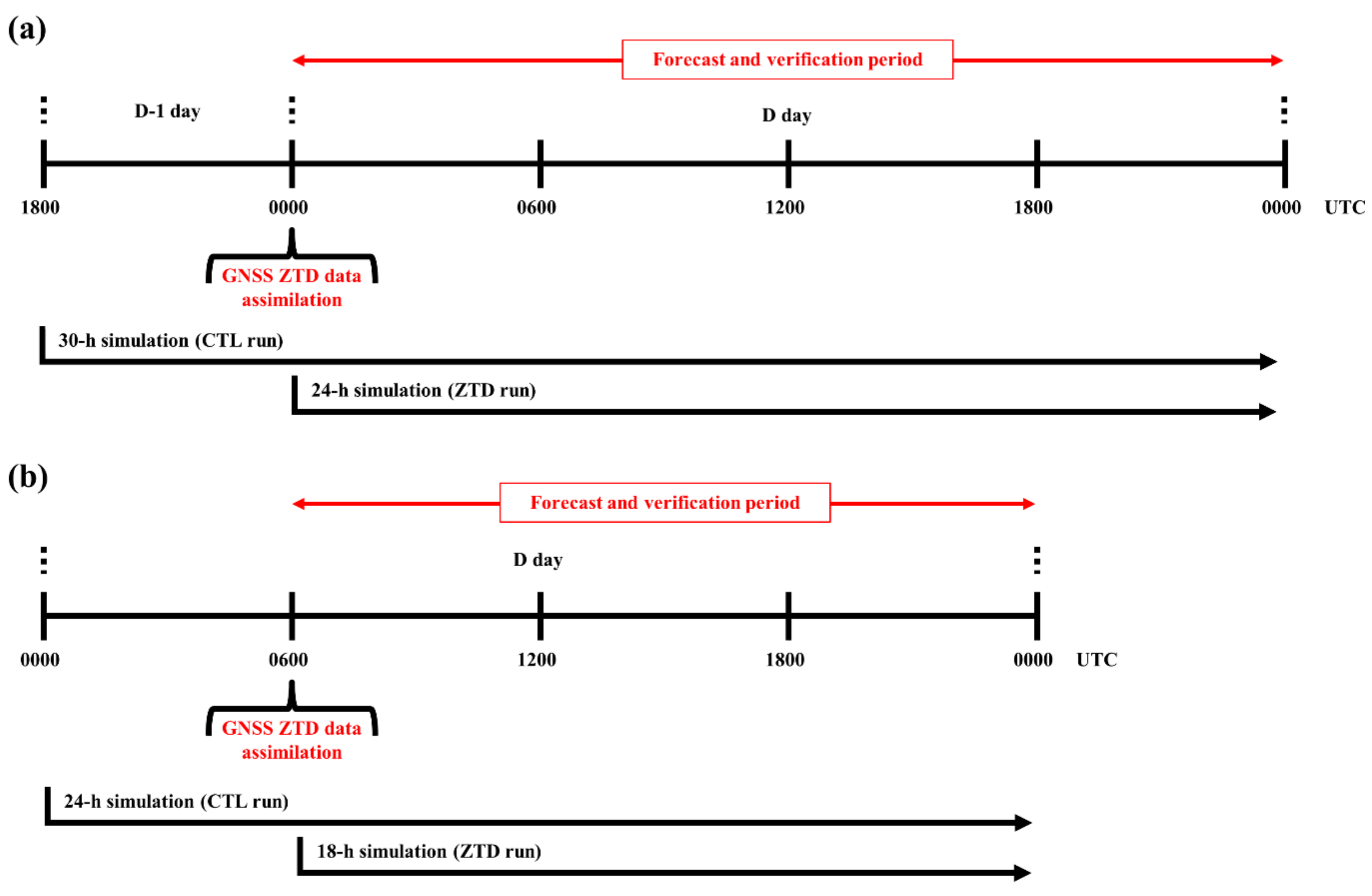
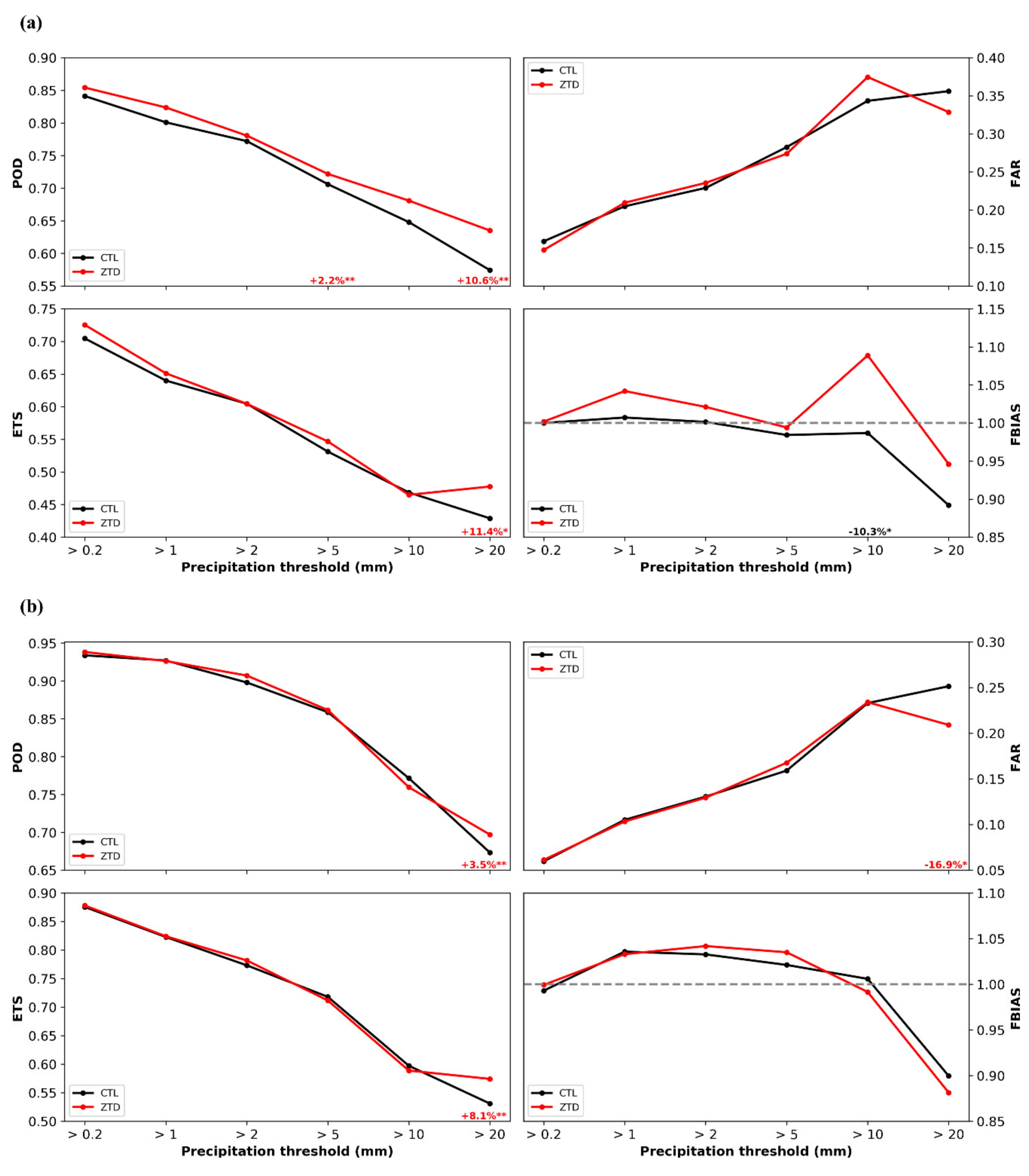
3.1. Statistical Evaluation

3.3.1. Daily Precipitation

Figure 3 presents the categorical scores for each 24 h accumulated precipitation threshold, aggregated for the dry and wet season rainfall events for the CTL and ZTD numerical experiments. Overall, the model performs adequately in capturing the occurrence (non-occurrence) of precipitation, as indicated by the POD (FAR), which is higher (lower) than 0.57 (0.38) and 0.67 (0.26) for all thresholds during the dry (Figure 3a) and wet (Figure 3b) period, respectively. The ETS values show a satisfying precipitation forecast quality, especially for the wet season (Figure 3b), when they range from 0.53 to 0.88. During both periods, the FBIAS values demonstrate that the model underestimates the observed frequency of higher than 20 mm daily precipitation, whereas it slightly overestimates the frequency of the observed daily rainfall for the lower than 20 mm thresholds, except those that are greater than 2 mm (5 mm and 10 mm) during the CTL experiment in the wet (dry) season (Figure 3).

Assimilating ZTD observations into the 3D-var/WRF model leads to increased probability of precipitation detection during the dry period (Figure 3a) across all rainfall thresholds. Especially for the highest precipitation threshold (>20 mm), the ZTD assimilation induced relative improvement is 10.6% (statistically significant at the 95% confidence interval; Figure 3a). Concerning FBIAS, the ZTD experiment leads to larger frequency biases compared to the CTL simulation, when precipitation is lower than 20 mm in the dry period, reaching 10.3% relative difference for the above 10 mm rainfall threshold (statistically significant at the 90% confidence interval; Figure 3a). FAR in the dry period is also higher for the same threshold (>10 mm) during the ZTD experiment, whereas a decrease in FAR is evident for greater than 20 mm 24 h precipitation when ZTD assimilation is applied (Figure 3a). No marked differences between the CTL and ZTD experiments are evident during the dry season for ETS, except from the considerable improvement by 11.4% (statistically significant at the 90% confidence interval) provided by the ZTD assimilation for the highest precipitation threshold (Figure 3a). For the same threshold, the ZTD experiment also leads to statistically significant improvements for all statistical measures, except FBIAS during the wet season (Figure 3b). In particular, POD and ETS are increased by 3.5% and 8.1% at the 95% confidence level, while FAR is reduced by 16.9% at the 90% confidence interval (Figure 3b).

In terms of quantitative statistics, the model overestimates, to a small extent, the 24 h accumulated precipitation values that are lower than 10 mm (20 mm) during the dry (wet) period, whereas it significantly underestimates the high rainfall accumulations for both dry and wet season events (Figure 4). More specifically, the CTL and ZTD mean absolute errors exceed 15 mm for the larger precipitation threshold, showing that both numerical experiments cannot capture the magnitude of severe rainfall (Figure 4). A similar extent of errors for intense precipitation thresholds have also been found in previous studies (e.g., see References [53,65,66]), showing that quantitative precipitation forecasting (QPF) remains a challenge for regional NWP systems due to uncertainties associated with physics parameterizations, primarily microphysics and convection, domain configuration (e.g., resolution and size), and initial conditions [67,68]. The improvement of a model’s initial state through data assimilation results in more accurate QPF. This is evident in the present study, as the ZTD simulations reduce the deviations from the observations in the precipitation interval [20,...) mm by ~1.10 mm during both dry and wet periods (Figure 4). In the latter season, this reduction corresponds to a 5.5% (statistically significant at the 95% confidence interval) relative improvement in MAE (Figure 4b). For the rest of the rainfall thresholds, lower (higher) ZTD MAEs can be seen between 2 (0 mm) and 20 mm (2 mm) of precipitation during the wet (dry) period (Figure 4).

3.3.2. 6 h Accumulated Precipitation

Further, the 6 h accumulated precipitation forecasts have been also verified in order to assess the impact of the ZTD data assimilation depending on the forecast lead time (Figure 5, Figure 6, Figure 7, Figure 8, Figure 9 and Figure 10). The statistical measures for the dry season were computed for the period between 0600 UTC and 1800 UTC. The periods from 0000-0600 UTC and 1800-0000 UTC were discarded from the analysis because less precipitation was observed and fewer observation-model pairs were available compared to the 0600–1800 UTC time window. Figure 5 and Figure 6 illustrate that the ZTD assimilation leads to a marked improvement of the precipitation forecasting in the dry season by increasing the probability of detection and the prediction quality. The improvement is more profound during the afternoon hours (12000–18000 UTC), when statistically significant increases at the 95% confidence level are evident for POD and ETS, which reach 27.8% for higher than 10 mm threshold and 21.4% for higher than 5 mm threshold, respectively (Figure 5b). In the same 6 h interval, the ZTD experiment results in higher FBIAS values, which are greater than 1 when rainfall is lower than 20 mm. This finding partially explains the overall overestimation of the observed events frequency found for the below 20 mm 24 h precipitation in the dry period (Figure 3a). FAR is mainly decreased during the ZTD experiment between 0600 and 1800 UTC in the dry period, especially for the higher rainfall threshold (Figure 5). This is also true for MAE, as shown in Figure 6. In particular, statistically significant reductions of 13% (19.9%) at the 95% (90%) confidence level are introduced by the ZTD simulation for precipitation above 20 mm (between 5 and 10 mm) from 1200–1800 (0600–1200) UTC (Figure 6). Figure 6 also illustrates that, when considering the lowest three rainfall thresholds (<5 mm), the WRF model mainly overestimates the observed precipitation, whereas it underestimates the higher than 5 mm observed rainfall during the examined forecast lead times. From 1200-1800 UTC, the model overestimation between 1 and 2 mm of precipitation is higher by 57.4% (statistically significant at the 90% confidence interval) during the ZTD simulation (Figure 6). The forecast errors for the rainfall thresholds up to 10 mm are smaller than ~9 mm for all 6 h intervals, while in contrast, they are greater than 19 mm for the highest precipitation threshold (Figure 6).

During the wet season (Figure 7, Figure 8, Figure 9 and Figure 10), the positive impact of ZTD assimilation on the 6 h accumulated precipitation, especially when exceeding 20 mm, is clearly shown. More specifically, during the first 6 h of the numerical forecasts, the FAR is decreased by 3.2% (statistically significant at the 95% confidence interval) for the highest rainfall threshold when ZTD data are assimilated in the WRF model (Figure 7a). For the same period and threshold, FBIAS is closer to 1 during the ZTD experiment, whereas no significant divergences between the conducted simulations are found for POD and ETS (Figure 7a). Marked differences are also not evident between 0600 UTC and 1200 UTC for all qualitative statistical measures and precipitation thresholds, except for POD, which is higher by 2.3% (statistically significant at the 95% confidence interval) during the ZTD experiment, when rainfall is above 5 mm (Figure 5b). From 1200-000 UTC, the POD and ETS scores are higher for the ZTD compared to the CTL experiment for the majority of the precipitation thresholds. Especially for the greater rainfall threshold, the improvement provided by the ZTD assimilation in POD and ETS is 10% in the intervals 1200-1800 UTC and 1800-0000 UTC, respectively (Figure 8). Additionally, a statistically significant (95% confidence level) reduction of ETS by 11% is evident during the ZTD simulation for the higher than 10 mm precipitation threshold between 1200 UTC and 1800 UTC (Figure 8a). Concerning the categorical statistical measures, the ZTD assimilation results in the increase of the MAE by ~1 mm (~12%) for the highest rainfall threshold from 0000–0600 UTC (Figure 9a). Statistically significant reductions by 5.4% (90% confidence level) and 8.5% (95% confidence level) provided by the ZTD experiment are found for the precipitation intervals [2,5) and [10,20) from 0000–0600 UTC and 0600–1200 UTC, respectively (Figure 9). MAE is also decreased by 8.4% (statistically significant at the 95% confidence interval) during the ZTD simulation when rainfall is greater than 20 mm in the 6 h forecast from 1200–1800 UTC (Figure 10a). For most of the lower than 20 mm precipitation thresholds, the ZTD simulation between 1200 and 0000 UTC provides improvement. The MB values show that the WRF model overestimates the three lowest rainfall thresholds, with error magnitudes lower than ~4 mm for all 6 h intervals. In contrast, the precipitation amounts that are higher than 5 mm are underestimated by the model and the extent of under-prediction increases with the forecast lead time (Figure 9 and Figure 10).

3.2. Analysis of Selected Case Studies

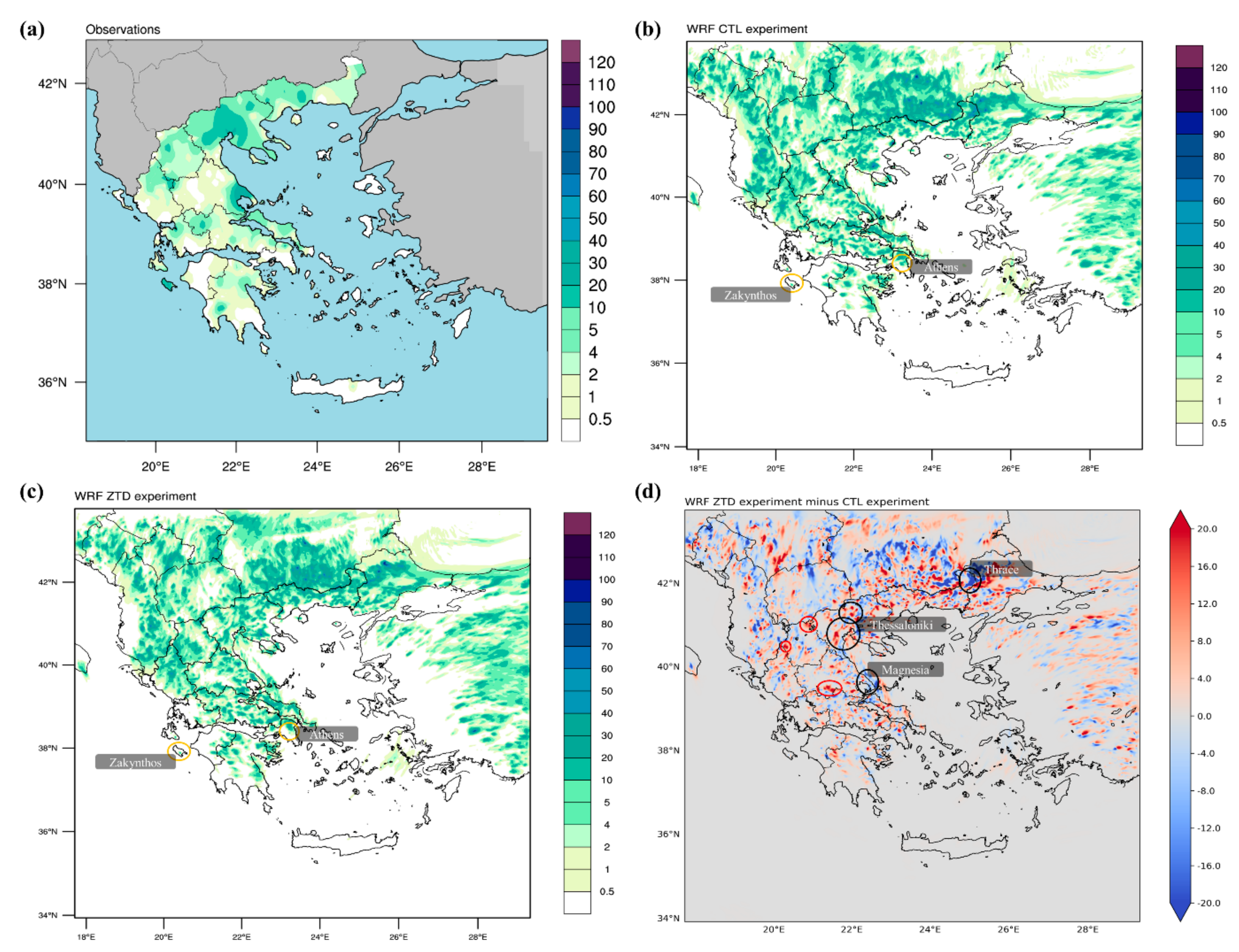
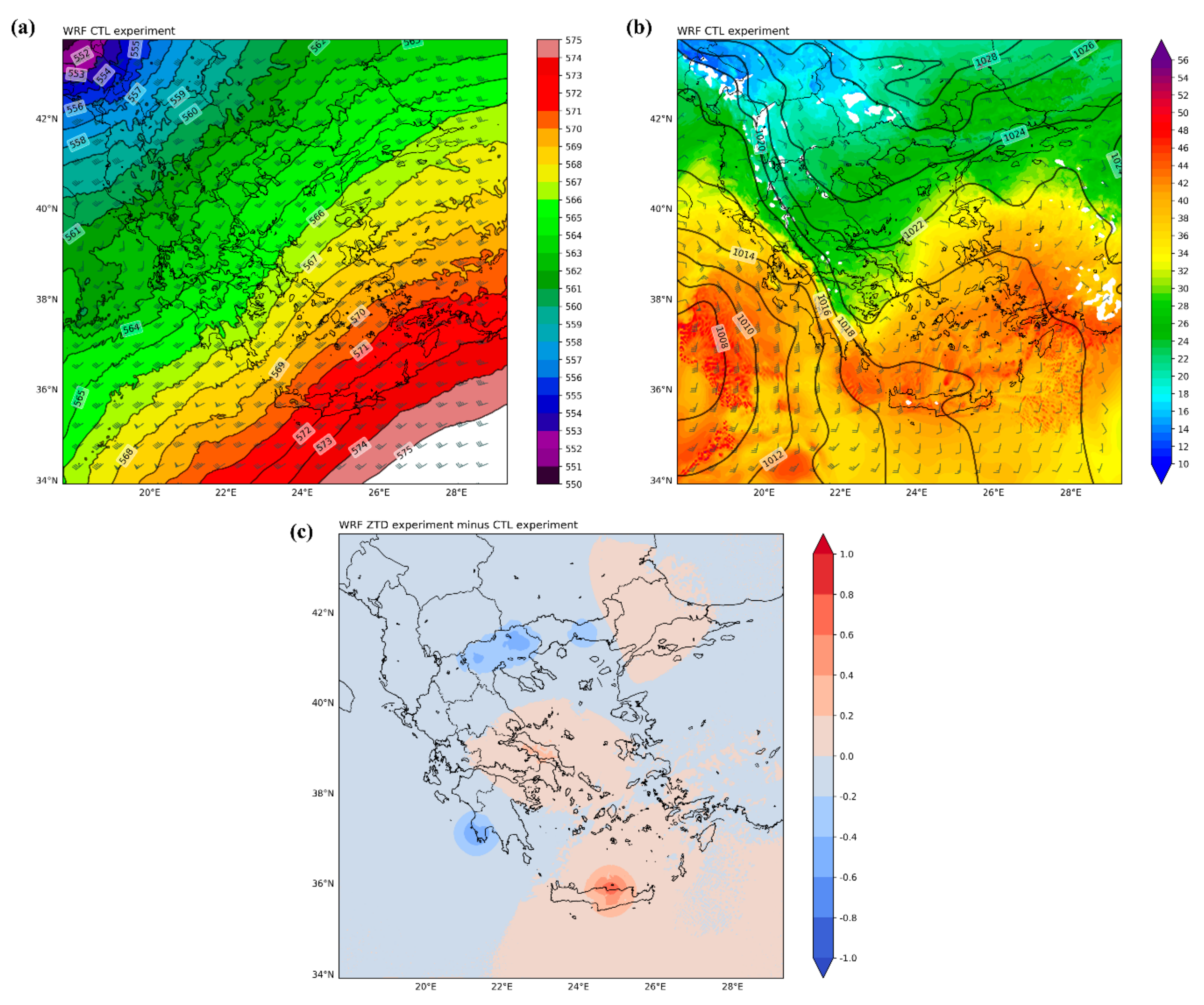
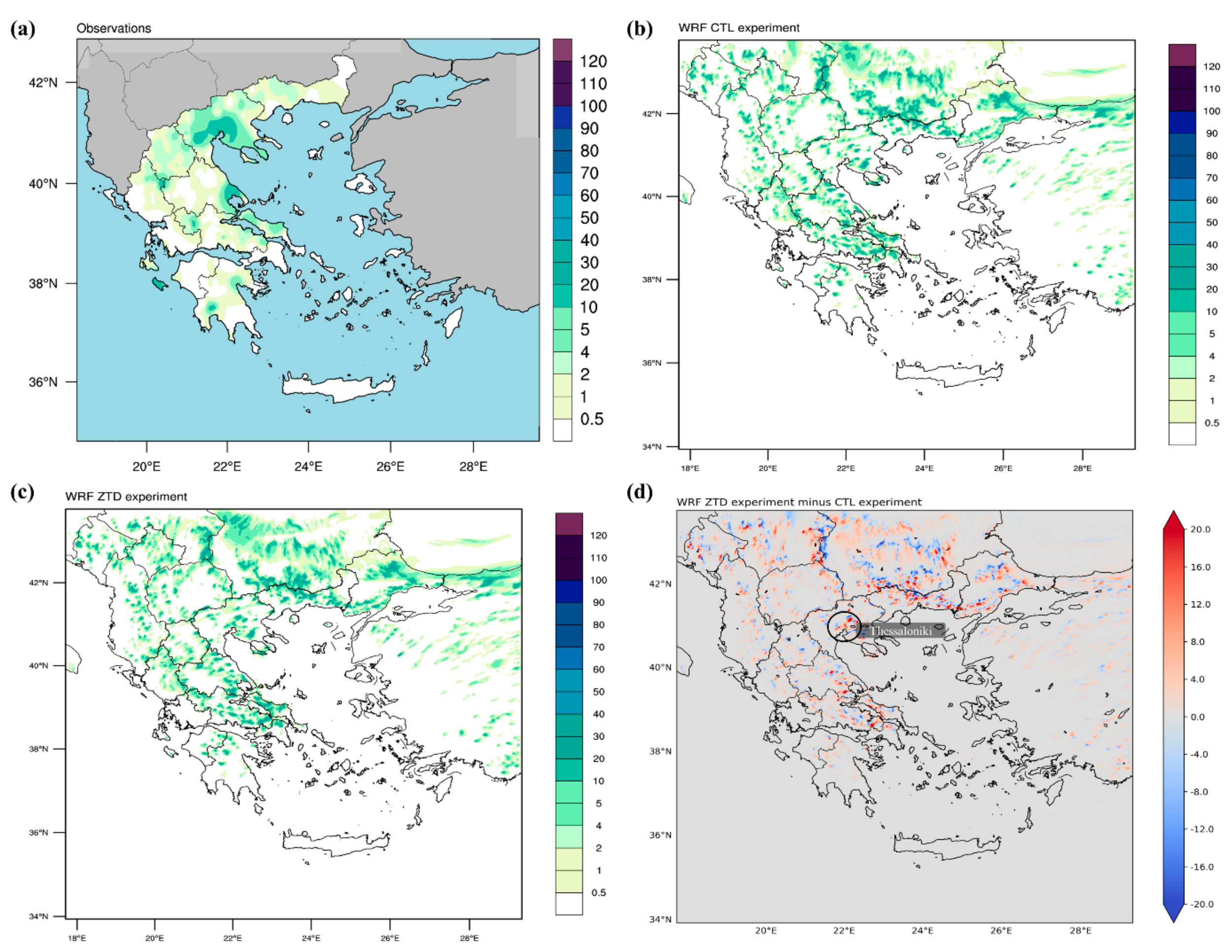
3.2.1. 10 May 2018

Figure 11a–b illustrate the atmospheric conditions at 0600 UTC, as simulated by the CTL experiment. As seen in the 500 hPa geopotential height and wind (Figure 11a), Greece is affected by a cyclonic atmospheric circulation in the middle troposphere, with a cut-off low over Western and central Greece. The cold air pool aloft is accompanied by a surface low over the central part of the country (Figure 11b). These synoptic conditions typically occur during late spring in Greece, producing strong atmospheric instability, which in turn results in intense convective activity. Figure A1 shows that, when ZTD data are assimilated into the WRF model, the modeled circulation pattern is the same as in the CTL experiment (Figure 11a–b). However, a discrete displacement of the 500 hPa geopotential height and sea level pressure gradients is evident, demonstrating the modification of the initial conditions by the ZTD assimilation at the time of the ZTD experiment initialization (0600 UTC). Since ZTD is related to precipitable water (PW), the initial conditions alteration at 0600 UTC is also evident for the modeled PW, as shown in Figure 11c. The initial PW differences between the conducted experiments emerge in locations where GNSS stations are situated (Figure 11c and Figure 1b).

The modification of the initial conditions of the ZTD experiment, due to the ZTD data assimilation, leads to differences in precipitation forecasts, as illustrated in Figure 12. In particular, the ZTD simulation (Figure 12c) improves the reproduction of the observed daily precipitation (Figure 12a) intensity and spatial distribution over the two high-rainfall regions, namely Thessaloniki and Magnesia. As presented in Figure 12d, with the black circles, higher precipitation amounts are simulated by the ZTD experiment over the city of Thessaloniki, as well as over the Western and Northern parts of the region. The ZTD assimilation also leads to greater (lower) daily rainfall values that are closer to the observations over the Northern (Southern) part of the Magnesia region (highlighted by the black circle in Figure 12d). Moreover, the assimilation of ZTD data into the WRF model results in the reduction of the significant precipitation overestimation produced by the CTL simulation over Northeast Thrace (Figure 12d). However, the ZTD experiment simulates considerably higher daily precipitation accumulations compared to the observations and CTL experiment over some regions, such as those highlighted by red circles in Figure 12d (e.g., central Greece). Overall, the model performs adequately in capturing the observed rainfall distribution over Greece, except the Zakynthos and Athens regions (orange circles in Figure 12b–c), where both CTL and ZTD simulations fail to reproduce the precipitation amounts, even though it is worth mentioning that the ZTD experiment reduces the geographical extent of the false forecast over the Athens area. The improvement in the reproduction of the observed rainfall when ZTD data are assimilated into the WRF model is also evident in the diurnal precipitation cycle analysis. As indicatively shown in Figure A2, most of the daily rain over the Thessaloniki region was observed between 0600 UTC and 1200 UTC, with the ZTD experiment simulating notably higher precipitation amounts (Figure A2d), which is in better agreement with the observations (Figure A2a).

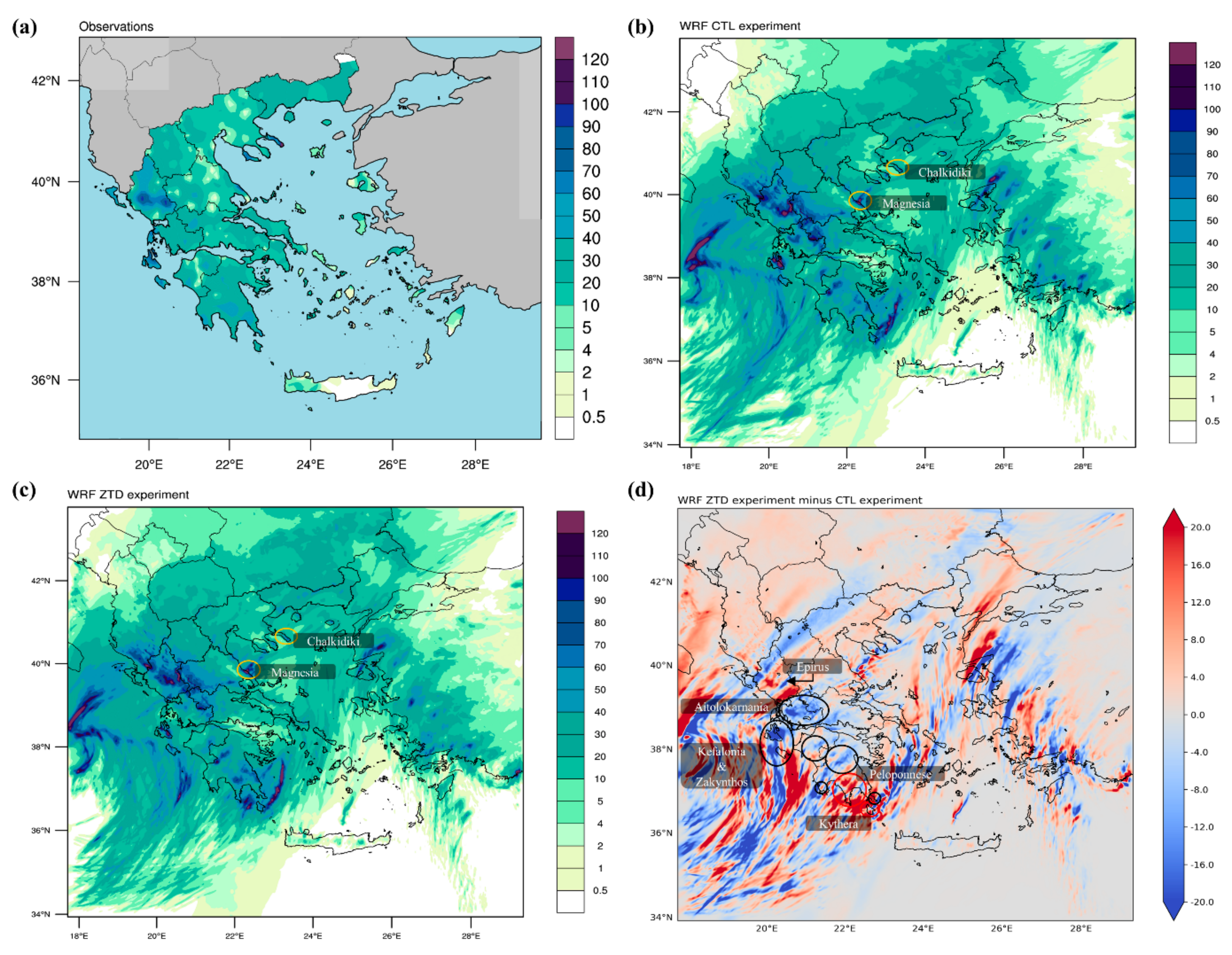
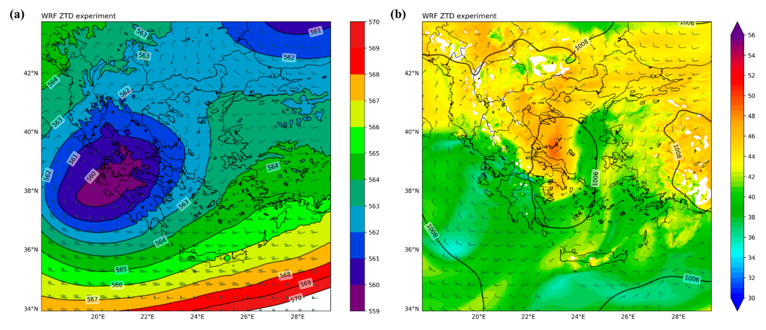
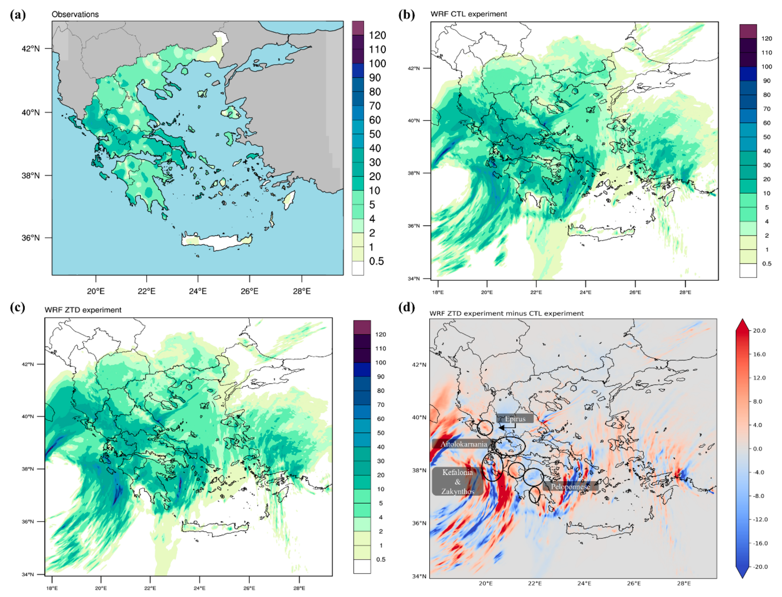
3.2.2. 18 November 2018

During the selected wet period event, Greece was affected by a deep surface low-pressure system. As shown in the sea-level pressure and 850 hPa equivalent potential temperature and wind fields (Figure 13b), the surface low is located over the Southwest Ionian Sea at 0000 UTC on 18 November, resulting in very strong Southerly winds. During the next hours, as the surface low is moving Northeast, the Southwesterly flow advects warm and moist air over Greece (Figure A3a–b). As in the case of the dry season event (see Section 3.2.1), both CTL and ZTD experiments simulate the same atmospheric conditions with slight differences in the 500 hPa geopotential height and sea level pressure gradients (Figure A4) at the ZTD experiment initialization time (0000 UTC). Again, the impact introduced by the ZTD data assimilation is clearly evident in the initial PW field at 0000 UTC (Figure 13c). The PW differences at 0000 UTC between the two experiments arise again over locations where GNSS stations are found (Figure 1b), but a more complicated pattern is evident in this case study.

Similarly, the 24 h modeled precipitation differences between the CTL and ZTD simulations arising from the modification of the initial conditions of the ZTD experiment due to the ZTD assimilation are more complex and widespread during this event (Figure 14d). The most noticeable differences are found over Western Greece, where the highest rainfall amounts were observed (Figure 14a). In particular, as shown in Figure 14d with black circles, the ZTD experiment produces lower (higher) precipitation over Kefalonia Island, the Aitolokarnania region, and central Peloponnese (the center of Zakynthos island, and Southwest and Southeast Peloponnese) compared to the CTL simulation, more accurately representing the observed rainfall. A more accurate reproduction of the precipitation observations by the ZTD experiment is also evident in Northwest Peloponnese, while in contrast, the ZTD assimilation leads to a more pronounced overestimation of the observed rainfall over central–North Peloponnese and Kythera Island, as indicated by the red circles in Figure 14d. Mixed results are found over the Epirus region, where the ZTD (CTL) experiment forecasts a rainfall pattern that is closer to the observed one in the central and Northern (Southern) part of the area. Overall, the model lacks the ability to capture the magnitude of observations, especially for intense precipitation, as shown by the notable underestimation (overestimation) of the observed rainfall over the area denoted by the orange circle in Chalkidiki (Magnesia) region in Figure 14b–c. However, the spatial distribution of the observed precipitation is well captured by both CTL and ZTD simulations. The above findings are also evident when examining the diurnal precipitation cycle in 6 h intervals and highlight the good performance of the WRF model in reproducing the temporal distribution of the observed rainfall, especially during the ZTD experiment. Indicatively, both simulations (Figure A5b–c) adequately replicate the observed spatial pattern of the precipitation between 0600 and 1200 UTC (Figure A5a), with the ZTD experiment improving the rainfall amounts forecasts over North Epirus, Aitolokarnania and Peloponnese regions, and Kefalonia and Zakynthos Islands (Figure A5d).

4. Discussion

The results presented above demonstrate a beneficial impact of ZTD assimilation on the daily precipitation forecasts over Greece during both dry and wet periods (Figure 3 and Figure 4). This impact is more profound for heavy precipitation (>20 mm), for which statistically significant (at least at the 90% confidence level) improvements are provided by the ZTD assimilation concerning the probability of detection, the false alarm ratio, the quality of forecasts (ETS), and the magnitude of errors (MAE). This finding is of great importance as higher rainfall amounts are associated with more severe impacts, especially over the Mediterranean regions [20]. In general, the positive impacts of ZTD assimilation are more evident during the dry period. However, notable and statistically significant enhancements in the WRF model’s performance are also found during the ZTD experiment for both 24 h (Figure 3 and Figure 4) and 6 h precipitation (Figure 7, Figure 8, Figure 9 and Figure 10). This fact reflects a significant added value of ZTD assimilation during wet season rainfall events, in contrast with previous studies, which concluded that when the atmospheric state is well described during large synoptic-scale cases, no further improvement of the forecast accuracy can be achieved by assimilating ZTD observations (e.g., Boniface et al. [24]). Moreover, the ZTD assimilation substantially advances the overall model performance in terms of qualitative and quantitative rainfall forecasting between 0600 and 1800 UTC in the dry season (Figure 5 and Figure 6). Especially from 1200–1800 UTC, statistically significant (at the 95% confidence interval) higher POD, ETS, and MAE values, compared to the CTL experiment, are found across all precipitation thresholds. This is a key outcome considering that convective precipitation in the dry season mainly occurs during the examined time window and its forecasting is challenging, as NWP models lack the ability to resolve small-scale convective circulation [68,69]. In contrast, NWP models are more capable in dealing with large-scale dynamically-driven precipitation systems during the wet season [70]. This is evident in the current study because the WRF model, overall, performs better in the wet compared to the dry period. The case study analysis shows that ZTD assimilation provides a more accurate representation of the observed precipitation geographical extent in terms of 24 h and 6 h rainfall (Figure 12 and Figure A2 in the dry period and Figure 14 and Figure A5 in the wet period). It also highlights that the overall WRF performance improvement in rainfall forecasting under the ZTD experiment is due to the modification of the model’s initial conditions at the time of the experiment’s initialization through the assimilation of ZTD observations. The introduction of ZTD data assimilation especially affects the initial PW field, leading to noticeable differences between the conducted experiments, which emerge in locations where GNSS stations are found. This is evident in Figure 11c and Figure 13c concerning the selected case studies, as well as in Figure A6, Figure A7, Figure A8, Figure A9, Figure A10, Figure A11, Figure A12 and Figure A13, illustrating the PW differences between the CTL and ZTD simulations at the ZTD experiment initialization time for each day of the rest of the rainfall events examined in the present study.

5. Conclusions

The present work focuses on investigating the impact of assimilating GNSS ZTD observations on the WRF model precipitation forecast skill. The conducted work is the first attempt at applying ZTD data assimilation into a regional atmospheric model over Greece. The evaluation of the impact of ZTD assimilation is performed for seven high-impact rainfall episodes that occurred during the dry (four events) and wet period (three events) of 2018. A substantial effort was devoted to the pre-processing of ZTD observations in order to qualify their adequacy for data assimilation. Then, two sets of model experiments (CTL and ZTD) were performed and the model predicted rainfall was verified against observations, which were collected from over 330 rain gauges provided by the weather monitoring network of the National Observatory of Athens.

The qualitative and quantitative statistical evaluation provides substantial findings on how the assimilation of ZTD observations into the WRF model affects its performance:

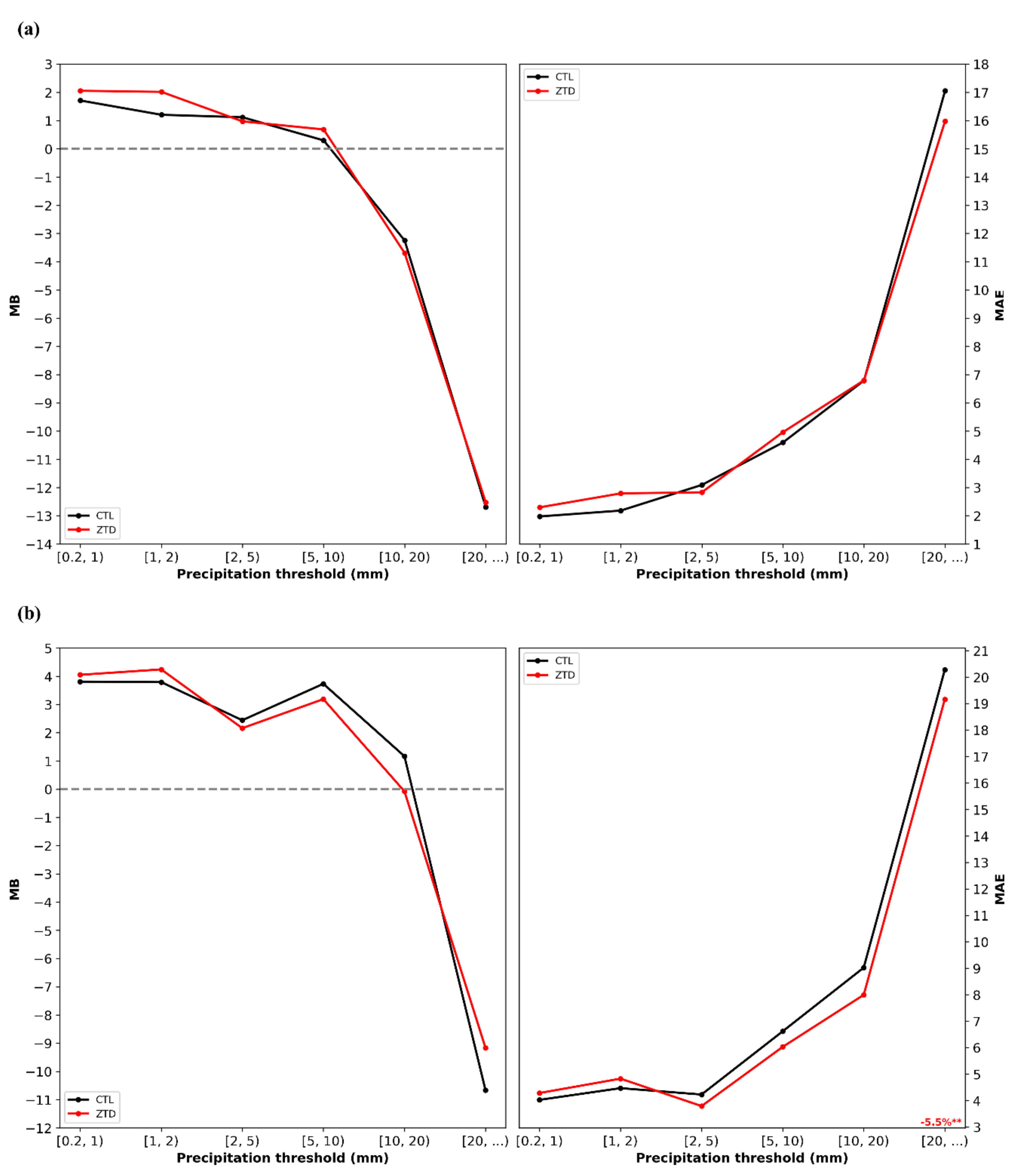
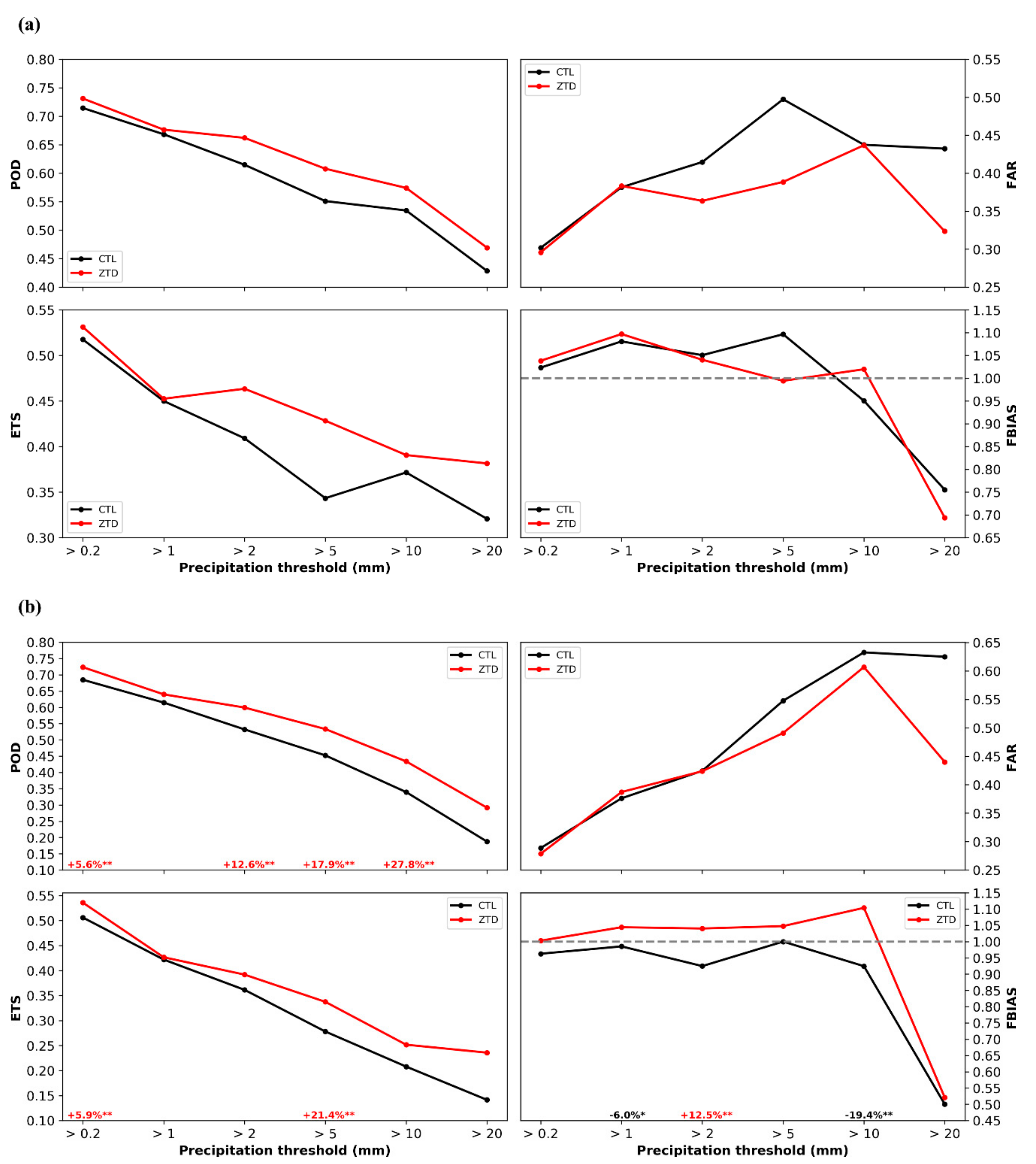
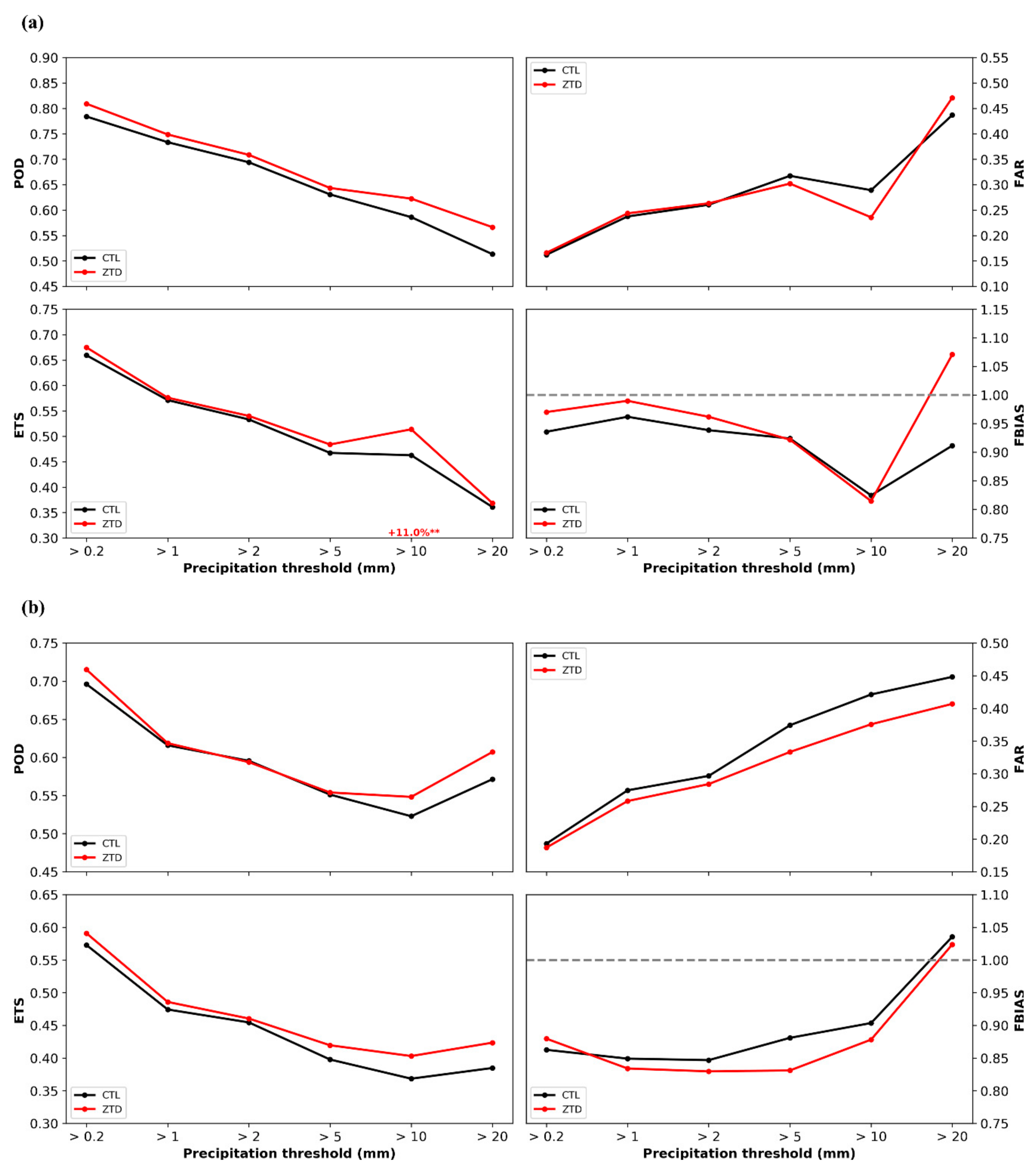
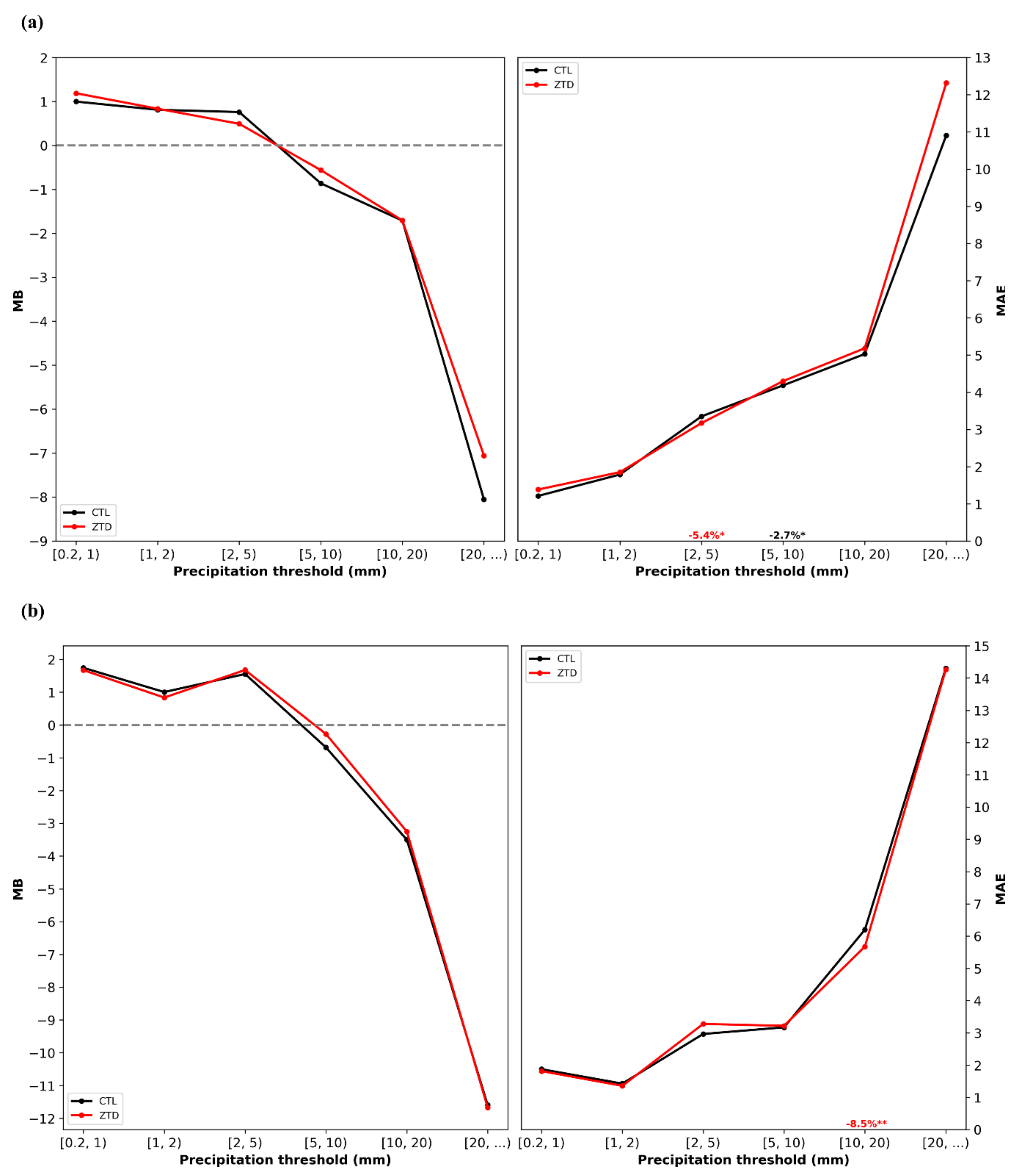
• The ZTD assimilation results into statistically significant (a)more accurate reproduction of the occurrence of the observed precipitation (higher POD by 10.6% and 3.9% in the dry and wet season, respectively), (b) reduction of the false forecasts (lower FAR by 7.7% and 16.9% in the dry and wet season, respectively), (c) better prediction quality (greater ETS by 11.4% and 8.1% in the dry and wet season, respectively), and (d) decrease in the magnitude of errors (lower MAE by 6.3% and 5.5% in the dry and wet season, respectively), compared to the CTL configuration, for intense rainfall (>20 mm). This outcome is of great importance when considering that heavy precipitation amounts are associated with greater impacts and may be poorly forecasted.
• The overall model performance enhancement in rainfall forecasting during the ZTD experiment is more evident in the dry season. However, the assimilation of ZTDs also leads to notable and statistically significant improvements during the wet period, indicating, in contrast to past studies, that it can provide a positive influence under large-scale synoptic conditions.
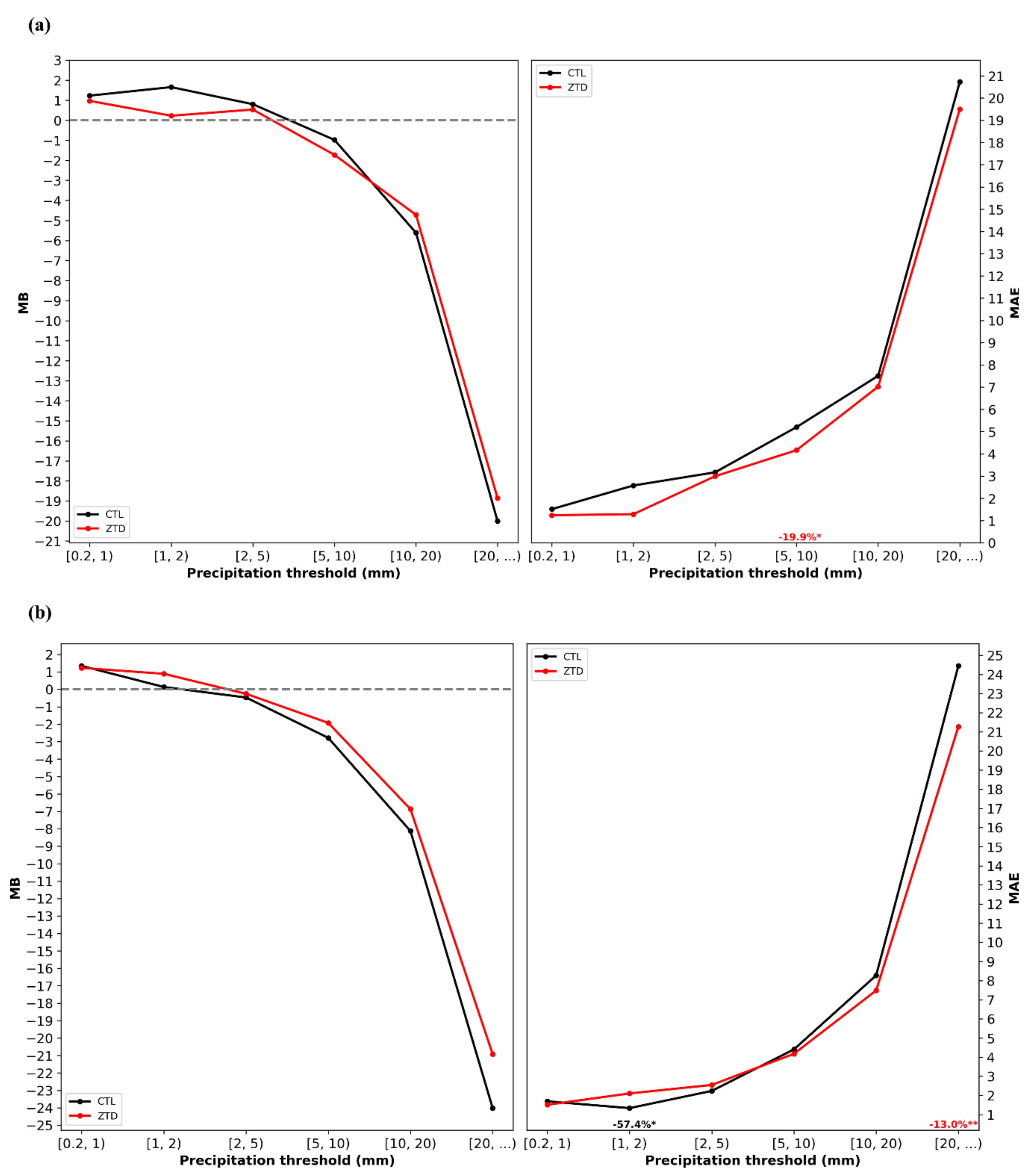
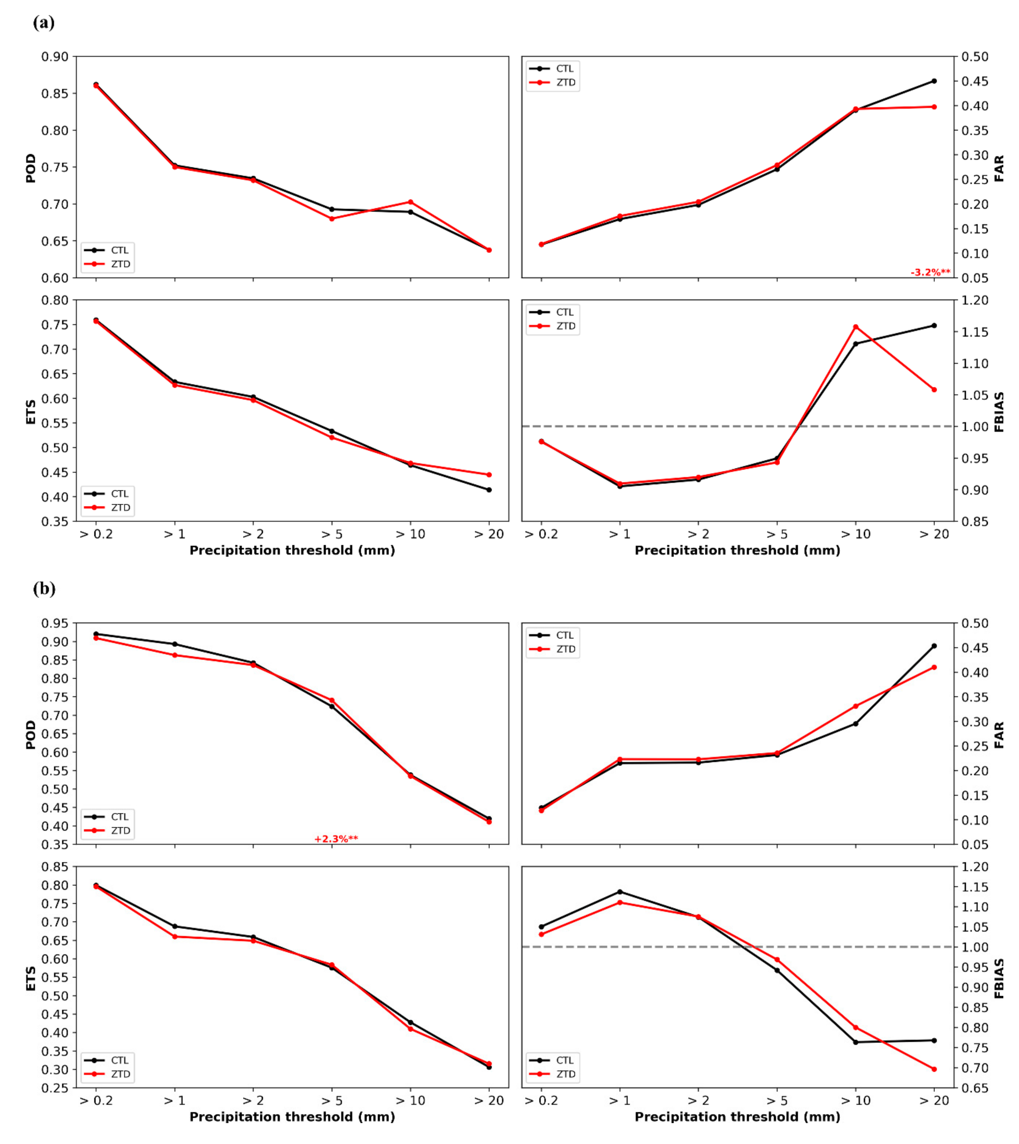
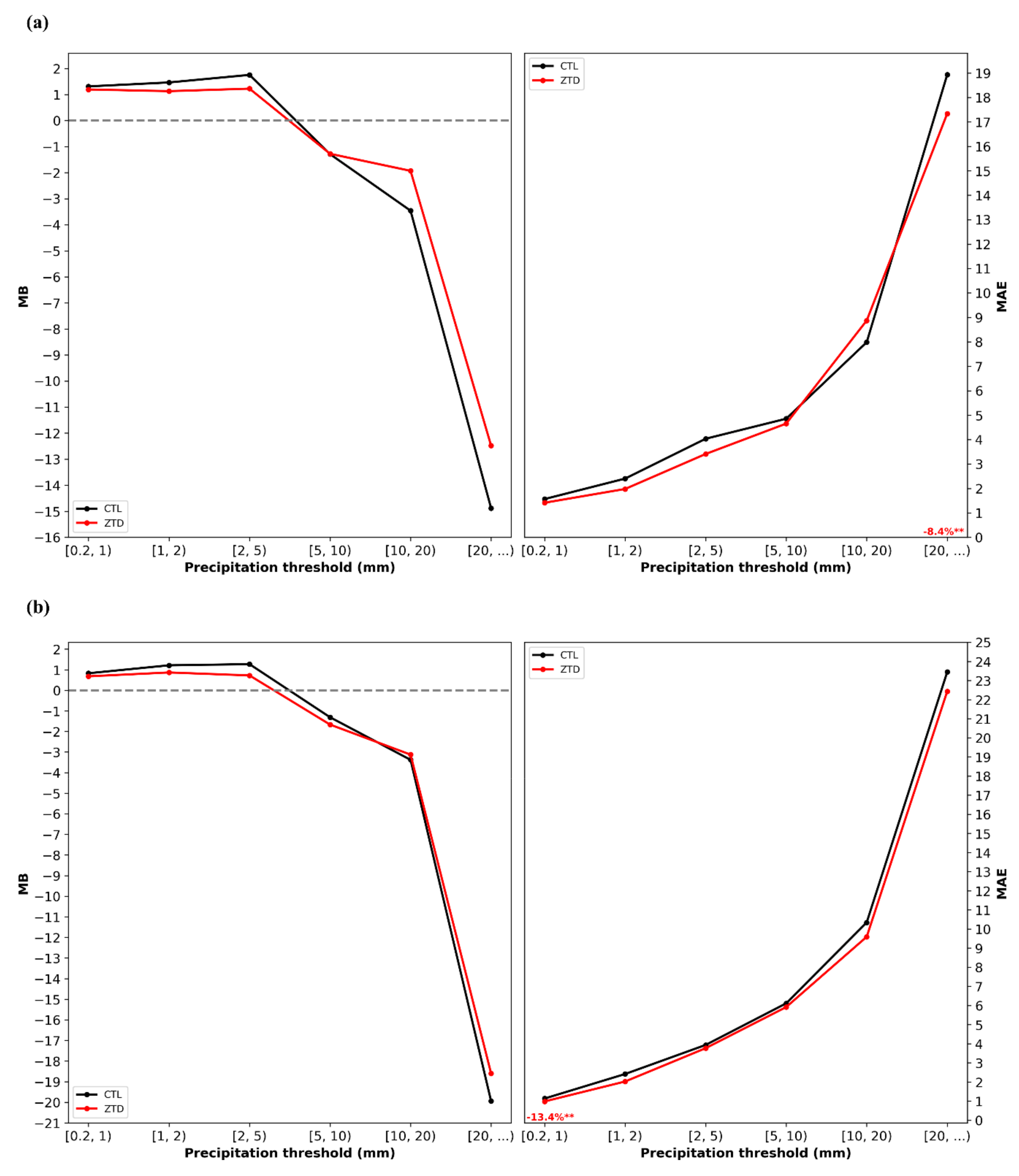
• The introduction of ZTDs into the WRF model induces statistically significant improvements in precipitation forecasts, especially for above 20 mm 6 h accumulations, during the time window (0600 to 1800 UTC) of convective rain occurrence in the dry season. This finding is essential as correctly forecasting high precipitation convective events during the dry period is crucial in issuing improved severe rainfall warnings.

The detailed presentation of two case studies (on 10 May and 18 November, 2018) show that the WRF model is capable of satisfactorily capturing the spatial and temporal distribution of the observed rainfall, with the ZTD simulation providing results that are closer to the observations. It also reveals that the precipitation forecast improvement under the ZTD experiment is induced by the initial conditions’ modification at the experiment’s initialization time, especially affecting the initial PW field, due to the ZTD assimilation.

The above findings highlight the beneficial impact of assimilating ZTD observations into high-resolution regional scale weather forecasting systems. It is the authors’ intention to investigate the impact of variational ZTD bias correction techniques and of ZTD spatiotemporal error correlations in the assimilation framework.

References

1. Sabatini, R.; Moore, T.; Ramasamy, S. Global navigation satellite systems performance analysis and augmentation strategies in aviation. Prog. Aerosp. Sci. 2017, 95, 45–98. [Google Scholar] [CrossRef]
2. Kubo, N.; Higuchi, M.; Takasu, T.; Yamamoto, H. Performance evaluation of GNSS-based railway applications. In Proceedings of the 2015 International Association of Institutes of Navigation World Congress (IAIN), Prague, Czech Republic, 20–23 October 2015; pp. 1–8. [Google Scholar]
3. Molina, P.; Colomina, I.; Vitoria, T.; Silva, P.F.; Skaloud, J.; Kornus, W.; Prades, R.; Aguilera, C. Searching Lost People with Uavs: The System and Results of the Close-Search Project. ISPRS Int. Arch. Photogramm. Remote Sens. Spat. Inf. Sci. 2012, 39, 441–446. [Google Scholar] [CrossRef] [Green Version]
4. Kahveci, M. Contribution of GNSS in precision agriculture. In Proceedings of the 2017 8th International Conference on Recent Advances in Space Technologies (RAST), Istanbul, Turkey, 19–22 June 2017; pp. 513–516. [Google Scholar]
5. Ostolaza, J.; Lera, J.J.; Pérez, D.; Cueto-Felgueroso, G.; Cueto, M.; Cezón, A.; Fernández, M.A.; López, M.; Hill, D.; Boissinot, V.; et al. Maritime Trials in Europe and Africa Using GNSS-based Enhanced Systems. In Proceedings of the 29th International Technical Meeting of the Satellite Division of The Institute of Navigation, Portland, OR, USA, 12–16 September 2016. [Google Scholar]
6. Guerova, G.; Jones, J.; Douša, J.; Dick, G.; De Haan, S.; Pottiaux, E.; Bock, O.; Pacione, R.; Elgered, G.; Vedel, H.; et al. Review of the state of the art and future prospects of the ground-based GNSS meteorology in Europe. Atmos. Meas. Tech. 2016, 9, 5385–5406. [Google Scholar] [CrossRef] [Green Version]
7. Bevis, M.; Businger, S.; Herring, T.A.; Rocken, C.; Anthes, R.A.; Ware, R.H. GPS meteorology: Remote sensing of atmospheric water vapor using the global positioning system. J. Geophys. Res. 2012, 97, 15787. [Google Scholar] [CrossRef]
8. Suparta, W.; Adnan, J.; Mohd Ali, M.A. Nowcasting the lightning activity in Peninsular Malaysia using the GPS PWV during the 2009 inter-monsoons. Ann. Geophys. 2014, 57, 0217. [Google Scholar]
9. Dousa, J.; Vaclavovic, P. Real-time zenith tropospheric delays in support of numerical weather prediction applications. Adv. Space Res. 2014, 53, 1347–1358. [Google Scholar] [CrossRef]
10. Hanna, N.; Trzcina, E.; Möller, G.; Rohm, W.; Weber, R. Assimilation of GNSS tomography products into WRF using radio occultation data assimilation operator. Atmos. Meas. Tech. Discuss. 2019, 12, 4829–4848. [Google Scholar] [CrossRef]
11. Simeonov, T.; Sidorov, D.; Teferle, F.N.; Milev, G.; Guerova, G. Evaluation of IWV from the numerical weather prediction WRF model with PPP GNSS processing for Bulgaria. Atmos. Meas. Tech. Discuss. 2016. [Google Scholar] [CrossRef] [Green Version]
12. Manning, T.; Zhang, K.; Rohm, W.; Choy, S. Detecting Severe Weather using GPS Tomography: An Australian Case Study. J. Glob. Position. Syst. 2012, 11, 58–70. [Google Scholar] [CrossRef]
13. Pikridas, C. Monitoring Climate Changes on Small Scale Networks Using Ground Based GPS and Meteorological Data. Artif. Satell. 2014, 49, 125–135. [Google Scholar] [CrossRef] [Green Version]
14. Pikridas, C. The use of GNSS tropospheric products for climate monitoring. A case study in the area of Ioannina Northwestern Greece. South East. Eur. J. Earth Obs. Geomat. 2015, 4, 81–90. [Google Scholar]
15. Pikridas, C.; Fotiou, A.; Bitharis, S.; Karolos, I.; Balidakis, K. BeRTISS: Balkan-Mediterranean real time severe weather service. The case of Greece. In Proceedings of the 5th International Conference on Civil Protection & New Technologies, Kozani, Greece, 31 October–3 November 2018. [Google Scholar]
16. Arriola, J.S.; Lindskog, M.; Thorsteinsson, S.; Bojarova, J. Variational bias correction of GNSS ZTD in the HARMONIE modeling system. J. Appl. Meteorol. Climatol. 2016, 55, 1259–1276. [Google Scholar] [CrossRef]
17. E-GVAP. Available online: http://egvap.dmi.dk/ (accessed on 24 January 2019).
18. Poli, P.; Moll, P.; Rabier, F.; Desrozier, G.; Chapnik, B.; Berre, L.; Healy, S.B.; Andersson, E.; El Guelai, F.Z. Forecast impact studies of zenith total delay data from European near real-time GPS stations in Météo France 4DVAR. J. Geophys. Res. Atmos. 2007, 112, 47. [Google Scholar] [CrossRef]
19. Yan, X.; Ducrocq, V.; Jaubert, G.; Brousseau, P.; Poli, P.; Champollion, C.; Flamant, C.; Boniface, K. The benefit of GPS zenith delay assimilation to high-resolution quantitative precipitation forecasts: A case-study from COPS IOP 9. Q. J. R. Meteorol. Soc. 2009, 135, 1788–1800. [Google Scholar] [CrossRef]
20. Yan, X.; Ducrocq, V.; Poli, P.; Hakam, M.; Jaubert, G.; Walpersdorf, A. Impact of GPS zenith delay assimilation on convective-scale prediction of Mediterranean heavy rainfall. J. Geophys. Res. Atmos. 2009, 114, 20. [Google Scholar] [CrossRef] [Green Version]
21. Eresmaa, R.; Salonen, K.; Järvinen, H. An observing-system experiment with ground-based GPS zenith total delay data using HIRLAM 3D-Var in the absence of satellite data. Q. J. R. Meteorol. Soc. 2010, 136, 1289–1300. [Google Scholar] [CrossRef]
22. Bennitt, G.V.; Jupp, A. Operational Assimilation of GPS Zenith Total Delay Observations into the Met Office Numerical Weather Prediction Models. Mon. Weather Rev. 2012, 140, 2706–2719. [Google Scholar] [CrossRef]
23. Schwitalla, T.; Bauer, H.-S.; Wulfmeyer, V.; Aoshima, F. High-resolution simulation over central Europe: Assimilation experiments during COPS IOP 9c. Q. J. R. Meteorol. Soc. 2011, 137, 156–175. [Google Scholar] [CrossRef]
24. Boniface, K.; Ducrocq, V.; Jaubert, G.; Yan, X.; Brousseau, P.; Masson, F.; Champollion, C.; Chéry, J.; Doerflinger, E. Impact of high-resolution data assimilation of GPS zenith delay on Mediterranean heavy rainfall forecasting. Ann. Geophys. 2009, 27, 2739–2753. [Google Scholar] [CrossRef]
25. Bennitt, G.V.; Johnson, H.R.; Weston, P.P.; Jones, J.; Pottiaux, E. An assessment of ground-based GNSS Zenith Total Delay observation errors and their correlations using the Met Office UKV model. Q. J. R. Meteorol. Soc. 2017, 143, 2436–2447. [Google Scholar] [CrossRef]
26. Macpherson, S.; Laroche, S. Estimation of ground-based GNSS Zenith Total Delay temporal observation error correlations using data from the NOAA and E-GVAP networks. Q. J. R. Meteorol. Soc. 2019, 145, 513–529. [Google Scholar] [CrossRef]
27. Mile, M.; Benáček, P.; Rózsa, S. The use of GNSS zenith total delays in operational AROME/Hungary 3D-Var over a central European domain. Atmos. Meas. Tech. 2019, 12, 1569–1579. [Google Scholar] [CrossRef] [Green Version]
28. Rohm, W.; Guzikowski, J.; Wilgan, K.; Kryza, M. 4DVAR assimilation of GNSS zenith path delays and precipitable water into a numerical weather prediction model WRF. Atmos. Meas. Tech. 2019, 12, 345–361. [Google Scholar] [CrossRef] [Green Version]
29. Lagouvardos, K.; Kotroni, V.; Bezes, A.; Koletsis, I.; Kopania, T.; Lykoudis, S.; Mazarakis, N.; Papagiannaki, K.; Vougioukas, S. The automatic weather stations NOANN network of the National Observatory of Athens: Operation and database. Geosci. Data J. 2017, 4, 4–16. [Google Scholar] [CrossRef]
30. Papagiannaki, K.; Lagouvardos, K.; Kotroni, V. A database of high-impact weather events in Greece: A descriptive impact analysis for the period 2001–2011. Nat. Hazards Earth Syst. Sci. 2013, 13, 727–736. [Google Scholar] [CrossRef]
31. Michaelides, S.; Karacostas, T.; Sánchez, J.L.; Retalis, A.; Pytharoulis, I.; Homar, V.; Romero, R.; Zanis, P.; Giannakopoulos, C.; Bühl, J.; et al. Reviews and perspectives of high impact atmospheric processes in the Mediterranean. Atmos. Res. 2018, 208, 4–44. [Google Scholar] [CrossRef]
32. Galanaki, E.; Kotroni, V.; Lagouvardos, K.; Argiriou, A. A ten-year analysis of cloud-to-ground lightning activity over the Eastern Mediterranean region. Atmos. Res. 2015, 166, 213–222. [Google Scholar] [CrossRef]
33. Kotroni, V.; Lagouvardos, K. Lightning in the Mediterranean and its relation with sea-surface temperature. Environ. Res. Lett. 2016, 11, 34006. [Google Scholar] [CrossRef]
34. Lagouvardos, K.; Kotroni, V.; Dobricic, S.; Nickovic, S.; Kallos, G. The storm of October 21–22, 1994, over Greece: Observations and model results. J. Geophys. Res. Atmos. 1996, 101, 26217–26226. [Google Scholar] [CrossRef]
35. Lagouvardos, K.; Kotroni, V.; Defer, E. The 21–22 January 2004 explosive cyclogenesis over the Aegean Sea: Observations and model analysis. Q. J. R. Meteorol. Soc. 2007, 133, 1519–1531. [Google Scholar] [CrossRef]
36. Kotroni, V.; Lagouvardos, K.; Kallos, G.; Ziakopoulos, D. Severe flooding over central and southern greece associated with pre-cold frontal orographic lifting. Q. J. R. Meteorol. Soc. 1999, 125, 967–991. [Google Scholar] [CrossRef]
37. Lagouvardos, K.; Kotroni, V.; Nickovic, S.; Jovic, D.; Kallos, G.; Tremback, C.J. Observations and model simulations of a winter sub-synoptic vortex over the central Mediterranean. Meteorol. Appl. 1999, 6, 371–383. [Google Scholar] [CrossRef]
38. Fita, L.; Flaounas, E. Medicanes as subtropical cyclones: The December 2005 case from the perspective of surface pressure tendency diagnostics and atmospheric water budget. Q. J. R. Meteorol. Soc. 2018, 144, 1028–1044. [Google Scholar] [CrossRef]
39. Skamarock, W.C.; Klemp, J.B.; Dudhia, J.; Gill, D.O.; Liu, Z.; Berner, J.; Wang, W.; Powers, J.G.; Duda, M.G.; Barker, D.; et al. A Description of the Advanced Research WRF Model Version 4; NCAR: Boulder, CO, USA, 2008. [Google Scholar]
40. Galanaki, E.; Lagouvardos, K.; Kotroni, V.; Giannaros, T.M.; Giannaros, C. Calibration and evaluation of WRF-Hydro performance at two drainage basins in the region of Attica, Greece. In Proceedings of the EMS Annual Meeting, Copenhagen, Denmark, 9–13 September 2019. [Google Scholar]
41. Giannaros, T.M.; Kotroni, V.; Lagouvardos, K. IRIS—Rapid response fire spread forecasting system: Development, calibration and evaluation. Agric. For. Meteorol. 2019, 279, 107745. [Google Scholar] [CrossRef]
42. Thompson, G.; Field, P.R.; Rasmussen, R.M.; Hall, W.D. Explicit Forecasts of Winter Precipitation Using an Improved Bulk Microphysics Scheme. Part II: Implementation of a New Snow Parameterization. Mon. Weather Rev. 2008, 136, 5095–5115. [Google Scholar] [CrossRef]
43. Kain, J.S. The Kain–Fritsch Convective Parameterization: An Update. J. Appl. Meteorol. 2004, 43, 170–181. [Google Scholar] [CrossRef] [Green Version]
44. Hong, S.; Lim, J. The WRF single-moment 6-class microphysics scheme (WSM6). J. Korean Meteorol. Soc. 2006, 42, 129–151. [Google Scholar]
45. Jiménez, P.A.; Dudhia, J.; González-Rouco, J.F.; Navarro, J.; Montávez, J.P.; García-Bustamante, E. A Revised Scheme for the WRF Surface Layer Formulation. Mon. Weather Rev. 2012, 140, 898–918. [Google Scholar] [CrossRef] [Green Version]
46. Tewari, M.; Chen, F.; Wang, W.; Dudhia, J.; LeMone, M.A.; Mitchell, K.; Ek, M.; Gayno, G.; Wegiel, J.; Cuenca, R. Implementation and verification of the united NOAH land surface model in the WRF model. In Proceedings of the 20th Conference of Weather Analysis and Forecasting/16th Conference on Numerical Weather Prediction, American Meteorological Society, Seattle, WA, USA, 14 January 2004. [Google Scholar]
47. Iacono, M.J.; Delamere, J.S.; Mlawer, E.J.; Shephard, M.W.; Clough, S.A.; Collins, W.D. Radiative forcing by long-lived greenhouse gases: Calculations with the AER radiative transfer models. J. Geophys. Res. Atmos. 2008, 113, 2–9. [Google Scholar] [CrossRef]
48. Barker, D.M.; Huang, W.; Guo, Y.-R.; Bourgeois, A.J.; Xiao, Q.N. A Three-Dimensional Variational Data Assimilation System for MM5: Implementation and Initial Results. Mon. Weather Rev. 2004, 132, 897–914. [Google Scholar] [CrossRef] [Green Version]
49. Huang, X.-Y.; Xiao, Q.; Barker, D.M.; Zhang, X.; Michalakes, J.; Huang, W.; Henderson, T.; Bray, J.; Chen, Y.; Ma, Z.; et al. Four-Dimensional Variational Data Assimilation for WRF: Formulation and Preliminary Results. Mon. Weather Rev. 2009, 137, 299–314. [Google Scholar] [CrossRef] [Green Version]
50. Mazzarella, V.; Maiello, I.; Capozzi, V.; Budillon, G.; Ferretti, R. Comparison between 3D-Var and 4D-Var data assimilation methods for the simulation of a heavy rainfall case in central Italy. Adv. Sci. Res. 2017, 14, 271–278. [Google Scholar] [CrossRef] [Green Version]
51. Waller, J.A.; Dance, S.L.; Lawless, A.S.; Nichols, N.K. Estimating correlated observation error statistics using an ensemble transform Kalman filter. Tellus A Dyn. Meteorol. Oceanogr. 2014, 66, 23294. [Google Scholar] [CrossRef] [Green Version]
52. Parrish, D.F.; Derber, J.C. The National Meteorological Center’s Spectral Statistical-Interpolation Analysis System. Mon. Weather Rev. 1992, 120, 1747–1763. [Google Scholar] [CrossRef]
53. Yucel, I.; Onen, A. Evaluating a mesoscale atmosphere model and a satellite-based algorithm in estimating extreme rainfall events in northwestern Turkey. Nat. Hazards Earth Syst. Sci. 2014, 14, 611–624. [Google Scholar] [CrossRef] [Green Version]
54. EUREF. Available online: http://www.euref.eu/ (accessed on 24 January 2019).
55. Pikridas, C.; Katsougiannopoulos, S.; Zinas, N. A comparative study of zenith tropospheric delay and precipitable water vapor estimates using scientific GPS processing software and web based automated PPP service. Acta Geod. Geophys. 2014, 49, 177–188. [Google Scholar] [CrossRef]
56. Fotiou, A.; Pikridas, C.; Rossikopoulos, D.; Katsougiannopoulos, S.; Bitharis, S.; Karolos, I. Geodetic activities of GNSS QC research team of AUTh. In Proceedings of the EUREF 2016 Symposium, San Sebastian, Spain, 25–27 May 2016. [Google Scholar]
57. Katsougiannopoulos, S.; Pikridas, C.; Zinas, C.; Karolos, I.; Bitharis, S. Near Real Time graphical representation of Tropospheric and Positioning products. In Proceedings of the COST-ES1206 Final Workshop, Noordwijk, The Netherlands, 21–23 February 2017. [Google Scholar]
58. Dach, R.; Lutz, S.; Walser, P.; Fridez, P. Bernese GNSS Sofware Version 5.2; University of Bern, Bern Open Publishing: Bern, Germany, 2015. [Google Scholar]
59. Pikridas, C.; Fotiou, A.; Karolos, I.; Bitharis, S. First Results of BeRTISS Project. In Proceedings of the EGU General Assembly, Vienna, Austria, 8–13 April 2018. [Google Scholar]
60. Bosy, J.; Kaplon, J.; Rohm, W.; Sierny, J.; Hadas, T. Near real-time estimation of water vapour in the troposphere using ground GNSS and the meteorological data. Ann. Geophys. 2012, 30, 1379–1391. [Google Scholar] [CrossRef] [Green Version]
61. Dymarska, N.; Rohm, W.; Sierny, J.; Kapłon, J.; Kubik, T.; Kryza, M.; Jutarski, J.; Gierczak, J.; Kosierb, R. An assessment of the quality of near-real time GNSS observations as a potential data source for meteorology. Meteorol. Hydrol. Water Manag. 2017, 5, 3–13. [Google Scholar] [CrossRef]
62. Wilgan, K.; Rohm, W.; Bosy, J. Multi-observation meteorological and GNSS data comparison with Numerical Weather Prediction model. Atmos. Res. 2015, 156, 29–42. [Google Scholar] [CrossRef]
63. Offiler, D. EIG EUMETNET GNSS Water Vapour Programme (E-GVAP-II); Product Requirements Document; Met Office: Yassett, UK, 2010. [Google Scholar]
64. Giannaros, T.M.; Kotroni, V.; Lagouvardos, K. WRF-LTNGDA: A lightning data assimilation technique implemented in the WRF model for improving precipitation forecasts. Environ. Model. Softw. 2016, 76, 54–68. [Google Scholar] [CrossRef]
65. Dafis, S.; Lagouvardos, K.; Kotroni, V.; Giannaros, T.M.; Bartzokas, A. Observational and modeling study of a mesoscale convective system during the HyMeX—SOP1. Atmos. Res. 2017, 187, 1–15. [Google Scholar] [CrossRef]
66. Dafis, S.; Fierro, A.; Giannaros, T.M.; Kotroni, V.; Lagouvardos, K.; Mansell, E. Performance Evaluation of an Explicit Lightning Forecasting System. J. Geophys. Res. Atmos. 2018, 123, 5130–5148. [Google Scholar] [CrossRef]
67. Sikder, M.S.; Hossain, F. Sensitivity of initial-condition and cloud microphysics to the forecasting of monsoon rainfall in South Asia. Meteorol. Appl. 2018, 25, 493–509. [Google Scholar] [CrossRef] [Green Version]
68. Mazarakis, N.; Kotroni, V.; Lagouvardos, K.; Argiriou, A.A. The sensitivity of numerical forecasts to convective parameterization during the warm period and the use of lightning data as an indicator for convective occurrence. Atmos. Res. 2009, 94, 704–714. [Google Scholar] [CrossRef]
69. Sun, J.; Trier, S.B.; Xiao, Q.; Weisman, M.L.; Wang, H.; Ying, Z.; Xu, M.; Zhang, Y. Sensitivity of 0-12-h warm-season precipitation forecasts over the central United States to model initialization. Weather Forecast. 2012, 27, 832–855. [Google Scholar] [CrossRef]
70. Mercer, A.; Dyer, J.; Zhang, S. Warm-season thermodynamically-driven rainfall prediction with support vector machines. Procedia Comput. Sci. 2013, 20, 128–133. [Google Scholar] [CrossRef] [Green Version]
Figure 1. (a) The applied WRF domains’ configuration and (b) study domain (d02) with the locations of the GNSS stations (blue dots; the red dot highlights the AUT1 station used for examining the NRT ZTDs’ accuracy) and ground-based meteorological sites (yellow dots) utilized for the November 27 precipitation event, and with identification of regions where high rainfall amounts were observed during the examined episodes.
Remotesensing 12 00383 g001
Figure 2. Flow diagrams illustrating the performed WRF simulations without and with ZTD data assimilation for (a) 24 h and (b) 18 h forecast and verification periods.
Remotesensing 12 00383 g002
Figure 3. Qualitative model performance statistics averaged for the (a) dry and (b) wet period events for daily precipitation under six rainfall thresholds during the CTL and ZTD numerical experiments. Percentages indicate the relative difference of the statistical measures between the conducted experiments (one asterisk shows statistical significance at the 90% confidence interval, while two asterisks show statistical significance at the 95% confidence interval).
Remotesensing 12 00383 g003
Figure 4. Quantitative model performance statistics averaged for the (a) dry and (b) wet period events for daily precipitation under six rainfall intervals during the CTL and ZTD numerical experiments. Percentages indicate the relative difference of the statistical measures between the conducted experiments (one asterisk shows statistical significance at the 90% confidence interval, while two asterisks show statistical significance at the 95% confidence interval).
Remotesensing 12 00383 g004
Figure 5. Qualitative model performance statistics averaged for the dry period events for precipitation accumulations between (a) 0600–1200 UTC and (b) 1200–1800 UTC under six rainfall thresholds during the CTL and ZTD numerical experiments. Percentages indicate the relative difference of the statistical measures between the conducted experiments (one asterisk shows statistical significance at the 90% confidence interval, while two asterisks show statistical significance at the 95% confidence interval).
Remotesensing 12 00383 g005
Figure 6. Quantitative model performance statistics averaged for the dry period events for precipitation accumulations between (a) 0600-1200 UTC and (b) 1200-1800 UTC under six rainfall thresholds during the CTL and ZTD numerical experiments. Percentages indicate the relative difference of the statistical measures between the conducted experiments (one asterisk shows statistical significance at the 90% confidence interval, while two asterisks show statistical significance at the 95% confidence interval).
Remotesensing 12 00383 g006
Figure 7. Qualitative model performance statistics averaged for the wet period events for precipitation accumulations between (a) 0000–0600 UTC and (b) 0600–1200 UTC under six rainfall thresholds during the CTL and ZTD numerical experiments. Percentages indicate the relative difference of the statistical measures between the conducted experiments (one asterisk shows statistical significance at the 90% confidence interval, while two asterisks show statistical significance at the 95% confidence interval).
Remotesensing 12 00383 g007
Figure 8. Qualitative model performance statistics averaged for the wet period events for precipitation accumulations between (a) 1200–1800 UTC and (b) 1800–0000 UTC under six rainfall thresholds during the CTL and ZTD numerical experiments. Percentages indicate the relative difference of the statistical measures between the conducted experiments (one asterisk shows statistical significance at the 90% confidence interval, while two asterisks show statistical significance at the 95% confidence interval).
Remotesensing 12 00383 g008
Figure 9. Quantitative model performance statistics averaged for the wet period events for precipitation accumulations between (a) 0000–0600 UTC and (b) 0600–1200 UTC under six rainfall thresholds during the CTL and ZTD numerical experiments. Percentages indicate the relative difference of the statistical measures between the conducted experiments (one asterisk shows statistical significance at the 90% confidence interval, while two asterisks show statistical significance at the 95% confidence interval).
Remotesensing 12 00383 g009
Figure 10. Quantitative model performance statistics averaged for the wet period events for precipitation accumulations between (a) 1200–1800 UTC and (b) 1800–0000 UTC under six rainfall thresholds during the CTL and ZTD numerical experiments. Percentages indicate the relative difference of the statistical measures between the conducted experiments (one asterisk shows statistical significance at the 90% confidence interval, while two asterisks show statistical significance at the 95% confidence interval).
Remotesensing 12 00383 g010
Figure 11. (a) WRF CTL simulated 500 hPa geopotential height (shading and contours) and wind barbs, (b) sea level pressure (contours) and 850 hPa equivalent potential temperature (shading) and wind barbs, and (c) PW differences between the CTL and ZTD experiments on 10 May 2018 at 0600 UTC.
Remotesensing 12 00383 g011
Figure 12. Daily (18 h) precipitation from (a) observations, (b) CTL and (c) ZTD simulation, and (d) differences between the two experiments for the 10 May 2018 event.
Remotesensing 12 00383 g012
Figure 13. (a) WRF CTL simulated 500 hPa geopotential height (shading and contours) and wind barbs, (b) sea level pressure (contours) and 850 hPa equivalent potential temperature (shading) and wind barbs, and (c) PW differences between the CTL and ZTD experiments on 18 November 2018 at 0000 UTC.
Remotesensing 12 00383 g013
Figure 14. Daily (24 h) precipitation from (a) observations, (b) CTL and (c) ZTD simulation, and (d) differences between the two experiments for the 18 November 2018 event.
Remotesensing 12 00383 g014