Crop-Type Classification for Long-Term Modeling: An Integrated Remote Sensing and Machine Learning Approach


Department of Geosciences, Middle Tennessee State University, Murfreesboro, TN 37132, USA
*
Author to whom correspondence should be addressed.
Remote Sens. 2020, 12(3), 449; https://0-doi-org.brum.beds.ac.uk/10.3390/rs12030449
Submission received: 17 December 2019
/
Revised: 18 January 2020
/
Accepted: 28 January 2020
/
Published: 1 February 2020
(This article belongs to the Section Remote Sensing in Agriculture and Vegetation)
Abstract
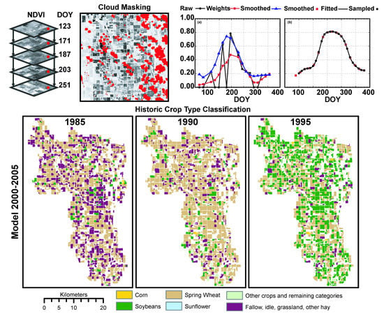
:Long-term temporal and spatial information of crop type supports a wide range of applications including hydrological and climatological studies. In the U.S., yearly crop data layers (CDLs) are available starting in the early 2000s and have been developed using combined field information and sets of temporal imagery from multiple sensors. Development of long-term crop-type layers similar to CDLs is restricted by reduced accessibility to imagery and the necessary auxiliary datasets. In this study, a procedure to generate a historical crop type was developed and evaluated. Time series of Normalized Difference Vegetation Index (NDVI) datasets from Landsat 5 TM sensor for the Lower Bear Creek watershed were collected and processed. Object-based pseudo phenology curves, represented by the NDVI time series, were generated using noise filtering and dimensionality standardization procedures for the years 1985, 1990, 1995, 2000, and 2005. Classifiers were developed and evaluated using random-forest machine learning algorithms and CDL datasets as the reference. Increased generalization performance was obtained when the model was developed using multi-year datasets. This can be attributed to improved crop type representation during the training phase coupled with characterization of yearly variations due to natural (weather) and anthropogenic factors (farming management). Source of uncertainties were the presence of multiple crops within objects, phenological similarities between soybean and corn/maize, and the accuracy of CDL itself. The proposed procedure supports the development of historic crop types for long-term studies at the field scale in agricultural watersheds.
1. Introduction
Datasets on crop type classification and its distribution in space and time support a wide range of direct applications and can be incorporated into a variety of environmental and hydrologic models. The latter allow us to assess the impact of agriculture on the environment, and conversely, the impact of the environment on agriculture [1,2]. These datasets support government agencies, private sector organizations, scientists, educators, and others seeking an improved understanding of cropland spatiotemporal variations and make informed decisions on farming and conservation practices [2,3]. Applications include, but are not limited to, crop yield estimation and prediction [1], natural hazard (e.g., floods and droughts) impact assessment on agricultural commodities [4,5,6], and nonpoint source pollution quantification and mitigation [5,6]. For the latter, hydrological watershed models, in particular the annualized agricultural non-point source (AnnAGNPS) [7,8] and the Soil and Water Assessment Tool (SWAT) [9,10], rely heavily on spatiotemporal crop type information to characterize agricultural watershed and best represent existing conditions of land use and farming practices.
In the U.S., the cropland data layer (CDL) product generated by the U.S. Department of Agriculture (USDA) National Agricultural Statistics Service (NASS) provides a valuable database of crop classification and distribution for the conterminous U.S. [11]. This dataset is heavily used in a multitude of disciplines, applications, and models [12,13,14,15]. The CDL is generated annually by integrating multiple imagery sources such as Landsat products, Moderate Resolution Imaging Spectroradiometer (MODIS), and Resourcesat-1 Advanced Wide Field Sensor (AWiFS) with the objective of maximizing the temporal resolution to capture key phenological stages [16,17]. In addition, imagery is combined with auxiliary datasets such as digital elevation models (DEMs), the U.S. Geological Survey-National Land Cover Dataset (NLCD), and the USDA-Farm Service Agency (FSA)-Common Land Unit (CLU).
Despite the importance of CDL datasets in providing crop-type land cover to hydrological studies and many other disciplines, there are limiting factors for their utilization in long-term investigations. The latter include long term watershed modeling and climatic analysis impact assessment that require at least 30 years of data. CDL datasets available for the contiguous U.S. vary per state, with the most agricultural intense states being covered from 2006 to the present [2]. Development of long-term crop-type layers similar to CDL is restricted by reduced accessibility to satellite imagery (smaller number of missions in earlier years) and the necessary auxiliary datasets. Moreover, the FSA-CLU dataset, which is essential to CDL’s development and accuracy assessment, is considered to contain confidential information and is not made publicly available [16]. The issue is more pronounced in many other countries around the world, which hinders the development of detailed hydrological studies and models for even short-term studies in those areas.
Development of CDL-like datasets relies on the proper estimation of farming practices and crop growth dynamics. Crop dynamics are estimated by using stacked time series of remotely-sensed vegetation indices serving as temporal signatures. Classification is performed by integrating temporal signatures with auxiliary information on crop planting/harvest schedules and sequential crop development phases; assumed to be unique to the individual crop type. Temporal resolution is of vital importance in order to capture the subtle differences in plant growth over time, and subsequently improve the recognition and distinction of different crop types.
Multiple studies have investigated high temporal resolution sensors such as the Moderate Resolution Imaging Spectroradiometer (MODIS) and Advanced Very High Resolution Radiometer (AVHRR) for regional and global scales [18,19,20,21]. Notwithstanding, these studies have addressed the temporal resolution needed for capturing crop growth dynamics at regional or global scales, but these sensors do not offer the necessary spatial resolution for the parcel/field scale. Other studies have investigated methodologies to fuse high temporal resolution (MODIS) with higher spatial resolution (Landsat) [22] or even optical with radar systems (Sentinel) [23] to improve crop type mapping at moderate resolution. However, these studies were based on newer systems (MODIS and Sentinel missions) hindering their utilization specifically for long-term studies. A recent study has investigated the application of the CDL algorithm for historical crop-type classification using Landsat 5TM and 7ETM+, but using the same auxiliary layers as predictors such as the U.S. Geological Survey’s (USGS) National Elevation Datasets (NED), NLCD, and CLU [24]. Though deriving reliable phenology curves solely from remotely sensed products is limited by the presence of data gaps in key important stages of crop development [22], reliance on moderate resolution systems prior to the 2000s such as Landsat 4 and 5 for historical crop-type classification is challenging due to the sensor’s temporal resolution and availability of cloud-free datasets. Attempts to overcome these challenges of incomplete and/or noisy proxy-phenology curves have been investigated using data processing techniques and/or robust classifiers. Data processing techniques such as filtering procedures (de-noising), function fitting (gap filling) [25], and phenological metrics [26,27] have been used to transform the raw proxy-phenology curves to obtain their main properties. Robust classifiers that have been investigated were in the form of non-parametric algorithms [28,29] and include decision trees [26,27,29], artificial neural networks [30], support vector machines [26,27,31], and random forests [26,27,32].
The commonality between these studies is their focus on developing detailed and accurate methodologies for crop type mapping for recent years (2000 to the present). Limited studies were found addressing historical crop type classification at the field scale based solely on remote sensing products. In this manuscript, we developed and evaluated a field scale crop type classification methodology that relies on limited remote sensing datasets (i.e., Landsat products) without requiring any auxiliary data. Limited temporal resolution is addressed by an integrated data processing and filtering method with robust machine learning algorithms. Hence, this methodology could readily be applied in many parts of the world as well as in the U.S. to complement (i.e., 1985–2013) the more recent timeframe covered by CDLs (i.e., 2006–2019). This could provide a historical distribution of cropland for a better understanding of long-term trends in agricultural commodities, yield and variations and their relation with climate change and other long term anthropogenic and natural controlling variables.
2. Materials and Methods
2.1. Study Site
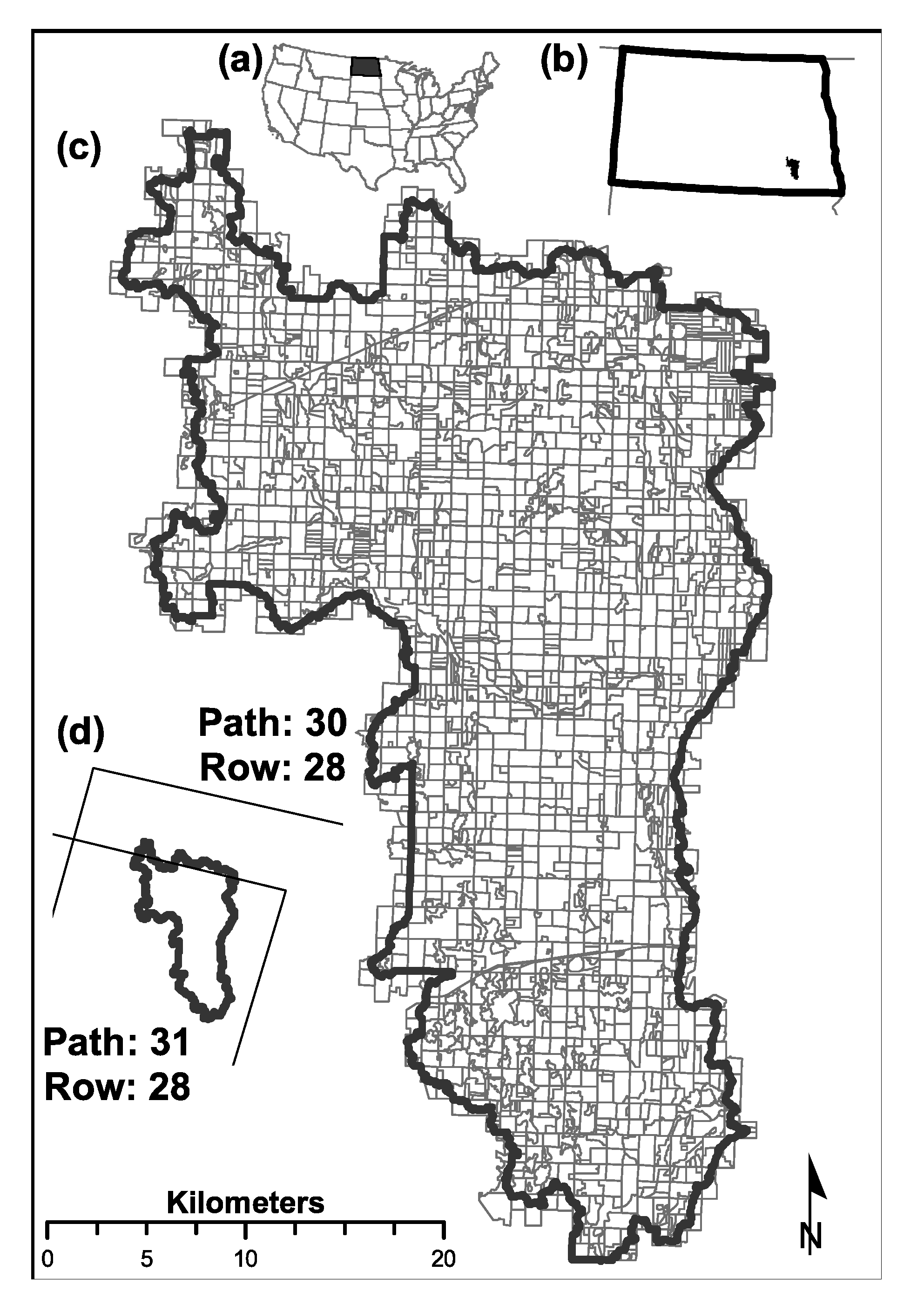
The Lower Bear Creek watershed with an area of 93,833 hectares is located in the southeastern corner of the State of North Dakota, USA (Figure 1). It is characterized by low relief (396 to 894 m a.m.s.l.) and land use/land cover predominantly of agriculture in the form of row crops and grazing fields (> 90%). According to the USDA cropland data layers, in 1998, the main composition land use/land cover was 32% fallow, idle, grass, or pasture, and 60% row crops. The main row crops in 1998 were corn/maize (10%), soybeans (11%), and spring wheat (22%). In 2005, these percentages changed to 14%, 31%, and 16% for corn/maize, soybeans, and spring wheat, respectively. Crop conversion changes aligned well with the national trends of conversion of traditional crops into soybeans and corn/maize. In North Dakota, typical planting and harvesting dates for corn/maize are 2–28 May and 8 October–19 November, for soybean 14 May–3 Jun3 and 24 September–21 October, and for spring wheat 24 April–25 May and 8 August–13 September [33].
2.2. Imagery Acquisition and Processing
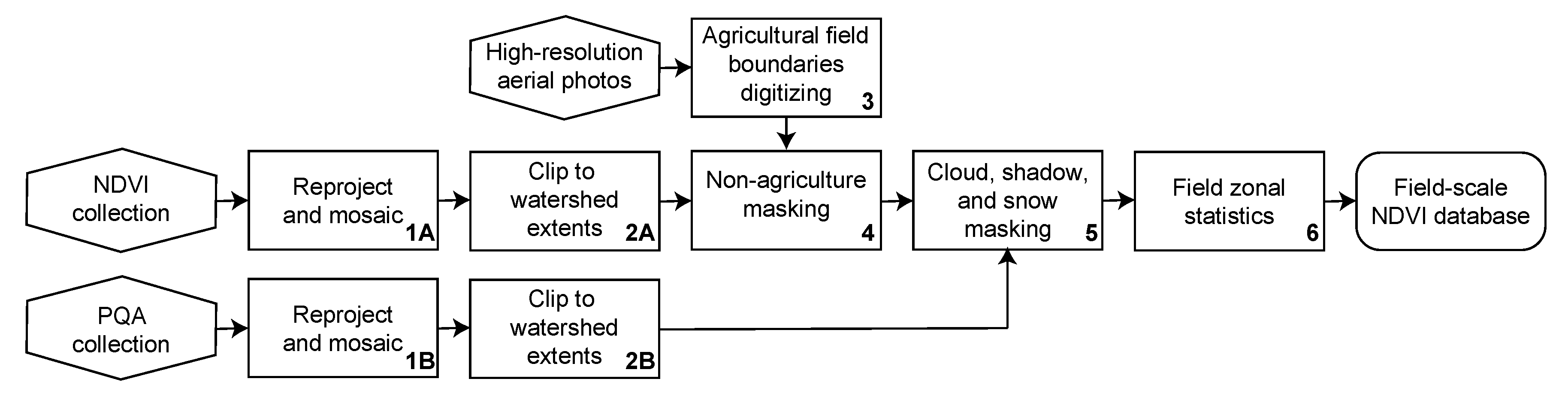
Normalized difference vegetation index (NDVI) and pixel quality metadata (PQA) images were downloaded from the U.S. Geological Survey (USGS)—Earth Resource Observation and Science (EROS)—EROS Science Processing Architecture (ESPA) website [34,35]. All images in the years 1985, 1990, 1995, 2000, and 2005 were downloaded (Table 1). Only images from the Landsat 5TM collection were used because this mission covered all five years considered. The product Landsat surface reflectance-derived spectral indices (NDVI) was chosen to reduce pre-processing steps such as atmospheric correction and spectral index computation [35]. The study site is covered by two Landsat paths (Figure 1d). Both NDVI and PQA images were re-projected (Figure 2, box 1) and clipped to the watershed extents (Figure 2, box 2).
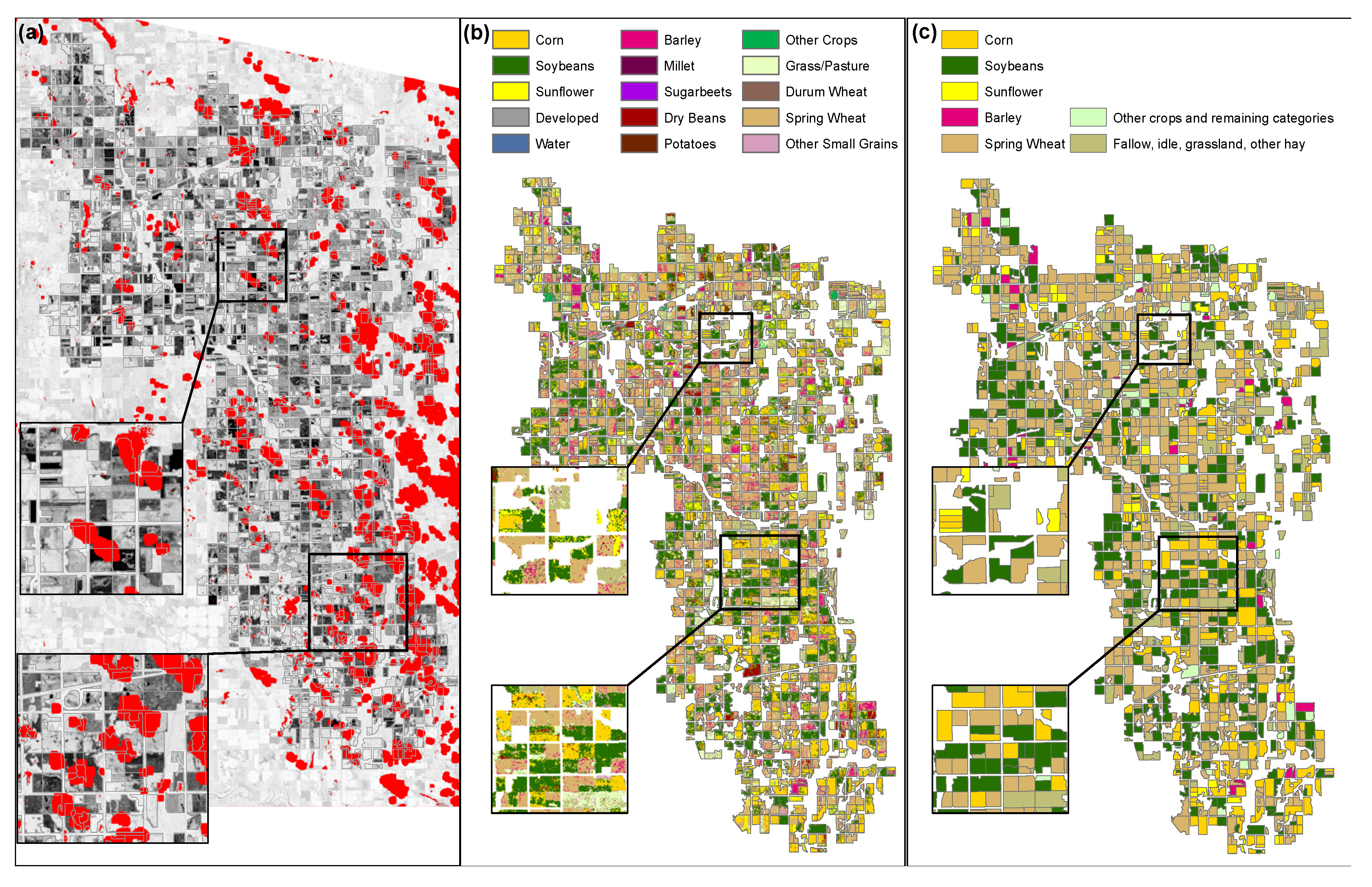
Parcel boundaries were digitized based on high-resolution aerial photographs and labeled as agriculture or non-agriculture, based on the visual inspection of aerial photographs and supporting auxiliary data such as CDL datasets for 2000 and 2005, road centerlines, and NLCD (Figure 2, box 3). Out of 2757 parcels, 1755 were identified as croplands (Figure 1c). Cropland fields were used to generate a non-agriculture mask imagery that was subsequently applied to all NDVI images (Figure 2, box 4). Similarly, a set of masks were developed to filter out the potential influence of clouds, cloud shadows, and snow/ice to the NDVI values using the flags encoded in the PQA images [36,37] and generated by the CFMask algorithm [35] (Figure 2, box 5 and Figure 3a).
Individual images of masked NDVI for cropland and cloud/snow were stacked into five files (one for each year considered). The final NDVI time series images contained a varying number of bands, each representing a day-of-year (DOY). Custom GIS zonal statistics algorithms were developed to calculate the average NDVI value for each DOY (each band) and each field (each image object). A modified zonal statistic algorithm was developed and employed to consider only valid pixels based on previously developed masks (Figure 3a) and to report an average, if a minimum number of five or more valid pixels was found. This information was recorded in a tabular format of one field per row and the sequence of NDVI average values in columns (Figure 2, box 6).
Reference datasets for 2000 and 2005 were derived from the respective CDLs. The raw CDL raster grid layers contained noise (Figure 3b) and were processed through another custom-made zonal statistic algorithm. Common zonal statistics tools found in off-the-shelf GIS software packages calculate the results using all pixels and report only the class number with the majority value found. The algorithm employed recorded the frequency information of all classes found in each parcel, rather than only the most abundant one (Figure 3c). The dominant crop-type for each field was added to the NDVI temporal sequence database generated previously.
2.3. Noise Filtering and Dimensionality Standardization
Clouds, cloud shadows, snow, and ice prevent satellite sensors from directly measuring vegetation growth by obscuring and contaminating areas of interest. Removing cloudy pixels creates troughs (instances of zero growth) in the growth curve that misrepresent the natural vegetation development cycle. Furthermore, the pixel quality assurance band used to mask out images is not perfect. Cloudy or shadowed pixels may persist even after masking with the PQA image. In order to best capture a reliable phenology curve from the aggregated data, noise in the phenology curve must be removed to address the substantial variability inherent to our dataset.
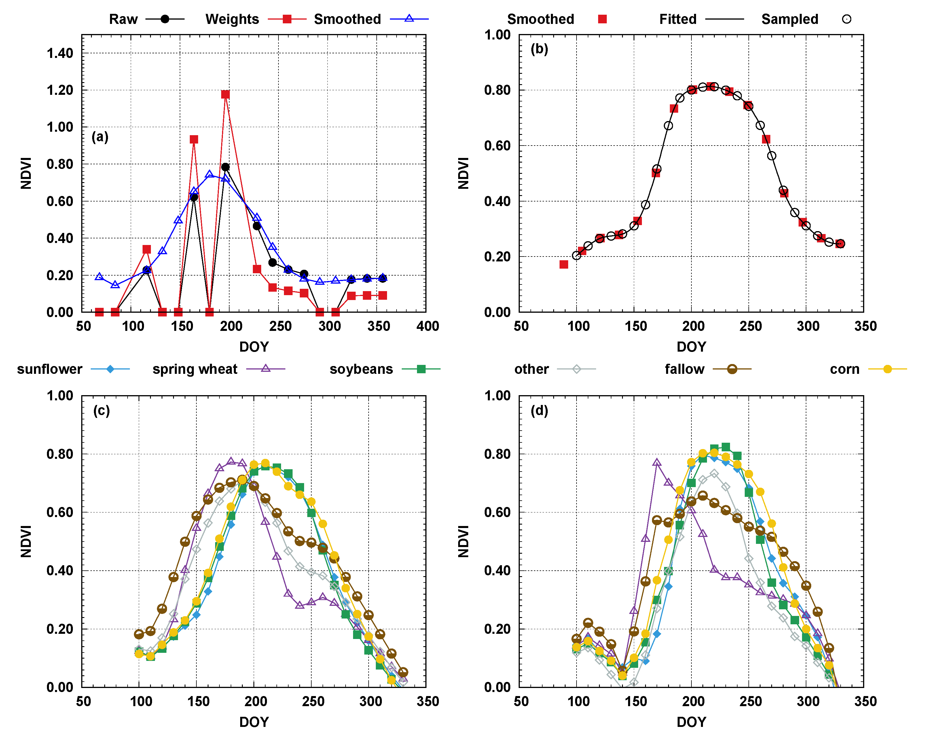
The procedure adopted was the weighted windowed linear regression [38]. Weighted windowed linear regression attempts to address variability by smoothing phenology curves to remove noise. A weight is assigned to each day of the year based on whether the point is a peak point, upward sloping, downward sloping, or a valley point where a peak point receives the highest weight and a valley point receives the lowest weight. A moving window is then used to successively fit a linear equation to each point in the field’s weighted phenology curve. The resulting coefficients are used to calculate a series of weighted NDVI values for each day of year, which are then averaged where peak values are weighted heavier than valleys. The resulting product is a smoothed phenology curve where the growth obscured previously by gaps is restored (Figure 4a). This procedure was applied to all fields and all five years.
Although the smoothed curves are a better representation of field conditions in time, the curve’s dimensionality varied per year and even per fields within the same year. Fields were described by different DOYs and varying number of samples. This was due to differences in the DOY when images were acquired (see Table 1) and potential gaps were present in one field, but not in another. This was addressed through the function fitting approach to existing points using a piecewise cubic polynomial method [39] implemented in the Scientific Computing library of the Python programming language [40,41]. The advantage of this method is the generation of a smooth curve that goes through the observed points. Once the coefficients are determined, the fitted equation can then be used to estimate values at set time intervals. Values were estimated for every 10 days from DOY 100 to DOY 330 (Figure 4b), assuring all curves (all fields and years) contained the same number of points; a requirement for machine learning algorithms. Using the CDL information assigned to each field, averaged curves for prevailing crop types were developed for 2000 (Figure 4c) and 2005 (Figure 4d).
2.4. Models Development and Evaluation
The development/utilization of robust classification algorithms for crop-type classification has relied on machine learning algorithms (non-parametric) [28]. These algorithms are designed to address complex problems without being explicitly programmed to do so, but rather to derive solutions from recursive and iterative analysis of candidate solutions based on a user-provided training dataset [42]. Non-parametric algorithms for time-series analysis have significant advantages. These algorithms have been demonstrated to be distribution independent, work well with missing and/or noise data, have a higher accuracy than standard remote sensing classifiers, and are considered robust (capable of generalization). Multiple machine learning algorithms were evaluated using the WEKA Machine Learning Software package [43] with the random forest classifier [44] selected due to its higher accuracy over the artificial neural network, decision trees, and support vector machine. Random forest is described as an ensemble data mining/classification algorithm because it evolves and evaluates a set of independent tree-based classifiers concurrently. During the development of candidate solutions, the algorithm relies on bootstrapping techniques for improved conversion by assuring diversity [32]. For classification problems, assignment of an instance to class is based on predictions from all trees (majority voting). The limitations of this approach is that the individual classification trees are not available to the user and it can be computationally intense. Conversely, this method has the advantages of being able to quantify the importance of each input variable, it yields higher accuracy than traditional decision trees, and can generate accurate robust classifiers [42].
In this study, each crop field (image object) for a specific year corresponded to an instance. Each instance was described by 23 processed NDVI values for pre-determined DOYs between DOY 100–330 (representing growing season) at a 10-day time step (input variable) plus label information, when available (for 2000 and 2005 only). A total of three models were developed using NDVI images and CDL from 2000, 2005, and combined 2000–2005. For models developed using a single year, training was performed using cross-validation with 10 folds and testing using the other year. For the combined 2000–2005 datasets, the dataset was randomly divided into 66% for training and 33% for testing. During the development, the random forest algorithm proposed by [44] and implemented in the WEKA software package [43] was used with the following controlling parameters: bag size of 100%, minimum numeric class variance proportion of train variance for split of 0.001, minimum number of variables per leaf of 1, and maximum number of iterations of 1000. Models were assessed using standard statistics of overall accuracy and kappa coefficient of agreement [45] derived from the confusion matrix.
3. Results
3.1. Pseudo Crop Phenology Curves
Analysis of the average NDVI curves for each class and each time period (Figure 4c,d) indicates patterns within crops (same crop different time period) and between crops (different crops). There are phenological similarities between corn, soybeans, and sunflower crops. These temporal signature similarities could restrain the classifier’s performance of discerning between them. The similarities were more pronounced in 2000 (Figure 4c) than in 2005 (Figure 4d), signifying yearly variations. Conversely, spring wheat, other crops, and fallow/pasture/grassland presented more distinguished temporal signatures with earlier development, followed by varying harvest/declining stages.
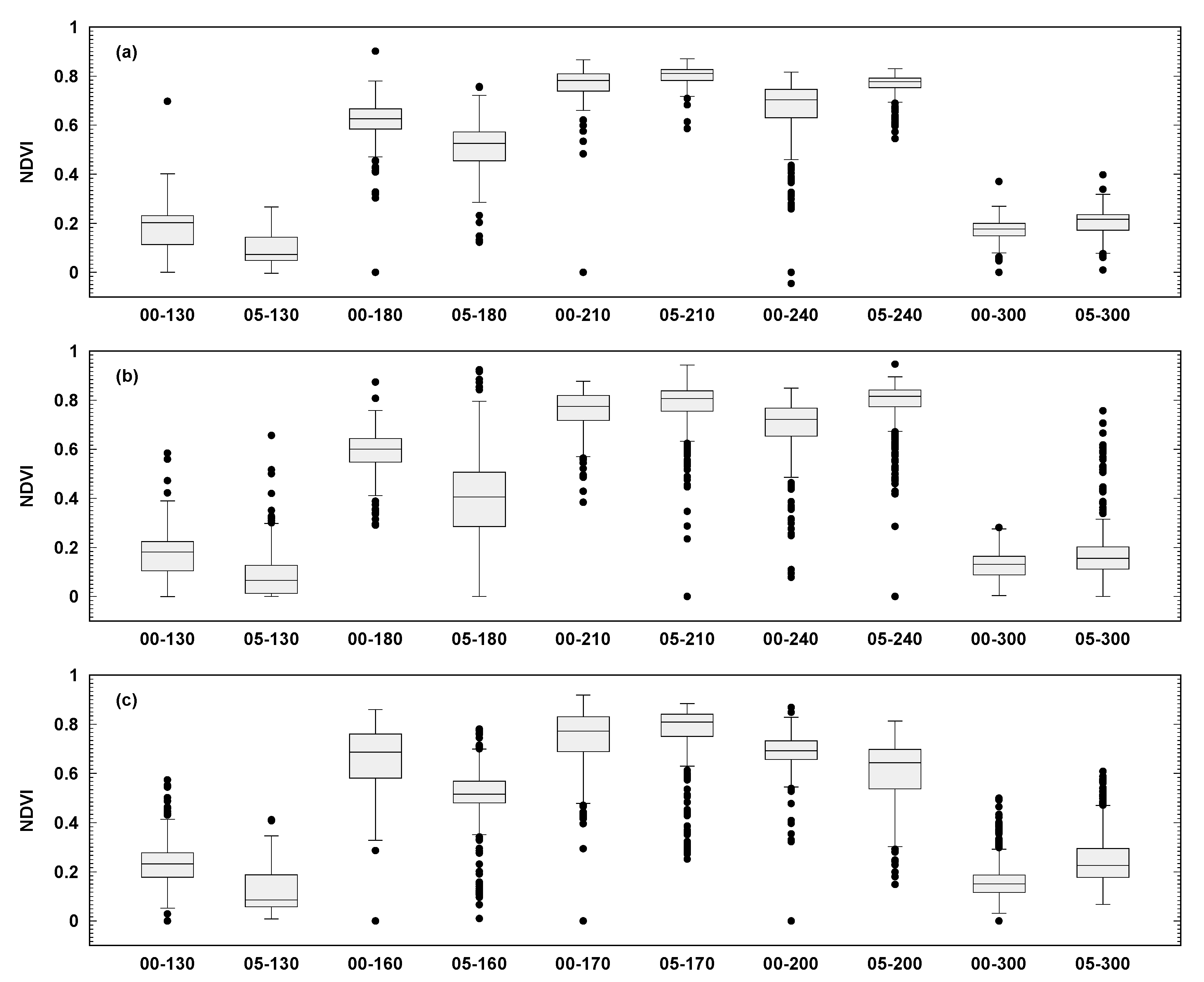
Distributions of the NDVI-based phenology curves for the three dominant crops (corn/maize, soybeans, and spring wheat) in 2000 and 2005 at five time periods during the crop calendar revealed inter-field and inter-year variations (Figure 5). Inter-field analysis through comparisons of NDVI distributions for a particular crop at a particular year provided an indication of noise in the dataset. For instance, the NDVI distribution values for spring wheat in 2000 at DOY160 (June) and DOY200 (July) yielded standard deviation values of 0.12 and 0.06, respectively (Figure 6c). Crop inter-year variability is influenced by how natural changes influence crop biomass over the growing period and crop conversion patterns. Differences in NDVI distribution values for the same crop growth period between 2000 and 2005 indicate an external factor affecting the entire region. For example, soybeans values for DOY 210 between 2000 and 2005 indicated that the crops reached maturity in the entire region (see DOY210 in Figure 5b), as demonstrated by the standard deviation values for both distributions of 0.08 and means of 0.76 and of 0.78 for 2000 and 2005, respectively. Conversely, in the same analysis, for DOY 180, there was a discrepancy between the two distributions for the entire region with mean and standard deviation values of 0.59 and 0.09 and 0.40 and 0.16 for 2000 and 2005, respectively. This discrepancy signifies region-wide changes potentially from differences in weather patterns between years.
3.2. Models Development and Evaluation
Single year models were comparable (Table 2) and yielded high overall accuracy and kappa coefficient of agreement values for both training and testing (kappa > 0.55 and OA > 0.67). However, despite the model’s overall high performance, a misclassification of corn/maize, soybeans, and sunflower can be noted. This can be attributed to the phenological similarities between these crops (yellow circle, blue diamond, and green square curves in Figure 4c,d).
The 2005 model yielded the highest single year training accuracy values (k = 0.87 and OA = 90.92%), but with the lowest testing accuracy values (k = 0.52 and OA = 67.30%) when evaluated using the 2000 dataset. In the 2005 dataset, only 12 fields were labeled as sunflower and only nine were designated as other crops. This small number of fields was not representative enough during the model development stage and therefore in the model’s evaluation using the 2000 dataset, no fields were assigned to neither sunflower nor other crops. This lack of representation by individual class was addressed by combining both single year datasets of 2000 and 2005 into a single dataset to develop a new combined model (see combined 2000–2005 confusion matrix in Table 2) with improved accuracy values. The 2000–2005 model yielded accuracy statistics of 0.86 and 90% for the kappa and overall accuracy, respectively.
3.3. Model Application
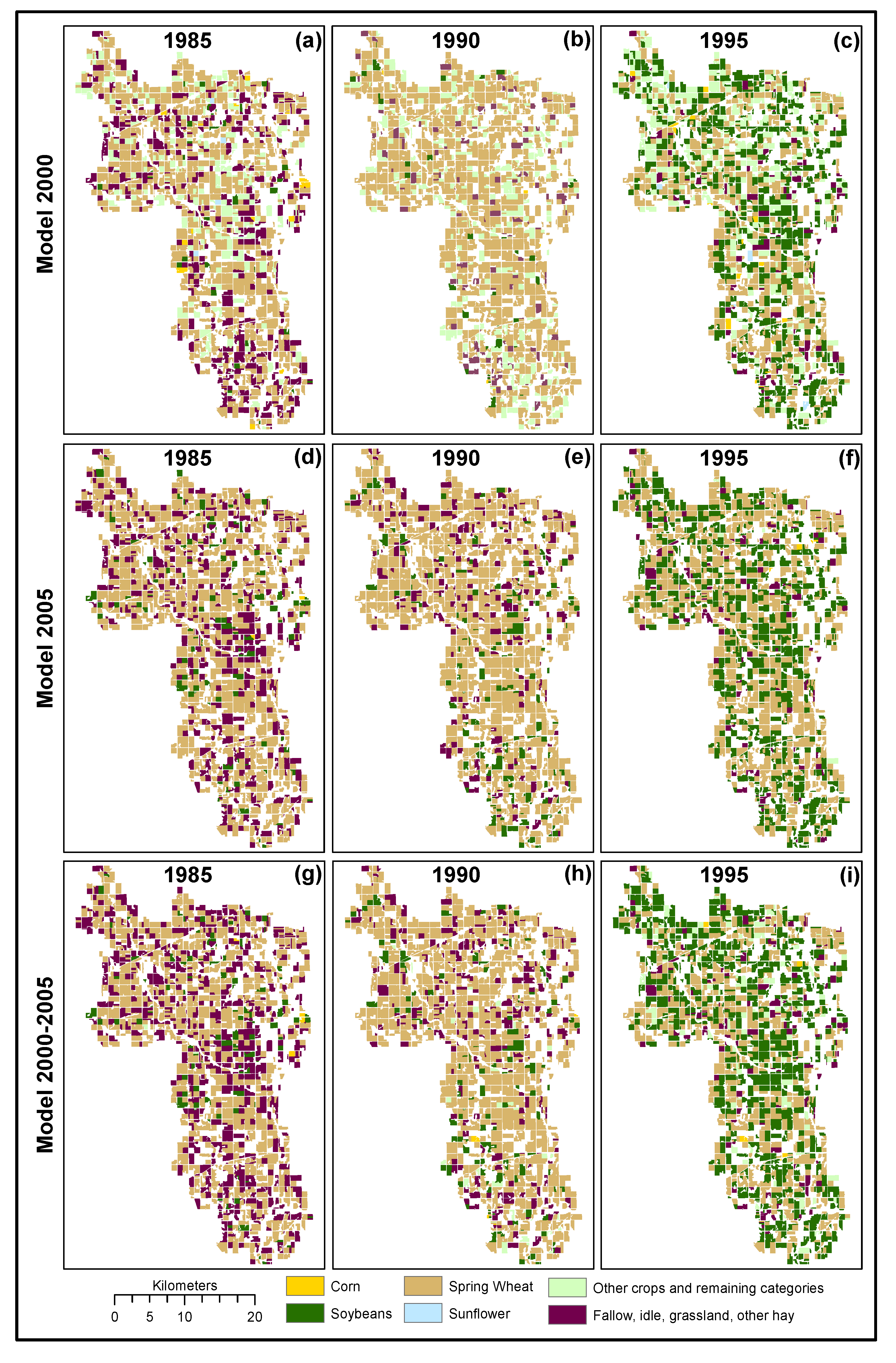
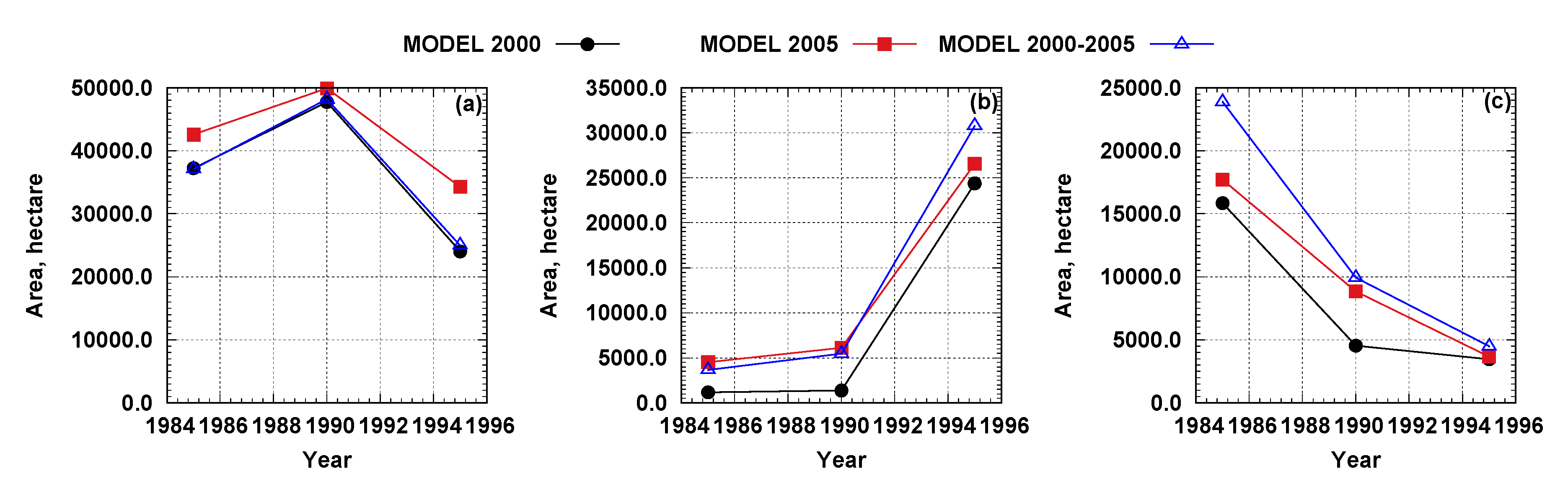
The three models developed, 2000, 2005, and combined 2000–2005 were applied to process the NDVI time series for 1985, 1990, and 1995; years for which CDL datasets are not available (Figure 6). The lack of reference, prevented absolute accuracy assessment and therefore a relative accuracy assessment was performed by comparing the predictions between models. Evaluating the agreement amongst all three models for the predicted correctly planted area for all classes was 68.7%, 75.9%, and 65.46% for 1985, 1990, and 1995, respectively. Slightly higher agreement amongst the three models was observed for 1990. Considering the agreement between the pairs of models, higher agreement was obtained between models 2000–2005 and 2005 for 1985 (88.7%) and 1990 (90.9%) and between models 2000–2005 and 2000 for 1995 (78.7%).
4. Discussion
4.1. Pseudo Crop Phenology Curves
Working in the object domain, rather than in the pixel domain, has advantages. First, working with image objects removes the need for geospatial registration (georectification) between images to assure that individual pixels align spatially (since temporal signatures are generated by stacking multiple scenes). Georectification is a process that is hard to automate, and therefore often relies heavily on manual labor that is time-consuming and can add subjectivity. Using an object-based approach for the temporal analysis of spectral indices provides spatially smoothed NDVI values (field mean), reducing the noise/influence from individual pixel outliers. It increases the availability of data when information from an object is partially compromised (field partially covered by clouds). Additionally, there is significant reduction in the data volume from going from pixel to object scales (from millions of pixels to hundreds of fields). Similar studies have found that working in the object domain rather than in the pixel domain reduces noise and, as result, yields improved accuracy results [27,46]. However, changing from pixel to object is not without its challenges. There is the need to define field boundaries. In this study, this was done by heads-up digitizing using CDL and aerial photographs from one time period, therefore, it is possible that the field boundaries changed over time. Furthermore, a field could contain more than one crop in a particular growing season, causing potential bias in the average NDVI values. This was addressed by changing from simple majority voting (standard GIS zonal statistics operation) to determining the percentage of each crop in each field, and then using only fields with a percent majority greater than 50% (custom-developed zonal statistic).
The final processed phenology curve used in the models did not contain gaps. These curves are generated by two procedures: noise filtering (weighted windowed linear regression) and dimensionality standardization (piecewise cubic polynomial). However, these datasets are not immune to noise. Inter-field variations could be potentially attributed to gaps in the dataset (clouds) incorrectly filled by subsequent steps, inconsistencies in the CDL layer used as the reference, or contaminated pixels (cloud shadows) affecting the individual time period. This uncertainty is often addressed with increased temporal resolution, but remains a challenge when the objective is to classify historic datasets where temporal resolution is limited.
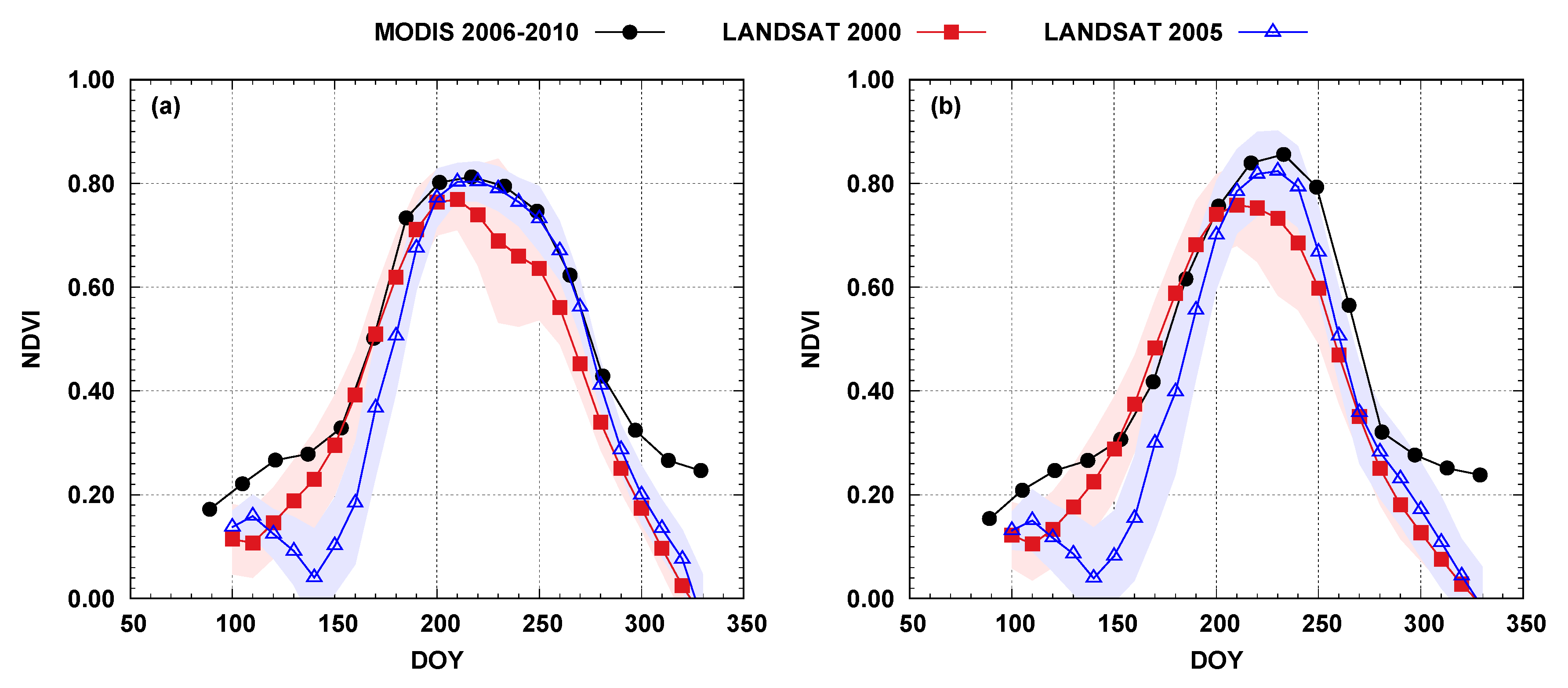
Averaged curves generated for corn and soybeans were compared with state-wide five-year averaged curves generated using MODIS (Figure 7) [47]. For both crops in 2000, this comparison demonstrated a standard development stage, but with a shorter peak, followed by an earlier decline. The shaded area in Figure 7 describes the variance represented by one standard deviation. It can be observed a higher variance for 2000 between DOY 210 and DOY 260. The curves generated in 2005, despite a slightly late start, matched the state-wide averages. The late start can be attributed to abnormally dry weather between April 26, 2005 to May 31, 2005 [48] followed by high rainfall amounts in May/June. The comparisons of the developed with published curves generated using different procedures yielded confidence in the method proposed as they aligned well with findings from other studies, while at the same time, signified challenges inherent in multi-year crop phenological development modeling (influence of natural and anthropogenic factors).
4.2. Models Development and Evaluation
The main source of single year model misclassifications was due to similarities in the NDVI-based phenology curves. These similarities in the NDVI curves, representing different crops, can be potentially attributed to parallel farming operation schedules coupled with comparable crop biomass changes over the growing cycle. Challenges in signal separability between the NDVI-based phenology curves of major row crops have also been reported in other studies [26,32,47]. These similarities in temporal signatures pose a challenge to classifier algorithms, although in this study, it was more pronounced in the 2000 than in the 2005 dataset.
Annual variations also influenced the model’s robustness, represented by the ability to generalize when presented with datasets not used during the training stage. Single year developed models were vulnerable to anthropogenic and natural induced watershed-wide changes. Anthropogenic factors such as crop conversion influenced how well a particular crop type class is represented during the model development (training stage). Based on reference data generated from CDLs from 2000 to 2005, an increase in corn/maize (from 182 to 220 fields) and soybean (from 292 to 676 fields) was observed in this watershed, but a decrease in spring wheat (from 534 to 377 fields) and sunflower (from 47 to 12 fields). This regional trend is consistent with national crop conversion moves toward corn/maize and soybean rotations [49,50]. Natural factors are simply due to climatic variations [48]. Developing models based on multiyear datasets has addressed uncertainties by annual variations. Results from the 2000–2005 model are in agreement with similar studies in China [27], Brazil [31], and Kansas, USA [26], despite the fact these studies used a higher temporal resolution either by using MODIS or combining different platforms.
It is important to acknowledge the accuracy of CDL layers calculated at the pixel scale. For the 2000 CDL, an overall accuracy of 88.66 and of 69.53 and kappa coefficient of 0.86 and 0.65 were reported for path 30–row 28 and path 31–row 28, respectively. Similarly, for the 2005 CDL, overall, the accuracy values of 74.01 and 69.53 and kappa coefficient of agreement of 0.68 and 0.65 were obtained [51]. These accuracy values suggest a potential source of uncertainty influencing the model development and were documented in similar studies [26].
4.3. Model Application
The lack of historic reference data prevented the absolute accuracy assessment of crop type generated for 1985, 1990, and 1995. However, relative comparisons between the different model’s predictions demonstrated agreement in the dominant crop area estimation and between pairs of models. The agreement between models can also be observed in the crop-type conversion trend (Figure 8). Spatial models (Figure 6) in conjunction with temporal models (Figure 8) support the development of input databases capturing the dominant crop-conversion trends, which is important information for long-term hydrological/climatic studies designed to characterize existing conditions over time.
5. Conclusions
Long-term hydrological and/or climatological modeling studies of agriculture watersheds depend on reliable crop-specific land cover information. This study proposed and evaluated methods for deriving such datasets solely based on the time series of satellite imagery through integrating data processing methods (filtering and data gap filling) with non-parametric classifying algorithms (random forest algorithm). Uncertainties in mis-registration between images was addressed by working in the object domain, represented by farm fields, rather than the pixel domain. Additional advantages of working in the object domain versus the pixel domain include the possibility of increasing the temporal resolution by being able to use objects that are partially contaminated (either clouds or no-data pixels), the significant reduction in data volume (from millions to thousands), and the generation of smoothed datasets (field averaged). In contrast, field boundaries were assumed to be static over time. In a small number of fields, the cultivation of more than one crop type in a single season (field is split into two or three crops) was observed. This was addressed by developing custom zonal statistical algorithms to consider only fields where a single crop-type covered more than 50% of the field. Future studies could investigate the use of image segmentation algorithms as possible alternatives to develop dynamic image objects (field boundaries changing from year to year).
Predictive model development based on single year datasets (NDVI and CDL) yielded adequate overall accuracy results for both the training and testing datasets. The main sources of uncertainties in the model development were phenological similarities between the crop-type and representativeness of crop type within the training datasets. The later uncertainty was addressed through the utilization of the multi-year training dataset. This approach has the advantage of increasing crop type representation during the training phase and capturing potential yearly variations due to natural and anthropogenic factors.
The integration of machine learning algorithms, enhanced signal filtering, and dimensionality standardization through function fitting with remotely sensed time series of spectral indices to develop historic crop data layers at the field scale is a feasible alternative. This approach has the potential to temporally extend CDL coverage in the USA, and therefore support long-term hydrological/climatological modeling of agriculture watersheds. Accurate crop-type characterization influences how farming practices are modeled in time and space and therefore how non-point source pollutants are produced, transported, and deposited; thus, supporting the development of effective mitigation strategies.
Author Contributions
Conceptualization, H.G.M. and R.E.; Methodology, H.G.M.; Software, H.G.M. and W.P.; Validation, H.G.M. and W.P.; Formal analysis, H.G.M. and W.P.; Writing—original draft preparation, H.G.M., W.P., and R.E.; Writing—review and editing, H.G.M. and R.E.; Supervision, H.G.M. and R.E.; Project administration, H.G.M.; Funding acquisition, H.G.M. and R.E. All authors have read and agreed to the published version of the manuscript.
Funding
This research was funded by the Non-Land-Grant Colleges of Agriculture (NLGCA) grants program, grant number 1214959, and project accession number 1010585 from the U.S. Department of Agriculture (USDA) National Institute of Food and Agriculture (NIFA).
Acknowledgments
The authors would like to acknowledge Joel Miranda Paniagua and Miranda McBride for their technical support in the dataset processing.
Conflicts of Interest
The authors declare no conflicts of interest.
References
- Gilmanov, T.G.; Wylie, B.K.; Tieszenb, L.L.; Meyers, T.P.; Barond, V.S.; Bernacchi, C.J.; Billesbach, D.P.; Burba, G.G.; Fischer, M.L.; Glenni, A.J.; et al. CO2 uptake and ecophysiological parameters of the grain crops of midcontinent North America: Estimates from flux tower measurements. Agric. Ecosyst. Environ. 2013, 164, 162–175. [Google Scholar] [CrossRef] [Green Version]
- Howard, D.M.; Wylie, B.K. Annual crop type classification of the US great plains for 2000 to 2011. Photogramm. Eng. Remote Sens. 2014, 80, 537–549. [Google Scholar] [CrossRef]
- Boryan, C.; Yang, Z.; Mueller, R.; Craig, M. Monitoring US agriculture: the US Department of Agriculture, National Agricultural Statistics Service, Cropland Data Layer Program. Geocarto Int. 2011, 26, 341–358. [Google Scholar] [CrossRef]
- Song, X.; Potapov, P.V.; Krylov, A.; King, L.; Bella, C.M.D.; Hudson, A.; Khan, A.; Adusei, B.; Stehman, S.V.; Hansen, M.C. National-scale soybean mapping and area estimation in the United States using medium resolution satellite imagery and field survey. Remote Sens. Environ. 2017, 190, 383–395. [Google Scholar] [CrossRef]
- Otkin, J.A.; Anderson, M.C.; Hain, C.; Svoboda, M.; Johnson, D.; Mueller, R.; Tadesse, T.; Wardlow, B.; Brown, J. Assessing the evolution of soil moisture and vegetation conditions during the 2012 United States flash drought. Agric. For. Meteorol. 2016, 218, 230–242. [Google Scholar] [CrossRef] [Green Version]
- Momm, H.G.; Porter, W.S.; Yasarer, L.; ElKadiri, R.; Bingner, R.L.; Aber, J. Crop Conversion Impacts on Runoff and Sediment Loads in the Upper Sunflower River Watershed. Agric. Water Manag. 2019, 217, 399–412. [Google Scholar] [CrossRef]
- Zema, D.A.; Bingner, R.L.; Denisi, P.; Govers, G.; Licciardello, F.; Zimbone, S.M. Evaluation of runoff, peak flow and sediment yield for events simulated by the AnnAGNPS model in a Belgian agricultural watershed. Land Degrad. Dev. 2012, 23, 205–215. [Google Scholar] [CrossRef]
- Bisantino, T.; Bingner, R.L.; Chouaib, W.; Gentile, F.; Liuzzi, G.T. Estimation of runoff, peak discharge and sediment load at the event scale in a medium-size Mediterranean watershed using the AnnAGNPS model. Land Degrad. Dev. 2013, 26, 340–355. [Google Scholar] [CrossRef]
- Srinivasan, R.; Zhang, X.; Arnold, J. SWAT Ungauged: Hydrological Budget and Crop Yield Predictions in the Upper Mississippi River Basin. Trans. ASABE 2010, 53, 1533–1546. [Google Scholar] [CrossRef]
- Arnold, J.G.; Williams, J.R.; Maidment, D.R. Continuous-time water and sediment-routing model for large basins. J. Hydraulic Eng. 1995, 121, 171–183. [Google Scholar] [CrossRef]
- Johnson, D.M.; Mueller, R. The 2009 Cropland Data Layer. Photogramm. Eng. Remote Sens. 2010, 1201–1205. [Google Scholar]
- Alemu, W.G.; Henebry, G.M.; Melesse, A.M. Land Surface Phenologies and Seasonalities in the US Prairie Pothole Region Coupling AMSR Passive Microwave Data with the USDA Cropland Data Layer. Remote Sens. 2019, 11, 2550. [Google Scholar] [CrossRef] [Green Version]
- McNider, R.T.; Handyside, C.; Doty, K.; Ellenburg, W.L.; Cruise, J.F.; Christy, J.R.; Moss, D.; Sharda, V.; Hoogenboom, G.; Caldwell, P. An integrated crop and hydrologic modeling system to estimate hydrologic impacts of crop irrigation demands. Environ. Model. Softw. 2015, 72, 341–355. [Google Scholar] [CrossRef] [Green Version]
- Stern, A.J.; Doraiswamy, P.; Akhmedov, B. Crop rotation changes in Iowa due to ethanol production. In Proceedings of the 2008 IEEE International Geoscience and Remote Sensing Symposium, Boston, MA, USA, 6–11 July 2008. [Google Scholar] [CrossRef]
- Baskaran, L.; Jager, H.I.; Schweizer, P.E.; Srinivasan, R. Progress toward evaluating the sustainability of switchgrass as a bioenergy crop using the SWAT model. Trans. ASABE 2010, 53, 1547–1556. [Google Scholar] [CrossRef]
- Boryan, C.; Yang, Z.; Sandborn, A.; Willis, P.; Haack, B. Operational Agricultural Flood Monitoring With Sentinel-1 Synthetic Aperture Radar. In Proceedings of the 2018 IEEE International Geoscience and Remote Sensing Symposium, Valenca, Spain, 22–27 July 2018. [Google Scholar] [CrossRef]
- Torbick, N.; Huang, X.; Ziniti, B.; Johnson, D.; Masek, J.; Reba, M. Fusion of Moderate Resolution Earth Observations for Operational Crop Type Mapping. Remote Sens. 2018, 10, 1058. [Google Scholar] [CrossRef] [Green Version]
- Gu, Y.; Brown, J.F.; Miura, T.; Leeuwen, W.J.D.; Reed, B.C. Phenological Classification of the United States: A Geographic Framework for Extending Multi-Sensor Time-Series Data. Remote Sens. 2010, 2, 526–544. [Google Scholar] [CrossRef] [Green Version]
- Wardlow, B.D.; Egbert, S.L. Large-area crop mapping using time-series MODIS 250 m NDVI data: An assessment for the U.S. Central Great Plains. Remote Sens. Environ. 2008, 112, 1096–1116. [Google Scholar] [CrossRef]
- Zeng, L.; Wardlow, B.D.; Wang, R.; Shan, J.; Tadesse, T.; Hayes, M.J.; Li, D. A hybrid approach for detecting corn and soybean phenology with time-series MODIS data. Remote Sens. Environ. 2016, 181, 237–250. [Google Scholar] [CrossRef]
- Zhong, L.; Hu, L.; Yu, L.; Gong, P.; Biging, G.S. Automated mapping of soybean and corn using phenology. ISPRS J. Photogramm. Remote Sens. 2016, 119, 151–164. [Google Scholar] [CrossRef] [Green Version]
- Gao, F.; Anderson, M.C.; Zhang, X.; Yang, Z.; Alfieri, J.G.; Kustas, W.P.; Mueller, R.; Johnson, D.M.; Prueger, J.H. Toward mapping crop progress at field scales through fusion of Landsat and MODIS imagery. Remote Sens. Environ. 2017, 188, 9–25. [Google Scholar] [CrossRef] [Green Version]
- Tricht, V.T.; Gobin, A.; Gilliams, S.; Piccard, I. Synergistic Use of Radar Sentinel-1 and Optical Sentinel-2 Imagery for Crop Mapping: A Case Study for Belgium. Remote Sens. 2018, 10, 1642. [Google Scholar] [CrossRef] [Green Version]
- Johnson, M.D. Using the Landsat archive to map crop cover history across the United States. Remote Sens. Environ. 2019, 232, 111286. [Google Scholar] [CrossRef]
- Vorobiova, N.; Cherov, A. Curve fitting of MODIS NDVI time series in the task of early crops identification by satellite images. Procedia Eng. 2017, 201, 184–195. [Google Scholar] [CrossRef]
- Hao, P.; Zhan, Y.; Wand, L.; Niu, Z.; Shakir, M. Feature Selection of Time Series MODIS Data for Early Crop Classification Using Random Forest: A Case Study in Kansas, USA. Remote Sens. 2015, 7, 5347–5369. [Google Scholar] [CrossRef] [Green Version]
- Hao, P.; Wang, P.; Niu, A. Comparison of Hybrid Classifiers for Crop Classification Using Normalized Difference Vegetation Index Time Series: A Case Study for Major Crops in North Xinjiang, China. PLoS ONE 2015, 10, 1–24. [Google Scholar] [CrossRef]
- Gómez, C.; White, J.C.; Wulder, M.A. Optical remotely sensed time series data for land cover classification: A review. ISPRS J. Photogram. Remote Sens. 2016, 116, 55–72. [Google Scholar] [CrossRef] [Green Version]
- Friedl, M.A.; Brodley, C.E.; Sthrhler, A.H. Maximizing Land Cover Classification Accuracies Produced by Decision Trees at Continental to Global Scales. IEEE Trans. Geosci. Remote Sens. 1999, 37, 969–977. [Google Scholar] [CrossRef]
- Atzberger, C.; Rembold, F. Mapping the Spatial Distribution of Winter Crops at Sub-Pixel Level Using AVHRR NDVI Time Series and Neural Nets. Remote Sens. 2013, 5, 1335–1354. [Google Scholar] [CrossRef] [Green Version]
- Abade, N.A.; Júnior, O.A.C.; Guimarães, R.F.; Oliveira, S.N. Comparative Analysis of MODIS Time-Series Classification Using Support Vector Machines and Methods Based upon Distance and Similarity Measures in the Brazilian Cerrado-Caatinga Boundary. Remote Sens. 2015, 7, 12160–12191. [Google Scholar] [CrossRef] [Green Version]
- Tatsumi, K.; Yamashiki, Y.; Torres, M.A.C.; Taipe, C.L.R. Crop classification of upland fields using Random forest of time-series Landsat 7 ETM+ data. Comput. Electron. Agricul. 2015, 115, 171–179. [Google Scholar] [CrossRef]
- USDA-NASS 2. Field Crops Usual Planting and Harvesting Dates, USDA-NASS Agricultural Handbook Number 628. 2010. Available online: https://usda.library.cornell.edu/concern/publications/vm40xr56k?locale=en (accessed on 5 June 2019).
- USGS-EROS-ESPA. Available online: https://espa.cr.usgs.gov (accessed on 15 February 2018).
- Masek, J.G.; Vermote, E.F.; Saleous, N.; Wolfe, R.; Hall, F.G.; Huemmrich, F.; Gao, F.; Kutler, J.; Lim, T.K. A Landsat surface reflectance dataset for North America, 1990-2000. IEEE Geosci. Remote Sens. Lett. 2006, 3, 68–72. [Google Scholar] [CrossRef]
- Zhu, Z.; Woodcock, C.E. Object-based cloud and cloud shadow detection in Landsat imagery. Remote Sens. Environ. 2012, 118, 83–94. [Google Scholar] [CrossRef]
- Earth Resources Observation And Science (EROS) Center. Landsat Quality Assessment ArcGIS Toolbox; U.S. Geological Survey: Reston, VA, USA, 2017. [CrossRef]
- Swets, D.; Reed, B.C.; Rowland, J.; Marko, S.E. A weighted least-squares approach to temporal NDVI smoothing. In Proceedings of the From image to information: 1999 ASPRS Annual Conference, Portland, OR, USA, 17–21 May 1999. [Google Scholar]
- Dierckx, P. Curve and Surface Fitting with Splines; Oxford University Press: Oxford, UK, 1993. [Google Scholar]
- Oliphant, T.E. Python for Scientific Computing. Comput. Sci. Eng. 2007, 9, 10–20. [Google Scholar] [CrossRef] [Green Version]
- Millman, K.J.; Aivazis, M. Python for Scientists and Engineers. Comput. Sci. Eng. 2011, 13, 9–12. [Google Scholar] [CrossRef] [Green Version]
- Mitchell, T.M. Machine Learning; McGraw-Hill: New York, NY, USA, 1997; ISBN 0-07-115467-1. [Google Scholar]
- Witten, I.H.; Frank, E.; Hall, M.A. Data Mining: Practical Machine Learning Tools and Techniques, 4th ed.; Morgan Kaufmann: San Francisco, CA, USA, 2016; pp. 486–500. [Google Scholar]
- Breiman, L. Random forests. Mach. Learn. 2001, 45, 5–32. [Google Scholar] [CrossRef] [Green Version]
- Cohen, J. A coefficient of agreement for nominal scales. Educ. Psychol. Meas. 1960, 20, 37–46. [Google Scholar] [CrossRef]
- Ok, A.O.; Akar, O.; Gungor, O. Evaluation of random forest method for agricultural crop classification. Eur. J. Remote Sens. 2012, 45, 421–432. [Google Scholar] [CrossRef]
- Johnson, D.M. A 5-year Analysis of Crop Phenologies from the United States Heartland. In Proceedings of the 2010 Fall Meeting of American Geophysical Union, San Francisco, CA, USA, 13–17 December 2010. B33C-0413. [Google Scholar]
- United States Draught Monitor. Available online: https://droughtmonitor.unl.edu/Maps/MapArchive.aspx (accessed on 20 June 2019).
- Wallander, S.; Claassen, R.; Nickerson, C. The Ethanol Decade: An Expansion of US Corn Production, 2000–2009. USDA-ERS Economic Information Bulletin; 2011; 79. Available online: https://www.ers.usda.gov/webdocs/publications/44564/6905_eib79.pdf?v=41055 (accessed on 2 June 2019).
- Wright, C.K.; Wimberly, M.C. Recent land use change in the Western Corn Belt threatens grasslands and wetlands. Proc. Natl. Acad. Sci. USA 2013, 110, 4134–4139. [Google Scholar] [CrossRef] [Green Version]
- USDA-NASS. Available online: https://www.nass.usda.gov/Research_and_Science/Cropland/metadata/meta.php (accessed on 15 June 2019).
Figure 1.
The Lower Bear Creek watershed is located in the northern part of the U.S. (a) at the southeast corner of the state of North Dakota (b). Field boundaries were digitized using high-resolution aerial photographs combined with the U.S. Department of Agriculture Crop Data Layer datasets (c). The watershed is covered by two Landsat TM5 scene footprints (d).

Figure 2.
Simplified workflow of field-scale Normalized Difference Vegetation Index (NDVI) database development.
Figure 2.
Simplified workflow of field-scale Normalized Difference Vegetation Index (NDVI) database development.

Figure 3.
Development of input and reference datasets for individual agricultural fields. Red patches represent clouds used to mask/remove contaminate pixels during the field spatial aggregation of NDVI pixel values (a). The raw crop data layer (CDL) dataset (b) was processed to determine the majority crop type for each field based on the pixel-field zonal statistics (c). This operation was performed for the 2000 (shown) and 2005 datasets.

Figure 4.
Filtering of the raw NDVI temporal sequences using a weighted least-squares method [38] (a). The filtered curves were re-sampled to address data dimensionality differences at constant 10-day intervals (b). Average resampled curves for 2000 (c) and 2005 (d) for the six classes considered: (1) sunflower, (2) spring wheat, (3) soybeans, (4) corn/maize, (5) other crops, and (6) fallow, idle, grassland, and all other hay.

Figure 5.
Boxplot of five selected time periods in the phenological cycle for corn/maize (a), soybeans (b), and spring wheat (c). In the x-axis, the first number represents the year (00 = 2000 and 05 = 2005) and second number day of the year.
Figure 5.
Boxplot of five selected time periods in the phenological cycle for corn/maize (a), soybeans (b), and spring wheat (c). In the x-axis, the first number represents the year (00 = 2000 and 05 = 2005) and second number day of the year.

Figure 6.
Crop-type predictions at the field-scale generated using machine learning models developed using Landsat NDVI time series and crop data layers of 2000 (a–c), 2005 (d–f), and combined 2000–2005 (g–i).
Figure 6.
Crop-type predictions at the field-scale generated using machine learning models developed using Landsat NDVI time series and crop data layers of 2000 (a–c), 2005 (d–f), and combined 2000–2005 (g–i).

Figure 7.
Comparison of the NDVI time series generated from five-year averaged state-wide Moderate Resolution Imaging Spectroradiometer (MODIS) [47] and from yearly processed LANDSAT for the Lower Bear Creek watershed for corn/maize (a) and soybeans (b). Filled curves represent one standard deviation.

Figure 8.
Predicted crop planted area for spring wheat (a), soybean (b), and combined fallow, idle, grassland, other hay types (c). Models capture the representative trends in crop-conversion.
Figure 8.
Predicted crop planted area for spring wheat (a), soybean (b), and combined fallow, idle, grassland, other hay types (c). Models capture the representative trends in crop-conversion.


Table 1.
List of Landsat TM5 scenes used per year.
| Year | Path | Scene Acquisition Date, DOY and Percent of Cloud Coverage, (%) * | Total |
|---|---|---|---|
| 1985 | 30 | 11(100), 27(51), 75(39), 123(54), 139(0), 155(46), 171(4), 187(25), 203(0), 219(25), 235(48), 251(100), 267(28), 283(0), 299(3), 315(100), 331(18) | 34 |
| 31 | 2(100), 18(85), 34(6), 66(88), 82(35), 114(62), 178(100), 194(85), 210(55), 226(1), 242(92), 258(80), 274(0), 290(0), 306(75), 322(1), 338(12) | ||
| 1990 | 30 | 9(82), 105(8), 121(81), 137(14), 153(94), 169(0), 185(64), 201(98), 217(0), 233(96), 249(82), 265(89), 281(20), 297(0), 313(48), 329(53), 345(11), 361(100) | 32 |
| 31 | 80(74), 96(0), 112(2), 128(6), 144(77), 160(0), 176(63), 192(100), 224(77), 240(30), 256(39), 272(97), 288(10), 304(6) | ||
| 1995 | 30 | 23(22), 39(15), 55(91), 71(8), 103(4), 119(90), 135(5), 151(10), 167(0), 183(54), 199(0), 215(23), 231(0), 247(21), 263(93), 279(100), 295(92), 311(63), 327(54), 359(100) | 41 |
| 31 | 14(2), 30(4), 46(2), 62(18), 78(98), 94(33), 110(96), 142(96), 158(100), 174(40), 190(32), 206(89), 222(12), 238(85), 254(81), 270(0), 286(94), 302(25), 318(82), 334(68), 350(18) | ||
| 2000 | 30 | 21(100), 37(11), 53(55), 69(82), 85(0), 101(31), 117(88), 133(73), 165(93), 181(3), 197(1), 229(39), 245(100), 261(33), 293(0), 341(100), 357(25) | 28 |
| 31 | 0(7), 124(6), 140(0), 156(23), 204(8), 220(0), 236(10), 252(0), 268(0), 284(0), 332(0) | ||
| 2005 | 30 | 2(4), 18(80), 34(71), 50(35), 66(53), 82(70), 98(23), 114(9), 130(91), 146(83), 162(100), 178(81), 194(0), 210(0), 226(10), 242(0), 258(5), 274(2), 290(24), 306(30), 322(93) | 42 |
| 31 | 9(10), 25(1), 41(59), 57(82), 73(73), 89(72), 105(39), 121(96), 137(82), 153(59), 169(1), 185(35), 201(42), 217(0), 233(1), 249(53), 265(0), 281(14), 297(0), 313(26), 329(78) |
* Percent of cloud coverage as reported in the metadata file of the surface reflectance product for the entire scene.
Table 2.
Model accuracy assessment. Field-scale classification accuracy results are shown for model development (training) and evaluation (testing).
Table 2.
Model accuracy assessment. Field-scale classification accuracy results are shown for model development (training) and evaluation (testing).
| Testing | |||||||||||||||
|---|---|---|---|---|---|---|---|---|---|---|---|---|---|---|---|
| 2000 | 2005 | ||||||||||||||
| Training | 2000 | c | w | c | f | o | s | c | w | b | f | o | s | ||
| c | 130 | 9 | 34 | 6 | 1 | 2 | c | 117 | 0 | 99 | 2 | 0 | 2 | ||
| w | 5 | 488 | 15 | 26 | 0 | 0 | w | 2 | 349 | 10 | 13 | 13 | 0 | ||
| b | 35 | 24 | 224 | 8 | 1 | 0 | b | 34 | 1 | 607 | 15 | 8 | 11 | ||
| f | 5 | 29 | 8 | 126 | 3 | 1 | f | 64 | 16 | 29 | 132 | 17 | 1 | ||
| o | 5 | 33 | 12 | 12 | 6 | 0 | o | 0 | 0 | 7 | 1 | 1 | 0 | ||
| s | 10 | 3 | 30 | 2 | 0 | 2 | s | 0 | 0 | 0 | 0 | 0 | 0 | ||
| k = 0.66 and OA = 75.37% | k = 0.68 and OA = 77.66% | ||||||||||||||
| 2000 | 2005 | ||||||||||||||
| 2005 | c | w | b | f | o | s | c | w | b | f | o | s | |||
| c | 72 | 27 | 75 | 8 | 0 | 0 | c | 199 | 1 | 14 | 6 | 0 | 0 | ||
| w | 0 | 517 | 8 | 9 | 0 | 0 | w | 0 | 355 | 6 | 16 | 0 | 0 | ||
| b | 16 | 40 | 231 | 5 | 0 | 0 | b | 9 | 2 | 642 | 22 | 1 | 0 | ||
| f | 4 | 109 | 7 | 52 | 0 | 0 | f | 4 | 15 | 25 | 215 | 0 | 0 | ||
| o | 3 | 36 | 17 | 12 | 0 | 0 | o | 0 | 0 | 7 | 1 | 1 | 0 | ||
| s | 4 | 5 | 37 | 1 | 0 | 0 | s | 5 | 0 | 7 | 0 | 0 | 0 | ||
| k = 0.52 and OA = 67.30% | k = 0.87 and OA = 90.92% | ||||||||||||||
| 2000–2005 Combined | |||||||||||||||
| 2000-2005 Combined | c | w | b | f | o | s | c = corn/maize | ||||||||
| c | 117 | 0 | 7 | 5 | 0 | 0 | w = spring wheat | ||||||||
| w | 1 | 232 | 6 | 19 | 0 | 0 | b = soybeans | ||||||||
| b | 4 | 0 | 377 | 27 | 2 | 0 | f = fallow, idle, grassland, hay | ||||||||
| f | 1 | 7 | 8 | 146 | 0 | 0 | o = other crops | ||||||||
| o | 0 | 0 | 0 | 0 | 0 | 0 | s = sunflower | ||||||||
| s | 5 | 0 | 4 | 0 | 0 | 0 | k = kappa statistic | ||||||||
| k = 0.86 and OA = 90.01% | OA = overall accuracy | ||||||||||||||
© 2020 by the authors. Licensee MDPI, Basel, Switzerland. This article is an open access article distributed under the terms and conditions of the Creative Commons Attribution (CC BY) license (http://creativecommons.org/licenses/by/4.0/).
Share and Cite
MDPI and ACS Style
Momm, H.G.; ElKadiri, R.; Porter, W. Crop-Type Classification for Long-Term Modeling: An Integrated Remote Sensing and Machine Learning Approach. Remote Sens. 2020, 12, 449. https://0-doi-org.brum.beds.ac.uk/10.3390/rs12030449
AMA Style
Momm HG, ElKadiri R, Porter W. Crop-Type Classification for Long-Term Modeling: An Integrated Remote Sensing and Machine Learning Approach. Remote Sensing. 2020; 12(3):449. https://0-doi-org.brum.beds.ac.uk/10.3390/rs12030449
Chicago/Turabian StyleMomm, Henrique G., Racha ElKadiri, and Wesley Porter. 2020. "Crop-Type Classification for Long-Term Modeling: An Integrated Remote Sensing and Machine Learning Approach" Remote Sensing 12, no. 3: 449. https://0-doi-org.brum.beds.ac.uk/10.3390/rs12030449
Note that from the first issue of 2016, this journal uses article numbers instead of page numbers. See further details here.