Letter

A Soil Moisture Spatial and Temporal Resolution Improving Algorithm Based on Multi-Source Remote Sensing Data and GRNN Model

1
Institute of RS and GIS, School of Earth and Space Sciences, Peking University, Beijing 100871, China
2
State Key Laboratory of Hydroscience and Engineering, Department of Hydraulic Engineering, Tsinghua University, Beijing 100084, China
3
School of Civil Engineering and Environmental Science, University of Oklahoma, Norman, OK 73019, USA
*
Author to whom correspondence should be addressed.
Submission received: 30 December 2019 / Revised: 21 January 2020 / Accepted: 28 January 2020 / Published: 1 February 2020
(This article belongs to the Section Remote Sensing in Geology, Geomorphology and Hydrology)

Abstract

:
Surface soil moisture (SM) plays an essential role in the water and energy balance between the land surface and the atmosphere. Low spatio-temporal resolution, about 25–40 km and 2–3 days, of the commonly used global microwave SM products limits their application at regional scales. In this study, we developed an algorithm to improve the SM spatio-temporal resolution using multi-source remote sensing data and a machine-learning model named the General Regression Neural Network (GRNN). First, six high spatial resolution input variables, including Land Surface Temperature (LST), Normalized Difference Vegetation Index (NDVI), albedo, Digital Elevation Model (DEM), Longitude (Lon) and Latitude (Lat), were selected and gap-filled to obtain high spatio-temporal resolution inputs. Then, the GRNN was trained at a low spatio-temporal resolution to obtain the relationship between SM and input variables. Finally, the trained GRNN was driven by the high spatio-temporal resolution input variables to obtain high spatio-temporal resolution SM. We used the Fengyun-3B (FY-3B) SM over the Tibetan Plateau (TP) to test the algorithm. The results show that the algorithm could successfully improve the spatio-temporal resolution of FY-3B SM from 0.25° and 2–3 days to 0.05° and 1-day over the TP. The improved SM is consistent with the original product in terms of both spatial distribution and temporal variation. The high spatio-temporal resolution SM allows a better understanding of the diurnal and seasonal variations of SM at the regional scale, consequently enhancing ecological and hydrological applications, especially under climate change.

1. Introduction

Surface soil moisture (SM) is a key variable in the exchange of energy and water between the land surface and the atmosphere. Several satellite-based SM products have been released during the past decades to measure global land surface SM, including the Advanced Microwave Scanning Radiometer–EOS (AMSR-E) [1], the Advanced Scatterometer (ASCAT) [2], the Soil Moisture and Ocean Salinity (SMOS) [3], the Fengyun-3B (FY-3B) [4], and the Soil Moisture Active Passive (SMAP) [5]. These products have been validated against extensive field campaigns and have been widely used for a range of applications, such as drought monitoring and climate model evaluations [6,7,8]. However, these long-term series SM products have the common disadvantages of low spatial (25 km) and temporal (2–3 days or more) resolutions. Although the C-band radar sensor of Sentinel-1 has been able to provide 1-km SM since 2015, it also suffers from a low temporal resolution of 6–12 days. These limitations severely constrain our understanding of SM data and related applications. For example, although low spatial resolution SM products are adequate for many global applications, they do not meet the requirements of regional hydrological and ecological applications, where daily SMs with a spatial resolution of 1–10 kilometers are needed [9]. Lower temporal resolution data, together with gaps, always smooth SM detail variations, making it difficult to apply them in refined applications, such as irrigation monitoring.
Various downscaling methods have been proposed to obtain high spatial resolution SM, considering numerous environmental and vegetation structural variables from multi-sources remote sensing observations. These methods can be divided into four categories: active and passive microwave data fusion methods, optical/thermal and microwave fusion methods, data assimilation and geophysical parameter methods [10,11]. To date, the main objective of these downscaling algorithms has been to improve the spatial resolution of the SM datasets. How to improve the temporal resolution has not yet been paid enough attention to. In fact, due to the low revisit time and gaps introduced by retrieval algorithm, the gap percentage in the original SM products is very high. For example, it is higher than 60% in most parts of the Tibetan Plateau (TP) for most SM products. To solve this issue, we proposed a spatio-temporal continuity SM reconstruction method which enhances the temporal resolution of SM products but does not improve the spatial resolution [12]. Hence, improving the spatio-temporal resolution of SM products still poses a great challenge.
All of the SM downscaling approaches have tried to build a model linking a microwave SM dataset with an optical/SAR dataset at the low resolution of the microwave data and then to apply it at a high resolution to disaggregate the low resolution SM. Examples of these approaches are the land surface temperature (LST)/Vegetation Index (VI) triangle-based models and the thermal-based disaggregation approach [13,14,15,16]. For frequent and high-resolution observations, the multi-source remotely sensed optical products (e.g., LST) are a widely accepted choice. However, how to build a stable and reliable linked relationship between low and high resolution datasets to enhance the spatio-temporal resolution of SM is another challenging task because traditional statistical methods are generally not suitable to deal with large scales and complex terrain regions where the LST is affected by strong terrain effect [17]. Compared with traditional downscaling techniques, machine learning techniques are better suited to handle enormous amounts of noisy data from dynamic and non-linear systems [18,19]. Hence, machine learning methods are becoming a promising technique for SM resolution improvement [18].
In this paper, our objective was to develop an algorithm that improves both the spatial and temporal resolution of SM by extending the reconstructing method proposed by Cui et al. [12], and validate it using Fengyun-3B (FY-3B) SM over the Tibetan Plateau (TP). Details of the study area, the remote sensing and ground data, and the resolution improving method are presented in Section 2. Results and discussions of its application are provided in Section 3. Finally, in Section 4, we summarize the main findings and contributions of this work.

2. Materials and Methods
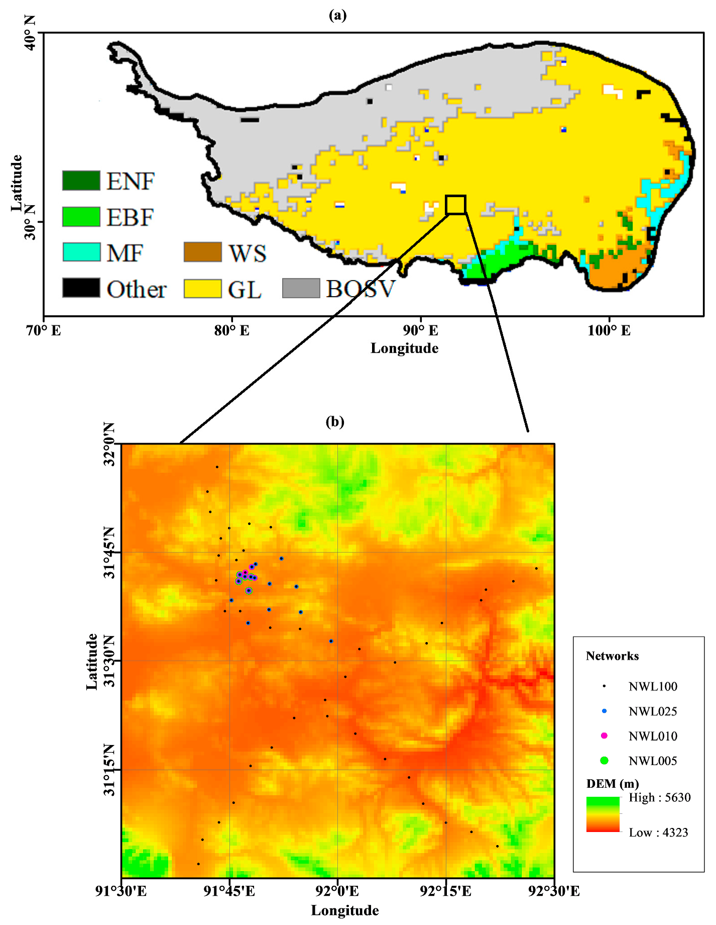
2.1. Study Area

In this study, we chose the TP as the study area. The TP is located between 70°–105° E and 25°–40° N (Figure 1a) and is known as the Earth’s Third Pole and Asia’s water towers. The TP plays an important role in global change and is well characterized by SM. The annual precipitation is 300–700 mm, and 75% of this amount is received from May to October. SM varies seasonally and is low in the winter and high in the summer. The study area land cover from MODIS for 2014 was aggregated from a spatial resolution of 0.05° to 0.25° based on the maximum area ratio and is shown in Figure 1a. The dominant land cover types are “Grassland” and “Barren or Sparsely Vegetated”. For more information about the TP, we refer to Chen et al. [20] and Yang et al. [21].

2.2. Materials

2.2.1. Ground Data

A soil moisture/temperature monitoring network named Naqu network, containing 57 stations, was gradually assembled in the central TP since August 2010 to validate satellite SM products (Figure 1b) [22]. The network is about 100 × 100 km2 and located at 4500 m above sea level. The main sensors are the EC-TM capacitance probes manufactured by Decagon Devices with an accuracy of ±0.03 cm3 cm−3. The influence area of each station is about several square meters. At each station, four such sensors are installed at depths of 5, 10, 20, and 40 cm, respectively, and the sampling frequency was set to once every 30 mins. In this study, we used the ground data collected between 1 January 2014 and 31 December 2014. The daily observations were obtained by averaging the 30-min soil moisture observations at a depth of 5 cm to match the remotely sensed SM. We extracted four validation networks with sizes of 0.05° × 0.05° (NWL005), 0.1° × 0.1° (NWL010), 0.25° × 0.25° (NWL025), 1° × 1° (NWL100) to perform a comprehensive validation (Table 1). The SM values of these four networks were obtained by averaging the stations’ valid soil moisture observations in each network. For more details about the data processing, readers are kindly referred to Chen et al. [20].

2.2.2. FY-3B SM Products

The FY-3B satellite was launched by the China National Space Administration on November 2010 and is equipped with a passive microwave radiometer called Microwave Radiation Imager (MWRI). MWRI provides observations with frequencies ranging from 10.7 GHz to 89.0 GHz in both ascending (1:40 P.M.) and descending (1:40 A.M.) mode. For this study, we used the ascending FY-3B level-3 SM product with a grid resolution of 0.25°and temporal resolution of 2–3 days provided by the Chinese National Satellite Meteorological Center (http://satellite.nsmc.org.cn/portalsite/default.aspx). The FY-3B SM was retrieved from an iterative inversion algorithm using the brightness temperature observations of 10.7 and 18.7 GHz [4]. In the algorithm, the effects of surface temperature and vegetation are corrected from the Ka-band (36.5 GHz) vertical polarized brightness temperature and the Normalized Difference Vegetation Index (NDVI). A new surface emission model Qp proposed by Shi et al. [23] was utilized to correct the effects of surface roughness. Due to satellite orbits and retrieval algorithms, gaps in the products are intrinsic [24].

2.2.3. Multi-source Remote Sensing Data
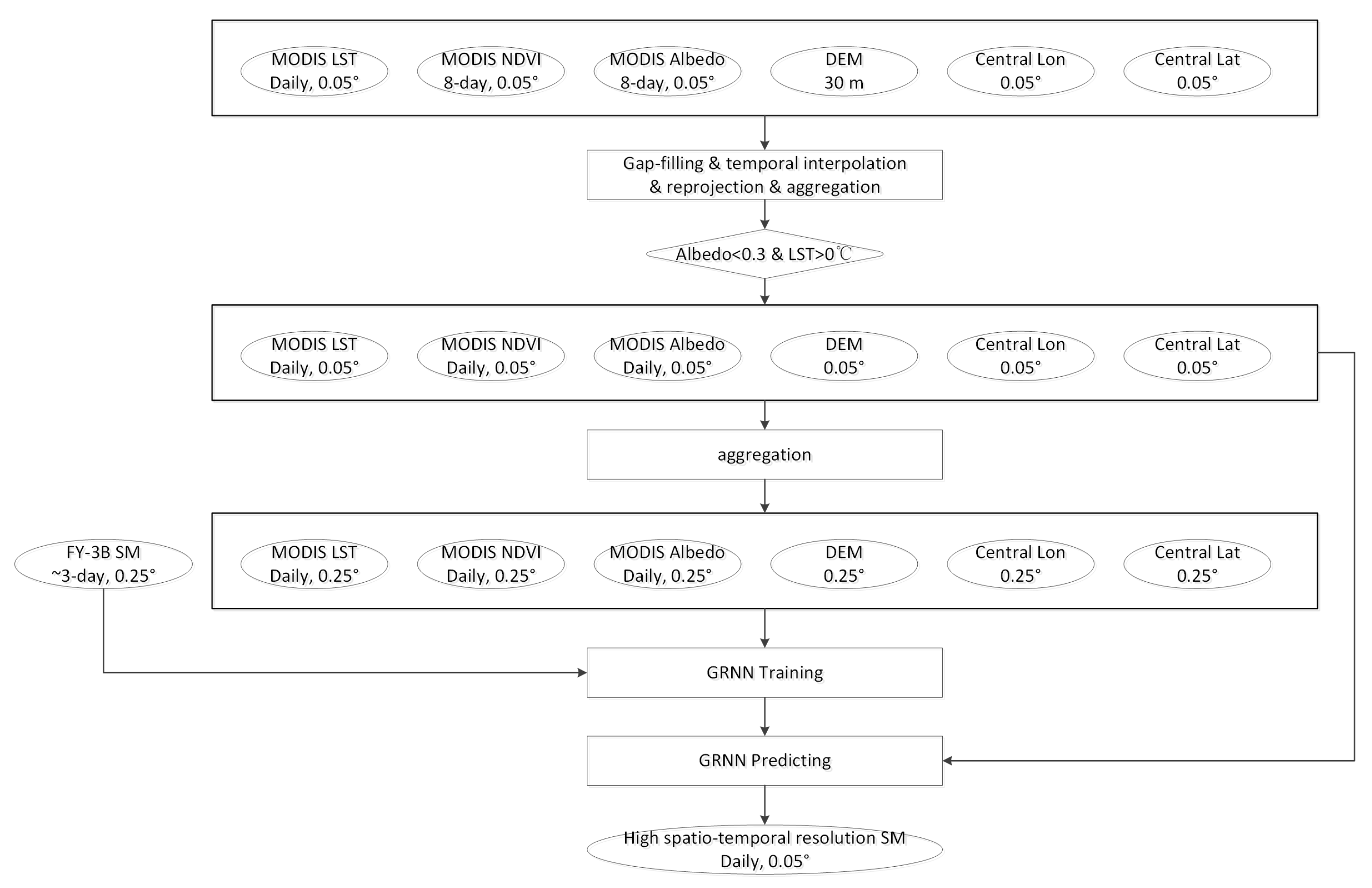
Three MODIS products with a 0.05° spatial resolution, i.e., 8-day NDVI (MOD13C2), daily LST (MOD11C1) and 8-day albedo (MCD43C3) (downloaded from http://reverb.echo.nasa.gov/) for 2014 were used as the reference data in the SM spatio-temporal resolution improving process. One Digital Elevation Model (DEM) from the Shuttle Radar Topography Mission (SRTM) with 30-m resolution was provided by the National Geospatial-Intelligence Agency (NGA), NASA, the Italian Space Agency (ASI) and the German Aerospace Center (DLR) (http://glcf.umd.edu/data/srtm/).

2.3. Methods

The proposed SM spatio-temporal resolution improving algorithm is based on the idea of temporal reconstruction and spatial downscaling. The core objective of the spatio-temporal resolution improving algorithm is to build a linking model between the microwave SM product and the optical products at a low resolution, and then applying it at a high resolution. Hence, building a robust linking model is the most important step in this process. Machine learning models perform better in finding relationships between datasets, especially when these relationships are not easily expressed analytically. In this paper, the General Regression Neural Network (GRNN) was used to obtain high spatio-temporal resolution SM, for the GRNN has a strong fitting ability when limited training data are available. The flowchart (Figure 2) includes four main steps: (1) obtaining high spatio-temporal resolution input variables based on gap-filling methods; (2) obtaining low resolution input variables by simple average method on the high spatio-temporal resolution input variables; (3) training the GRNN at low spatio-temporal resolution; and then (4) putting the high spatio-temporal resolution input variables into the trained GRNN to obtain high spatio-temporal resolution SM. The proposed method is described in detail as follows.

2.3.1. Obtaining High Spatio-Temporal Resolution Input Variables

First, gap-filled LST, NDVI, and albedo with a high spatio-temporal resolution (daily, 0.05°) should be obtained. Due to the influence of the atmosphere and clouds on the optical sensors, there are a lot of erroneous observations in the input variables, here mainly in the MODIS optical products, which need to be identified and removed [25]. The following methods were used to fill the gaps in the input variables [12]. (1) For NDVI, the cloud-free time series was obtained using a two-step Fourier-Transform method called the Harmonic Analysis of Time Series (HANTS) algorithm [25]. The HANTS algorithm [26] is based on the concept of discrete Fourier Transform and was developed to deal with time series of irregularly spaced observations [27]. The HANTS algorithm can also reduce the NDVI temporal resolution from 8-day to 1-day. (2) For LST, a multi-temporal approach proposed by Zeng et al. [28] was implemented to reconstruct the missing “clear sky” LST data based on the hypothesis that the surface temperature of a ground feature only changes linearly over a short time, and similar changes occur on similar features. (3) For albedo, a statistical temporal filtering method was used to generate a gap-filled albedo product [29]. This method is based on the temporal correlation of albedo measurements in neighboring days, which assumes that the true albedo on the k-th day is linearly correlated with the true albedo on the (k+△k)-th day. For albedo, the bilinear interpolation method was used to improve the temporal resolution from 8-days to 1-day. The performance of these methods has been validated by the proposed authors in different study areas. In a previous study, we also qualitatively discussed the usability of these methods over TP, finding that the results of these methods were acceptable. More detailed information can be found in Cui et al. [12].
Second, the DEM is resampled and projected from 30 m to 0.05° and used to eliminate the topographic effects of the LST. The latitude (Lat) and longitude (Lon) of each 0.05° × 0.05° grid center are extracted as the geographic reference data. Unlike the daily LST, NDVI, and albedo, the DEM, Lat and Lon do not change with time. Hence, one map of these three inputs is sufficient.
Remote sensing can only observe soil water in the liquid state. Therefore, the strong relationship between SM and remotely sensed LST, NDVI, and albedo is only found when the soil is unfrozen. In this study, we assume the soil to be unfrozen when the land is not covered by snow (albedo less than 0.3) and the LST is higher than 0 ℃.
Finally, the high spatio-temporal resolution (daily, 0.05°) inputs, including LST, NDVI, albedo, DEM, Lat, and Lon are obtained to be used in the SM spatio-temporal resolution improving algorithm when the soil is unfrozen.

2.3.2. Obtaining Low-Resolution Input Variables

In the relationship finding stage, the spatial resolution of the input variables (LST, NDVI, albedo, DEM, Lat and Lon) should be the same as the SM, which has a low resolution of 0.25°. Hence, we average the daily high spatial resolution input variables to low spatial resolution, i.e., from 0.05° to 0.25°.

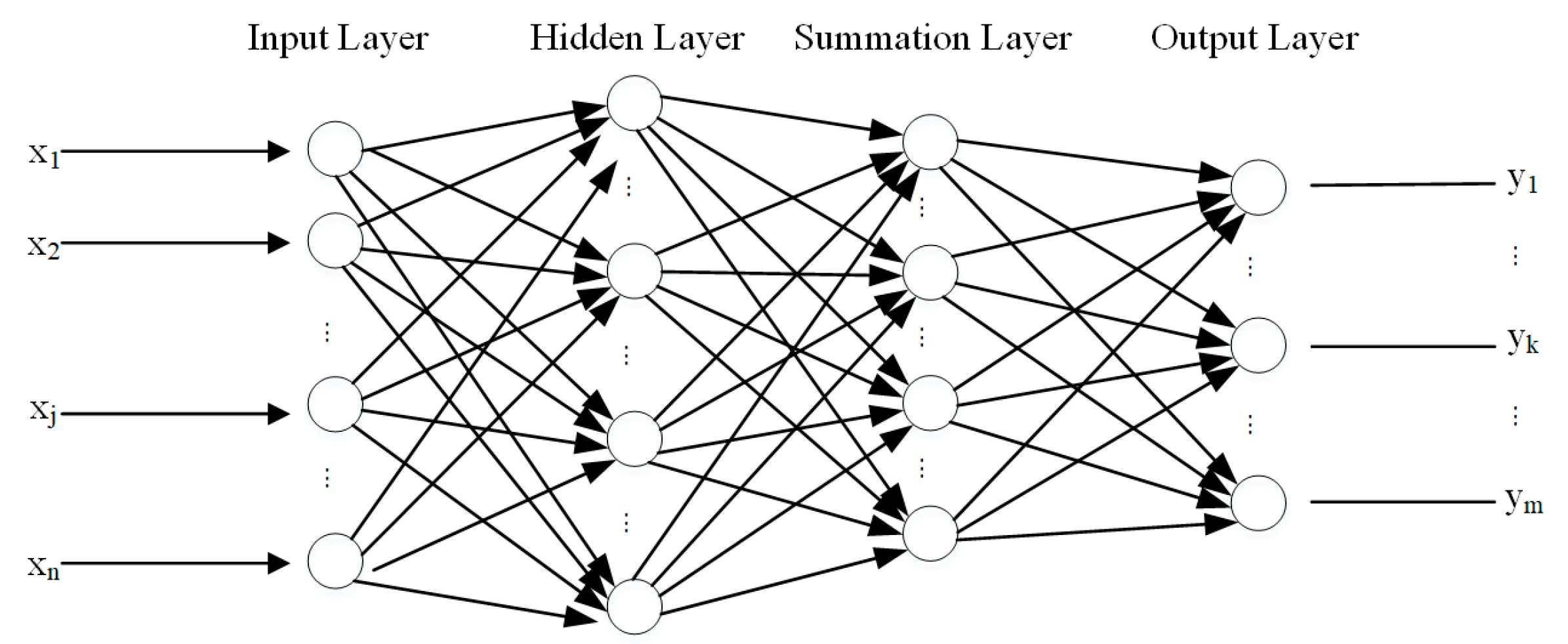
2.3.3. Training GRNN at Low Resolution

GRNN was proposed by Specht in 1991 [30]. The GRNN has four layers, including input layer, hidden layer, summation layer and output layer (as shown in Figure 3). As a kind of radial basis function neural network and a typical machine learning model, GRNN is often used for function approximation to solve regression problems. GRNN has the ability to transform data from a low to a high dimensional space. Hence, it has a strong, non-linear mapping ability with a high degree of fault tolerance and robustness. Studies have shown that the GRNN has greater advantages over BNPP in the ability to approach and learning speed, and can work well with small sample sizes [31].
In this study, we used the GRNN package integrated in the MATLAB software, setting the spread of the radial basis functions to 0.5. The input layer had six nodes (LST, NDVI, albedo, DEM, Lon, Lat) and the output layer had one node (SM). In the training process, the six input variables with low resolution (0.25° and 2–3 day) was used, which has the same spatial resolution of the output. The GRNN was only trained when pixel values were available for both of the input variables and the FY-3B SM product. To improve the performance, a moving window with a size of 2° × 2° was selected. Finally, we obtained a trained GRNN that captured the relationship between the SM and the input variables at the low resolution.

2.3.4. Improving SM Spatio-temporal Resolution

The trained GRNN was driven by the high spatio-temporal resolution input variables to generate high spatio-temporal resolution (0.05° and 1 day) SM. Because the inputs of GRNN were gap-filled and had high resolution, the output SM also had a high spatio-temporal resolution.

2.3.5. Performance Metrics

The performance of the algorithm developed in this study was assessed using standard statistical performance evaluation criteria. The metrics considered included the root mean squared error (RMSE), bias, and unbiased RMSE (ubRMSE), which removes mean bias from the RMSE. Because the data are not a normal distribution (see results), the correlation coefficient is not used in this study. These metrics are defined as follows:
R M S E = 1 N i = 1 N ( S M m S M o ) 2
b i a s = 1 N i = 1 N ( S M m S M o )
u b R M S E = R M S E 2 b i a s 2
where S M m is the estimated SM, S M o is the observed or original SM, S M m ¯ is the average of the estimated SM, S M o ¯ is the average of the observed or original SM and N is the number of observations.

3. Results and Discussions

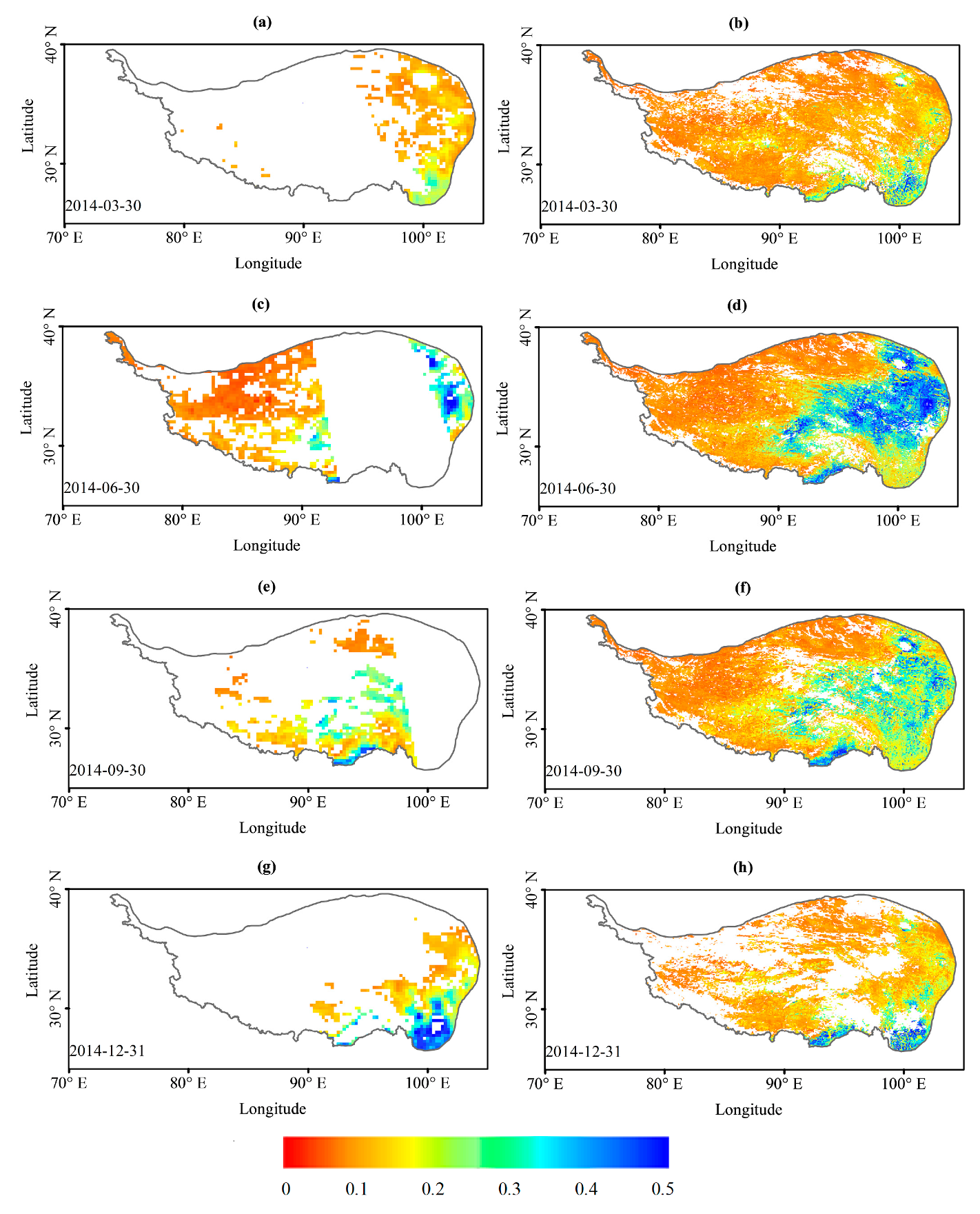
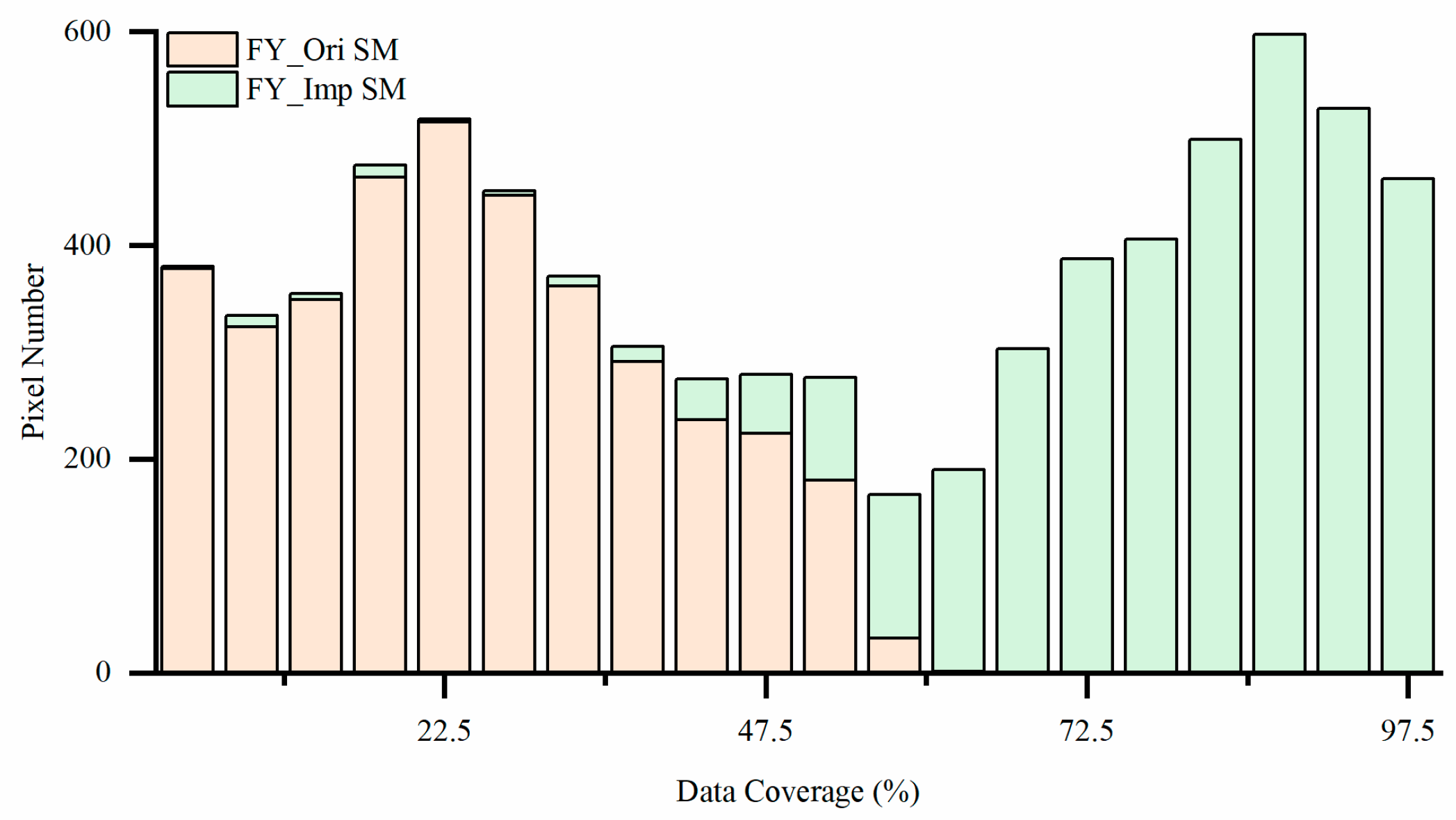
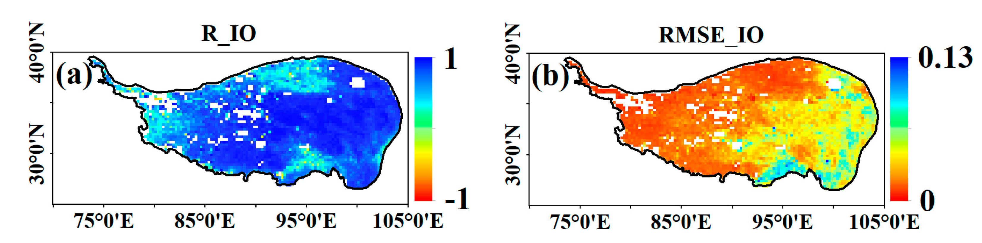
3.1. Spatial Resolution Analysis

The original FY-3B SM (labeled as FY_Ori SM) of 2014 was reconstructed and downscaled to generate high spatio-temporal resolution SM. Maps of FY_Ori SM and the corresponding spatio-temporal resolution-improved SM (labeled as FY_Imp SM) for 30/03, 30/06, 30/09, 31/12 over the TP are shown in Figure 4. The FY_Imp SM improved in terms of spatial details and preserved spatial patterns similar to those of FY_Ori SM over most of the TP. Higher SM was mainly found in the east, especially during the summer. Lower SM was mainly found in the west, especially in the winter. The southeastern TP had high SM all year. From the four figures, we can see that the temporal distribution characteristics of the FY_Imp SM were consistent with FY_Ori SM, increasing from winter to summer. Additionally, the dynamic range of FY_Ori SM was also reproduced in the FY_Imp SM, indicating that the GRNN model has a robust performance. The extremely wet area in the southeastern TP was also captured by the FY_Imp SM. This represents an important improvement with respect to other downscaling algorithms based on soil moisture indices, which fail to capture the characteristic in this region [32].

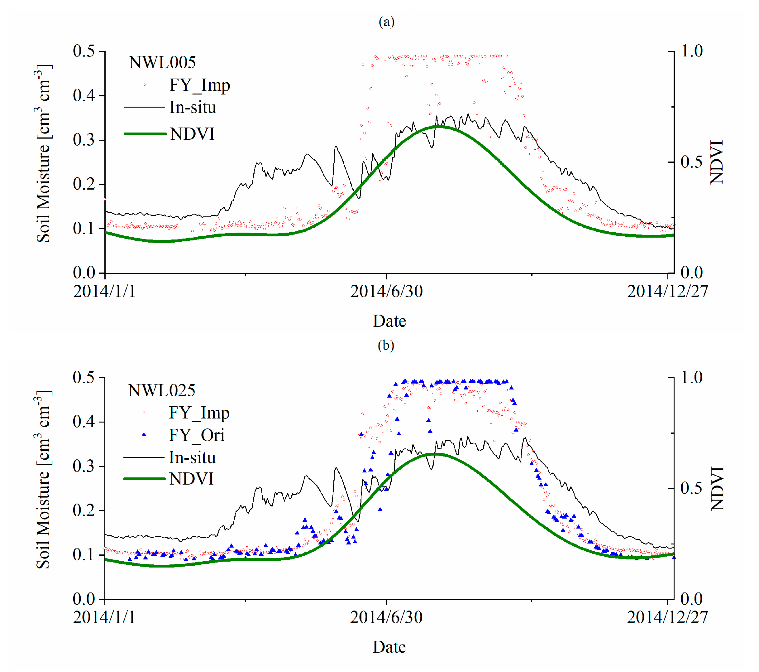
3.2. Temporal Resolution Analysis

From Figure 4 b,d,f,h, we can see that the spatial coverage of FY_Imp SM improves significantly compared with the FY_Ori SM. From Figure 4a,c,e,g, we can see that there are a lot of gaps in the FY_Ori SM, and also find that the gaps are not always due to the orbit or snow/glacier/water cover. The SM retrieval algorithm is another main reason for the gaps. These examples show that the FY_Imp SM completely filled the data gaps in FY_Ori SM when the soil was unfrozen and greatly enriched the spatial details and variations of SM. This represents an important improvement with respect to other spatial downscaling algorithms, which fail to improve the temporal resolution resulting in a large number of gaps in the downscaled SM map [32,33].
The data coverage was calculated after resampling the FY_Imp SM from 0.05° to 0.25°. Figure 5 shows the histograms of the FY_Ori SM and FY_Imp SM data coverages. The coverage of FY_Ori SM is lower than 30% over most of the TP. The entire TP SM coverage was improved from 23.7% to 78.7% with our proposed method. Regardless of the surface covered by water/glaciers or the soil being frozen, FY_Imp SM is temporally continuous at the daily scale.

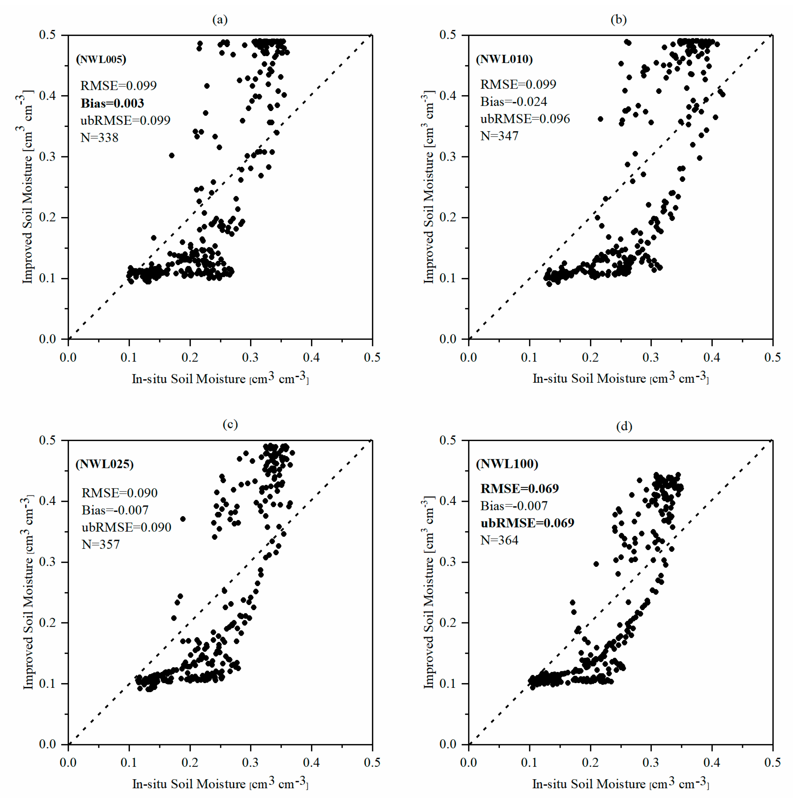
3.3. Comparison with the Original FY-3B Soil Moisture and In Situ Measurements

The FY_Imp SM was resampled from 0.05° to 0.25° and compared with the FY_Ori SM to evaluate its consistency. We calculated the correlation coefficient (R_IO) and RMSE_IO between the resampled FY_Imp and FY_Ori SM and both metrics show different spatial distributions (Figure 6a,b). For the most part of the TP, R_IO is larger than 0.9. Hence, it is reasonable to say that FY_Imp SM is consistent with the FY_Ori SM in its ability of capturing SM variation over the TP. In the north and west, where the soil is dry, the R_IO is lower than other parts but the RMSE_IO is also lower. The main reason for this is that the dynamic range of yearly soil moisture is small, causing the lower model fitting performance. Meanwhile, we can see that higher R_IO does not always result in lower RMSE_IO. For example, in the south of TP, where the soil is wet, the RMSE_IO is higher; an analysis of the input data reveals that here the terrain is complex, with elevations from 100 m to 6000 m in a local 2° × 2° window. This leads to conclude that a global downscaling strategy of the machine learning model is unsuitable to complex terrain regions (results not shown). Hence, we chose a local application strategy with a moving window of 2° × 2° to mitigate the uncertainty in this study. In the high RMSE_ IO region, the results do not support the residual-based correction approach in the spatial resolution downscaling process [33].
In the two large (NWL025 and NWL100) in situ networks, we calculated the error metrics of FY_Ori SM and FY_Imp SM against the in situ observations. From Table 2, we can see that FY_Imp SM is comparable to FY_Ori SM. However, the FY_Imp SM has more observation samples than FY_Ori SM, meaning that the temporal resolution is significantly improved; this is consistent with Section 3.1 and Section 3.2. Compared with the FY_Ori SM, the RMSE and ubRMSE of FY_Imp SM were slightly decreased, thought the absolute bias showed little change. This means that the spatio-temporal resolution-improving process could reduce the statistical error by increasing the number of valid observations. This gives us an indication that satellite-based SM products perform differently when data have different time spans, and a validation based on long-term observations seems more credible. This assumption should be verified in future research.
The FY_Imp SM is validated against the in situ measurements at four different spatial resolution networks (0.05°, 0.1°, 0.25° and 1°), as shown in Figure 7. In all the field networks, the in situ observations and the pixel values were aggregated to the same spatial scale as the field networks to make them comparable. The RMSE, bias and ubRMSE show little change at different scales. As resolution increases, the RMSE and ubRMSE slightly increase. The maximum bias is −0.024 cm3 cm−3, indicating that FY_Imp underestimated SM, just like the FY_Ori SM. For lower bias, ubRMSE is very close to RMSE, and both are larger than that of the new SMAP SM target of 0.04 cm3 cm −3 [5], indicating that the X-band is not the optimal wavelength to retrieve soil moisture compared with the L-band.
Figure 8 shows the time series of FY_Imp and FY_Ori SM compared with in situ SM measurements at networks NWL005 and NWL025. It can be observed that the FY_Imp SM has similar performance with the FY_Ori SM in capturing the temporal dynamics of in situ SM, where the SM is high in summer and low in winter. The FY_Imp SM is mainly determined by the FY_Ori SM and other factors, such as vegetation cover and soil unconsidered freeze/thaw events, have limited effect on the FY_Imp SM. For example, although FY_Imp SM underestimate the in situ value during April-May, it is still highly consistent with the FY_Ori SM. One thing that should be noted is that with the increase of land surface complexity, such as vegetation cover increasing, the consistency between FY_Imp and FY_Ori SM will decrease slightly. Hence, improving the quality of the input data of GRNN is still a key step to further improve the FY_Imp SM quality. Overall, the FY_Imp SM is consistent with the FY_Ori SM and the quality does not decrease in the spatio-temporal resolution improving process.

4. Conclusions

The main objective of this study was to propose a method for obtaining high spatio-temporal resolution SM. The method has two features: (1) it obtains high spatio-temporal resolution SM and (2) it produces results that are consistent with the original SM product. In this study, a GRNN based SM spatio-temporal resolution improvement approach was proposed and validated for unfrozen soil over the TP. The SM spatio-temporal resolution-improving algorithm was evaluated and tested for its reliability and robustness using FY-3B SM over the TP. The FY-3B SM was successfully downscaled from 0.25° to 0.05°, and coverage was improved from 23.7% to 78.7%. The downscaled SM shows more detailed variations in both the spatial and temporal distributions. Additionally, the resolution-improved SM has a strong consistency and quality with the original SM product based on the in situ measurements. The GRNN-based SM spatio-temporal resolution-improving algorithm can also be applied to other satellite SM products with low spatial resolution and a large number of gaps. This will help us understand SM data better, especially under a changing climate.

Author Contributions

Conceptualization, methodology and formal analysis, Y.C.; software, Y.C. and X.C.; validation and visualization, X.C., W.X., F.L. and Z.L.; writing—original draft preparation, Y.C.; writing—review and editing, L.H., W.F. and Y.H. All authors have read and agreed to the published version of the manuscript.

Funding

This study was financially supported by the Key R&D Program of the Ministry of Science and Technology, China (Grant No. 2018YFC1506504, and 2017YFE0122400) and National Science Foundation of China (Grant No. 41901348, and 41701384), and the Strategic Priority Research Program of the Chinese Academy of Sciences (Grant No. XDA19030203).

Acknowledgments

We thank Cristina Milesi for helping to revise the language. We thank Wei Zhao and three anonymous reviewers for their valuable comments to improve this manuscript. We also are grateful to Kun Yang, Chao Zeng and Jie Zhou for kindly providing the in situ data, the gap-filled LST data, the gap-filled NDVI data, respectively.

Conflicts of Interest

The authors declare no conflict of interest.

References

  1. Njoku, E.G.; Jackson, T.J.; Lakshmi, V.; Chan, T.K.; Nghiem, S.V. Soil moisture retrieval from AMSR-E. Geosci. Remote Sens. IEEE Trans. 2003, 41, 215–229. [Google Scholar] [CrossRef]
  2. Wagner, W.; Hahn, S.; Kidd, R.; Melzer, T.; Bartalis, Z.; Hasenauer, S.; Figa-Saldana, J.; de Rosnay, P.; Jann, A.; Schneider, S.; et al. The ASCAT Soil Moisture Product: A Review of its Specifications, Validation Results, and Emerging Applications. Meteorol. Z. 2013, 22, 5–33. [Google Scholar] [CrossRef] [Green Version]
  3. Wigneron, J.P.; Waldteufel, P.; Chanzy, A.; Calvet, J.C.; Kerr, Y. Two-dimensional microwave interferometer retrieval capabilities over land surfaces (SMOS Mission). Remote Sens. Environ. 2000, 73, 270–282. [Google Scholar] [CrossRef]
  4. Parinussa, R.; Wang, G.; Holmes, T.; Liu, Y.; Dolman, A.; de Jeu, R.; Jiang, T.; Zhang, P.; Shi, J. Global surface soil moisture from the Microwave Radiation Imager onboard the Fengyun-3B satellite. Int. J. Remote Sens. 2014, 35, 7007–7029. [Google Scholar] [CrossRef]
  5. Entekhabi, D.; Njoku, E.G.; Neill, P.E.O.; Kellogg, K.H.; Crow, W.T.; Edelstein, W.N.; Entin, J.K.; Goodman, S.D.; Jackson, T.J.; Johnson, J. The Soil Moisture Active Passive (SMAP) Mission. P Ieee 2010, 98, 704–716. [Google Scholar] [CrossRef]
  6. Albergel, C.; Rüdiger, C.; Pellarin, T.; Calvet, J.-C.; Fritz, N.; Froissard, F.; Suquia, D.; Petitpa, A.; Piguet, B.; Martin, E. From near-surface to root-zone soil moisture using an exponential filter: an assessment of the method based on in-situ observations and model simulations. Hydrol. Earth Syst. Sci. Discuss. 2008, 12, 1323–1337. [Google Scholar] [CrossRef] [Green Version]
  7. Jackson, T.J.; Cosh, M.H.; Bindlish, R.; Starks, P.J.; Bosch, D.D.; Seyfried, M.; Goodrich, D.C.; Moran, M.S.; Du, J.Y. Validation of Advanced Microwave Scanning Radiometer Soil Moisture Products. IEEE Trans. Geosci. Remote 2010, 48, 4256–4272. [Google Scholar] [CrossRef]
  8. Zeng, J.; Li, Z.; Chen, Q.; Bi, H.Y.; Qiu, J.X.; Zou, P.F. Evaluation of remotely sensed and reanalysis soil moisture products over the Tibetan Plateau using in-situ observations. Remote Sens. Environ. 2015, 163, 91–110. [Google Scholar] [CrossRef]
  9. Piles, M.; Camps, A.; Vall-Llossera, M.; Corbella, I.; Panciera, R.; Rudiger, C.; Kerr, Y.H.; Walker, J. Downscaling SMOS-derived soil moisture using MODIS Visible/Infrared data. IEEE Trans. Geosci. Remote Sens. 2011, 49, 3156–3166. [Google Scholar] [CrossRef]
  10. Merlin, O.; Chehbouni, A.G.; Kerr, Y.H.; Njoku, E.G.; Entekhabi, D. A combined modeling and multipectral/multiresolution remote sensing approach for disaggregation of surface soil moisture: Application to SMOS configuration. IEEE Trans. Geosci. Remote Sens. 2005, 43, 2036–2050. [Google Scholar] [CrossRef]
  11. Wagner, W.; Dorigo, W.; De Jeu, R.; Fernandez, D.; Benveniste, J.; Haas, E.; Ertl, M. Fusion of Active and Passive Microwave Observations to Create AN Essential Climate Variable Data Record on Soil Moisture. ISPRS Ann. 2012, I-7, 315–321. [Google Scholar]
  12. Cui, Y.; Long, D.; Hong, Y.; Zeng, C.; Zhou, J.; Han, Z.; Liu, R.; Wan, W. Validation and reconstruction of FY-3B/MWRI soil moisture using an artificial neural network based on reconstructed MODIS optical products over the Tibetan Plateau. J. Hydrol. 2016, 543, 242–252. [Google Scholar] [CrossRef]
  13. Peng, J.; Loew, A.; Merlin, O.; Verhoest, N.E. A review of spatial downscaling of satellite remotely sensed soil moisture. Rev. Geophys. 2017, 55, 341–366. [Google Scholar] [CrossRef]
  14. Merlin, O.; Chehbouni, A.; Walker, J.P.; Panciera, R.; Kerr, Y.H. A simple method to disaggregate passive microwave-based soil moisture. IEEE Trans. Geosci. Remote Sens. 2008, 46, 786–796. [Google Scholar] [CrossRef] [Green Version]
  15. Chauhan, N.S.; Miller, S.; Ardanuy, P. Spaceborne soil moisture estimation at high resolution: A microwave-optical/IR synergistic approach. Int. J. Remote Sens. 2003, 24, 4599–4622. [Google Scholar] [CrossRef]
  16. Merlin, O.; Walker, J.P.; Chehbouni, A.; Kerr, Y. Towards deterministic downscaling of SMOS soil moisture using MODIS derived soil evaporative efficiency. Remote Sens. Environ. 2008, 112, 3935–3946. [Google Scholar] [CrossRef] [Green Version]
  17. Wei, Z.; Li, A. A comparison study on empirical microwave soil moisture downscaling methods based on the integration of microwave-optical/IR data on the Tibetan Plateau. Int. J. Remote Sens. 2015, 36, 4986–5002. [Google Scholar]
  18. Srivastava, P.K.; Han, D.; Ramirez, M.R.; Islam, T. Machine Learning Techniques for Downscaling SMOS Satellite Soil Moisture Using MODIS Land Surface Temperature for Hydrological Application. Water Resour. Manag. 2013, 27, 3127–3144. [Google Scholar] [CrossRef]
  19. Remesan, R.; Shamim, M.A.; Han, D.; Mathew, J. Runoff prediction using an integrated hybrid modelling scheme. J. Hydrol. 2009, 372, 48–60. [Google Scholar] [CrossRef]
  20. Chen, Y.; Yang, K.; Qin, J.; Long, Z.; Tang, W.; Han, M. Evaluation of AMSR-E retrievals and GLDAS simulations against observations of a soil moisture network on the central Tibetan Plateau. J. Geophys. Res. Atmos. 2013, 118, 4466–4475. [Google Scholar] [CrossRef]
  21. Yang, K.; Wu, H.; Qin, J.; Lin, C.; Tang, W.; Chen, Y. Recent climate changes over the Tibetan Plateau and their impacts on energy and water cycle: A review. Glob. Planet. Chang. 2014, 112, 79–91. [Google Scholar] [CrossRef]
  22. Yang, K. A Multi-Scale Soil Moisture and Freeze-Thaw Monitoring Network on the Tibetan Plateau and Its Applications. Bull. Am. Meteorol. Soc. 2013, 94, 1907–1916. [Google Scholar] [CrossRef]
  23. Shi, J.C.; Jiang, L.M.; Zhang, L.X.; Chen, K.S.; Wigneron, J.P.; Chanzy, A.; Jackson, T.J. Physically based estimation of bare-surface soil moisture with the passive radiometers. IEEE Trans. Geosci. Remote Sens. 2006, 44, 3145–3153. [Google Scholar] [CrossRef]
  24. Dorigo, W.; Wagner, W.; Albergel, C.; Albrecht, F.; Balsamo, G.; Brocca, L.; Chung, D.; Ertl, M.; Forkel, M.; Gruber, A.; et al. ESA CCI Soil Moisture for improved Earth system understanding: State-of-the art and future directions. Remote Sens. Environ. 2017, 203, S0034425717303061. [Google Scholar] [CrossRef]
  25. Jia, L.; Shang, H.; Hu, G.; Menenti, M. Phenological response of vegetation to upstream river flow in the Heihe Rive basin by time series analysis of MODIS data. Hydrol. Earth Syst. Sci. 2011, 15, 1047–1064. [Google Scholar] [CrossRef] [Green Version]
  26. Menenti, M.; Azzali, S.; Verhoef, W.; Vanswol, R. Mapping Agroecological Zones and Time-Lag in Vegetation Growth by Means Of Fourier-Analysis Of Time-Series Of Ndvi Images. Adv. Space Res. 1993, 13, 233–237. [Google Scholar] [CrossRef]
  27. Jia, L.; Xi, G.; Liu, S.; Huang, C.; Yan, Y.; Liu, G. Regional estimation of daily to annual regional evapotranspiration with MODIS data in the Yellow River Delta wetland. Hydrol. Earth Syst. Sci. 2009, 13, 1775–1787. [Google Scholar] [CrossRef] [Green Version]
  28. Zeng, C.; Shen, H.; Zhong, M.; Zhang, L.; Wu, P. Reconstructing MODIS LST based on multitemporal classification and robust regression. Geosci. Remote Sens. Lett. IEEE 2015, 12, 512–516. [Google Scholar] [CrossRef]
  29. Liu, N.F.; Liu, Q.; Wang, L.Z.; Liang, S.L.; Wen, J.G.; Qu, Y.; Liu, S.H. A statistics-based temporal filter algorithm to map spatiotemporally continuous shortwave albedo from MODIS data. Hydrol. Earth Syst. Sci. 2013, 17, 2121–2129. [Google Scholar] [CrossRef] [Green Version]
  30. Specht, D.F. A general regression neural network. IEEE Trans. Neural Netw. 1991, 2, 568–576. [Google Scholar] [CrossRef] [Green Version]
  31. Ding, S.; Chang, X.H.; Wu, Q.H. A Study on Approximation Performances of General Regression Neural Network. Appl. Mech. Mater. 2014, 441, 713–716. [Google Scholar] [CrossRef]
  32. Wei, Z.; Meng, Y.; Zhang, W.; Peng, J.; Meng, L. Downscaling SMAP soil moisture estimation with gradient boosting decision tree regression over the Tibetan Plateau. Remote Sens. Environ. 2019, 225, 30–44. [Google Scholar] [CrossRef]
  33. Jing, W.; Zhang, P.; Zhao, X. Reconstructing Monthly ECV Global Soil Moisture with an Improved Spatial Resolution. Water Resour. Manag. 2018, 32, 2523–2537. [Google Scholar] [CrossRef]
Figure 1. Study area: (a) MODIS land cover types aggregated to 0.25° over the Tibetan Plateau, where EF: Evergreen Needleleaf Forest; EBF: Evergreen Broadleaf Forest; MF: Mixed Forest; WS: Woody Savannas; GL: Grasslands; BOSV: Barren or Sparsely Vegetated. and (b) Naqu soil moisture monitoring network and the distribution of measuring stations based on the Digital Elevation Model map, where NWL100, NWL025, NWL010 and NWL005 are four filed networks with size of 1° × 1°, 0.25° × 0.25°, 0.10° × 0.01°, 0.05° × 0.05°.
Remotesensing 12 00455 g001
Figure 2. Flowchart of the soil moisture spatio-temporal resolution improving algorithm based on the General Regression Neural Network (GRNN) model using the FY-3B product.
Remotesensing 12 00455 g002
Figure 3. GRNN block diagram. X = [x1, x2, …, xn] is the input vector, Y = [y1, yk, …, ym] is the output vector.
Remotesensing 12 00455 g003
Figure 4. Maps of Fengyun original soil moisture (FY_Ori SM, left column: (a,c,e,g)), and corresponding resolution-improved soil moisture (FY_Imp SM, right column: (b,d,f,h)) on 30/03, 30/06, 30/09, 31/12, over the Tibetan Plateau. Units: cm3 cm−3.
Remotesensing 12 00455 g004
Figure 5. Histograms of data coverage (in %) for FY_Ori SM and FY_Imp SM over the Tibetan Plateau.
Remotesensing 12 00455 g005
Figure 6. Difference between FY_Imp and FY_Ori SM: (a,b) are correlation coefficient (R_IO) and RMSE_IO between FY_Imp and FY_Ori soil moisture, respectively. The unit of RMSE_IO is cm3 cm−3.
Remotesensing 12 00455 g006
Figure 7. Scatter plots of FY_Imp SM against in situ SM measurements at four field SM networks. Error metrics are all in cm3 cm−3 and include: RMSE (root mean square error), Bias (mean bias) and ubRMSE (unbiased RMSE), N (the number of samples). The numbers in bold represent the best results for each error metric.
Remotesensing 12 00455 g007
Figure 8. Time series of FY_Imp soil moisture (SM) and FY_Ori SM compared with in situ measurements for 2014. (a) FY_Imp SM at NWL005; (b) FY_Ori and FY_Imp SM at NWL025.
Remotesensing 12 00455 g008
Table 1. Number of stations in the four validation networks.
Network NameNumber of StationsDepth (cm)
NWL00555
NWL01085
NWL025145
NWL100575
Table 2. Error metrics of FY_Ori SM and FY_Imp SM against the in situ observations. RMSE (root mean square error), Bias (mean bias) and ubRMSE (unbiased RMSE) are all in cm3 cm−3, N is the number of samples.
SourceNetworkRMSEBiasubRMSEN
FY_Ori

FY_Imp
NWL0250.102−0.0070.102170
NWL1000.082−0.0070.082191
NWL0250.090−0.0070.090357
NWL1000.069−0.0070.069364

