Bidirectional Segmented Detection of Land Use Change Based on Object-Level Multivariate Time Series
by
 ,
,
Yuzhu Hao
1,2, 
Zhenjie Chen
1,2,3,*,
Qiuhao Huang
1,2,
Feixue Li
1,2,
Beibei Wang
1,2 and
Lei Ma
1,2 1
School of Geography and Ocean Science, Nanjing University, Nanjing 210023, China
2
Key Laboratory for Satellite Mapping Technology and Applications of State Administration of Surveying, Mapping and Geoinformation, Nanjing University, Nanjing 210023, China
3
Collaborative Innovation Center of Novel Software Technology and Industrialization, Nanjing 210023, China
*
Author to whom correspondence should be addressed.
Remote Sens. 2020, 12(3), 478; https://0-doi-org.brum.beds.ac.uk/10.3390/rs12030478
Submission received: 3 January 2020
/
Revised: 28 January 2020
/
Accepted: 31 January 2020
/
Published: 3 February 2020
(This article belongs to the Special Issue Multitemporal Land Cover and Land Use Mapping)
Abstract
:High-precision information regarding the location, time, and type of land use change is integral to understanding global changes. Time series (TS) analysis of remote sensing images is a powerful method for land use change detection. To address the complexity of sample selection and the salt-and-pepper noise of pixels, we propose a bidirectional segmented detection (BSD) method based on object-level, multivariate TS, that detects the type and time of land use change from Landsat images. In the proposed method, based on the multiresolution segmentation of objects, three dimensions of object-level TS are constructed using the median of the following indices: the normalized difference vegetation index (NDVI), the normalized difference built index (NDBI), and the modified normalized difference water index (MNDWI). Then, BSD with forward and backward detection is performed on the segmented objects to identify the types and times of land use change. Experimental results indicate that the proposed BSD method effectively detects the type and time of land use change with an overall accuracy of 90.49% and a Kappa coefficient of 0.86. It was also observed that the median value of a segmented object is more representative than the commonly used mean value. In addition, compared with traditional methods such as LandTrendr, the proposed method is competitive in terms of time efficiency and accuracy. Thus, the BSD method can promote efficient and accurate land use change detection.
1. Introduction
Land use patterns have changed significantly in recent decades owing to global changes [1,2]. Although various applications have been used to monitor land use change, many challenges exist in extracting dynamic information on land use change over large areas and with a high frequency [3]. With the development of new remote sensing platforms and sensors, significant progress has recently been made in overcoming technical barriers [4]. Rich historical archives of remote sensing images have also made the long-term detection and modeling of land use change possible [5]. Many studies have been conducted to obtain accurate information on the location, time, and type of land use change using remote sensing image time series (TS) [6,7]. TS analysis has unique advantages, especially with regard to its ability to detect changes in vegetation phenology and land use [8,9].
Among the various TS analysis methods, the pixel-level TS analysis of remote sensing images is the most popular. In this method, a TS is constructed for various phases of every pixel based on a particular index, such as the normalized difference vegetation index (NDVI). Then, by comparing the level of similarity between the TS of the various pixels and that of known change types, it is possible to determine the type and time of change from the pixels [10]. This method has been successfully applied to the TS of various images, including Synthetic Aperture Radar (SAR) [11], Landsat [12], and Moderate Resolution Imaging Spectroradiometer (MODIS) [13]. Dynamic time warping (DTW) is a similarity measure that exploits the temporal distortions between two TSs. The concept of DTW was introduced by Sakoe and Chiba [14] to implement automatic speech recognition. DTW, which measures the optimal global alignment between two TSs, is one of the most frequently used methods to quantify the similarity between two series that are not necessarily equal in size [15]. Research has shown that this algorithm, which is based on nonlinear bending, can achieve high matching accuracy [16]. To replace the Euclidean distance and improve classification accuracy, the DTW distance can be integrated into many classification techniques, including nearest neighbors classifiers, support vector machines, and neural networks [17,18]. In addition, DTW can effectively overcome the time alignment problems caused by missing or low-quality data in the long TS classification process [19]. It has been successfully used in satellite image TS analysis [20], classification [21,22,23], and land-use/land-cover (LULC) mapping [24,25]. Many of the aforementioned methods use a single index to measure the similarity of TS, which highly depends on the accuracy of the selected sample points, and cannot detect the change time. However, given the variety of land use types and the uncertainty of temporal nodes, it is difficult to accurately select samples for all types and times of change for the long-term study of land use change. This, in turn, affects the accuracy of change detection. Moreover, detecting land use changes based on pixel-level TS has stringent requirements for the registration accuracy and radiation correction of the remote sensing images. The results also contain significant salt-and-pepper noise, which limits the application potential of the approach [26,27].
Object-level TS of remote sensing images—another type of analysis method—treats each homogeneous object generated via image segmentation as a whole; this better addresses the aforementioned limitations of pixel-level TS methods [28,29]. Two typical methods are often used for object-level change detection: change detection based on synchronous segmentation and change detection after classification. In the first method, multitemporal data are successively superimposed to generate homogeneous objects of similar shapes, sizes, and positions from multitemporal images. This occurs simultaneously with the segmentation and extraction of image objects. The accuracy of this method is highly dependent on the registration accuracy of the multitemporal data [30]. Additionally, the segmentation results often contain objects that are oversegmented or have incomplete boundaries. This is due to the characteristic parameters of multitemporal images that are simultaneously used during segmentation, increasing heterogeneity. Therefore, postprocessing is required to improve the results. In the second method, object-level classifications of images from different phases are performed separately before a comparative analysis. Then, information on categories, geometries, and spatial contexts of the objects is used to determine the changed objects [30,31].
Many studies focus on analyzing the characteristics of the TS of each segmented object to detect changes in land use [32]. The object-level TS method has advantages over the pixel-level TS method in terms of precision [33,34,35]. Nevertheless, many challenges remain. First, the mean value of all pixels within each object is generally selected to represent the object’s representative feature in the TS. The use of the mean weakens the characteristics of the majority of pixels because pixels close to the object’s edge are less representative. This, in turn, reduces the discriminability between the object and other objects [36,37]. Second, the types and times of land use change vary in general. To ensure accuracy, samples for all types and times of change must be selected and used in the detection of change. This is a difficult task to implement. Therefore, detection methods based on incomplete samples cannot accurately identify the type and time of complex land use change [38,39].
To address the challenges outlined above and detect the types and times of land use change from Landsat images, we propose bidirectional segmented detection (BSD) based on object-level multivariate TS. The proposed method uses the median of an object because the median value of a segmented object is more representative than the commonly used mean value. Based on the three-dimensional (3D) DTW TS similarity measurement method with forward and backward detection, our approach adapts to different types and times of land use change and reduces the difficulty of sample selection. We mainly solve the problem of detecting the change time and change type of land use at the same time without using the changed samples. The main contributions of this study are (1) use of the median instead of the mean as the representative feature of objects and (2) combining forward and backward detection processes to detect different types and times of land use change.
2. Study Area and Data
2.1. Study Area
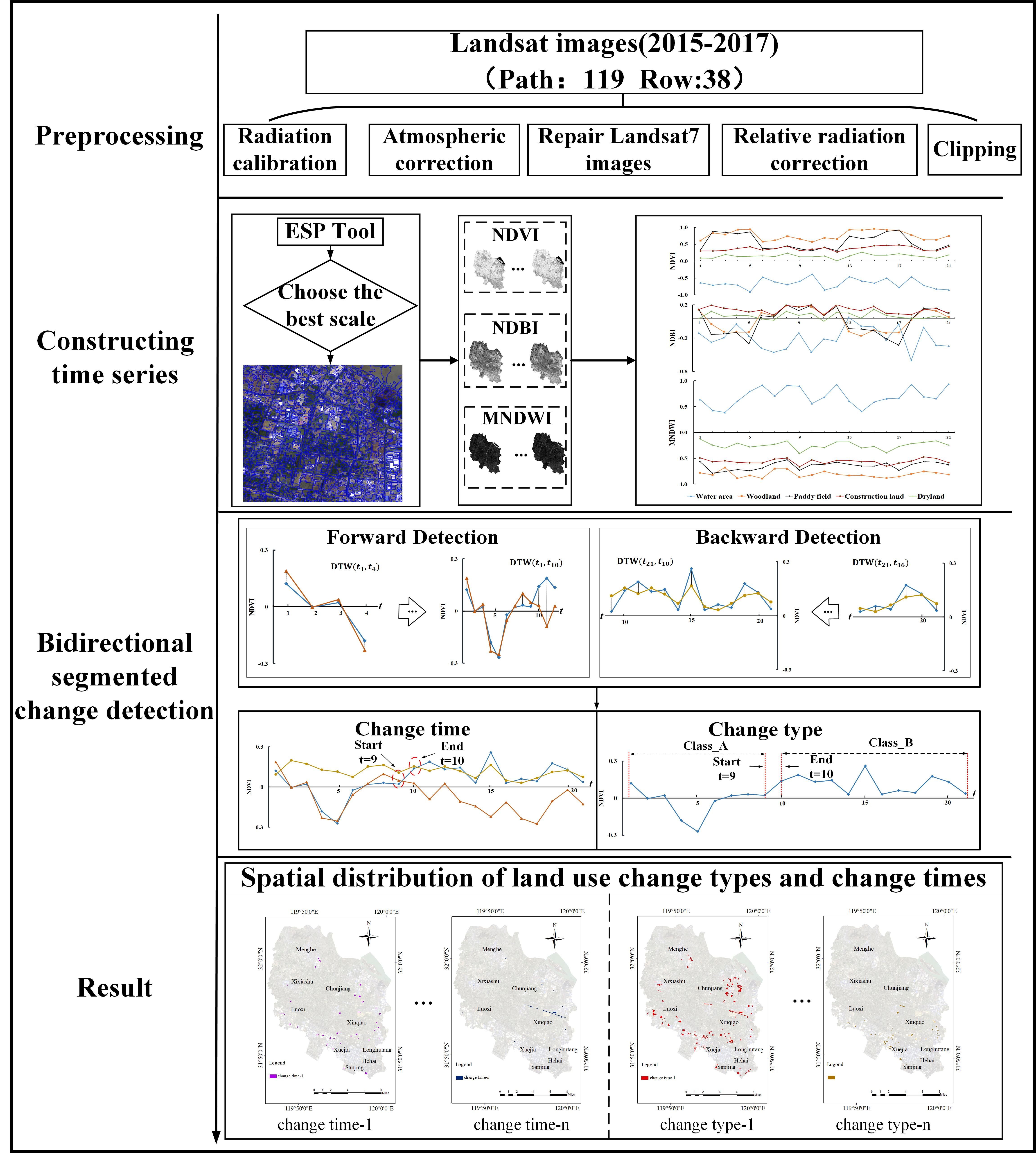
The study area was the Xinbei District of Changzhou City (31°48′–32°03′N and 119°46′–120°01′E) located in the middle of the Yangtze River Delta, China (Figure 1). It is among China’s first batch of national new- and high-tech industrial development zones. The gross domestic product (GDP) in 2016 was 115.503 billion Chinese Yuan, of which 52% was from secondary industries. Rapid urbanization and industrialization in recent years have led to significant changes in regional land use. Land use changes in the Xinbei District are both typical and diverse. Conversions occur not only between the various subtypes of agricultural lands (e.g., conversion from paddy fields to garden lands) but also between construction lands and agricultural lands or between construction lands and water areas.
2.2. Data
All remote sensing images used in this study were downloaded from the official website of the United States Geological Survey (https://earthexplorer.usgs.gov/). These images were acquired by the Landsat 7 Enhanced Thematic Mapper Plus (ETM+) and Landsat 8 Operational Land Imager (OLI) sensors in 2015–2017 from orbit path 119 and row 38. The images of these years were selected as experimental data because the research area developed rapidly during this period; in this dataset, land conversion was frequent, and the number of images in the study area is sufficient, with few images affected by clouds. Among the images, 21 Landsat images of the study area were selected as experimental data (Table 1).
3. Methodology
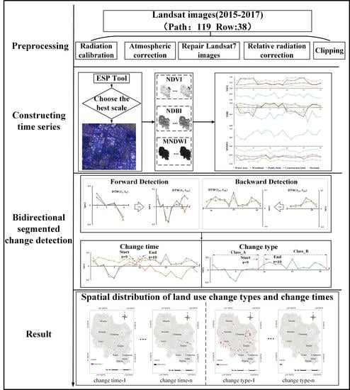
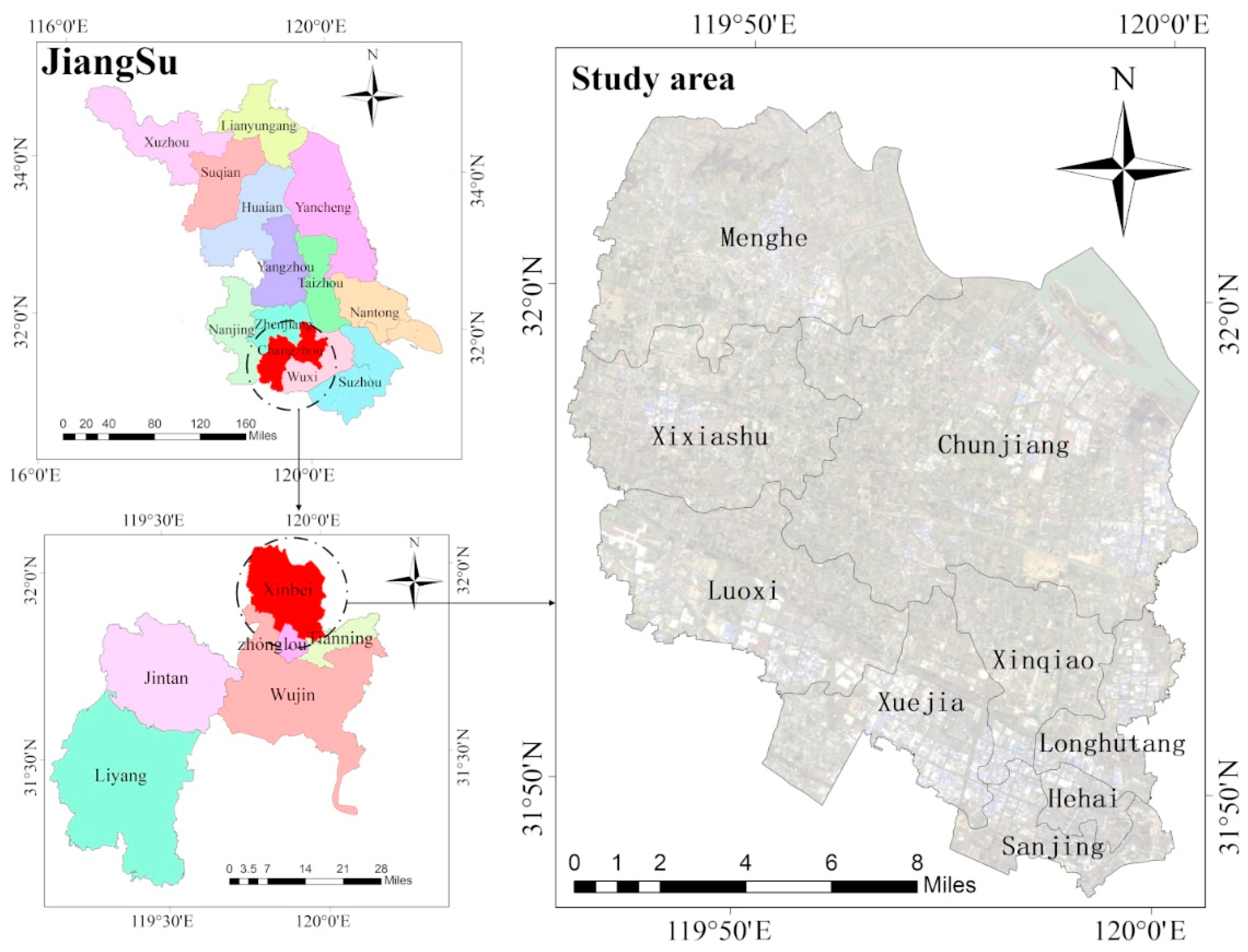
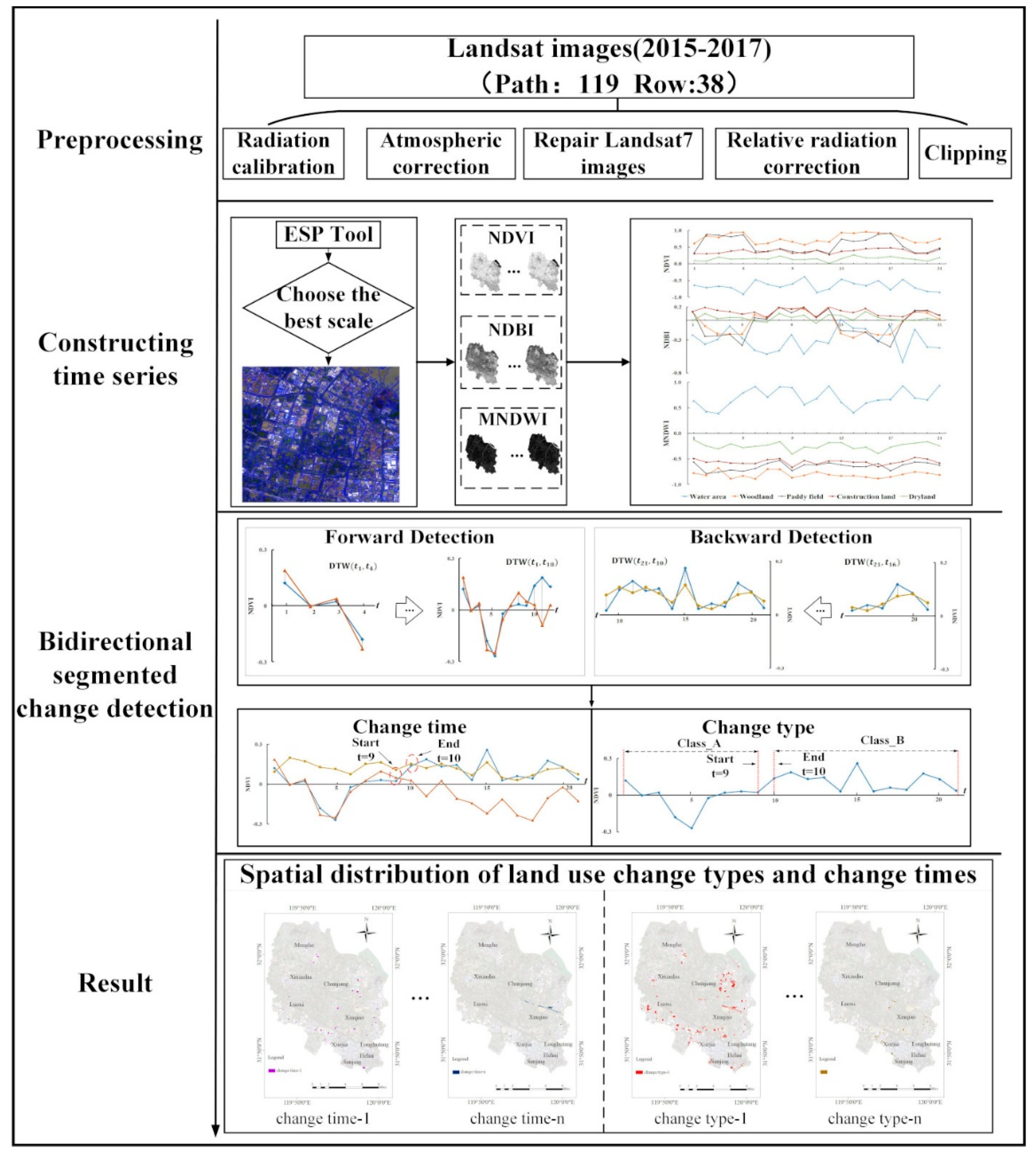
3.1. Overall Method Concept
We proposed a method based on the analysis of object-level multivariate TS for remote sensing detection in the context of land use change. This method first constructs the object-level NDVI, the normalized difference built index (NDBI), and the modified normalized difference water index (MNDWI) TS. Then, the 3D DTW distance is used to measure the similarity and detect the time and type of land use change via segmentation (Figure 2).
The main process involves the following steps:
- (1)
- Preprocess remote sensing images: This includes radiation and atmospheric corrections, gap-filling, and image clipping.
- (2)
- Construct object-level multivariate TS: Remote sensing images of typical phases are selected for the multiresolution segmentation of the images into several homogeneous objects. The NDVI, NDBI, and MNDWI are then used to construct the TS. The median is used instead of the mean as the representative feature of the objects.
- (3)
- Perform BSD on the segmented objects: The TS of unchanged objects of various land uses are chosen as the sample TS. Then, a sample TS curve most similar to the TS pending detection is screened. Next, forward and backward detections are used to determine the time and type of land use change.
3.2. Preprocessing of Remote Sensing Images
Preprocessing of the images involves radiometric calibration, atmospheric correction, gap-filling, and image clipping. To ensure consistency among different sensors and dates, we performed atmospheric correction and radiometric calibration using the Landsat Ecosystem Disturbance Adaptive Processing System (LEDAPS) for each Landsat image [40,41]. Failure of the scan line corrector (SLC) on the Landsat 7 ETM+ resulted in stripes in images acquired after June 2003, which affects the results of the TS analysis. The stripes were filled using the ENVI gap-fill plug-in [42,43,44,45].
3.3. TS Construction Based on Object Characteristics
3.3.1. Multiresolution Segmentation Using TS Images
Prior to TS construction, objects with greater homogeneity should be extracted using the segmentation algorithm from the series of remote sensing images. The segmentation algorithm is a bottom-up growth algorithm [46]. It begins searching for the growth point of an object from the pixel of an image and follows the principle of minimum heterogeneity to find neighboring objects. Before searching for the next object, areas or pixels with the least amount of heterogeneity are merged into one area. Growth is halted upon reaching the maximum heterogeneity value set by the user. When segmenting the series of remote sensing images, multitemporal images are first stacked in time order to form a multiband image; then, the multiband image is segmented.
For multiresolution segmentation, numerous studies have demonstrated the importance of the scale parameter. The scale parameter controls the dimension and size of segmented objects, which may directly affect subsequent results [47,48,49]. In numerous applied studies, land-cover extraction mainly relied on a trial-and-error approach, with segmentation scale parameters determined based on previous experience [50]. However, this approach has been deemed inadvisable [51]; other researchers have since proposed methods to determine optimal segmentation scale parameters [51,52,53]. As one such successful approach to scale optimization, Local Variance (LV) and Rates of Change of LV (ROC-LV) can be combined to determine appropriate segmentation scales [54]; the corresponding Estimate Scale Parameter (ESP) tool was made public for optimizing scale parameters and has been successfully implemented in the eCognition software.
Here, image segmentation was performed using the eCognition software, with which the ESP was used as an evaluation tool to obtain the optimal segmentation scale. The ESP was used to calculate the LV of homogeneous objects in images under different segmentation scale parameters and then to determine the optimal scale parameter for object segmentation using the change rates of the LV. When the change rate was at its largest, the corresponding scale was considered the optimal segmentation scale
The images of all time phases are stacked in chronological order to form a new image with 126 bands, in which the bands selected by the LET7 image are Bands 1–5 and Band 7, and the bands selected by LC8 are Bands 2–7. In the eCognition software, the multiresolution segmentation method was adopted. First, the covariance and variance matrixes were calculated for all pixels of the image according to the band, and then, the correlation coefficient between the bands was obtained [55]. The image layers were set to one for all bands to avoid any bias [56,57,58,59]. Then, the segmentation parameter was selected and the shape parameters and compactness parameters were determined via trial-and-error [58,60,61]. The specific process included first setting the range of shape and compactness to 0.1–0.9 and the change step to 0.1. Then, some buildings and paddy fields in the image were randomly selected and vectorized as the reference segments. Subsequently, various combinations were made, and their results were compared to those of the reference segments. Finally, the ESP tool was used to test the images of the study area and estimate the optimal segment parameters.
3.3.2. Construction of Multivariate TS
When constructing the TS, the selected indices must be capable of clearly distinguishing between various land uses. The five land use types considered in this study were water area, woodland, paddy field, construction land, and dry land (Table 2). NDVI, NDBI, and MNDWI are commonly used indices for analyzing Landsat images [7,60]. NDVI can be used to separate land with dense vegetation cover from that with other uses. NDBI can be used to distinguish construction land. MNDWI is effective at determining water areas and distinguishing them from shadows. Therefore, these three indices were selected for constructing the multivariate TS in this study. The NDVI, NDBI, and MNDWI were calculated using Equations (1)–(3), respectively.
where NIR, R, and MIR represent the near-infrared red, red, and mid-infrared bands, respectively; and Green is the green band.
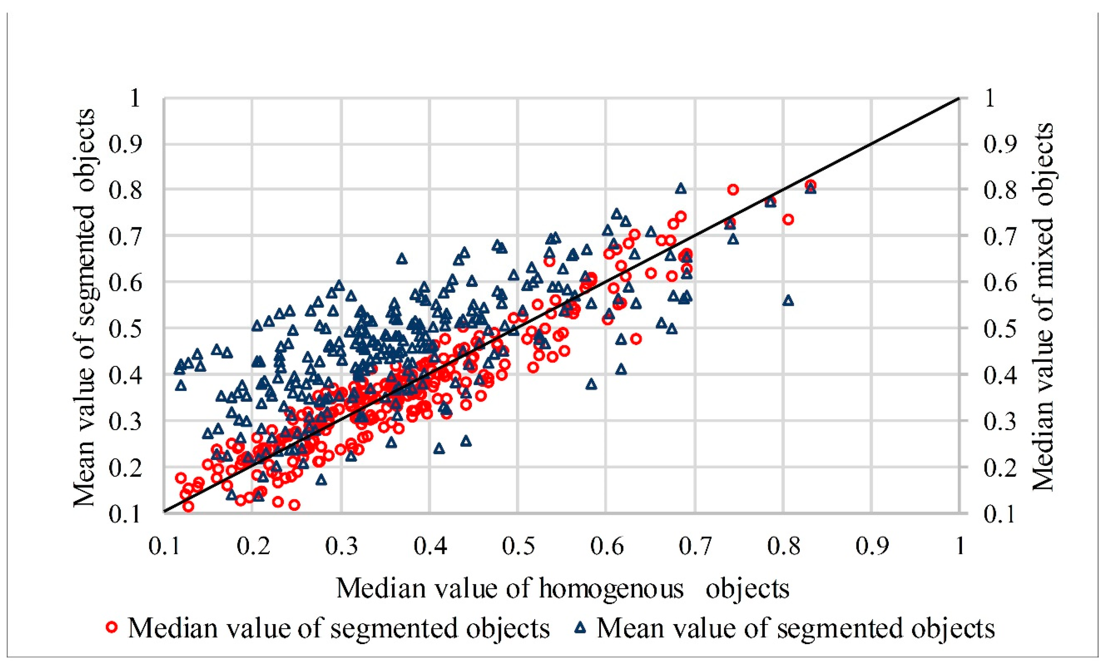
Objects generated via image segmentation often contain many pixels with different index values. Such differences are especially prominent in the index values of pixels at an object’s edge versus that of internal pixels. The segmentation results show that there are many mixed pixels in the segmented objects in the construction land. We choose four mixed samples of construction land to compare the mean and median NDVI value of pixels in the objects. Meanwhile, we choose the samples of nonconstruction area (woodland land, water area, dry land, and paddy field) for comparison (Table 3). For each sample, we manually selected a homogenous object of majority pixels within the segmented boundary (indicated by a yellow line). The experimental results show that the mean and median NDVI values of nonconstruction land are almost the same because the mixed pixels in the segmented objects of nonconstruction land are fewer. For each sample of construction land, the mean NDVI values of a multiresolution segmented object and a homogenous object are quite different, whereas their median NDVI values are almost the same. To further validate the results, we selected 300 segmented objects and corresponding homogenous objects of construction land for statistics. Figure 3 shows that the median NDVI values of segmented objects are closer to the mean NDVI values of corresponding homogenous objects. Therefore, the median value of the segmented object is more representative than the commonly used mean value.
Most existing studies on object-level TS use the mean index of all pixels in an object as the representative feature [61,62]. However, this does not reflect the major characteristics of the object’s index. The median index of pixels is more representative because it better reflects the index characteristics of the majority of pixels in the object and reduces the influence of outliers or noise, especially for construction land (Table 3). Therefore, the median index was used to construct the TS.
3.4. BSD of Segmented Object
3.4.1. BSD Concept
When an object undergoes a land use change, it is necessary to detect the time and type of that change. For shorter time spans (i.e., within 10 years), there is usually one change in land use, such as the conversion of paddy fields to construction land [63,64,65]. For such cases, the land use at the beginning and the end of the TS clearly indicate the type of change. The BSD method proposed in this study can simultaneously detect information in two dimensions: change time and change type.
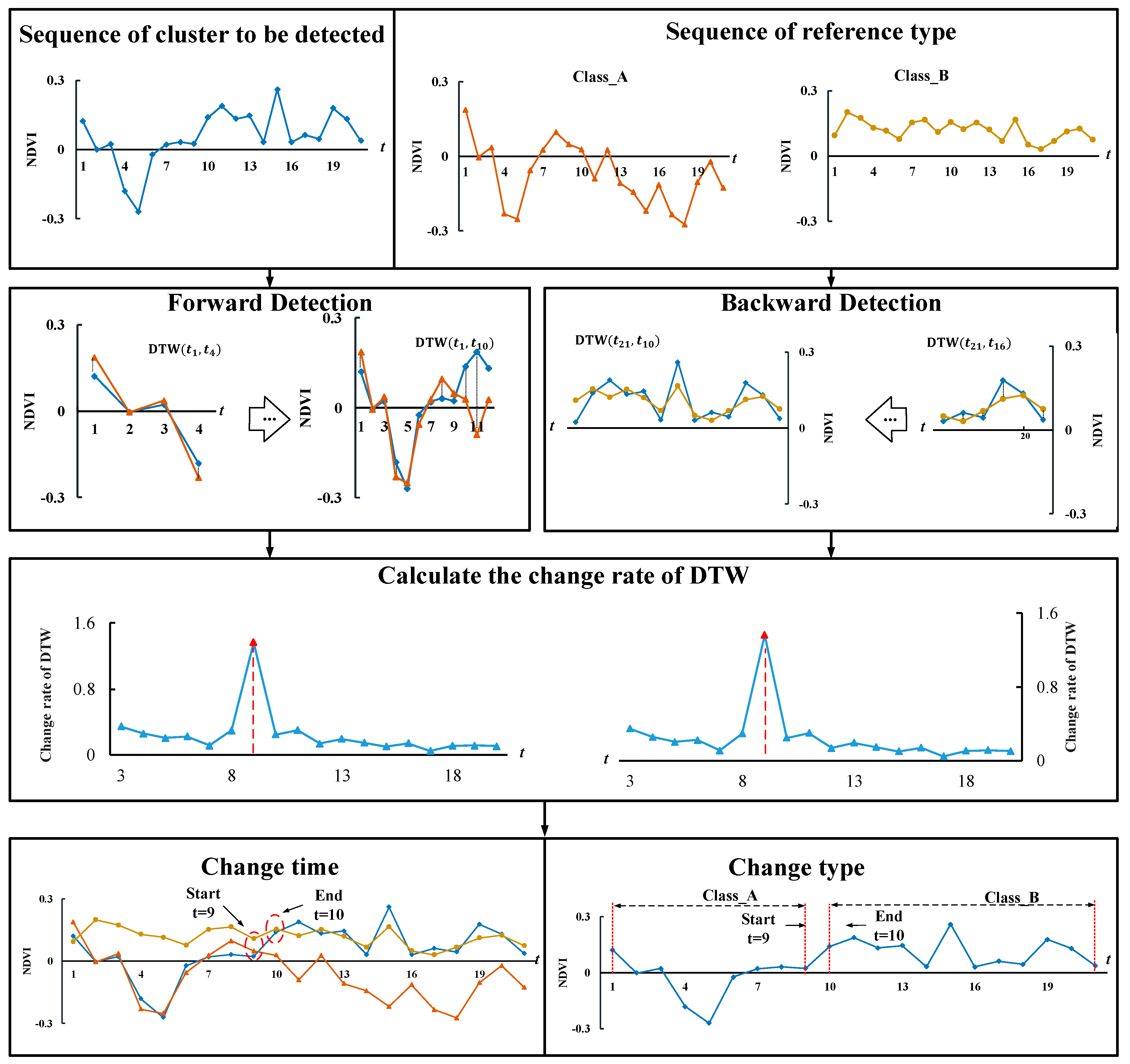
Figure 4 shows the concepts behind the BSD method. In this example, the land use of the object pending detection changed from Type A to B. In this process, its NDVI also changed, with the NDVI TS containing 21 phases. For Phases 1–9, the NDVI TS curve of the object was similar to Type A, then trended toward Type B for Phases 9–10, and became similar to Type B after Phase 10 without any reversal to Type A. The changing trend of the curve indicates that the object underwent a transition in land use from Type A to B. During the process of change, the rate of change in similarity, which was measured using the DTW distance, increased sharply. It is assumed that the phase of the most abrupt change corresponds to the point at which change occurred. Then, the TS prior to this change, the pre-change TS segment, was extracted. This segment was compared to the TS curve of each of the unchanged samples during the corresponding phase interval. During the comparison, the 3D DTW distance was used to determine similarity [12]. Thus, the type of land use before the change was determined in terms of the type of sample with the highest similarity. Similarly, the new types of land use were determined by comparing the TS curve after change to that of samples with unchanged land uses.
3.4.2. Change Detection Using the BSD Method
The BSD steps are further outlined as follows:
a. Screening of similar land use types
Assume that there are M curves to be detected, N sample curves, and that the series length for both is S. For each TS curve to be detected, mi (i = 1, 2, …, M) comparisons are made between every subset of TS, starting from the first phase and ending in the middle or end phase, and the corresponding interval of each sample curve. The DTW distance for each comparison is then separately calculated and recorded. The cumulative distance Dn (n = 1, 2, …, N) is obtained as shown in Equation (4).
where i represents the ith phase, which denotes the end of the TS subset, S is the last phase, and is the distance between the two subsequences corresponding to the first time phase and the ith time phase.
Then, the kth (1 ≤ k ≤ N) sample curve for which Dk is minimum can be identified to be most similar to the TS curve pending detection. The two land uses involved in the change, which are yet to be determined, can be identified via forward and backward detection, as described below.
b. Forward detection
The following equation is used to calculate , which is the rate of change of the DTW distance:
where . The maximum value of corresponds to the phase or point of abrupt change, which is the time at which the change in land use begins. This phase is considered the segmentation point, and the curve of the TS prior to this point is extracted as the pre-change TS segment. This segment is then compared to the corresponding TS segment of the samples to determine the type of land use before change.
c. Backward detection
Backward detection starts from the end of the TS; the search is performed in reverse toward the segmentation point detected during forward detection. Based on the rate of change in the DTW distance, the phase or point in time at which the change in land use occurs is detected. The subset of the TS between the end of the phase of change and the last phase is extracted as the TS segment after change. Then, this segment is compared to the corresponding TS segment of the samples to identify the new type of land use.
d. Accuracy evaluation
The aforementioned BSD method was used to detect the types and times of land use change. Then, the detection results were converted into vector data for precision verification. Validation points were selected to calculate the confusion matrix and evaluate the accuracy of the detection results.
Because of the low time resolution of the land use data and Google Earth images, accurate time verification could not be achieved. Therefore, this study reclassified the change time as four layers: unchanged, 2015, 2016, and 2017. By using the random sampling method [66], samples were extracted from the changed layer and from the unchanged layer. As our evaluation focused on the accuracy evaluation of a binary classification problem (changed or unchanged), this sample selection strategy could effectively reduce or even eliminate the impact of errors caused by ground reference data [67]. The two phases of land use data were intersected and analyzed to generate validation layers. The sample points were verified by combining the validation layer with a high-spatial-resolution Google Earth image.
4. Results
4.1. TS Characteristics of Various Land Use Types
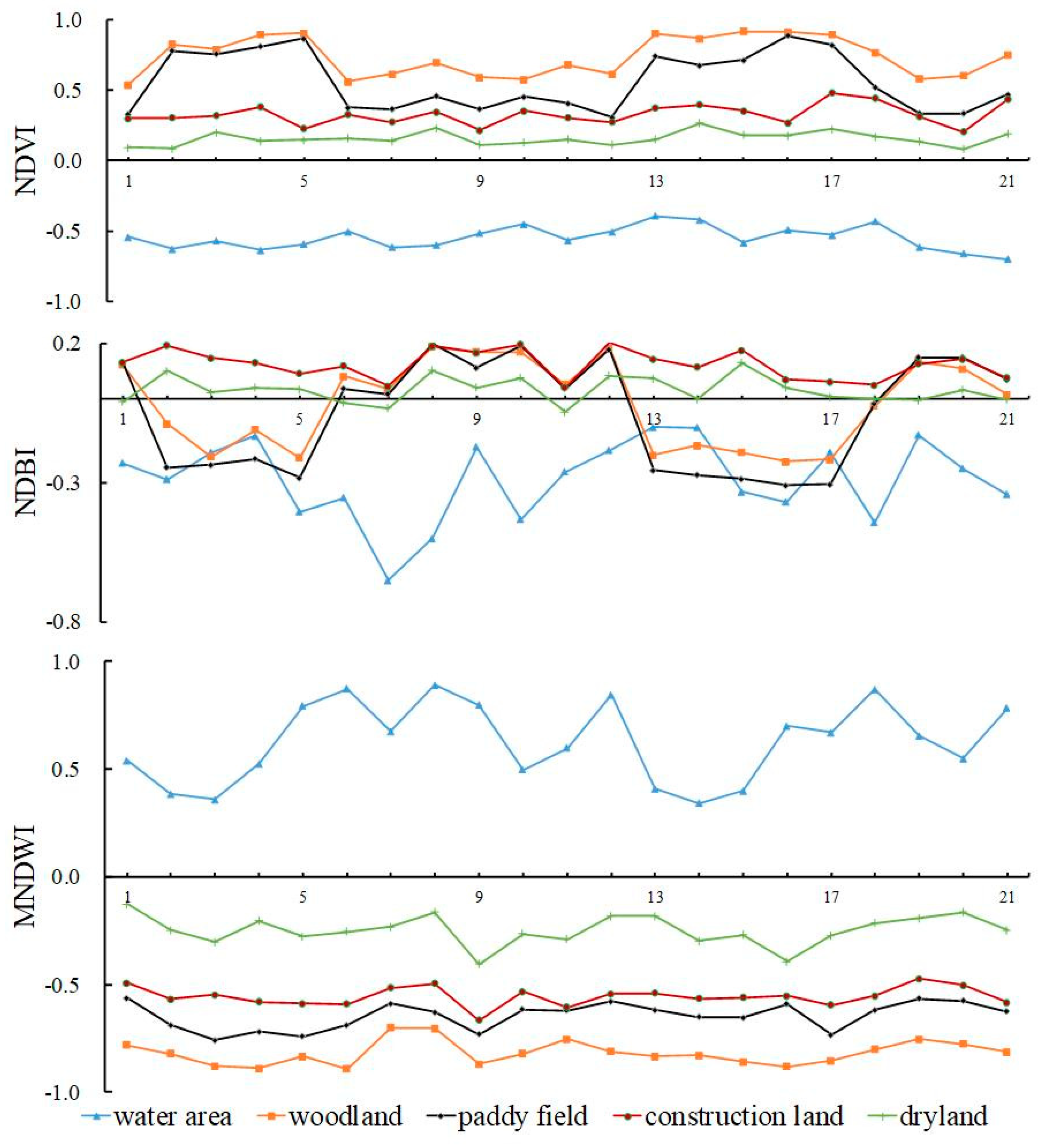
Landsat satellite images of the Xinbei District (2015–2017) and two phases of the area’s existing land use maps (2015, 2016) were used to select the TS curves of areas with unchanged land use. First, the land use maps of the two phases were superimposed for analysis. Next, Google Earth historical images were referred to and comparisons were made with the boundaries of the object after multiresolution segmentation. The sample objects for which land use had not changed were selected. Random sampling was adopted to extract 50 samples objects from each of the five types of land use (water area, woodland, paddy field, construction land, and dry land) and the mean value was calculated to form the final sample sequence data. Lastly, the NDVI, NDBI, and MNDWI TS of the sample objects of the land use types were constructed (Figure 5).
Of these indices, MNDWI was the best for distinguishing the different types of land use, followed by NDVI, and then NDBI. For all three TSs, the water areas were highly distinguishable from the other types of land use. Paddy fields and woodlands appeared to be similar in the NDVI and NDBI TSs, but they could be better distinguished in the MNDWI TS. The distinction between paddy fields and construction land in the MNDWI TS was not obvious, but clearer patterns of periodic change for paddy fields were evident in the NDVI TS. Therefore, the NDVI TS could be used to effectively distinguish paddy fields from construction lands. Moreover, the partial segments of the TS for paddy fields, woodland, and construction lands were highly similar. Thus, sufficient phases and the high time resolution of the TS played important roles in accurately distinguishing between various land uses.
4.2. Accuracy Evaluation of Land Use Change Detection
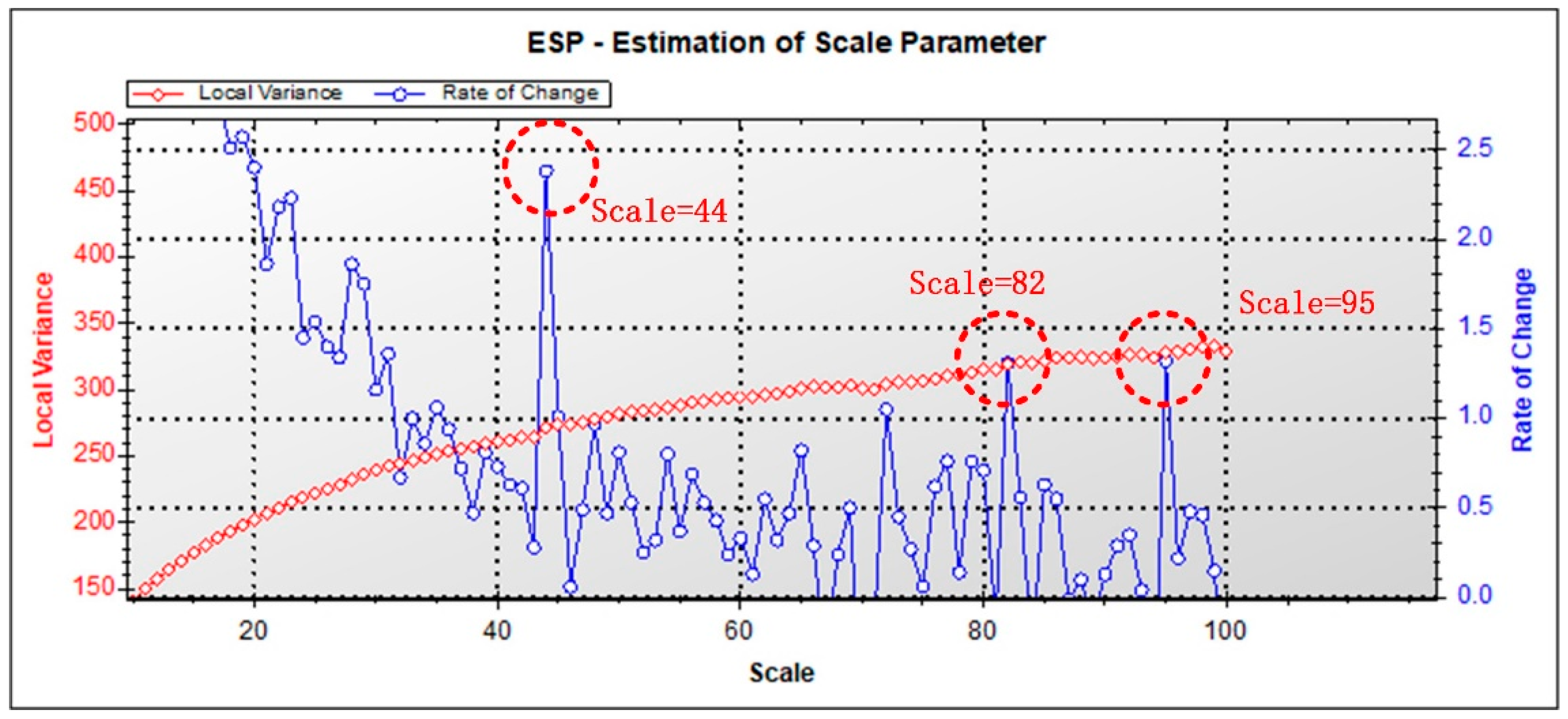
The segment parameters were as follows: maximum-scale = 100, shape = 0.2, compactness = 0.5, and weight of multispectral band = 1. Figure 6 shows the resultant ESP curve.
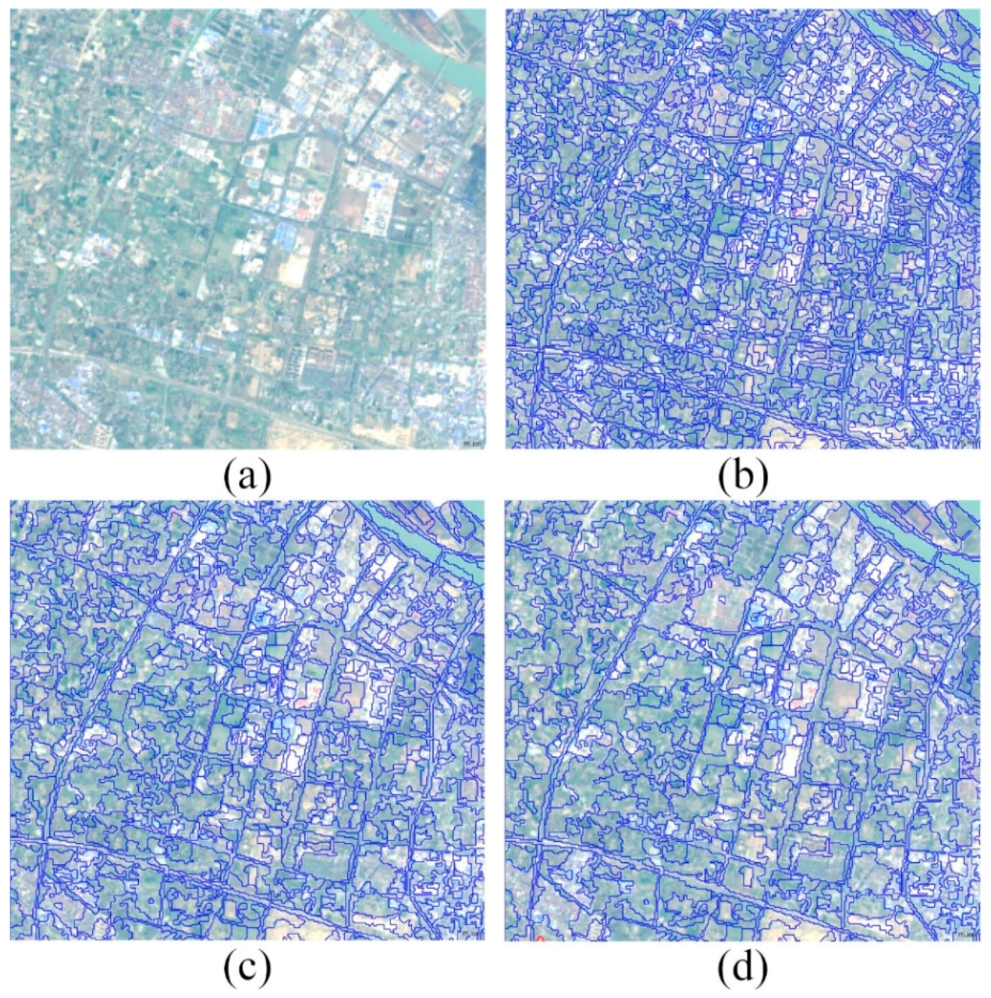
As small-scale (scale < 30) segmentation can cause object fragmentation in Landsat images, it was not considered in this study. When the segmentation scales were 44, 82, and 95, the local variance of the image’s object reached the local maxima. The curve of the change rate showed that the local variance began decreasing after the local maxima. This result indicates that the heterogeneity of the image’s object reached a maximum before decreasing. The segmentation results shown in Figure 7a–d imply that when the segmentation scale is 95, although the edges of many feature objects are intact, the phenomenon of segmented objects is significant; in other words, different ground classes appear in the same object. The segmentation effect with a scale of 82 is better than that with a scale of 95, and segmented objects still exist. In the segmentation effect results with a scale of 44, although some segmented objects exist, most of them are attributed to oversegmentation. As oversegmentation does not have an adverse impact on the detection results, 44 is the optimal scale in terms of both calculation efficiency and object accuracy. Therefore, the optimal segmentation parameters were selected as follows: segmentation scale of 44, shape factor of 0.2, compactness factor of 0.5, and all bands with a weight of one (Table 4).
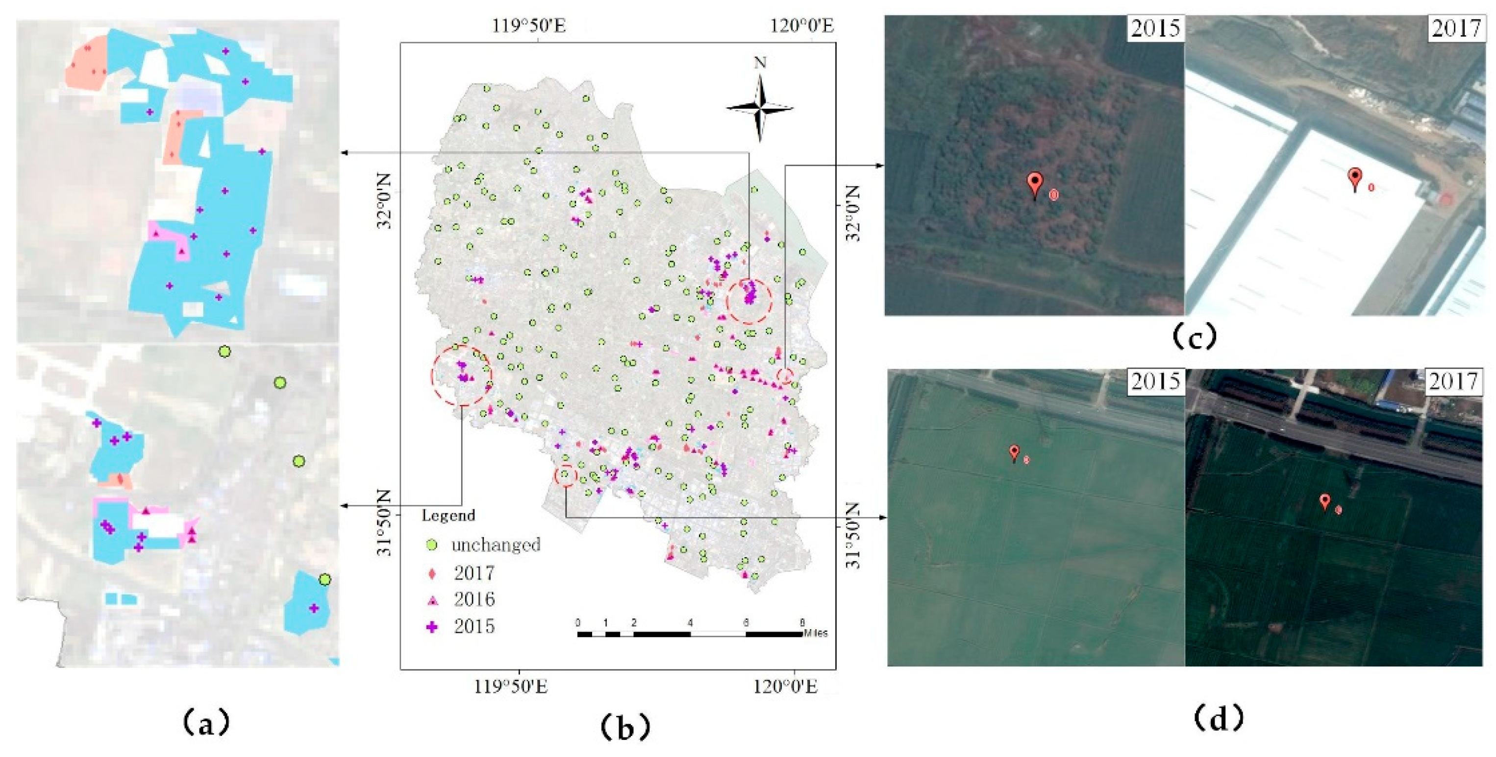
The time span of detection ranges from 7 February 2015 to 7 March 2017. The time of detection was changed on 2 August 2015, 25 October 2015, and 16 May 2016. On 28 August 2017 and 12 February 2017, 210 samples (70 samples per year) were extracted from the changed layer and another 200 samples, from the unchanged layer (Figure 8).
The detection results calculated using the confusion matrix had an overall accuracy of 90.49% and a Kappa coefficient of 0.86 (Table 5). The user and producer accuracy both exceeded 80%, where the lowest accuracy for producers occurred in 2016 and for users, in 2015. Misdetection primarily occurred in adjacent years, which may be caused by policy planning and engineering implementation not being synchronized. If only the spatial accuracy is considered and after verifying whether the detection results have changed or not considering the change time, the overall accuracy is 94.88% and Kappa coefficient is 0.89. Overall, the accuracy verification confirms that our method can achieve superior results in land use change detection compared to traditional methods.
4.3. Spatiotemporal Characteristics of Land Use Change
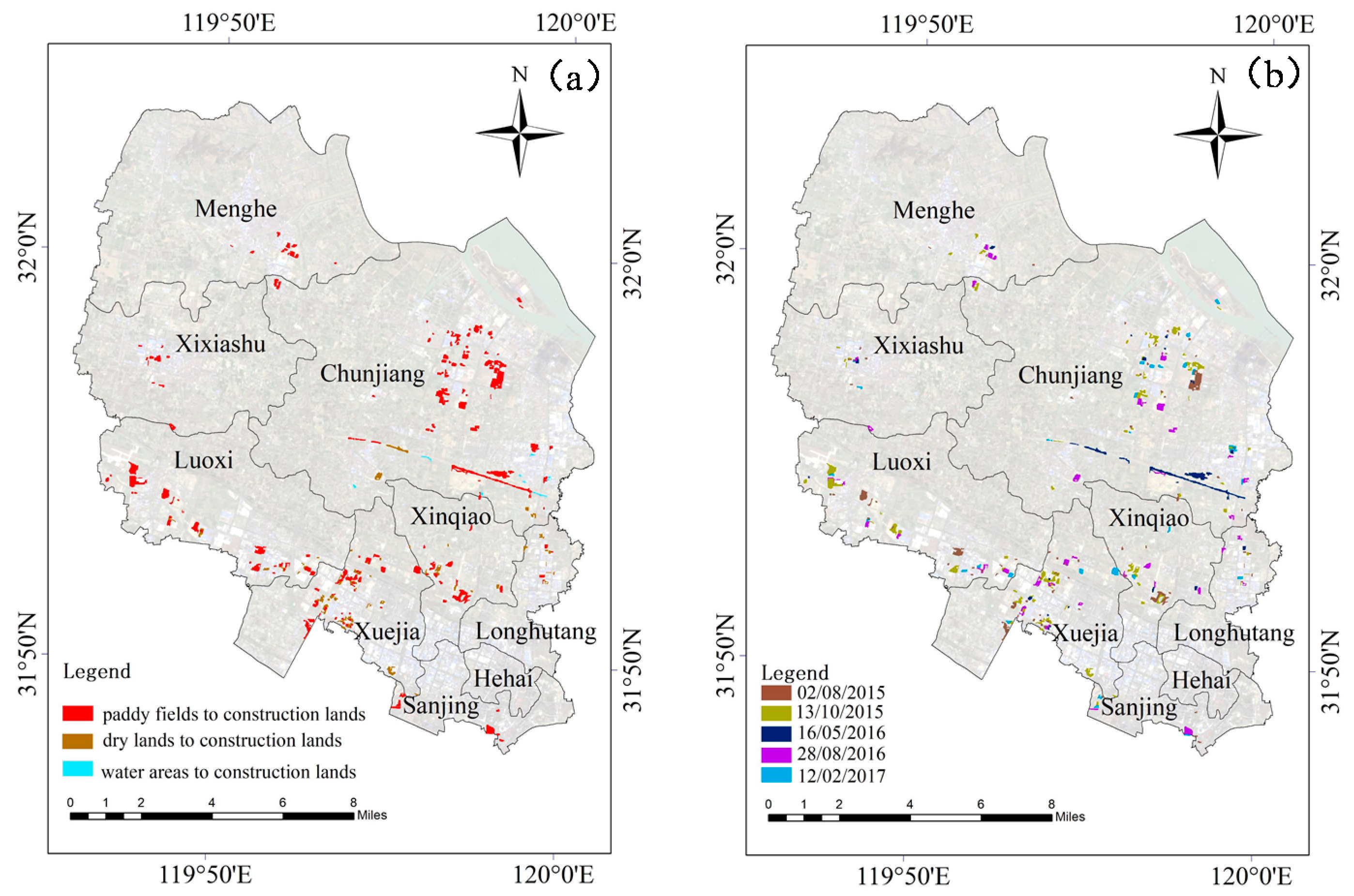
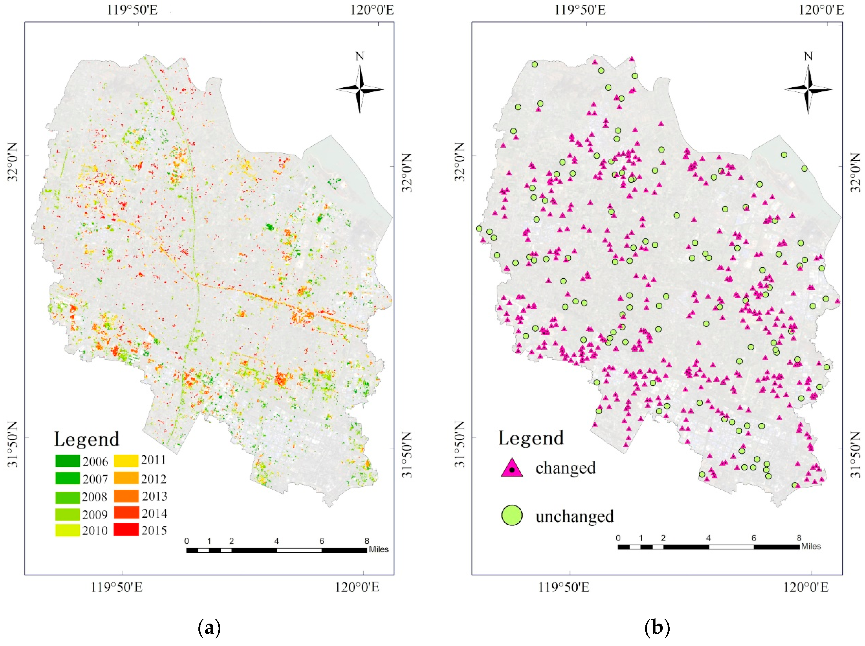
The proposed BSD method identified not only the type of change but also the time when change began. The spatial distributions of the types and times of land use change are shown in Figure 9a,b, respectively.
In terms of spatial distribution, there was a certain correlation in the regions of change. There were clusters of land use change at the centers of cities and towns or close to them. The proximity effect was observed in local areas and mainly concentrated in the towns of Chunjiang, Xuejia, and Luoxi. Chunjiang is the largest township by area in the Xinbei District. It is located on the south side of the Yangtze River and has well-developed water and land transportation systems as well as an economic development zone where several large enterprise groups and many promising industrial companies are located. Consequently, there has been rapid land use change in Chunjiang Town, wherein many paddy fields have been converted into construction lands.
Luoxi town is located adjacent to the international airport of Changzhou (Benniu Airport). It has many highways and provincial roads passing through it. It also has the largest inland river harbor in Jiangsu province, Benniu Harbor. The town has convenient air, water, land, and rail transportation facilities. Recently, many of the surrounding paddy fields and drylands have been converted for the expansion of the Benniu Airport. Xuejia town is adjacent to the northern central business district (CBD) of Changzhou, which has led to rapid conversion of paddy fields and drylands into construction land. In general, land use change is more prominent in Xinbei District because of the rapid development of the economy and transportation systems.
The changes were mainly concentrated in the summer and fall (02/08/2015, 13/10/2015, 16/05/2016, 28/08/2016), accounting for 89.66% of the total land use change. There were fewer areas with changes in winter (12/02/2017), which can be attributed to bad weather and frequent holidays (i.e., New Year’s Day and the Spring Festival), which severely affect construction efficiency. Another possible reason for this is that state approval for construction land is usually granted in the second half of the year, and construction often begins after the Spring Festival, which is usually in February. Therefore, most of the change in land use from nonconstruction to construction land occurred in the spring, summer, and fall.
The major type of land use change from February 2015 to March 2017 involved paddy fields being converted to construction land; this accounted for 73.15% of the total area changed. This was because the original land use in the Xinbei District was predominantly paddy fields. In 2016, paddy fields covered 28.62% of the total area. The paddy fields were mostly distributed in western Chunjiang Town, Xinqiao Town, and Menghe Town. However, the paddy fields converted to construction lands were mainly distributed in Luoxi Town, Xuejia Town, and the central and eastern parts of Chunjiang Town. This indicates that economic development was the main cause of land use change. Other than paddy fields, some dry lands and water areas in Xuejia and Chunjiang Town were also converted to construction land. As the patches of dry land in the Xinbei District were small and scattered near the fringes of the cities, they were less affected by the expansion of construction land.
4.4. Comparative Experiments
4.4.1. Comparisons with Results of LandTrendr Algorithm
According to the analysis of detection results, the primary land use change type is characterized by the conversion of other land use types to the construction land use type. To further study the expansion of construction land in the study area, the LandTrendr algorithm is used. The LandTrendr algorithm has provided accurate results when it has been used to detect forest disturbances, farming abandonment in agricultural land, and the disturbance-recovery of open-pit mines [41]. Wang et al. used the LandTrendr algorithm to study urban impervious surface expansion and achieved ideal results [68]. Therefore, the results of the LandTrendr algorithm were compared with those of our method to verify its suitability.
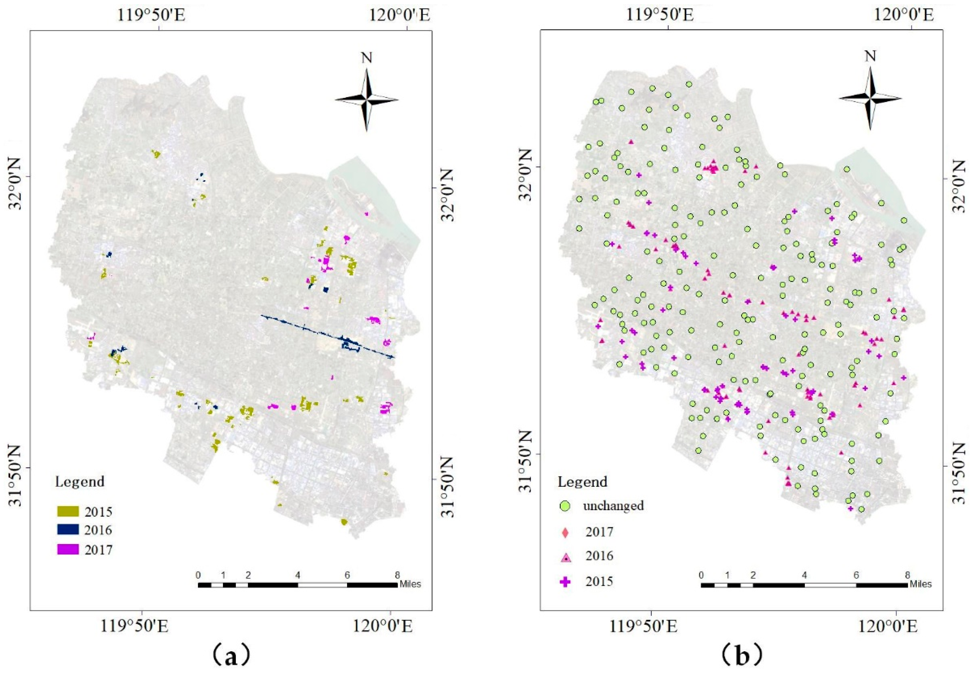
The LandTrendr algorithm can be divided into the following steps. From the TS trajectory parameters calculated by LandTrendr, the ratio of maximum disturbance value, maximum recovery value, disturbance value, and recovery value was selected as the feature. The sample of construction land expansion was obtained by using the land use change data from 2015, 2016, and 2017; the object with a trajectory of construction land expansion was extracted via a support vector machine. Figure 10 shows the extraction results. The same strategy as detailed in Section 4.2 was used to evaluate the accuracy; Table 6 shows the resulting confusion matrix.
As shown in Figure 10a, the BSD results are highly consistent with those of LandTrendr, such that the regions with significant changes are accurately extracted. BSD is less effective than LandTrendr in road detection. In terms of detection accuracy, the overall accuracy of LandTrendr is 84.39%; however, the perception of changing years is not as sensitive as in the BSD method, that is, there are more misclassifications in adjacent years.
4.4.2. Comparison with Change Detection Methods Based on TS Similarity
Traditional methods of identifying land use change based on TS similarity are based on the idea of supervised classification. Samples of land use change are selected before classification. Then, the similarity between the TS of objects pending detection and those of the samples is measured individually. With an appropriate distance threshold, if the similarity is less than the threshold, it is assumed that the same type of land use change has occurred for the pending objects and samples. However, it is difficult to accurately determine the time of change because the samples may not cover all the types and times of land use change, which leads to many false detections.
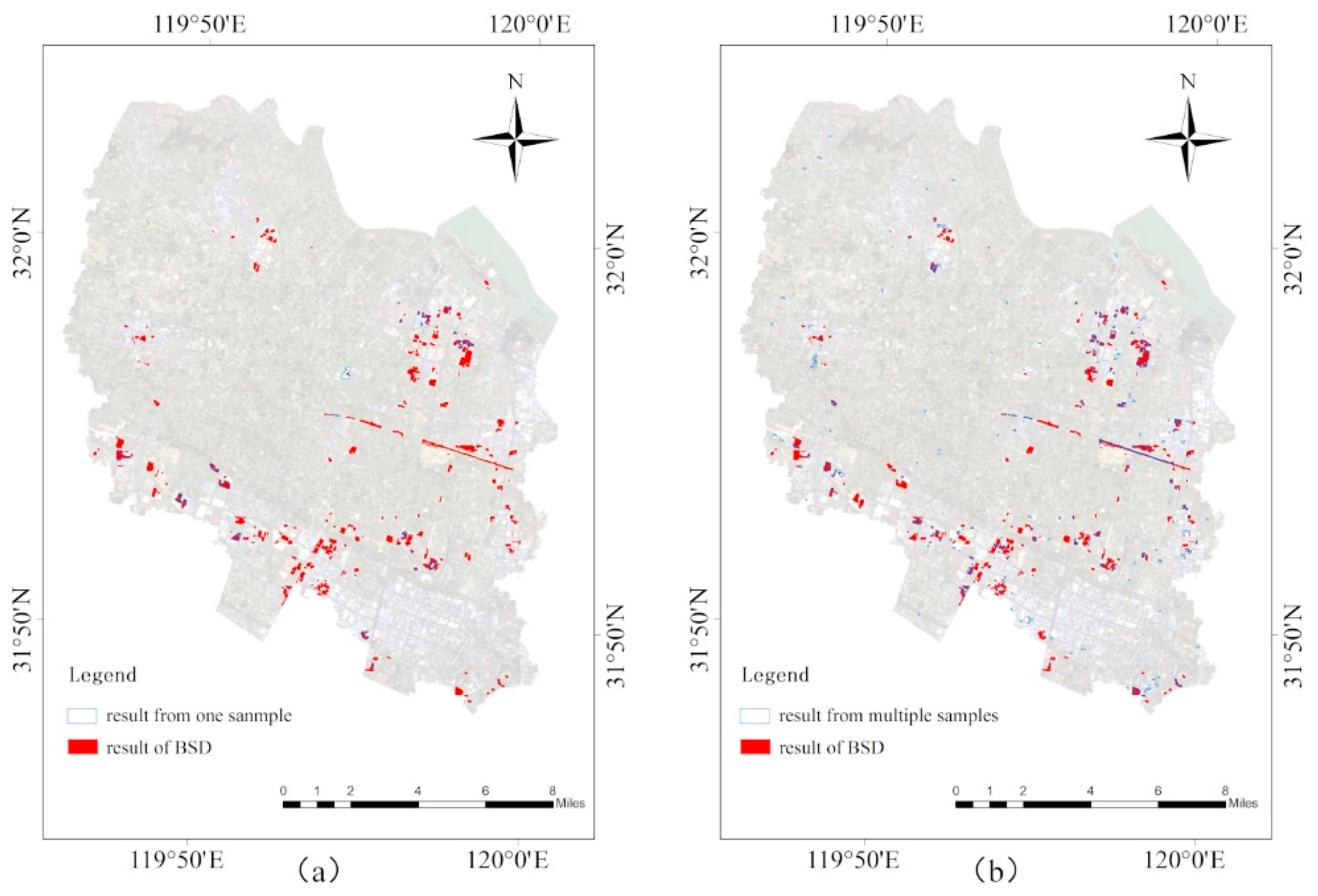
To compare the BSD method with the TS similarity method, a predominant type of land use change—conversion from paddy field to construction land—was detected using both methods. For the TS similarity method, two sample sets were used. The first set was a sample where land use changed on 13 October 2015, with most conversions involving paddy field land use to construction land use. The second set included five samples wherein land use changed on 02 August 2015, 13 October 2015, 16 May 2016, 28 August 2016, and 12 February 2017. The second set covered all change times detected, as outlined in Section 4.4. The similarity threshold used in the experiment was 2.5 (Figure 11).
Many objects where conversion from paddy field to construction land occurred were not detected using the TS similarity method with the first sample set. The second sample set was better than the first; however, it also resulted in many omission errors. The BSD method outperformed the TS similarity method for both the first and the second sample sets. Additionally, unlike in the TS similarity method, which only detected conversions from paddy fields to construction land, the BSD method also detected conversions from water areas and dry land to construction land. The BSD method avoids the issue of sample inadequacy and can thus be used to detect land use change more comprehensively.
4.4.3. Comparison with Change Detection Based on Mean TS Similarity
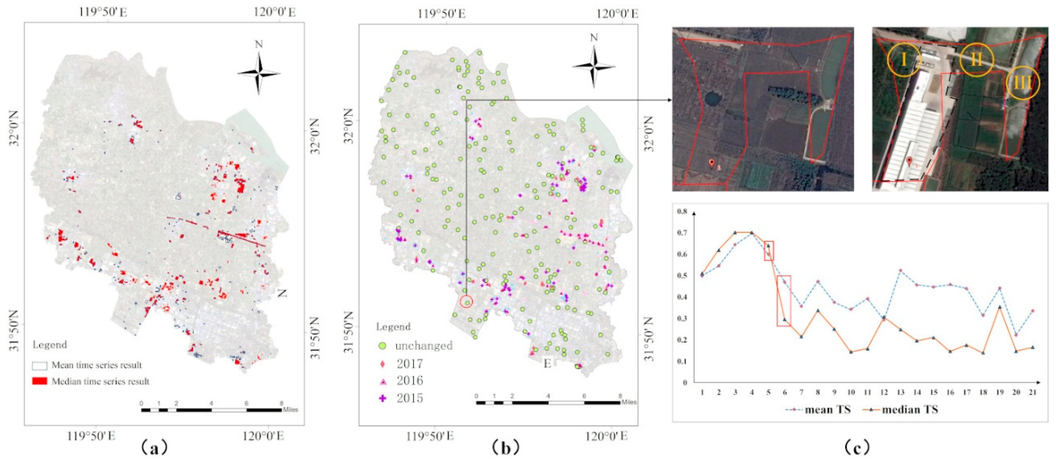
Most existing studies on object-level TS use the mean index of all pixels in an object as the representative feature. However, the median index of the pixels is more representative because it better reflects the index characteristics of the majority of the pixels in the object and reduces the influence of outliers and noise. Therefore, the median can increase the difference between land types, as shown in Figure 3. Here, we also compared the difference between these two TS approaches (Figure 12a).
Although the overall accuracy of the mean TS reached 83.17%, the producer accuracy is close to 80%, whereas the user accuracy of the changing results is less than 85% (Table 7). There are many large plots that were not successfully detected (Figure 12b). We chose a typical sample object. From Figure 12c, the part of the object that actually changed was a building contained in the dashed line; areas I, II, and III included unchanged surface features. This leads to the difference between the mean TS and the median TS curves shown in Figure 12c. It is clear that the median can better characterize change during change detection.
5. Discussion
5.1. Applicability of BSD Method and Discussion of Multiple Change Detection Method
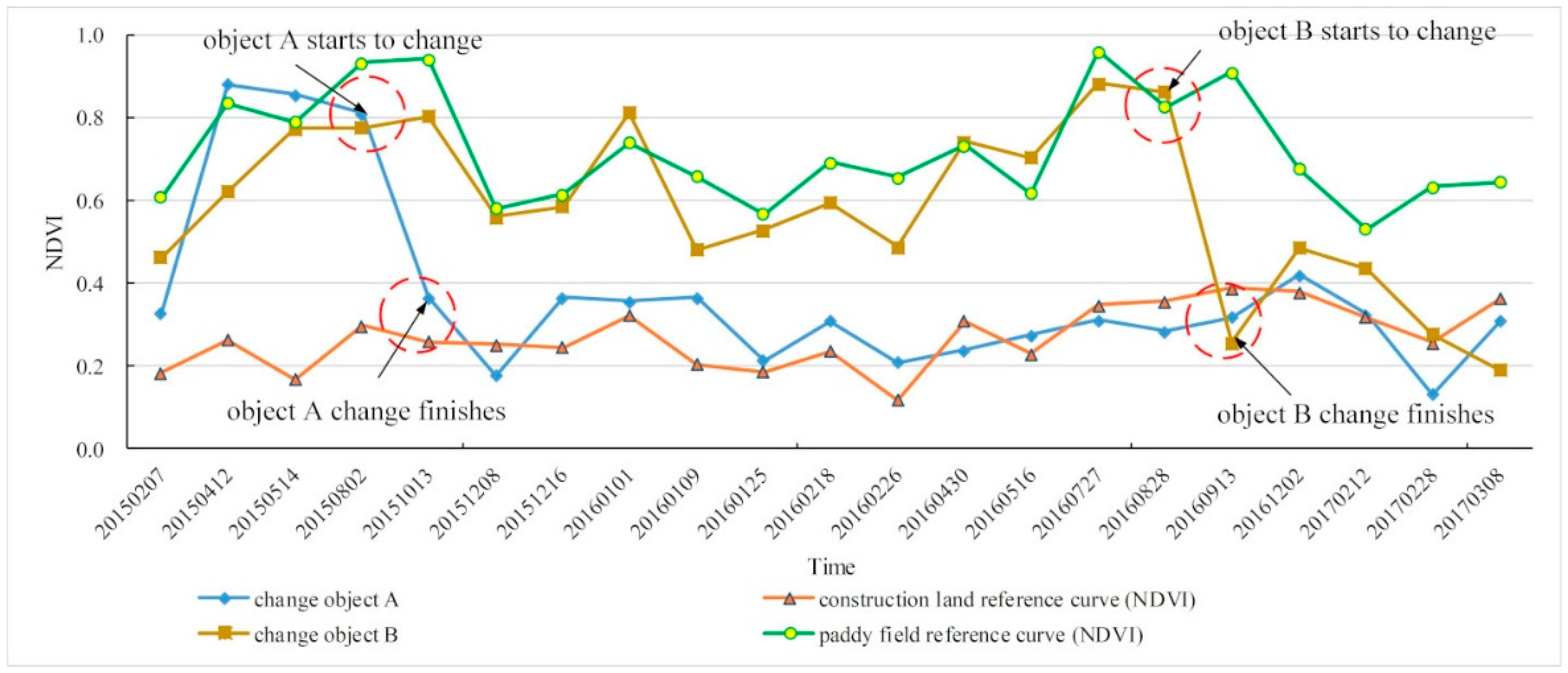
In land use change detection, the commonly used methods cannot simultaneously determine the change time and type. The BSD method proposed herein can effectively address this problem. The TS curves of objects whose land use does not change were used to identify the type and time of change in the segmented objects. This method can be applied to detect land use change for objects with similar types of change but different change times. In this study, both objects A and B underwent the same type of land use change, from paddy fields to construction land (Figure 13). However, the change time was different for each: object A’s change began on 2 August 2015, whereas object B’s change began on 28 August 2016. The proposed BSD method simply and effectively detects both the type and the time of land use change. It does not need samples of land use change for every type and time of change, and only unchanged samples are needed, which simplifies sample selection.
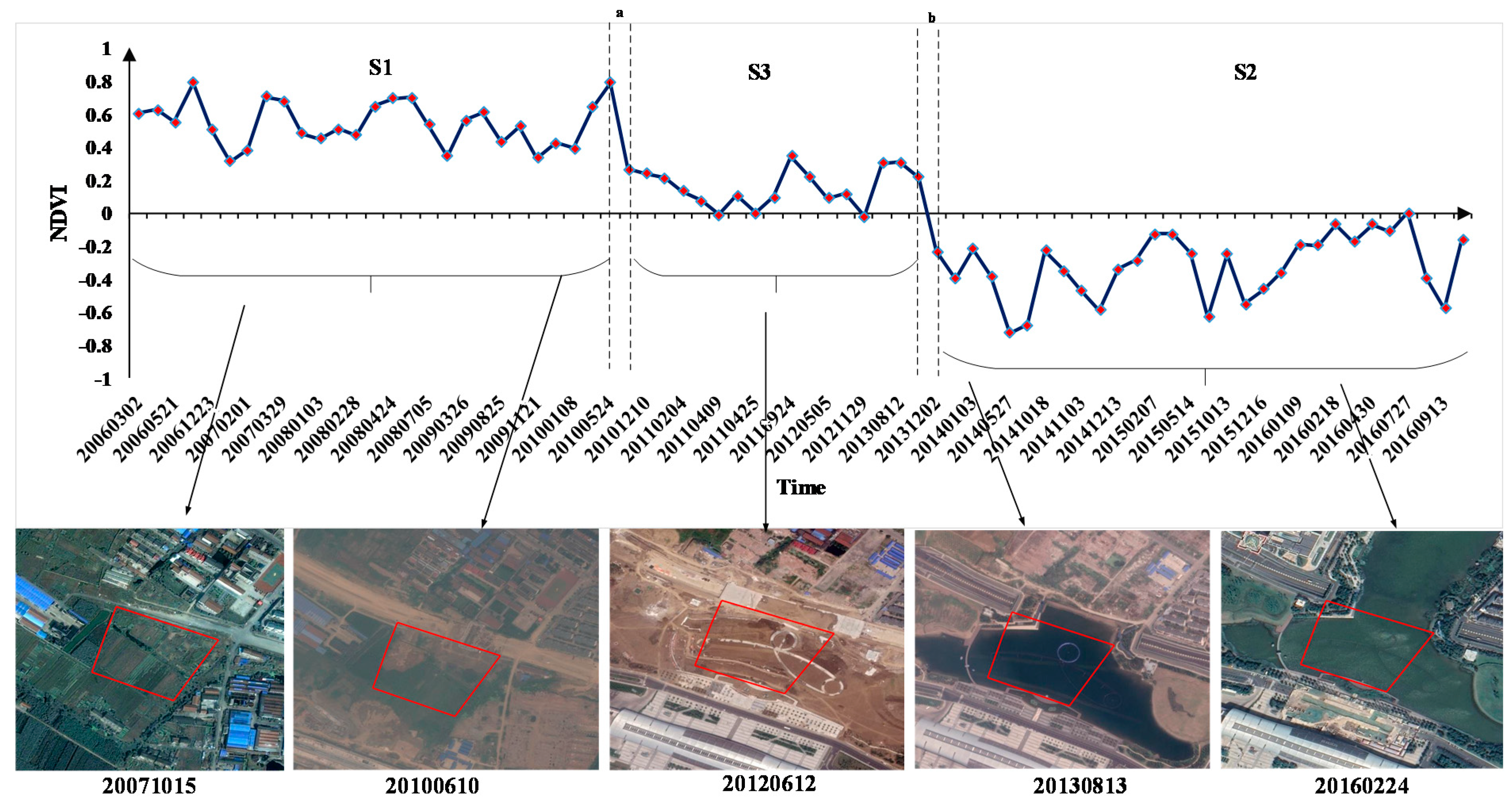
It must be noted that the proposed BSD method cannot be directly applied to areas with a long-term TS or frequent land use changes. However, it can be used if the long-term TS is divided into shorter periods. Figure 14 shows a schematic diagram of the multiple change detection method. First, we need to use the S-G algorithm to filter the long TS, and then five (or more) parts, S1, S2, S3, a, and b, are obtained using the BSD method. Here, a and b are in the change stage and S1 and S2 are respectively the start state and the final state. Next, the change process subsequence (a, b) is removed, and the BSD method is used to detect the change process of the S3 subsequence; therefore, reverse iteration occurs until all subsequences are detected. Finally, land use changes during the various periods are combined to determine the land use change in a long-term TS.
5.2. Experiment with Long TS
To test the applicability of the algorithm for a long TS, this study selects Landsat images from March to May in 2006–2016 (Table 8) and detects the expansion results of construction land in the study area in 2006–2016 using the BSD method after the S-G filter (Figure 15a). By using the confusion matrix to evaluate the accuracy and the stratified sampling method, 500 samples that change every year and 120 that remain unchanged are taken from the results, for a total of 620 sample points (Figure 15b).
Table 9 shows the confusion matrix. The overall accuracy is 89.19% and Kappa coefficient is 0.88; this demonstrates that the BSD method can well detect the expansion and change time points of construction land. Among them, five of the 120 unchanged sample points have construction land expansion in different years, whereas only 12 of the sample points have no construction land expansion. In addition, most of the error samples detected at the change time point are one year, but a few are two years. The user accuracy of the change time points in 2006, 2013, and 2015 is low, which may be due to the fact that they are at both ends of the TS, and the subsequences after segmentation are short and cannot be identified accurately.
Therefore, the BSD method proposed in this study can be applied to a long TS, and it can provide new ideas and methods for land use change detection in a large area over a long time. However, for a smaller time range and more precise land change identification, it is still unable to achieve accurate monitoring. In the future, the data and methods will be improved continuously. For example, future work will focus on accurately detecting the changing time points of long-term and multiple changing geographical elements through additional effective algorithms.
5.3. Influence of Gap-Filled Area on Change Detection
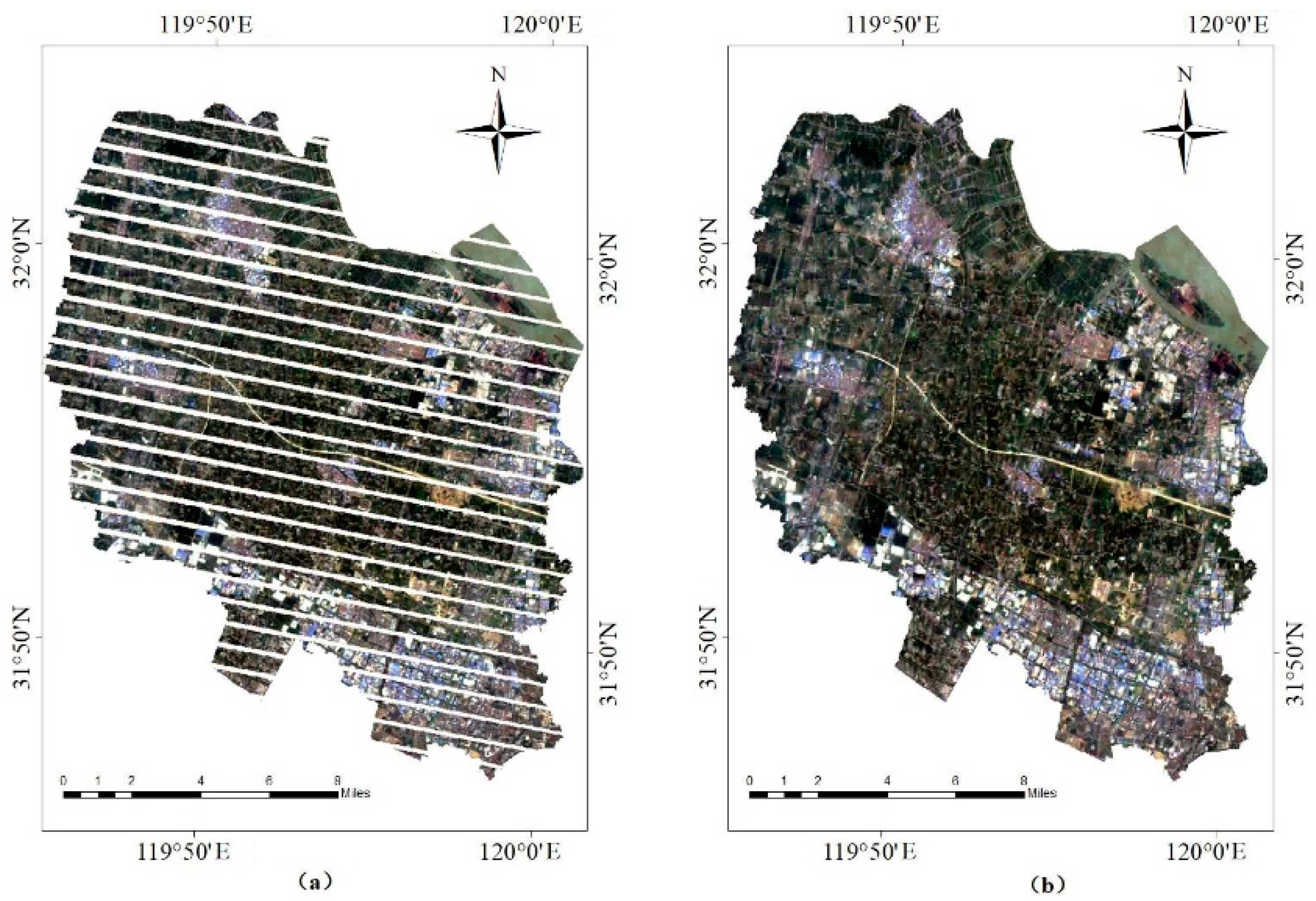
The reliability of the pixel value of the gap-filled area directly affects the accuracy of change detection. As mentioned in Section 3.2, many scholars have proved that the gap-filled image has excellent usability. Figure 16a,b show the comparison of the effect of an ETM + image in the study area before and after gap-filling on 30 April 2015. It can be seen that the visual effect after restoration is excellent.
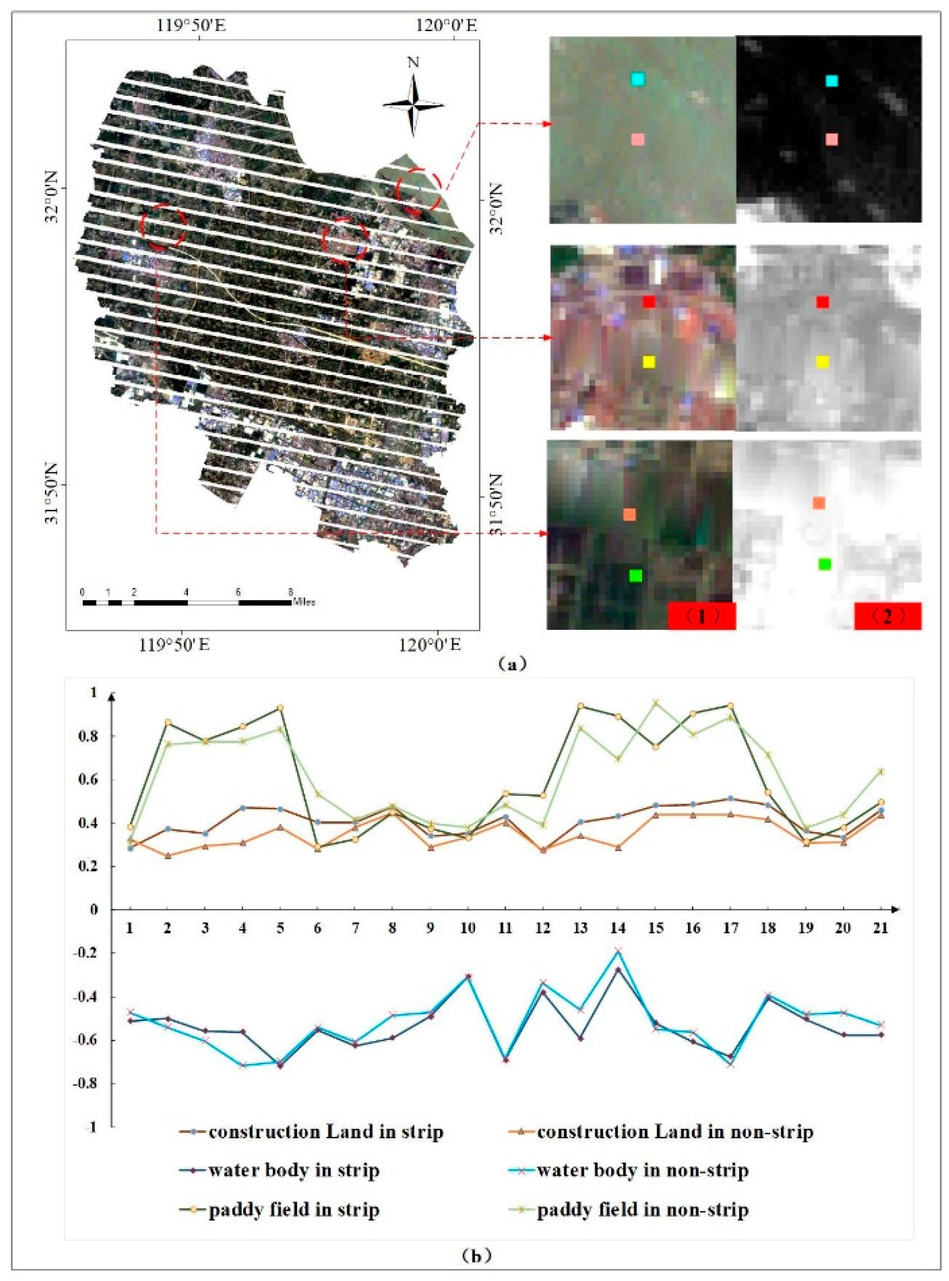
From the TS perspective, this study discussed the impact of the gap-filled ETM + image on land-cover change detection. Figure 16a,b show the images before and after filling, respectively. According to the results of land use change detection, three main sample pixels of land cover were selected (Figure 17a) and their NDVI TS data were counted. As shown in Figure 17b, the gap-filled pixel values of the water land use type are most similar to the normal pixel values for the same type. The effect of the gap-filled paddy field area is not optimal; however, the overall trend is consistent with the normal paddy field pixels. For TS-based research, as long as the trends are consistent, the gap-filled ETM + image does not have a significant impact on the results. The gap-filled value of construction land is slightly higher than the normal value of construction land; however, its sequence trend is highly consistent with that of normal pixels. In conclusion, it is feasible to apply the gap-filled Landsat ETM + images to TS studies.
6. Conclusions
This study proposed bidirectional segmented change detection based on object-level multivariate TS to detect the type and time of land use change from Landsat images. The study area was Xinbei District of Changzhou City. A total of 21 images from 2015–2017 were selected for the experiment. The main conclusions are as follows:
- The proposed BSD method can effectively detect the type and time of an object’s change. Multitemporal images were segmented and the 3D DTW method was adopted to detect the generated object and samples with unchanged land use via the BSD method. The results show that this method can be used to identify objects that have undergone land use changes with an overall accuracy of 90.49% and a Kappa coefficient of 0.86. Moreover, the method has good scalability for a long TS.
- The median index of a segmented object is more representative than the commonly used mean. Although the overall accuracy of the mean TS reached 83.17%, both the omission and the commission were approximately 15%. Objects generated via image segmentation contain clusters of similar pixels. However, differences in the index values between an object’s edge and internal pixels were especially prominent. The median index of the pixels of objects can better extract the main features of object timing and enhance the stability of timing analysis.
- In the Xinbei District from 2015–2017, the main types of land use change were the conversion of paddy fields, dry land, and water areas to construction land; the change from paddy fields to construction land accounted for 73.15% of the total area changed. In terms of spatial distribution, these changes mostly occurred in areas with rapid economic development. These changes were also near transportation hubs and in urban centers, where the demand for expansion was higher. The times of change were mainly concentrated in summer and fall.
Further study is needed on long-term TS with frequent changes in land use to improve the applicability of object-level TS analysis to complex land use change detection.
Author Contributions
All authors contributed to this work. Y.H. and Z.C. conceived the study and designed the research. Y.H. drafted the manuscript, which was revised by Q.H. and F.L. B.W. and L.M. contributed to data processing and experiments. All authors have read and agreed to the published version of the manuscript.
Funding
This work is supported by the National Key Research and Development Program of China (No. 2017YFB0504205) and the National Natural Science Foundation of China (No. 41571378, 41671386).
Acknowledgments
We thank the National Aeronautics and Space Administration and the Chinese Academy of Sciences Geospatial Data Cloud for providing free use of their Landsat satellite images.
Conflicts of Interest
The authors declare no conflict of interest.
References
- Turner, B.; Moss, R.H.; Skole, D.L. Relating Land Use and Global Land-Cover Change: A Proposal for an IGBP-HDP Core Project. Global Change Report 1993. Available online: https://bit.ly/2ScdeL6 (accessed on 31 January 2020).
- Vitousek, P.M. Beyond Global Warming: Ecology and Global Change. Ecology 1994, 75, 1861–1876. [Google Scholar] [CrossRef]
- Li, M.; Stein, A.; Bijker, W.; Zhan, Q. Urban land use extraction from Very High Resolution remote sensing imagery using a Bayesian network. ISPRS J. Photogramm. Remote. Sens. 2016, 122, 192–205. [Google Scholar] [CrossRef]
- Chen, Y.; Lu, D.; Luo, L.; Pokhrel, Y.; Deb, K.; Huang, J.; Ran, Y. Detecting irrigation extent, frequency, and timing in a heterogeneous arid agricultural region using MODIS time series, Landsat imagery, and ancillary data. Remote. Sens. Environ. 2018, 204, 197–211. [Google Scholar] [CrossRef]
- El-Asmar, H.M.; Hereher, M.E.; El Kafrawy, S.B. Surface area change detection of the Burullus Lagoon, North of the Nile Delta, Egypt, using water indices: A remote sensing approach. Egypt. J. Remote. Sens. Space Sci. 2013, 16, 119–123. [Google Scholar] [CrossRef] [Green Version]
- Hermosilla, T.; Wulder, M.A.; White, J.C.; Coops, N.C.; Hobart, G.W. An integrated Landsat time series protocol for change detection and generation of annual gap-free surface reflectance composites. Remote. Sens. Environ. 2015, 158, 220–234. [Google Scholar] [CrossRef]
- Gómez, C.; White, J.C.; Wulder, M.A. Optical remotely sensed time series data for land cover classification: A review. ISPRS J. Photogramm. Remote. Sens. 2016, 116, 55–72. [Google Scholar] [CrossRef] [Green Version]
- Long, J.A.; Lawrence, R.L.; Greenwood, M.C.; Marshall, L.; Miller, P.R. Object-oriented crop classification using multitemporal ETM+ SLC-off imagery and random forest. GISci. Remote Sens. 2013, 50, 418–436. Available online: https://bit.ly/3aZoCCI (accessed on 31 January 2020). [CrossRef]
- Zhu, Z.; Woodcock, C.E. Continuous change detection and classification of land cover using all available Landsat data. Remote. Sens. Environ. 2014, 144, 152–171. [Google Scholar] [CrossRef] [Green Version]
- Zhu, Z.; Zhang, J.; Yang, Z.; Aljaddani, A.H.; Cohen, W.B.; Qiu, S.; Zhou, C. Continuous monitoring of land disturbance based on Landsat time series. Remote. Sens. Environ. 2019, 111116. [Google Scholar] [CrossRef]
- Cheng, L.; Wang, Y.; Li, M.; Zhong, L.; Wang, J. Generation of Pixel-Level SAR Image Time Series Using a Locally Adaptive Matching Technique. Photogram. Eng. Remote Sens. 2014, 80, 839–848. [Google Scholar] [CrossRef]
- Wang, W.; Chen, Z.; Li, X.; Tang, H.; Huang, Q.; Qu, L. Detecting spatio-temporal and typological changes in land use from Landsat image time series. J. Appl. Remote Sens. 2017, 11, 035006. [Google Scholar] [CrossRef]
- Shang, R.; Liu, R.; Xu, M.; Liu, Y.; Zuo, L.; Ge, Q. The relationship between threshold-based and inflexion-based approaches for extraction of land surface phenology. Remote Sens. Environ. 2017, 199, 167–170. [Google Scholar] [CrossRef]
- Ney, H.; Ortmanns, S. Dynamic programming search for continuous speech recognition. IEEE Signal Process. Mag. 1999, 16, 64–83. [Google Scholar] [CrossRef] [Green Version]
- Petitjean, F.; Inglada, J.; Gancarski, P. Satellite Image Time Series Analysis Under Time Warping. IEEE Trans. Geosci. Remote Sens. 2012, 50, 3081–3095. [Google Scholar] [CrossRef]
- Keogh, E.; Ratanamahatana, C.A. Exact indexing of dynamic time warping. Knowl. Inf. Syst. 2005, 7, 358–386. [Google Scholar] [CrossRef]
- Chen, Y.-L.; Wu, S.-Y.; Wang, Y.-C. Discovering multi-label temporal patterns in sequence databases. Inf. Sci. 2011, 181, 398–418. [Google Scholar] [CrossRef]
- Lee, A.J.T.; Chen, Y.-A.; Ip, W.-C. Mining frequent trajectory patterns in spatial–temporal databases. Inf. Sci. 2009, 179, 2218–2231. [Google Scholar] [CrossRef]
- Guan, X.; Huang, C.; Liu, G.; Meng, X.; Liu, Q. Mapping Rice Cropping Systems in Vietnam Using an NDVI-Based Time-Series Similarity Measurement Based on DTW Distance. Remote Sens. 2016, 8, 19. [Google Scholar] [CrossRef] [Green Version]
- Petitjean, F.; Weber, J. Efficient Satellite Image Time Series Analysis Under Time Warping. IEEE Geosci. Remote Sens. Lett. 2014, 11, 1143–1147. [Google Scholar] [CrossRef]
- Yan, J.; Wang, L.; Song, W.; Chen, Y.; Chen, X.; Deng, Z. A time-series classification approach based on change detection for rapid land cover mapping. ISPRS-J. Photogramm. Remote Sens. 2019, 158, 249–262. [Google Scholar] [CrossRef]
- Jeong, Y.-S.; Jeong, M.K.; Omitaomu, O.A. Weighted dynamic time warping for time series classification. Pattern Recognit. 2011, 44, 2231–2240. [Google Scholar] [CrossRef]
- Nasrallah, A.; Baghdadi, N.; Mhawej, M.; Faour, G.; Darwish, T.; Belhouchette, H.; Darwich, S. A Novel Approach for Mapping Wheat Areas Using High Resolution Sentinel-2 Images. Sensors 2018, 18, 2089. [Google Scholar] [CrossRef] [PubMed] [Green Version]
- Maus, V.; Câmara, G.; Cartaxo, R.; Sanchez, A.; Ramos, F.M.; de Queiroz, G.R. A Time-Weighted Dynamic Time Warping Method for Land-Use and Land-Cover Mapping. IEEE J. Sel. Top. Appl. Earth Observ. Remote Sens. 2016, 9, 3729–3739. [Google Scholar] [CrossRef]
- Faour, G.; Mhawej, M.; Nasrallah, A. Global trends analysis of the main vegetation types throughout the past four decades. Appl. Geogr. 2018, 97, 184–195. [Google Scholar] [CrossRef]
- Bovolo, F.; Bruzzone, L. A Theoretical Framework for Unsupervised Change Detection Based on Change Vector Analysis in the Polar Domain. IEEE Trans. Geosci. Remote Sens. 2007, 45, 218–236. [Google Scholar] [CrossRef] [Green Version]
- Nemmour, H.; Chibani, Y. Multiple support vector machines for land cover change detection: An application for mapping urban extensions. ISPRS-J. Photogramm. Remote Sens. 2006, 61, 125–133. [Google Scholar] [CrossRef]
- Castillejo-González, I.L.; López-Granados, F.; García-Ferrer, A.; Peña-Barragán, J.M.; Jurado-Expósito, M.; de la Orden, M.S.; González-Audicana, M. Object- and pixel-based analysis for mapping crops and their agro-environmental associated measures using QuickBird imagery. Comput. Electron. Agric. 2009, 68, 207–215. [Google Scholar] [CrossRef]
- Ma, L.; Li, M.; Ma, X.; Cheng, L.; Du, P.; Liu, Y. A review of supervised object-based land-cover image classification. ISPRS-J. Photogramm. Remote Sens. 2017, 130, 277–293. [Google Scholar] [CrossRef]
- Wang, R.S.M.; Efford, N.D.; Roberts, S.A. Object-Based Approach to Integrate Remotely Sensed Data within a GIS Context for Land Use Changes Detection at Urban-Rural Fringe Areas; Cecchi, G., Engman, E.T., Zilioli, E., Eds.; SPIE: London, UK, 1997; pp. 362–370. [Google Scholar]
- Blaschke, T.; Burnett, C.; Pekkarinen, A. New contextual approaches using image segmentation for object-based classification. In Proceedings of the Remote Sensing Image Analysis: Including the Spatial Domain; Kluwer Academic Publishersa: Dordrecht, The Netherlands; Aamsterdam, The Netherlands, 2004; pp. 211–236. [Google Scholar]
- Bayramov, E.; Buchroithner, M.; Bayramov, R. Quantitative assessment of 2014–2015 land-cover changes in Azerbaijan using object-based classification of LANDSAT-8 timeseries. Model. Earth Syst. Environ. 2016, 2, 35. [Google Scholar] [CrossRef] [Green Version]
- Matton, N.; Canto, G.; Waldner, F.; Valero, S.; Morin, D.; Inglada, J.; Arias, M.; Bontemps, S.; Koetz, B.; Defourny, P. An Automated Method for Annual Cropland Mapping along the Season for Various Globally-Distributed Agrosystems Using High Spatial and Temporal Resolution Time Series. Remote Sens. 2015, 7, 13208–13232. [Google Scholar] [CrossRef] [Green Version]
- Peña-Barragán, J.M.; Ngugi, M.K.; Plant, R.E.; Six, J. Object-based crop identification using multiple vegetation indices, textural features and crop phenology. Remote Sens. Environ. 2011, 115, 1301–1316. [Google Scholar] [CrossRef]
- Zhao, M.; Zhao, Y.D. Object-oriented and multi-feature hierarchical change detection based on CVA for high-resolution remote sensing imagery. J. Remote Sens. 2018, 22, 119–131. [Google Scholar]
- Desclée, B.; Bogaert, P.; Defourny, P. Forest change detection by statistical object-based method. Remote Sens. Environ. 2006, 102, 1–11. [Google Scholar] [CrossRef]
- Whelen, T.; Siqueira, P. Use of time-series L-band UAVSAR data for the classification of agricultural fields in the San Joaquin Valley. Remote Sens. Environ. 2017, 193, 216–224. [Google Scholar] [CrossRef]
- Bontemps, S.; Bogaert, P.; Titeux, N.; Defourny, P. An object-based change detection method accounting for temporal dependences in time series with medium to coarse spatial resolution. Remote Sens. Environ. 2008, 112, 3181–3191. [Google Scholar] [CrossRef]
- Petitjean, F.; Kurtz, C.; Passat, N.; Gançarski, P. Spatio-temporal reasoning for the classification of satellite image time series. Pattern Recognit. Lett. 2012, 33, 1805–1815. [Google Scholar] [CrossRef] [Green Version]
- Masek, J.G.; Vermote, E.F.; Saleous, N.E.; Wolfe, R.; Lim, T.K. A Landsat Surface Reflectance Data Set for North America, 1990–2000. IEEE Geosci. Remote Sens. Lett. 2006, 3, 68–72. [Google Scholar]
- Yin, H.; Prishchepov, A.V.; Kuemmerle, T.; Bleyhl, B.; Buchner, J.; Radeloff, V.C. Mapping agricultural land abandonment from spatial and temporal segmentation of Landsat time series. Remote Sens. Environ. 2018, 210, 12–24. [Google Scholar] [CrossRef]
- Pat Scaramuzza; Esad Micijevic; Gyanesh Chander SLC Gap-Filled Products Phase One Methodology. Available online: http://landsat.usgs.gov/documents/SLC_Gap_Fill_Methodology.pdf. (accessed on 20 June 2012).
- Mozumder, C.; Reddy, K.V.; Pratap, D. Air Pollution Modeling from Remotely Sensed Data Using Regression Techniques. J. Indian Soc. Remote Sens. 2013, 41, 269–277. [Google Scholar] [CrossRef]
- Vlassova, L.; Pérez-Cabello, F. Effects of post-fire wood management strategies on vegetation recovery and land surface temperature (LST) estimated from Landsat images. Int. J. Appl. Earth Obs. Geoinf. 2016, 44, 171–183. [Google Scholar] [CrossRef]
- Romero-Sanchez, M.E.; Ponce-Hernandez, R.; Franklin, S.E.; Aguirre-Salado, C.A. Comparison of data gap-filling methods for Landsat ETM+ SLC-off imagery for monitoring forest degradation in a semi-deciduous tropical forest in Mexico. Int. J. Remote Sens. 2015, 36, 2786–2799. [Google Scholar] [CrossRef]
- Baatz, M.; Schäpe, A. Multiresolution Segmentation: An optimization approach for high quality multi-scale image segmentation. Beiträge zum AGIT-Symposium 2000, 12, 12–23. [Google Scholar]
- Drăguţ, L.; Csillik, O.; Eisank, C.; Tiede, D. Automated parameterisation for multi-scale image segmentation on multiple layers. ISPRS-J. Photogramm. Remote Sens. 2014, 88, 119–127. [Google Scholar] [CrossRef] [PubMed] [Green Version]
- Myint, S.W.; Gober, P.; Brazel, A.; Grossman-Clarke, S.; Weng, Q. Per-pixel vs. object-based classification of urban land cover extraction using high spatial resolution imagery. Remote Sens. Environ. 2011, 115, 1145–1161. [Google Scholar] [CrossRef]
- Shen, L.; Wu, L.; Dai, Y.; Qiao, W.; Wang, Y. Topic Modelling for Object-Based Unsupervised Classification of VHR Panchromatic Satellite Images Based on Multiscale Image Segmentation. Remote Sens. 2017, 9, 840. [Google Scholar] [CrossRef] [Green Version]
- Laliberte, A.S.; Rango, A. Texture and Scale in Object-Based Analysis of Subdecimeter Resolution Unmanned Aerial Vehicle (UAV) Imagery. IEEE Trans. Geosci. Remote Sens. 2009, 47, 761–770. [Google Scholar] [CrossRef] [Green Version]
- Johnson, B.; Xie, Z. Unsupervised image segmentation evaluation and refinement using a multi-scale approach. ISPRS-J. Photogramm. Remote Sens. 2011, 66, 473–483. [Google Scholar] [CrossRef]
- Kim, M.; Warner, T.A.; Madden, M.; Atkinson, D.S. Multi-scale GEOBIA with very high spatial resolution digital aerial imagery: Scale, texture and image objects. Int. J. Remote Sens. 2011, 32, 2825–2850. [Google Scholar] [CrossRef]
- Drăguţ, L.; Eisank, C. Automated object-based classification of topography from SRTM data. Geomorphology 2012, 141–142, 21–33. [Google Scholar] [CrossRef] [Green Version]
- Shi, P.; Yongfu, C.; Hua, L. Parameters of Multi-Segmentation based on Segmentation Evaluation Function. Remote Sens. Tec. Appl. 2018, 33, 628–637. [Google Scholar]
- Cui, W.; Gao, L.; Le, W.; Li, D. Study on geographic ontology based on object-oriented remote sensing analysis. In Proceedings of the International Conference on Earth Observation Data Processing and Analysis (ICEODPA), Wuhan, China, 29 December 2008. [Google Scholar]
- Sasaki, T.; Imanishi, J.; Ioki, K.; Morimoto, Y.; Kitada, K. Object-based classification of land cover and tree species by integrating airborne LiDAR and high spatial resolution imagery data. Landscape Ecol. Eng. 2012, 8, 157–171. [Google Scholar] [CrossRef]
- Ma, L.; Cheng, L.; Li, M.; Liu, Y.; Ma, X. Training set size, scale, and features in Geographic Object-Based Image Analysis of very high resolution unmanned aerial vehicle imagery. ISPRS-J. Photogramm. Remote Sens. 2015, 102, 14–27. [Google Scholar] [CrossRef]
- Benz, U.C.; Hofmann, P.; Willhauck, G.; Lingenfelder, I.; Heynen, M. Multi-resolution, object-oriented fuzzy analysis of remote sensing data for GIS-ready information. ISPRS-J. Photogramm. Remote Sens. 2004, 58, 239–258. [Google Scholar] [CrossRef]
- Munyati, C.; Ratshibvumo, T.; Ogola, J. Landsat TM image segmentation for delineating geological zone correlated vegetation stratification in the Kruger National Park, South Africa. Phys. Chem. Earth Parts A/B/C 2013, 55–57, 1–10. [Google Scholar] [CrossRef]
- Wang, B.; Chen, Z.; Zhu, A.-X.; Hao, Y.; Xu, C. Multi-Level Classification Based on Trajectory Features of Time Series for Monitoring Impervious Surface Expansions. Remote Sens. 2019, 11, 640. [Google Scholar] [CrossRef] [Green Version]
- Han, N.; Wu, J.; Tahmassebi, A.R.S.; Xu, H.; Wang, K. NDVI-Based Lacunarity Texture for Improving Identification of Torreya Using Object-Oriented Method. Agric. Sci. China 2011, 10, 1431–1444. [Google Scholar] [CrossRef]
- Gamanya, R.; De Maeyer, P.; De Dapper, M. Object-oriented change detection for the city of Harare, Zimbabwe. Expert Syst. Appl. 2009, 36, 571–588. [Google Scholar] [CrossRef]
- Seto, K.C.; Fragkias, M. Quantifying Spatiotemporal Patterns of Urban Land-use Change in Four Cities of China with Time Series Landscape Metrics. Landsc. Ecol. 2005, 20, 871–888. [Google Scholar] [CrossRef]
- Qian, J.P.; Li, X.; Yeh, A.G.; Ai, B.; Liu, K.; Chen, X.Y. Radarsat Time Series Analysis and Short-time Change Detection of Regional Land-use/Land-cover. J. Remote Sens. 2007, 11, 931–940. [Google Scholar]
- Tan, Y.; Bai, B.; Mohammad, M.S. Time series remote sensing based dynamic monitoring of land use and land cover change. In Proceedings of the IEEE 2016 4th International Workshop on Earth Observation and Remote Sensing Applications (EORSA), Guangzhou, China, 4–6 July 2016; pp. 202–206. [Google Scholar]
- Congalton, R.G. Considerations And Techniques For Assessing The Accuracy of Remotely Sensed Data. In Proceedings of the IEEE 12th Canadian Symposium on Remote Sensing Geoscience and Remote Sensing Symposium, Vancouver, BC, Canada, 10–14 July 1989; Volume 3, pp. 1847–1850. [Google Scholar]
- Foody, G.M. Assessing the accuracy of land cover change with imperfect ground reference data. Remote Sens. Environ. 2010, 114, 2271–2285. [Google Scholar] [CrossRef] [Green Version]
- Kennedy, R.E.; Yang, Z.; Cohen, W.B. Detecting trends in forest disturbance and recovery using yearly Landsat time series: 1. LandTrendr—Temporal segmentation algorithms. Remote Sens. Environ. 2010, 114, 2897–2910. [Google Scholar] [CrossRef]
Figure 1.
Location of Xinbei District.

Figure 2.
Research process.

Figure 3.
Statistical comparison of mean and median NDVI values of segmented objects and homogenous objects.
Figure 3.
Statistical comparison of mean and median NDVI values of segmented objects and homogenous objects.

Figure 4.
Example of detected land use type change.

Figure 5.
TS curve of unchanged land use types. Constructed indices: NDVI, NDBI, and MNDWI.

Figure 6.
Result of optimal segmentation scale selection using ESP tools.

Figure 7.
Segmentation results of each scale: (a) original image R-G-B band composite display image; segmentation with segmentation scales of (b) 44, (c) 82, and (d) 95.
Figure 7.
Segmentation results of each scale: (a) original image R-G-B band composite display image; segmentation with segmentation scales of (b) 44, (c) 82, and (d) 95.

Figure 8.
(b) Spatial distribution of validated sample points and (a) some typical zones. (c,d) Two different verification points in the Google Earth high-spatial-resolution image comparison maps for 2015 and 2017.
Figure 8.
(b) Spatial distribution of validated sample points and (a) some typical zones. (c,d) Two different verification points in the Google Earth high-spatial-resolution image comparison maps for 2015 and 2017.

Figure 9.
Spatial distributions of (a) type and (b) time of land use change.

Figure 10.
(a) Time of land use change and (b) spatial distribution of accuracy verification points.
Figure 10.
(a) Time of land use change and (b) spatial distribution of accuracy verification points.

Figure 11.
Change detection comparison between the BSD method and TS similarity method. The type of land use change in this experiment was the conversion from paddy field land use to construction land use. Comparison between the BSD method and the TS similarity method (a) using one sample and (b) using samples with land use change at different times (02/08/2015, 13/10/2015, 16/05/2016, 28/08/2016, and 12/02/2017).

Figure 12.
Comparison of two TS approaches. (a) Spatial distribution and (b) accuracy evaluation of the mean TS. (c) Mean TS curve and median TS curve of a sample object not detected by the mean TS.
Figure 12.
Comparison of two TS approaches. (a) Spatial distribution and (b) accuracy evaluation of the mean TS. (c) Mean TS curve and median TS curve of a sample object not detected by the mean TS.

Figure 13.
Schematic of same type of change with different times of change.

Figure 14.
Schematic diagram of the multiple change detection method, in which the dotted line represents a time point of change; S1, S2, and S3 are the three change periods.
Figure 14.
Schematic diagram of the multiple change detection method, in which the dotted line represents a time point of change; S1, S2, and S3 are the three change periods.

Figure 15.
Detection result: (a) change detection results and (b) spatial distribution of verification points.
Figure 15.
Detection result: (a) change detection results and (b) spatial distribution of verification points.

Figure 16.
Image comparison (a) before and (b) after gap-filling.

Figure 17.
Statistics of strip and nonstrip images. (a) Selection of the spatial distribution of typical samples, wherein small maps show the gap-filled Landsat true color display (1) and NDVI images (2). (b) NDVI TS statistics of typical samples.
Figure 17.
Statistics of strip and nonstrip images. (a) Selection of the spatial distribution of typical samples, wherein small maps show the gap-filled Landsat true color display (1) and NDVI images (2). (b) NDVI TS statistics of typical samples.


Table 1.
Landsat image data specifications.
| Image Date (Day/Month/Year) | Image Number | Image Type | Cloud (%) | Image Date (Day/Month/Year) | Image Number | Image Type | Cloud (%) |
|---|---|---|---|---|---|---|---|
| 07/02/2015 | 1 | LE7 | 20.72 | 26/02/2016 | 12 | LE7 | 12.78 |
| 12/04/2015 | 2 | LE7 | 22.61 | 30/04/2016 | 13 | LE7 | 0.01 |
| 14/05/2015 | 3 | LE7 | 4.76 | 16/05/2016 | 14 | LE7 | 0.22 |
| 02/08/2015 | 4 | LE7 | 0.19 | 27/07/2016 | 15 | LC8 | 5.05 |
| 13/10/2015 | 5 | LC8 | 4.37 | 28/08/2016 | 16 | LC8 | 4..10 |
| 08/12/2015 | 6 | LE7 | 1.09 | 13/09/2016 | 17 | LC8 | 24.70 |
| 16/12/2015 | 7 | LC8 | 6.60 | 02/12/2016 | 18 | LC8 | 13.19 |
| 01/01/2016 | 8 | LC8 | 3.23 | 12/02/2017 | 19 | LE7 | 12.19 |
| 09/01/2016 | 9 | LE7 | 0.77 | 28/02/2017 | 20 | LE7 | 6.56 |
| 25/01/2016 | 10 | LE7 | 5.57 | 08/03/2017 | 21 | LC8 | 7.66 |
| 18/02/2016 | 11 | LC8 | 9.71 | ||||
Note: LE7 = Landsat Enhanced Thematic Mapper Plus (ETM+) sensor; LC8 = Operational Land Imager (OLI) sensor.
Table 2.
Description of land-cover types.
| Land Use/land Covers | Description |
|---|---|
| Water area | Rivers, lakes, canals, channels, and reservoirs |
| Woodland | Forests, orchards, and shrubbery |
| Paddy field | Land used regularly to store aquatic crops such as rice, with obvious seasonal variation characteristics |
| Construction land | Cities, rural residential areas, roads, railways, etc. |
| Dryland | Land relying on natural precipitation to cultivate dry crops, along with idle wasteland, bare land, etc. |
Table 3.
Statistical results of mean and median of objects. The red line represents the mixed object (segmentation result), and the yellow line represents the comparative homogenous figure boundary selected manually.
Table 3.
Statistical results of mean and median of objects. The red line represents the mixed object (segmentation result), and the yellow line represents the comparative homogenous figure boundary selected manually.
| Land-Use/Land-Cover Type | High-Resolution Images of Sample | NDVI of Sample | Statistical Results of Sample |
|---|---|---|---|
| Construction land |  |  |  |
| Construction land |  |  |  |
| Construction land |  |  |  |
| Construction land |  |  |  |
| Woodland |  |  |  |
| Water area |  |  |  |
| Dryland |  |  |  |
| Paddy field |  |  |  |
Table 4.
Segmentation parameters.
| Seg. Level | Scale | Wshape | Wcompactness | Wimage Layer | Number of Objects Produced |
|---|---|---|---|---|---|
| Level 1 | 44 | 0.2 | 0.5 | 1 | 10,639 |
| Level 2 | 82 | 0.2 | 0.5 | 1 | 4572 |
| Level 3 | 95 | 0.2 | 0.5 | 1 | 3334 |
Table 5.
Confusion matrix of change time detection.
| Detection Results | Reference Data | User Accuracy (%) | |||
|---|---|---|---|---|---|
| Unchanged | 2015 | 2016 | 2017 | ||
| Unchanged | 188 | 5 | 2 | 5 | 94.00 |
| 2015 | 1 | 62 | 6 | 1 | 88.57 |
| 2016 | 3 | 5 | 60 | 2 | 85.71 |
| 2017 | 2 | 3 | 4 | 61 | 87.14 |
| Producer accuracy (%) | 96.91 | 82.67 | 83.33 | 88.41 | |
Overall accuracy: 90.49%. Kappa coefficient: 0.86. Total number of reference pixels: 410.
Table 6.
Confusion matrix of LandTrendr algorithm.
| Detection Results | Reference Data | User Accuracy (%) | |||
|---|---|---|---|---|---|
| Unchanged | 2015 | 2016 | 2017 | ||
| Unchanged | 172 | 11 | 8 | 9 | 86.00 |
| 2015 | 2 | 59 | 6 | 3 | 84.29 |
| 2016 | 3 | 6 | 56 | 5 | 80.00 |
| 2017 | 2 | 4 | 5 | 59 | 84.29 |
| Producer accuracy (%) | 96.09 | 73.75 | 74.67 | 77.63 | |
Overall accuracy: 84.39%. Kappa coefficient: 0.77. Total number of reference pixels: 410.
Table 7.
Confusion matrix of mean results.
| Detection Results | Reference Data | User Accuracy (%) | |||
|---|---|---|---|---|---|
| Unchanged | 2015 | 2016 | 2017 | ||
| Unchanged | 167 | 10 | 10 | 13 | 83.50 |
| 2015 | 2 | 61 | 3 | 4 | 87.14 |
| 2016 | 2 | 6 | 56 | 6 | 80.00 |
| 2017 | 1 | 5 | 7 | 57 | 81.43 |
| Producer accuracy (%) | 97.09 | 74.39 | 73.68 | 71.25 | |
Overall accuracy: 83.17%. Kappa coefficient: 0.76. Total number of reference pixels: 410.
Table 8.
Long TS Landsat image data specifications.
| Image Date (Day/Month/Year) | Image Number | Image Type | Cloud (%) | Image Date (Day/Month/Year) | Image Number | Image Type | Cloud |
|---|---|---|---|---|---|---|---|
| 02/03/2006 | 1 | LE7 | 0.01 | 03/04/2012 | 38 | LE7 | 0.09 |
| 18/03/2006 | 2 | LE7 | 5.71 | 05/05/2012 | 39 | LE7 | 0.12 |
| 21/05/2006 | 3 | LE7 | 0.00 | 21/05/2012 | 40 | LE7 | 31.79 |
| 18/09/2006 | 4 | LT5 | 0.03 | 29/11/2012 | 41 | LE7 | 0.11 |
| 23/12/2006 | 5 | LT5 | 16.04 | 14/04/2013 | 42 | LC8 | 4.46 |
| 08/01/2007 | 6 | LT5 | 0.01 | 12/08/2013 | 43 | LE7 | 0.00 |
| 01/02/2007 | 7 | LE7 | 0.03 | 16/11/2013 | 44 | LE7 | 0.09 |
| 21/03/2007 | 8 | LE7 | 0.08 | 02/12/2013 | 45 | LE7 | 0.02 |
| 29/03/2007 | 9 | LT5 | 0.03 | 10/12/2013 | 46 | LC8 | 0.95 |
| 08/05/2007 | 10 | LE7 | 0.09 | 03/01/2014 | 47 | LE7 | 23.23 |
| 03/01/2008 | 11 | LE7 | 0.15 | 16/03/2014 | 48 | LC8 | 0.47 |
| 12/02/2008 | 12 | LT5 | 0.02 | 27/05/2014 | 49 | LE7 | 22.16 |
| 28/02/2008 | 13 | LT5 | 0.01 | 30/07/2014 | 50 | LE7 | 0.10 |
| 23/03/2008 | 14 | LE7 | 0.03 | 18/10/2014 | 51 | LE7 | 20.72 |
| 24/04/2008 | 15 | LE7 | 0.05 | 26/10/2014 | 52 | LC8 | 0.09 |
| 02/05/2008 | 16 | LT5 | 0.15 | 03/11/2014 | 53 | LE7 | 0.01 |
| 05/07/2008 | 17 | LT5 | 0.03 | 05/12/2014 | 54 | LE7 | 0.02 |
| 13/01/2009 | 18 | LT5 | 0.02 | 13/12/2014 | 55 | LC8 | 14.19 |
| 26/03/2009 | 19 | LE7 | 14.10 | 29/12/2014 | 56 | LC8 | 0.61 |
| 11/04/2009 | 20 | LE7 | 3.94 | 07/02/2015 | 57 | LE7 | 20.72 |
| 25/08/2009 | 21 | LT5 | 2.45 | 12/04/2015 | 58 | LE7 | 22.61 |
| 05/11/2009 | 22 | LE7 | 14.18 | 14/05/2015 | 59 | LE7 | 4.76 |
| 21/11/2009 | 23 | LE7 | 0.02 | 02/08/2015 | 60 | LE7 | 0.19 |
| 23/12/2009 | 24 | LE7 | 0.00 | 13/10/2015 | 61 | LC8 | 4.37 |
| 08/01/2010 | 25 | LE7 | 0.20 | 08/12/2015 | 62 | LE7 | 1.09 |
| 30/04/2010 | 26 | LE7 | 0.00 | 16/12/2015 | 63 | LC8 | 6.60 |
| 24/05/2010 | 27 | LT5 | 0.00 | 01/01/2016 | 64 | LC8 | 3.23 |
| 21/09/2010 | 28 | LE7 | 0.00 | 09/01/2016 | 65 | LE7 | 0.77 |
| 10/12/2010 | 29 | LE7 | 0.01 | 25/01/2016 | 66 | LE7 | 5.57 |
| 18/12/2010 | 30 | LT5 | 0.02 | 18/02/2016 | 67 | LC8 | 9.71 |
| 04/02/2011 | 31 | LT5 | 0.09 | 26/02/2016 | 68 | LE7 | 12.78 |
| 01/04/2011 | 32 | LE7 | 3.61 | 30/04/2016 | 69 | LE7 | 0.01 |
| 09/04/2011 | 33 | LT5 | 0.00 | 16/05/2016 | 70 | LE7 | 0.22 |
| 17/04/2011 | 34 | LE7 | 0.01 | 27/07/2016 | 71 | LC8 | 5.05 |
| 25/04/2011 | 35 | LT5 | 0.48 | 28/08/2016 | 72 | LC8 | 4..10 |
| 19/05/2011 | 36 | LE7 | 0.22 | 13/09/2016 | 73 | LC8 | 24.7 |
| 24/09/2011 | 37 | LE7 | 4.48 | 02/12/2016 | 74 | LC8 | 13.19 |
Table 9.
Confusion matrix.
| Detection Results | Reference Data | User Accuracy (%) | ||||||||||
|---|---|---|---|---|---|---|---|---|---|---|---|---|
| Unchanged | 06 | 07 | 08 | 09 | 10 | 11 | 12 | 13 | 14 | 15 | ||
| changed | 115 | 0 | 1 | 1 | 1 | 0 | 1 | 0 | 1 | 0 | 0 | 95.83 |
| 06 | 1 | 43 | 3 | 2 | 0 | 0 | 1 | 0 | 0 | 0 | 0 | 86.00 |
| 07 | 2 | 1 | 44 | 1 | 0 | 1 | 0 | 0 | 1 | 0 | 0 | 88.00 |
| 08 | 1 | 0 | 1 | 46 | 1 | 1 | 0 | 0 | 0 | 0 | 0 | 92.00 |
| 09 | 1 | 0 | 0 | 1 | 47 | 1 | 0 | 0 | 0 | 0 | 0 | 94.00 |
| 10 | 2 | 0 | 1 | 0 | 1 | 45 | 1 | 0 | 0 | 0 | 0 | 90.00 |
| 11 | 1 | 0 | 0 | 0 | 2 | 1 | 45 | 1 | 0 | 0 | 0 | 90.00 |
| 12 | 0 | 0 | 0 | 1 | 0 | 2 | 1 | 44 | 1 | 1 | 0 | 88.00 |
| 13 | 1 | 0 | 0 | 0 | 0 | 1 | 2 | 3 | 42 | 0 | 1 | 84.00 |
| 14 | 1 | 0 | 0 | 0 | 0 | 0 | 2 | 2 | 2 | 42 | 1 | 84.00 |
| 15 | 2 | 0 | 0 | 0 | 0 | 1 | 0 | 0 | 2 | 5 | 40 | 80.00 |
| Producer accuracy (%) | 91.27 | 95.56 | 89.80 | 86.79 | 90.57 | 86.54 | 84.91 | 88.00 | 85.71 | 87.50 | 95.24 | |
Overall accuracy: 89.19%. Kappa coefficient: 0.88. Total number of reference pixels: 620.
© 2020 by the authors. Licensee MDPI, Basel, Switzerland. This article is an open access article distributed under the terms and conditions of the Creative Commons Attribution (CC BY) license (http://creativecommons.org/licenses/by/4.0/).
Share and Cite
MDPI and ACS Style
Hao, Y.; Chen, Z.; Huang, Q.; Li, F.; Wang, B.; Ma, L. Bidirectional Segmented Detection of Land Use Change Based on Object-Level Multivariate Time Series. Remote Sens. 2020, 12, 478. https://0-doi-org.brum.beds.ac.uk/10.3390/rs12030478
AMA Style
Hao Y, Chen Z, Huang Q, Li F, Wang B, Ma L. Bidirectional Segmented Detection of Land Use Change Based on Object-Level Multivariate Time Series. Remote Sensing. 2020; 12(3):478. https://0-doi-org.brum.beds.ac.uk/10.3390/rs12030478
Chicago/Turabian StyleHao, Yuzhu, Zhenjie Chen, Qiuhao Huang, Feixue Li, Beibei Wang, and Lei Ma. 2020. "Bidirectional Segmented Detection of Land Use Change Based on Object-Level Multivariate Time Series" Remote Sensing 12, no. 3: 478. https://0-doi-org.brum.beds.ac.uk/10.3390/rs12030478
Note that from the first issue of 2016, this journal uses article numbers instead of page numbers. See further details here.