Application of DINCAE to Reconstruct the Gaps in Chlorophyll-a Satellite Observations in the South China Sea and West Philippine Sea


Abstract
:
1. Introduction
2. Materials
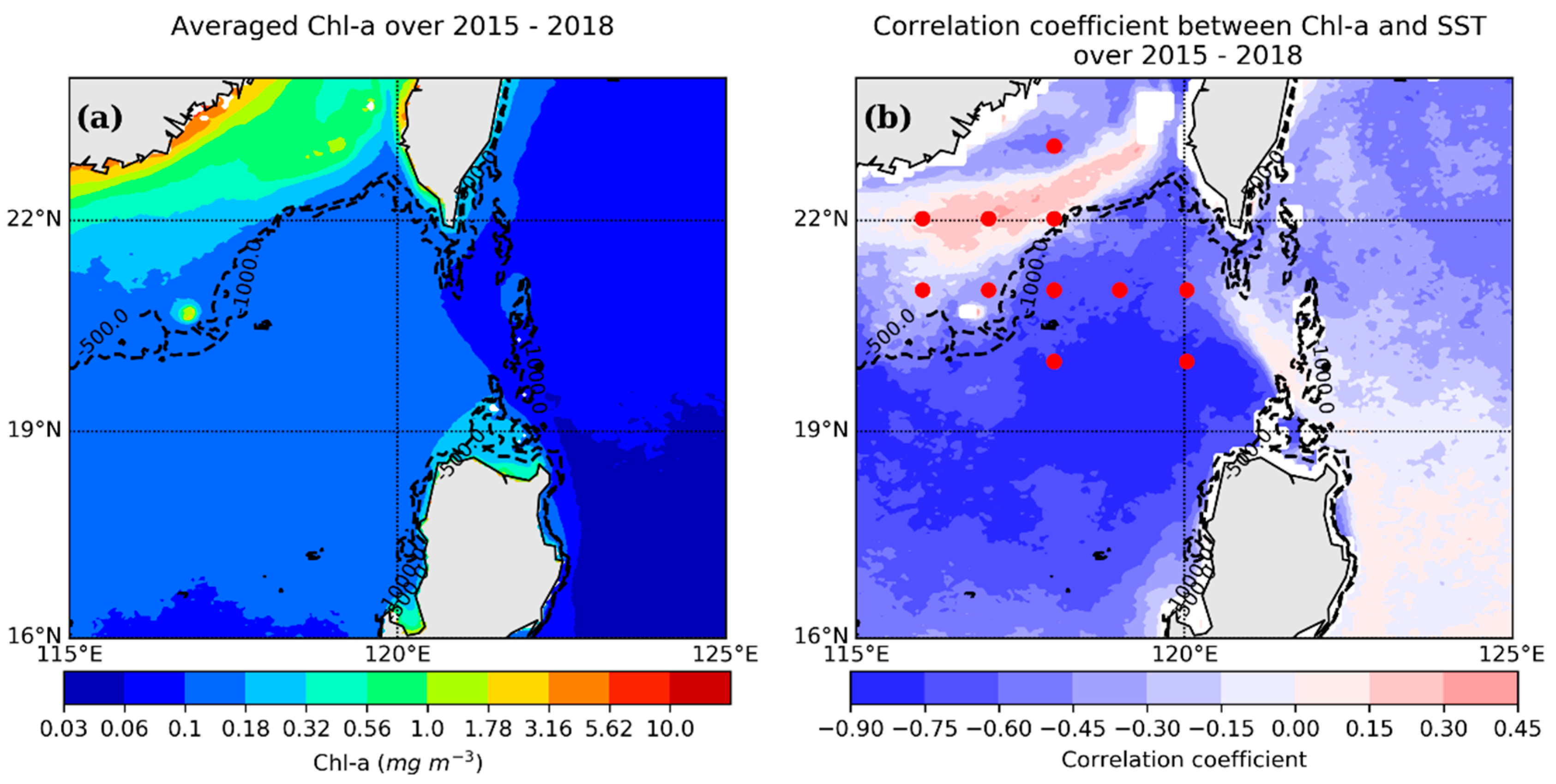
2.1. Study Area
2.2. Chl-a
2.3. SST
2.4. Cross-Validation Data
2.5. In Situ Dataset
3. Methods
3.1. DINEOF
3.2. DINCAE
- The input layer is used to receive the training datasets (training phase) and test datasets (reconstruction phase).
- Encoding layers are equivalent to the singular value decomposition (SVD) in DINEOF, which can effectively reduce the dimensionality of the input data in order to simplify the complexity of the required computing used in the neural networks. The work of the convolution layer is to extract the features of the input data, where the number and scale of these features depend on the depth of the convolution layer, which is also called the “convolution kernel size”. The work of the pooling layer is to compress the features extracted by the convolution layers, and the compression degree is determined by the type, size, and strides of the pooling layer. In this study, the size of convolution kernel was (3 × 3), and the maximum pooling was chosen, where pool size = (2,2) and strides = (2,2).
- Fully connected layers are equivalent to the hidden layer in the traditional feedforward neural network. Their function is to combine the extracted features nonlinearly. There were two full connection layers in this study, which were N/5 (rounded to the nearest integer) and N, where N is the number of neurons in the last pooling layer of the encoder.
- Decoding layers are composed of convolution layers and interpolation layers (nearest neighbor interpolation) to upsample the results. The interpolation layers are skip connected to the output of the pooling layers in order to capture small-scale structures that are lost in the encoding layers and fully connected layers [38].
- The output layer gives the results; that is, an array with a size of 240 × 192 × 2, including two parameters:
- : Chl-a scaled by the inverse of the expected error variance;
- : logarithm of the inverse of the expected error variance.
- (1)
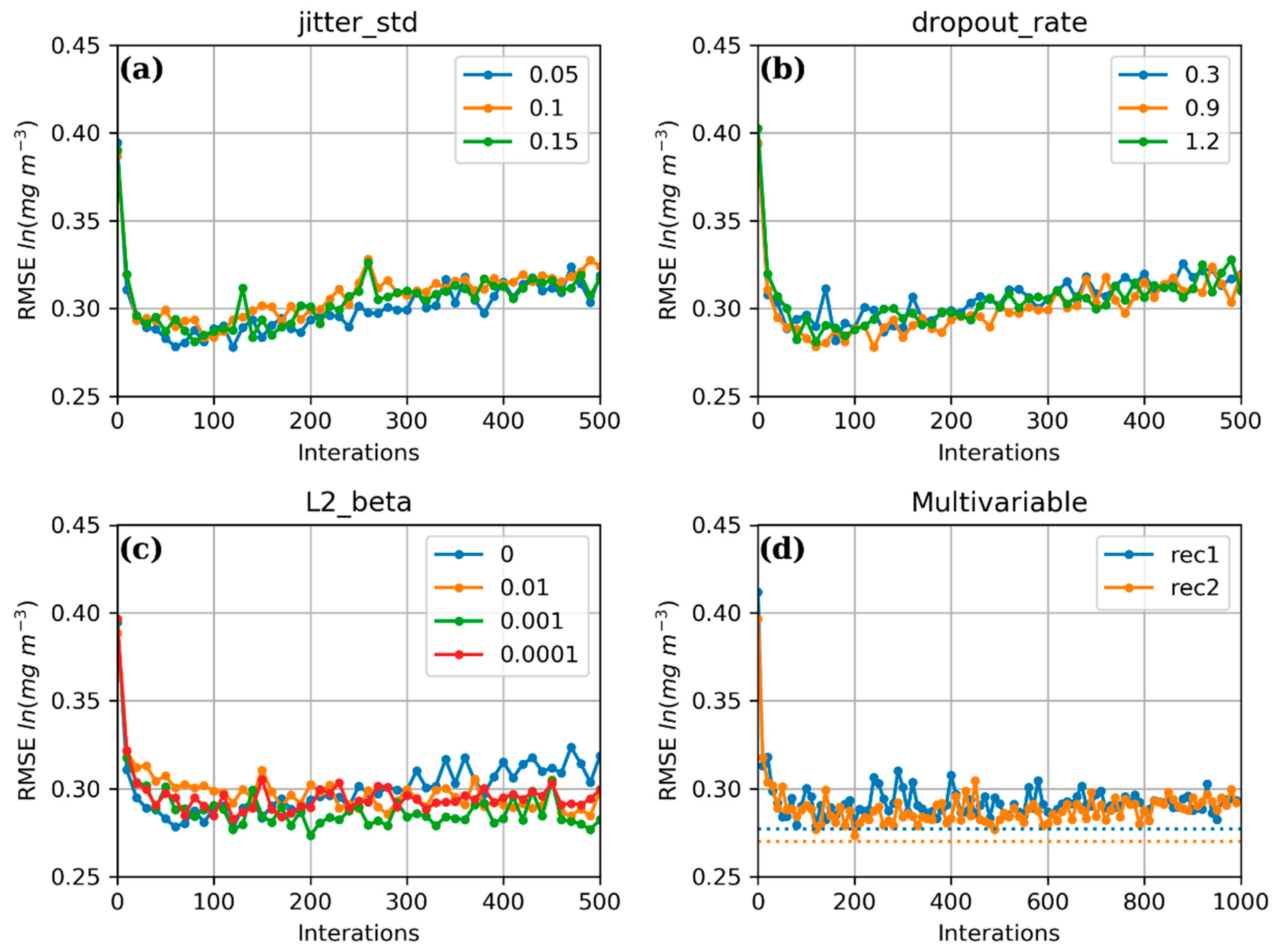
- A drop-out layer is introduced between the fully connected layers, and is randomly inactivated at a given rate (hereafter referred to as the dropout_rate, to be used later) of neurons in the fully connected layers.
- (2)
- Gaussian-distributed noise is added to the input data with a zero mean and a given standard deviation (hereafter referred to as jitter_std, to be used later).
- (3)
- A regularization technique is added to the Adam optimizer [39]. The basic idea of regularization is to add a penalty term to the loss function to punish the large weight and reduce the complexity of the model and prevent overfitting. In this study, the regularization parameter is set by , where L2 is the regularization term, is the weight for L2, and the value is given as L2_beta in the following discussion. Other standard parameters for the Adam optimizer are the learning rate = 0.001 and the exponential decay rates for the first moment estimates = 0.9 and the second moment estimates, = 0.999.
- (4)
- The activation function in the convolution layers uses Leaky-RELU [40] instead of the rectified linear unit (RELU) to prevent gradients from falling too fast:
4. Results
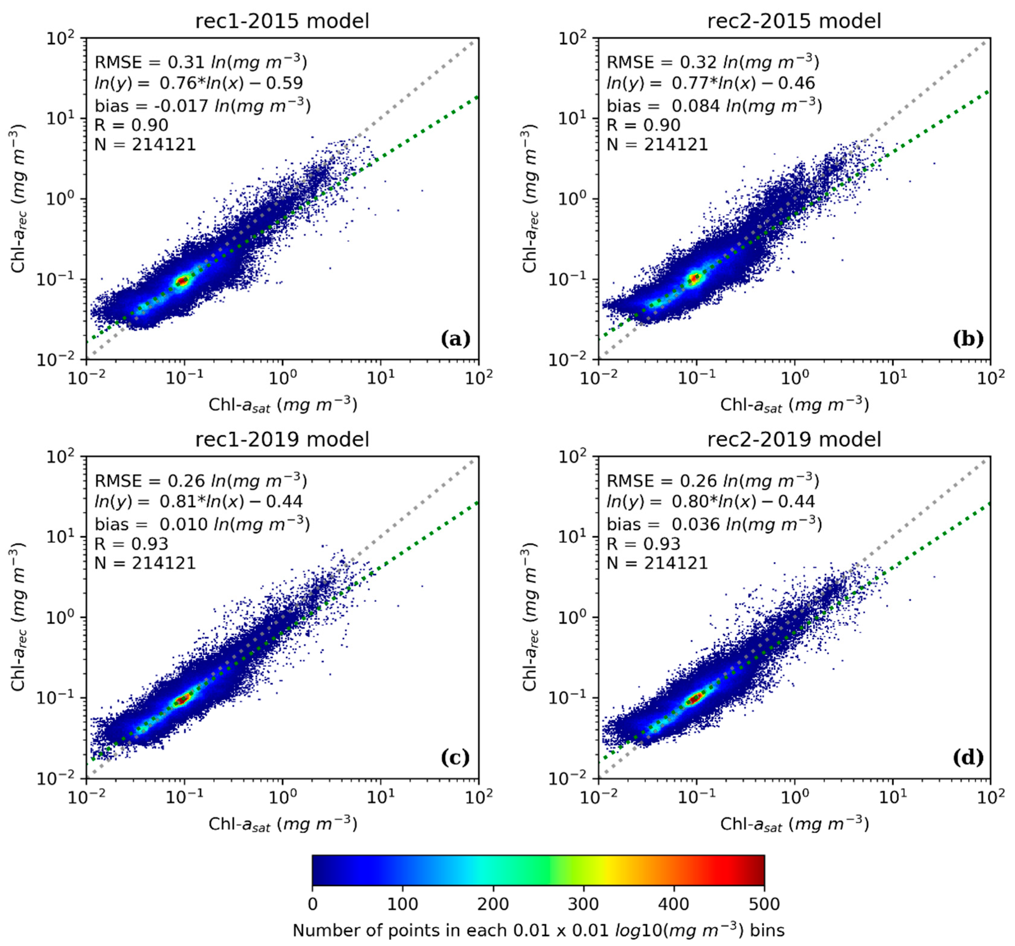
4.1. Reconstruction Statistics Using CV-Data
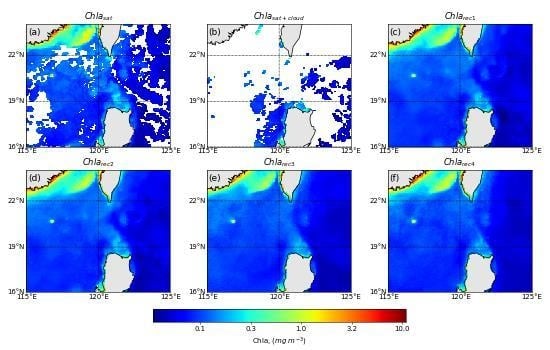
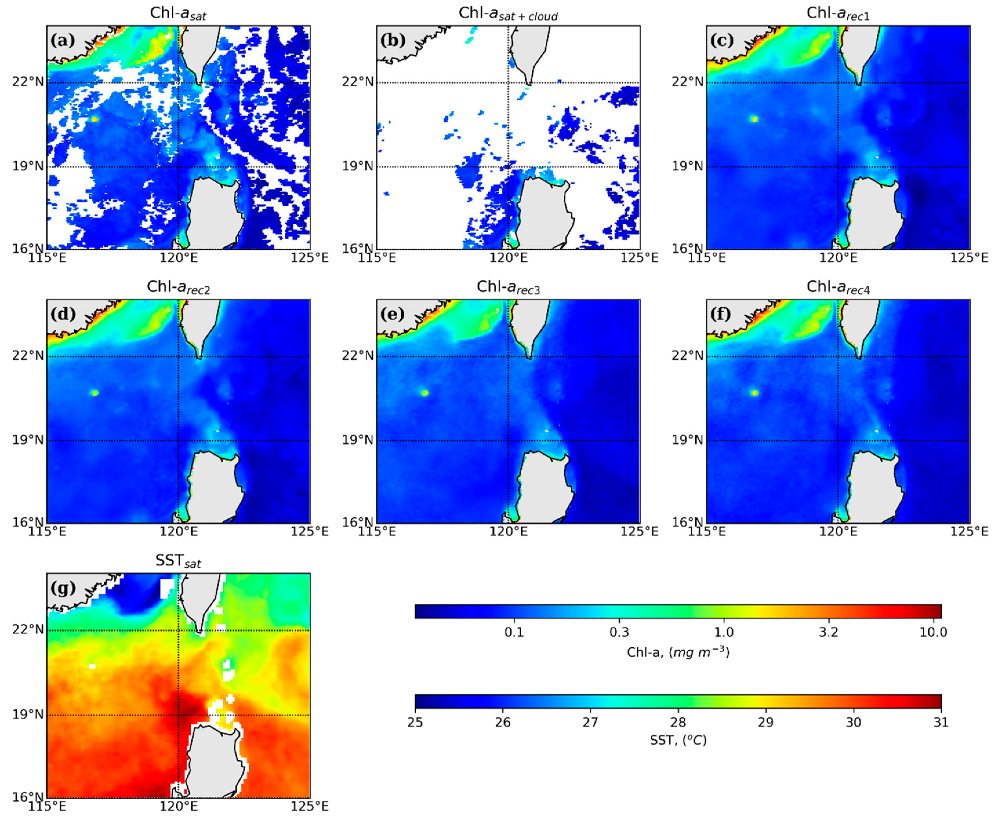
4.2. Spatial Distribution of Reconstruction for a Specified Day
4.3. Validation with In Situ Observations
5. Discussion
6. Conclusions
Author Contributions
Funding
Acknowledgments
Conflicts of Interest
References
- King, M.D.; Platnick, S.; Menzel, W.P.; Ackerman, S.A.; Hubanks, P.A. Spatial and temporal distribution of clouds observed by MODIS onboard the Terra and Aqua satellites. IEEE Trans. Geosci. Remote Sens. 2013, 51, 3826–3852. [Google Scholar] [CrossRef]
- Feng, L.; Hu, C. Cloud adjacency effects on top-of-atmosphere radiance and ocean color data products: A statistical assessment. Remote Sens. Environ. 2016, 174, 301–313. [Google Scholar] [CrossRef]
- Reynolds, R.W.; Smith, T.M.; Liu, C.; Chelton, D.B.; Casey, K.S.; Schlax, M.G. Daily High-Resolution-Blended Analyses for Sea Surface Temperature. J. Clim. 2007, 20, 5473–5496. [Google Scholar] [CrossRef]
- Group for High Resolution Sea Surface Temperature (GHRSST). Available online: https://www.ghrsst.org/ghrsst-data-services/products/ (accessed on 13 November 2019).
- Hosoda, K.; Sakaida, F. Global Daily High-Resolution Satellite-Based Foundation Sea Surface Temperature Dataset: Development and Validation against Two Definitions of Foundation SST. Remote Sens. 2016, 8, 962. [Google Scholar] [CrossRef] [Green Version]
- Bennett, A.F. Inverse Modeling of the Ocean and Atmosphere, 1st ed.; Cambridge University Press: Cambridge, UK, 2002. [Google Scholar]
- Saulquin, B.; Gohin, F.; Garrello, R. Regional Objective Analysis for Merging High-Resolution MERIS, MODIS/Aqua, and SeaWiFS Chlorophyll-a Data From 1998 to 2008 on the European Atlantic Shelf. IEEE Trans. Geosci. Remote Sens. 2011, 49, 143–154. [Google Scholar] [CrossRef] [Green Version]
- Beckers, J.M.; Rixen, M. EOF Calculations and Data Filling from Incomplete Oceanographic Datasets. J. Atmos. Ocean. Technol. 2003, 20, 1839–1856. [Google Scholar] [CrossRef]
- Alvera-Azcárate, A.; Barth, A.; Rixen, M.; Beckers, J.M. Reconstruction of incomplete oceanographic data sets using empirical orthogonal functions: Application to the Adriatic Sea surface temperature. Ocean Model. 2005, 9, 325–346. [Google Scholar] [CrossRef] [Green Version]
- Miles, T.N.; He, R.; Li, M. Characterizing the South Atlantic Bight seasonal variability and cold-water event in 2003 using a daily cloud-free SST and chlorophyll analysis. Geophys. Res. Lett. 2009, 36. [Google Scholar] [CrossRef] [Green Version]
- Abraham, E.R. The generation of plankton patchiness by turbulent stirring. Nature 1998, 391, 577–580. [Google Scholar] [CrossRef]
- Tang, D.; Kester, D.R.; Ni, I.H.; Kawamura, H.; Hong, H. Upwelling in the Taiwan Strait during the summer monsoon detected by satellite and shipboard measurements. Remote Sens. Environ. 2002, 83, 457–471. [Google Scholar] [CrossRef]
- Lin, J.; Cao, W.; Wang, G.; Hu, S. Satellite-observed variability of phytoplankton size classes associated with a cold eddy in the South China Sea. Mar. Pollut. Bull. 2014, 83, 190–197. [Google Scholar] [CrossRef] [PubMed]
- Shiozaki, T.; Chen, Y.-L.L. Different mechanisms controlling interannual phytoplankton variation in the South China Sea and the western North Pacific subtropical gyre: A satellite study. Adv. Space Res. 2013, 52, 668–676. [Google Scholar] [CrossRef]
- Volpe, G.; Nardelli, B.B.; Cipollini, P.; Santoleri, R.; Robinson, I.S. Seasonal to interannual phytoplankton response to physical processes in the Mediterranean Sea from satellite observations. Remote Sens. Environ. 2012, 117, 223–235. [Google Scholar] [CrossRef]
- Alvera-Azcárate, A.; Barth, A.; Beckers, J.M.; Weisberg, R.H. Multivariate reconstruction of missing data in sea surface temperature, chlorophyll, and wind satellite fields. J. Geophys. Res. Oceans 2007, 112. [Google Scholar] [CrossRef] [Green Version]
- Sirjacobs, D.; Alvera-Azcárate, A.; Barth, A.; Lacroix, G.; Park, Y.; Nechad, B.; Ruddick, K.; Beckers, J.-M. Cloud filling of ocean colour and sea surface temperature remote sensing products over the Southern North Sea by the Data Interpolating Empirical Orthogonal Functions methodology. J. Sea Res. 2011, 65, 114–130. [Google Scholar] [CrossRef]
- Yao, Z.; He, R. Cloud-free sea surface temperature and colour reconstruction for the Gulf of Mexico: 2003–2009. Remote Sens. Lett. 2012, 3, 697–706. [Google Scholar] [CrossRef]
- Li, Y.; He, R. Spatial and temporal variability of SST and ocean color in the Gulf of Maine based on cloud-free SST and chlorophyll reconstructions in 2003–2012. Remote Sens. Environ. 2014, 144, 98–108. [Google Scholar] [CrossRef]
- Guisan, A.; Zimmermann, N.E. Predictive habitat distribution models in ecology. Ecol. Model. 2000, 135, 147–186. [Google Scholar] [CrossRef]
- Elith, J.; Graham, C.H.; Anderson, R.P.; Dudík, M.; Ferrier, S.; Guisan, A.; Hijmans, R.J.; Huettmann, F.; Leathwick, J.R.; Lehmann, A. Novel methods improve prediction of species’ distributions from occurrence data. Ecography 2006, 29, 129–151. [Google Scholar] [CrossRef] [Green Version]
- Smoliński, S.; Radtke, K. Spatial prediction of demersal fish diversity in the Baltic Sea: Comparison of machine learning and regression-based techniques. ICES J. Mar. Sci. 2016, 74. [Google Scholar] [CrossRef] [Green Version]
- Barth, A.; Alvera-Azcárate, A.; Licer, M.; Beckers, J.M. DINCAE 1.0: A convolutional neural network with error estimates to reconstruct sea surface temperature satellite observations. Geosci. Model Dev. Discuss. 2019, 2019. [Google Scholar] [CrossRef]
- Chicco, D.; Sadowski, P.; Baldi, P. Deep autoencoder neural networks for gene ontology annotation predictions. In Proceedings of the 5th ACM Conference on Bioinformatics, Computational Biology, and Health Informatics (BCB ’14), Newport Beach, CA, USA, 20–23 September 2014; pp. 533–540. [Google Scholar]
- Jouini, M.; Lévy, M.; Crépon, M.; Thiria, S. Reconstruction of satellite chlorophyll images under heavy cloud coverage using a neural classification method. Remote Sens. Environ. 2013, 131, 232–246. [Google Scholar] [CrossRef]
- Chapman, C.; Charantonis, A.A. Reconstruction of subsurface velocities from satellite observations using iterative self-organizing maps. IEEE Geosci. Remote Sens. Lett. 2017, 14, 617–620. [Google Scholar] [CrossRef]
- Patil, K.; Deo, M.C. Prediction of daily sea surface temperature using efficient neural networks. Ocean Dyn. 2017, 67, 357–368. [Google Scholar] [CrossRef]
- Krasnopolsky, V.; Nadiga, S.; Mehra, A.; Bayler, E.; Behringer, D. Neural networks technique for filling gaps in satellite measurements: Application to ocean color observations. Comput. Intell. Neurosci. 2016, 2016, 6156513. [Google Scholar] [CrossRef] [PubMed] [Green Version]
- Jo, Y.; Kim, D.; Kim, H. Chlorophyll Concentration Derived from Microwave Remote Sensing Measurements USING Artificial Neural Network Algorithm. J. Mar. Sci 2018, 26, 102–110. [Google Scholar] [CrossRef]
- Chen, Y.L.L.; Chen, H.-Y.; Tuo, S.-H.; Ohki, K. Seasonal dynamics of new production from Trichodesmium N2 fixation and nitrate uptake in the upstream Kuroshio and South China Sea basin. Limnol. Oceanogr. 2008, 53, 1705–1721. [Google Scholar] [CrossRef] [Green Version]
- Liu, K.; Atkinson, L.; Quinones, R.; Talaue-McManus, L. Carbon and Nutrient Fluxes in Continental Margins: A Global Synthesis; Springer Science & Business Media: Berlin, Germany, 2010. [Google Scholar] [CrossRef]
- Liu, K.K.; Chao, S.Y.; Shaw, P.T.; Gong, G.C.; Chen, C.C.; Tang, T.Y. Monsoon-forced chlorophyll distribution and primary production in the South China Sea: Observations and a numerical study. Deep Sea Res. Part I Oceanogr. Res. Pap. 2002, 49, 1387–1412. [Google Scholar] [CrossRef]
- Liu, K.-K.; Tseng, C.-M.; Yeh, T.-Y.; Wang, L.-W. Elevated phytoplankton biomass in marginal seas in the low latitude ocean: A case study of the South China Sea. In Advances in Geosciences: Volume 18: Ocean Science (OS); World Scientific: Singapore, 2010; pp. 1–17. [Google Scholar] [CrossRef]
- McClain, C.R.; Signorini, S.R.; Christian, J.R. Subtropical gyre variability observed by ocean-color satellites. Deep Sea Res. Part II Top. Stud. Oceanogr. 2004, 51, 281–301. [Google Scholar] [CrossRef] [Green Version]
- Alvera-Azcárate, A.; Barth, A.; Sirjacobs, D.; Beckers, J.M. Enhancing temporal correlations in EOF expansions for the reconstruction of missing data using DINEOF. Ocean Sci. 2009, 5, 475–485. [Google Scholar] [CrossRef] [Green Version]
- Hilborn, A.; Costa, M. Applications of DINEOF to satellite-derived chlorophyll-a from a productive coastal region. Remote Sens. 2018, 10, 1449. [Google Scholar] [CrossRef] [Green Version]
- DINEOF—GHER. Available online: http://modb.oce.ulg.ac.be/mediawiki/index.php/DINEOF (accessed on 13 November 2019).
- Ronneberger, O.; Fischer, P.; Brox, T. U-Net: Convolutional Networks for Biomedical Image Segmentation. In Proceedings of the Medical Image Computing and Computer-Assisted Intervention—MICCAI 2015, Cham, Switzerland, 5–9 October 2015; pp. 234–241. [Google Scholar]
- Kingma, D.; Ba, J. Adam: A Method for Stochastic Optimization. arXiv 2014, arXiv:1412.6980. [Google Scholar]
- Maas, A.L.; Hannun, A.Y.; Ng, A.Y. Rectifier nonlinearities improve neural network acoustic models. In Proceedings of the 30th International Conference on Machine Learning, Atlanta, GA, USA, 16–21 June 2013. [Google Scholar]
- Abadi, M.; Agarwal, A.; Barham, P.; Brevdo, E.; Zheng, X. TensorFlow: Large-Scale Machine Learning on Heterogeneous Distributed Systems. arXiv 2015, arXiv:1603.04467. [Google Scholar]


| Reconstruction | Method | Input Satellite Data |
|---|---|---|
| rec1 | DINCAE | ln(Chl-a) |
| rec 2 | DINCAE | ln(Chl-a) and SST |
| rec 3 | DINEOF | ln(Chl-a) |
| rec 4 | DINEOF | ln(Chl-a) and SST |
| Index | Var Name |
|---|---|
| 1 | ln(Chl-a) anomalies scaled by the inverse of the error variance (zero if the data are missing) |
| 2 | Inverse of the error variance (zero if the data are missing) |
| 3–4 | Scaled ln(Chl-a) anomalies and inverse of error variance of the previous day |
| 5–6 | Scaled ln(Chl-a) anomalies and inverse of error variance of the following day |
| 7 | Longitude (scaled linearly between −1 and 1) |
| 8 | Latitude (scaled linearly between −1 and 1) |
| 9 | Cosine of the day of the year divided by 365.25 |
| 10 | Sine of the day of the year divided by 365.25 |
| 11 | SST anomalies scaled by the inverse of the error variance (zero if the data are missing) * |
| 12 | Scaled SST anomalies of the previous day * |
| 13 | Scaled SST anomalies of the following day * |
| Area | N, Mean, mg m−3 | Method | RMSE, ln(mg m−3) | Bias, ln(mg m−3) | R | Slope | Intercept |
|---|---|---|---|---|---|---|---|
| SCS | 145,476 0.34 | rec1 | 0.26 | −0.027 | 0.95 | 0.89 | −0.22 |
| rec2 | 0.25 | −0.019 | 0.96 | 0.90 | −0.19 | ||
| rec3 | 0.28 | −0.014 | 0.94 | 0.88 | −0.21 | ||
| rec4 | 0.32 | −0.005 | 0.92 | 0.92 | −0.12 | ||
| WPS | 140,985 0.11 | rec1 | 0.29 | 0.011 | 0.91 | 0.77 | −0.57 |
| rec2 | 0.28 | 0.025 | 0.91 | 0.78 | −0.53 | ||
| rec3 | 0.31 | 0.027 | 0.89 | 0.82 | −0.43 | ||
| rec4 | 0.33 | 0.009 | 0.88 | 0.81 | −0.47 |
| In Situ Data | Method | RMSE, ln(mg m−3) | Bias, ln(mg m−3) | R | Slope | Intercept |
|---|---|---|---|---|---|---|
| N = 20 mean = −1.61 ln(mg m−3) | rec1 | 0.38 | −0.14 | 0.925 | 0.81 | −0.16 |
| rec2 | 0.42 | −0.09 | 0.917 | 0.66 | −0.46 | |
| rec3 | 0.38 | −0.09 | 0.921 | 0.75 | −0.31 | |
| rec4 | 0.44 | −0.11 | 0.917 | 0.63 | −0.47 |
© 2020 by the authors. Licensee MDPI, Basel, Switzerland. This article is an open access article distributed under the terms and conditions of the Creative Commons Attribution (CC BY) license (http://creativecommons.org/licenses/by/4.0/).
Share and Cite
Han, Z.; He, Y.; Liu, G.; Perrie, W. Application of DINCAE to Reconstruct the Gaps in Chlorophyll-a Satellite Observations in the South China Sea and West Philippine Sea. Remote Sens. 2020, 12, 480. https://0-doi-org.brum.beds.ac.uk/10.3390/rs12030480
Han Z, He Y, Liu G, Perrie W. Application of DINCAE to Reconstruct the Gaps in Chlorophyll-a Satellite Observations in the South China Sea and West Philippine Sea. Remote Sensing. 2020; 12(3):480. https://0-doi-org.brum.beds.ac.uk/10.3390/rs12030480
Chicago/Turabian StyleHan, Zhaohui, Yijun He, Guoqiang Liu, and William Perrie. 2020. "Application of DINCAE to Reconstruct the Gaps in Chlorophyll-a Satellite Observations in the South China Sea and West Philippine Sea" Remote Sensing 12, no. 3: 480. https://0-doi-org.brum.beds.ac.uk/10.3390/rs12030480