Quantifying Long-Term Land Surface and Root Zone Soil Moisture over Tibetan Plateau


1
Department of European and Mediterranean Cultures, Architecture, Environment, Cultural Heritage, University of Basilicata, 75100 Matera, Italy
2
Faculty of Geo-Information Science and Earth Observation, University of Twente, Hengelosestraat 99, 7514 AE Enschede, The Netherlands
3
Department of Civil, Architectural and Environmental Engineering, University of Naples Federico II, Via Claudio 21, 80125 Napoli, Italy
4
Key Laboratory of Subsurface Hydrology and Ecological Effect in Arid Region of Ministry of Education, School of Water and Environment, Chang’an University, Xi’an 710054, China
*
Author to whom correspondence should be addressed.
Remote Sens. 2020, 12(3), 509; https://0-doi-org.brum.beds.ac.uk/10.3390/rs12030509
Submission received: 10 January 2020
/
Revised: 1 February 2020
/
Accepted: 3 February 2020
/
Published: 5 February 2020
(This article belongs to the Special Issue Microwave Remote Sensing for Hydrology)
Abstract
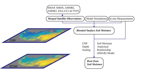
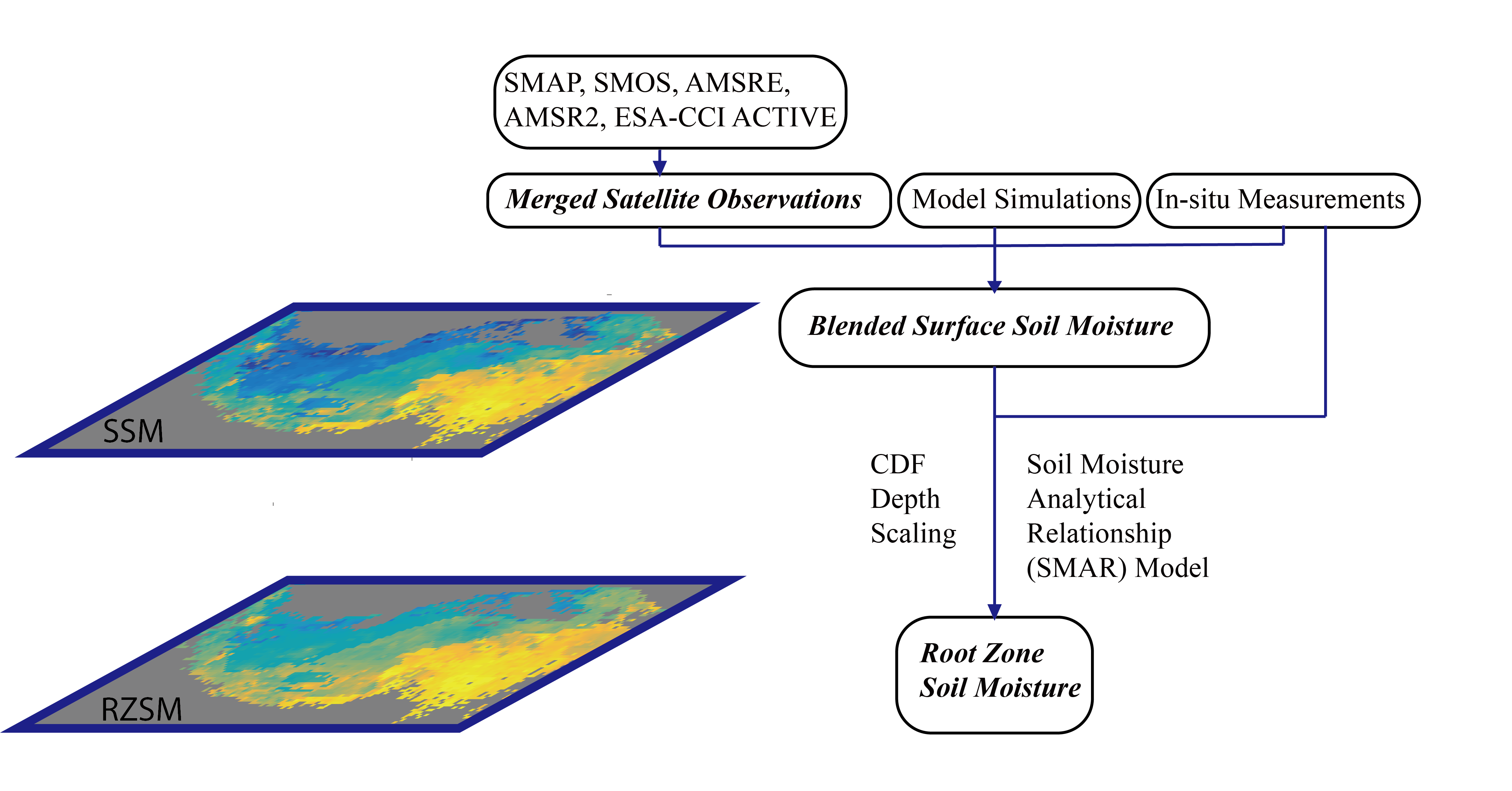
:It is crucial to monitor the dynamics of soil moisture over the Tibetan Plateau, while considering its important role in understanding the land-atmosphere interactions and their influences on climate systems (e.g., Eastern Asian Summer Monsoon). However, it is very challenging to have both the surface and root zone soil moisture (SSM and RZSM) over this area, especially the study of feedbacks between soil moisture and climate systems requires long-term (e.g., decadal) datasets. In this study, the SSM data from different sources (satellites, land data assimilation, and in-situ measurements) were blended while using triple collocation and least squares method with the constraint of in-situ data climatology. A depth scaling was performed based on the blended SSM product, using Cumulative Distribution Function (CDF) matching approach and simulation with Soil Moisture Analytical Relationship (SMAR) model, to estimate the RZSM. The final product is a set of long-term (~10 yr) consistent SSM and RZSM product. The inter-comparison with other existing SSM and RZSM products demonstrates the credibility of the data blending procedure used in this study and the reliability of the CDF matching method and SMAR model in deriving the RZSM.
1. Introduction
Soil moisture is a crucial land state variable that plays a critical role in energy partitioning and land-atmosphere interactions [1,2,3]. Comprehensions of soil moisture dynamics and trends can facilitate the identification of the interaction and feedbacks between the hydrological cycle and climate system [1,2,4,5]. In this context, the Tibetan Plateau represents as a natural laboratory, because it is an essential water tower in Asia and has significant effects on the Asian monsoon system, the atmospheric circulation, and the climate patterns [6]. Quantifying land surface soil moisture (SSM) and root zone soil moisture (RZSM) is indispensable for investigating the water and energy balance in the land-atmosphere system and the corresponding trends of climate change over the Tibetan Plateau. The observable climate change at the plateau scale can reshape the local environment and influence the hydrological cycles [7,8], but the systematic knowledge of the SSM and RZSM over the plateau are still limited [1,6,9].
There are three primary sources for the retrieval of soil moisture estimates, including in-situ measurements, satellite observations, and model simulations [10]. Several in-situ soil moisture observation networks, which include both SSM and RZSM, are routinely operated over Tibetan Plateau, namely the Third Pole Environment in situ component [11], the central Tibetan Plateau multi-scale soil moisture and temperature monitoring network [12], and the Tibetan Plateau Observatory of soil moisture and soil temperature (Tibet-Obs) [1]. The currently existing satellite observed SSM products include passive and active microwave observations. The Soil Moisture and Ocean Salinity (SMOS) [13] and the Soil Moisture Active Passive (SMAP) [14] are specialized to SSM monitoring, which are also producing the RZSM product based on SSM product. There are also several SSM products that are retrieved from satellites originally designed for other purposes, for example, the Advanced Microwave Scanning Radiometer (AMSR) SSM products retrieved while using the Land Parameter Retrieval Model [15], and the Advanced Scatterometer (ASCAT) SSM products retrieved with change detection method [16]. Besides, the reanalysis products (via integrating observations and land surface model simulations) can also provide soil both SSM and RZSM data, for example, the European Centre for Medium-Range Weather Forecasts Interim Reanalysis (ERA-Interim) [17,18] and the Global Land Data Assimilation System (GLDAS) [19].
Although satellites (in the past decades) have been developed and utilized as a nominal tool for monitoring SSM, the lifetime of a single satellite is limited. Furthermore, the data coverage period is not sufficient for climate change studies at the scale of Tibetan Plateau [20]. For this reason, several blended SSM datasets have been produced by scaling and blending satellite products with the model simulated SSM, such as the Climate Change Initiative SSM product (ESA-CCI) [21] and the Soil Moisture Operational Products System [22] from the U.S. National Oceanic and Atmospheric Administration [15]. It is to note that the SSM provides information on the degree of surface saturation that can be transformed into an estimate within the root-zone soil layer while using mathematical and statistical filters [23].
The RZSM is an important variable in the agricultural system, meteorological system, and hydrological cycle [24]. The saturation of RZSM affects the quantity of water that is absorbed by crop and it plays a significant role in the latent and sensible energy distribution and the precipitation redistribution [25]. The RZSM has a significant spatial variability and it has effects on the SSM through infiltration and capillary phenomenon in a non-linear way [26]. Nevertheless, most of the satellite observed/blended products have not included the RZSM, and only few RZSM product exists (e.g., the SMAP Level 4 product) [27]. It is challenging to quantify the RZSM over Tibetan Plateau due to the significant spatiotemporal variability and highly labor-time-consuming in-situ measurements. However, based on the non-linear relationship between SSM and RZSM [26], it is possible to estimate RZSM that is based on SSM data. The RZSM can be estimated from SSM by using filtering techniques [28] and analytical models [24,29]. Furthermore, Cumulative Distribution Function (CDF) matching could be used to derive RZSM with the depth scaling method [30].
It is to note that most of the existing SSM climatology scaling methods before data blending are performed based on the land surface model simulated SSM without the constraint of in-situ measurement [28,31,32,33]. It means that the results would be different when different land surface models were used, which may deviate from the in-situ observed SSM dynamics and physics [2]. This study will build upon in-situ measured SSM climatology to scale the model-simulated SSM, which will subsequently serve as the reference to scale satellite SSM products for further blending and, thus, generate a long-term (10yr) blended SSM dataset over Tibetan Plateau that is not yet available so far. The blended SSM will then be used to derive a decadal dataset of RZSM.
2. Materials and Methods
2.1. Datasets
There are three different types of SSM and RZSM datasets that are used in this research: in-situ measurements (Tibet-Obs), reanalysis products (ERA-Interim, GLDAS), and satellite observations (include AMSRE, AMSR2, SMOS, SMAP, and ESA-CCI products). Each dataset is available over different time spans, as displayed in Table 1.
2.1.1. In-Situ Datasets
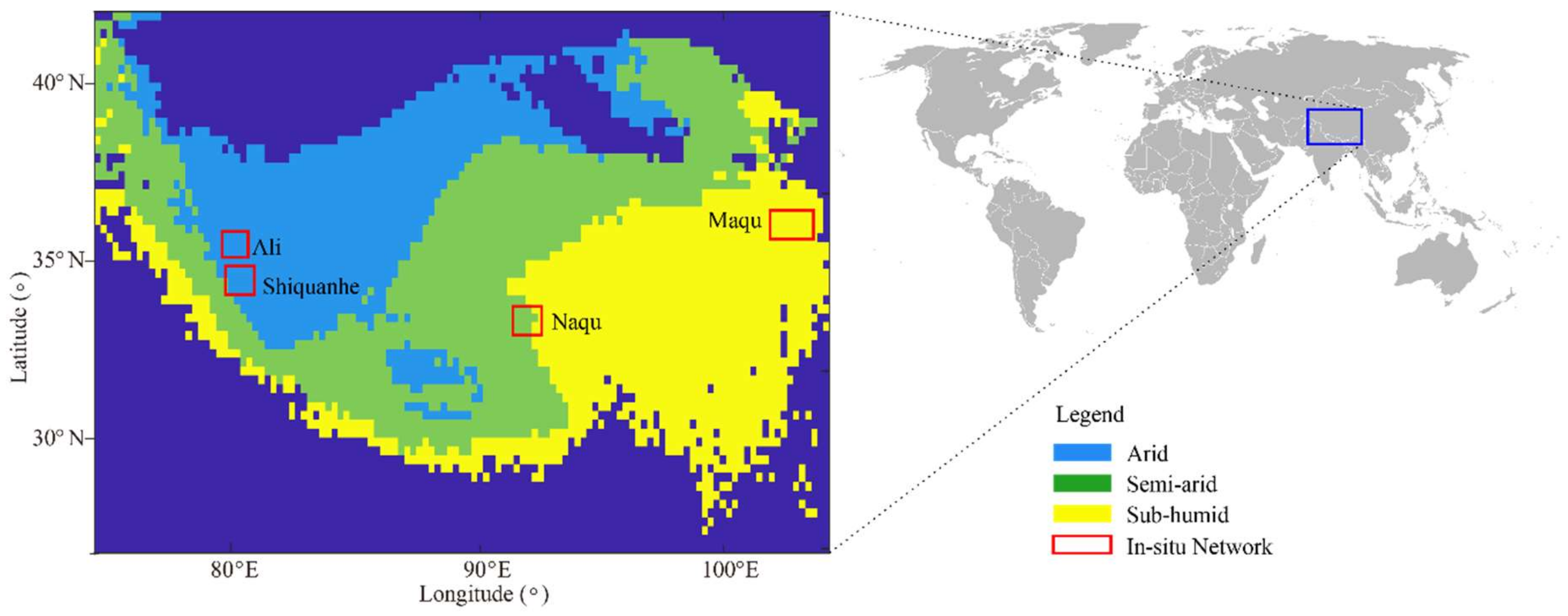
The Tibetan Plateau Observatory (Tibet-Obs) [1] includes SSM and RZSM measurements in Naqu semi-arid network (five stations), Maqu sub-humid network (twenty stations), and Ali-Shiquanhe arid network (twenty stations), which are using ECH2O probes to measure the dielectric permittivity and obtain volumetric soil moisture content with calibration equations. The averaged SSM and RZSM data of each network were used to produce the in-situ data reference product while using the climate zone classification based on FAO aridity index map. As a result, the averaged in-situ measured SSM and RZSM values of Naqu network are used to indicate SSM and RZSM in the semi-arid regions in FAO Aridity Index map, and Maqu network corresponds to the sub-humid area, and Ali and Shiquanhe both correspond to the arid area [2]. Figure 1 presents the location of Tibetan Plateau and the distribution of Tibet-Obs networks.
2.1.2. Satellite Datasets
All of the satellite data and reanalysis data in this research were resampled to a resolution of 0.25°, which is often adopted by land surface models. This is a trade-off between the higher resolution scatterometer data and the generally coarse passive microwave observations. The nearest-neighbor interpolation was used in the resampling step [34].
The VUA-NASA SSM product (AMSR-E) was derived from the Advanced Microwave Scanning Radiometer-Earth Observing System [15,35] while using the Land Parameter Retrieval Model. The SSM was derived from a forward radiative transfer model using a nonlinear iterative optimisation method and the microwave polarisation difference index of the brightness temperature. The SSM products that were used in this research were derived from C-band, as it has less signal attenuation from atmosphere and vegetation and less radio-frequency interference than the X-band [36,37].
The AMSR-2 SSM product is derived from the Advanced Microwave Scanning Radiometer 2 loaded on the Water GCOM-W1 satellite that was launched by the Japan Aerospace Exploration Agency [38]. The AMSR-2 is a follow-up of AMSR-E, since 3 July 2012 to provide a long-term satellite observation [39]. The data retrieval algorithm is similar to AMSR-E. Only the descending mode (01:30 a.m. local time) AMSR-E and AMSR-2 products were used while considering the limited uncertainties that were caused by temperature variations during night-time.
The SMOS product that was used in this research was the Level 3 descending SSM product derived by France National Centre for Space Studies (CNES). As one of the Earth Explorer Opportunity Missions from the European Space Agency (ESA), the SMOS satellite was launched with a 1.4 GHz L-Band radiometer on 2-November-2009 [40]. The L-band microwave emission is obtained from a zero-order radiative transfer equation while using the L-MEB biosphere model [41]. The multiangular observation helped SMOS to simultaneously obtain the SSM and ancillary information [41,42].
The SMAP product used in this research is the SMAP L3 Radiometer Global Daily data of descending orbit retrieved from L-band (1.41 GHz) brightness temperature of the passive microwave radiometer via the National Snow and Ice Data Center. NASA launched the SMAP satellite on 31-January-2015, and the observation target is a volumetric accuracy of 0.04 m3·m−3 in the top layer of the land surface every two to three days. The tau-omega model was operated after the open water area was corrected [43].
The ESA Climate Change Initiative (ESA-CCI) [44,45,46] ACTIVE products are merged by two of the SSM products that were retrieved from the Advanced Scatterometer (ASCAT), which loaded on the Meteorological Operational (METOP-A and METOP-B) satellites [16], using the change detection method [16,23]. The original SSM products are provided as saturation degrees (0%–100%), and they were used to multiply porosity values that were provided by ESA-CCI [47] over the Tibetan Plateau to yield the volumetric soil moisture content.
2.1.3. Reanalysis Dataset
ERA-Interim SSM and RZSM product (ERA-Interim) is a part of the Land Data Assimilation System that was produced by the European Centre for Medium-Range Weather Forecasts [17]. The volumetric soil moisture content was produced at four layers, and the daily average soil moisture of the first layer (0–7 cm) is the one to be used in this research as a reference SSM dataset in climatology scaling before data blending [33]. Additionally, the daily average value of the root zone layer is used for comparison with the RZSM products generated in this research.
NASA and the National Oceanic and Atmospheric Administration (NOAA) developed the Global Land Data Assimilation System (GLDAS) [19]. It applies the land surface models with meteorological observations as the forcing. The data assimilation approaches are used to adjust the model states. The GLDAS daily SSM and RZSM data were compared with the SSM and RZSM products in this research.
2.2. Methodology
2.2.1. Methods Description
(a) Cumulative Distribution Function (CDF) Matching
The CDF matching approach has been widely used for removing the systematic differences between two series, such as bias reduction in satellite-observed SSM [31,32,33,48]. The method can also be used to transfer the data of different areas [25] and upscale the point data measurements [26]. To implement CDF matching, the first step is ranking the reference, and the to-be scaled data. Second, calculate the differences between the corresponding data of two ranked datasets and then perform linear regression analysis segment by segment on the CDF curves of the calculated differences and the to-be scaled data. Lastly, use the CDF matching parameters to scale the to-be scaled data for each segment [49]. The scaled data would show a similar pattern with the CDF curve of the reference data, which indicates that the systematic difference between the original observation and the reference data has been eliminated. It is worth noting that, among four conventional scaling methods (linear regression, linear rescaling, MIN/MAX correction, and CDF matching), the CDF matching shows the best performance [48], and it only requires one year data to calibrate [33].
(b) Least Squares Method
The objective of least squares method is determining optimal weights for merging two or three independent datasets while using a weighted average method. It is one of the most widely used data assimilation methods, which has been used in numerous studies since it was shaped into the current form. It was used to blend remotely sensed and model-simulated SSM products with or without in-situ data constraint [50].
When the target product is merged as a linear combination of single products, the equation of data merging can be expressed as:
where , , are the relative weights of data sets a, b, c, and is the target merged product. The merged product is unbiased optimal if the summation of optimal weights is one. It is a constraint of the solution to the estimation error variance minimization problem. Accordingly, the solution to minimize the error variance of relate to weights , , could be calculated from relative error variance , , . The to be minimised error variance of can be expressed as
Assume and , the equations to determine the relative weights by using relative errors are presented below:
The method can also work in two datasets situation. The equations are presented below:
(c) Triple Collocation Analysis
Triple collocation was used to determine the relative errors of each input datasets in this research. Triple collocation is an error estimation method that can be used to estimate the random error variances and systematic biases in different datasets without reliable reference data sets. It improved the accuracy of calibration or validation when compared with the dual comparisons that were widely used before. To implement the triple collocation method, three independent datasets should be used jointly to determine the relative errors [51]. The error variances of each dataset can be presented as:
where , , are the data variances and , , are the errors variances. , , are data covariance.
(d) Soil Moisture Analytical Relationship (SMAR) Model
The SMAR model is a physically based infiltration model with two layers, which aims to estimate the RZSM (the second soil layer) from the SSM (the first soil layer) time series.
where [-] is the relative saturation of the second soil layer, [-] is the wilting point of the second soil layer, and [-] represents the fraction of soil water infiltrating from the top layer to the lower layer. Coefficients a and b represent:
where [] is the soil water loss (evapotranspiration and percolation) coefficient, [-] represents the porosity of layer of soil, and [L] is the soil depth of layer.
As it is an analytical method, the parameters of the SMAR model were mathematically derived under some assumptions. First, when compared with infiltration, capillary rise and lateral flow are negligible in water mass exchange between two layers. Second, the water exchange happens immediately and ends within one day when soil water in the first layer exceeds field capacity, with an infinite permeability. Third, the soil water loss of the second layer decreases linearly from a relatively humid (does not include the real humid condition with a significant non-linear water loss function) condition to the wilting point [24,29,52].
2.2.2. Processing Procedures
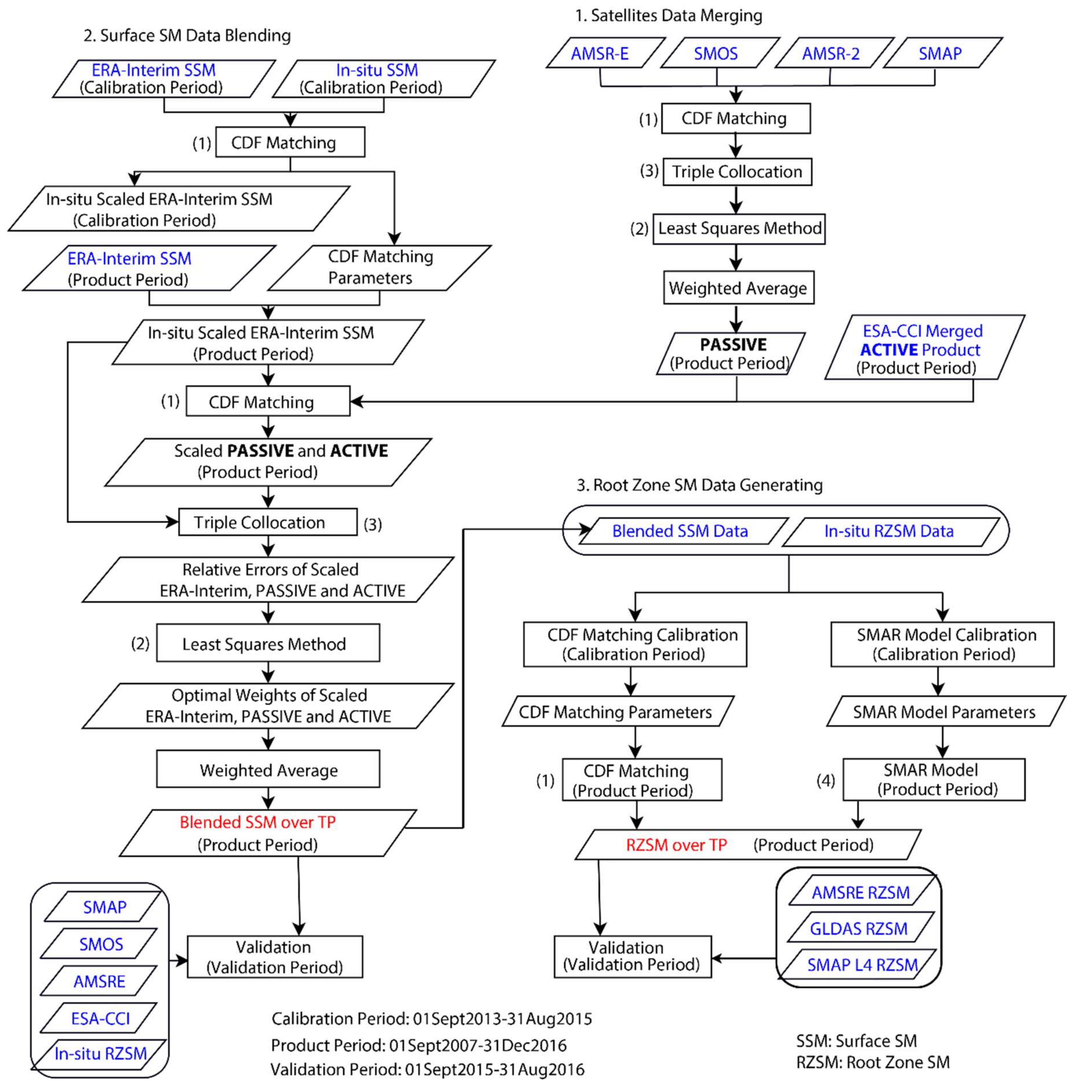
The central processing procedures include satellite data merging, SSM data blending, and RZSM generating (the flowchart of processing procedure is presented in Figure 2). The division of the calibration period, the product period, and the validation period were based on data availability.
(a) Satellite Data Merging
Satellite data merging aims to merge all of the available passive microwave observation data into one PASSIVE product. The ESA-CCI PASSIVE product [44,45,46] was merged in the same way using TRMM Microwave Imager, WindSat Radiometer, AMSRE, AMSR2, and SMOS, but without SMAP, so, it will be used for comparison. As for active microwave observations, the ESA-CCI Merged ACTIVE products were used directly, as it was merged using Advanced Scatterometer (Metop) which will be applied the same way for this research. Nevertheless, the approach in our research differs from ESA-CCI, in that the in-situ SSM climatology is taken into account before the final SSM blending.
● Rescaling while using CDF matching
Differences in sensor specifications, particularly in microwave frequency and spatial resolution, result in different absolute SSM values from AMSR2, SMOS, SMAP, and AMSR-E. It is needed to scale datasets into a common climatology using the CDF matching method. The climatology of AMSR-E was selected as the reference, because the AMSR-E SSM retrievals were identified as more accurate than other passive products due to the relatively low microwave frequency and high spatio-temporal resolution of the sensor [33].
● Error Characterization using triple collocation
Error characterization aims to obtain the relative errors (stationary average random errors) of each dataset while using triple collocation analysis. The triple collocation analysis was performed for those pixels, where two or three datasets overlapped and were uncorrelated [53]. Furthermore, the uncertainties of the target product (PASSIVE product) can also be determined from the error variances of every single product.
● Optimal weights calculated while using the least-squares method and weighted averaging
The scaled satellites data were merged using a weighted average on a pixel basis which considers the error properties of each dataset. The optimal weights for the weighted average were determined by the relative error variances of all of the input datasets over each specific merging period using the least-squares method. The merging method works in both three datasets and two datasets cases, as relative errors of each dataset have been determined. However, for specific locations, triple collocation analysis does not yield valid error estimates. In such cases, the weights were equally distributed amongst the available datasets.
(b) SSM Data Blending
● Rescaling while using CDF matching method
First, as a reference dataset, ERA-Interim SSM products over the Calibration Period was scaled based on the obtained in-situ data climatology using CDF matching, which can also produce the seasonal CDF matching parameters for climatology scaling of ERA-Interim data over the Product Period (see Figure 2). The above-mentioned seasons are defined as Monsoon (May–October), Transaction1 (April), Winter (December-March), and Transction2 (November). Subsequently, the ERA-Interim SSM data over Product Period were scaled using the seasonal CDF matching parameters.
Next, another CDF matching was performed to scale each merged satellite dataset (PASSIVE and ACTIVE products generated in satellite data merging step) based on the in-situ scaled ERA-Interim data climatology over the Product Period.
- Error Characterization using triple collocation
- The relative errors among the scaled PASSIVE, ACTIVE, and ERA-Interim products were calculated while using the triple collocation method, which used three collocated datasets to constrain the relative error variance determination without a manually decided reference.
- Optimal weight calculation using the least-squares method and weighted averaging
- Similar with satellite data merging, a weighted average was used to merge scaled PASSIVE, ACTIVE, and ERA-Interim products over the Product Period and the optimal weights were obtained based on the relative errors while using least squares method.
(c) Deriving RZSM
● Depth Scaling Using CDF Matching
CDF matching method was used to calculate RZSM from the blended SSM data. The Tibet-Obs in-situ measured SSM and RZSM datasets [1] over the Calibration Period were used to generate the depth scaling parameters. Note that the RZSM refers to a mean value of the SM in the 0–80 cm depth:
where is the index of the soil layer; [L3L−3] is the RZSM; [L] is the soil layer depth; and, [L3L−3] is soil moisture in the soil layer. The specific Tibet-Obs product used in this research includes the soil moisture data at the depth of 5 cm, 10 cm, 20 cm, 40 cm, and 80 cm.
The scaling parameters of the fifth-order polynomial fitting function were generated from the SSM and the differences between the corresponding values of ranked SSM and RZSM. Gao et al. [30] identified the fifth-order polynomial as the optimal choice based on a pre-analysis to define the fitting function for depth scaling. The scaling parameters were used to estimate the predicted difference between SSM and RZSM over the Product Period; then, the predicted RZSM were generated while using blended SSM and the predicted differences.
● RZSM Estimation Using SMAR model
In the four in-situ measurement networks of Tibet-Obs (Ali, Shiquanhe in an arid region, Naqu in semi-arid region, and Maqu in sub-humid region), SMAR model parameters were derived mathematically over the one-year Calibration Period while using the SSM and RZSM (same with the datasets used for depth scaling using CDF Matching). The parameters were applied over the entire Product Period.
3. Results
3.1. SSM Product
3.1.1. Merged Satellites SSM Product
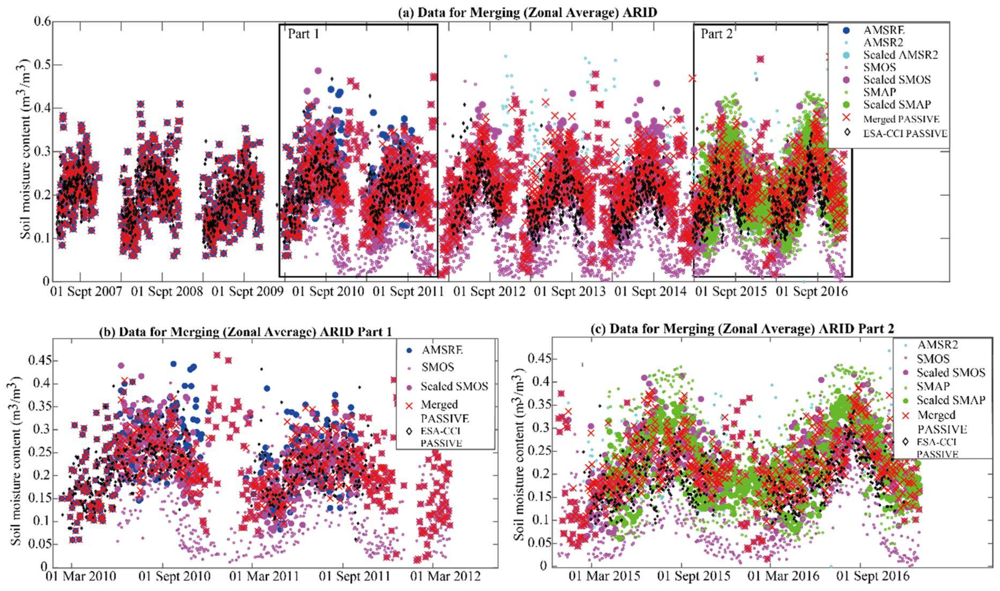
The rescaling procedure kept the seasonal dynamics and adjusted the absolute values of original datasets (e.g., SMOS, AMSR2, and SMAP SM products), follows the procedures by Liu et al. [33]. The consistency is a necessary condition for the following merging procedures. Figure 3 highlights such consistency of the time sires, where all the time series of raw data, scaled data, and merged data are presented. The merged PASSIVE data are close to the ESA-CCI PASSIVE product, but with a wider fluctuation.
The raw satellites data were scaled and merged over each merging period, as presented in Table 1. For the merging periods of S1 and S3, as only one satellite dataset available, the merged SSM uses only that dataset. For S2, the merging time is relatively short, and the data of SMOS is much less than AMSRE, but these conditions did not influence the performance of triple collocation. For S4, the relative errors of SMOS and AMSR2 are similar, so the optimal weights for merging the two are similar. Table 2 presents the specific averaged relative errors and Optimal Weights over each merging period (for the explanation of parameters see Section 2.2). In general, AMSR data were assigned higher weights than SMOS data.
In the merging period S1 and S3, only one satellite dataset included in the merged product, which means that the weight is 1 for that satellite dataset. Otherwise, the merging weights were calculated from relative errors; the pixels without valid relative errors were set as the equal weights. As AMSRE and AMSR2 have low errors, the weights of them are relatively high. SMOS and SMAP have similar relative errors and they are higher than those of AMSRE and AMSR2, as such, their weights are relatively low. However, the difference is small, especially in the period of S5.
3.1.2. Blended SSM Product
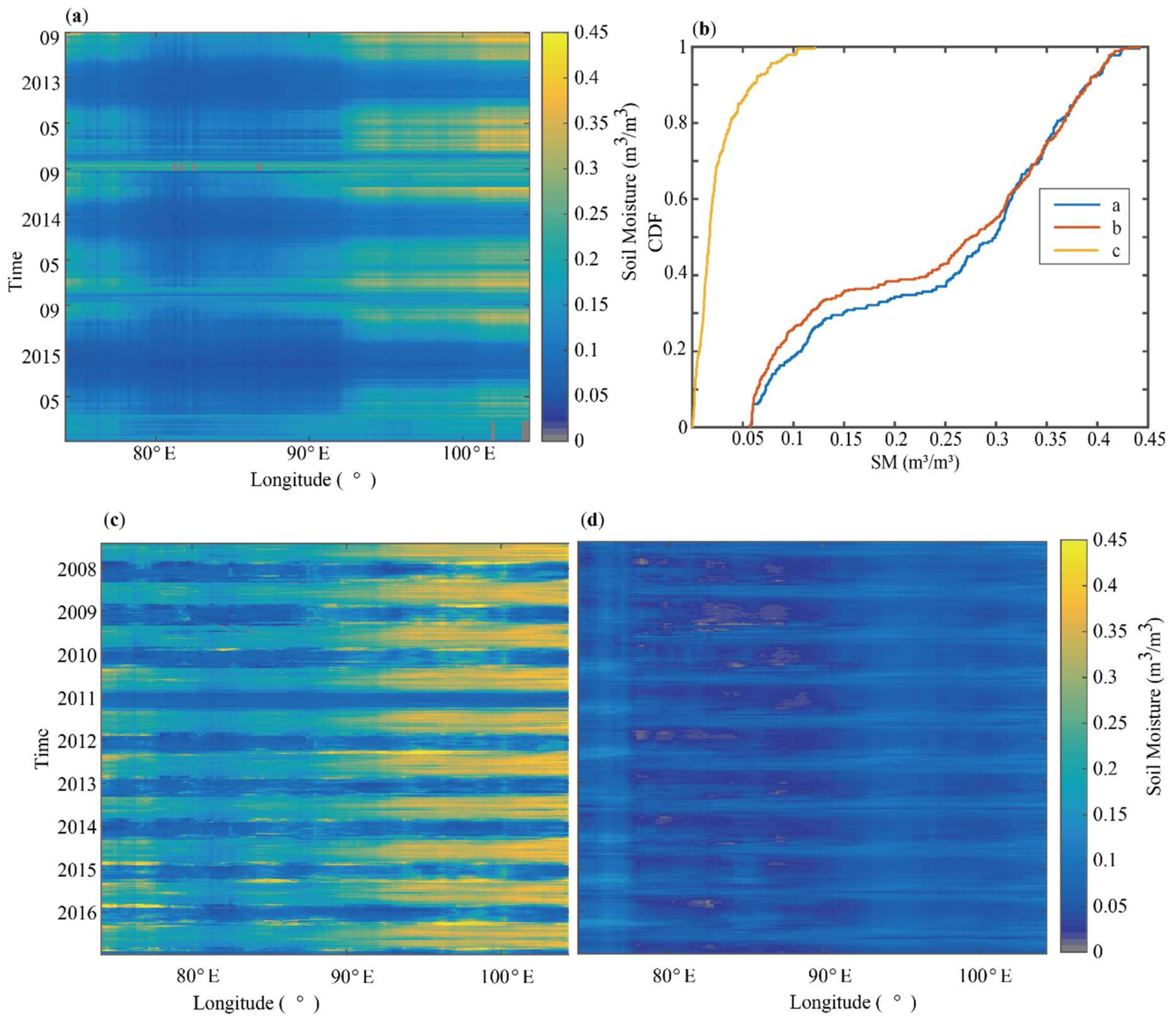
First, the ERA-Interim SSM data were scaled based on the in-situ climatology. Figure 4 presents the time-longitude diagrams of in-situ data, the original ERA-Interim, and the scaled ERA-Interim, as well as an example illustrating how the CDF matching works (Figure 4c). Figure 4a shows the in-situ data climatology over the Calibration Period. The sub-humid regions (eastern part of the time-longitude diagram) show a significant seasonal difference, while the SM data in the western part show relatively low values in both the monsoon season and the winter. The original ERA-Interim SM data did not show apparent seasonal change as compared with the in-situ climatology in Figure 4a, as presented in Figure 4d. After scaling, the scaled ERA-Interim product shows a similar pattern with the time-longitude diagram of in situ climatology (Figure 4d). The volumetric water content is around 0.35 (m3/m3) in the monsoon season, while it is around 0.07 (m3/m3) in the winter.
Subsequently, the scaled ERA-Interim SM product was used to scale the PASSIVE and ACTIVE products. Although the original PASSIVE and ACTIVE products show some seasonal and spatial dynamics, they show different dynamic ranges and absolute values. Moreover, the PASSIVE product overestimated the SSM over Tibetan Plateau, especially during the monsoon seasons. While the ACTIVE one underestimates SSM over the winter. After scaling, scaled PASSIVE and ACTIVE data both show a similar climatology with the scaled ERA-Interim data, as well as the dynamic range of SSM. The effect of climatology scaling was significant, and the averaged SSM in the sub-humid region of Tibetan Plateau was up to 0.40 (m3/m3) before scaling. After scaling, the absolute values of PASSIVE products changed based on the systematic difference with the reference data (scaled ERA-Interim).
The blending of these scaled SSM products was implemented in two situations: first, blending the three collocated SSM data, where the datasets have enough triplets; second, blending the rest of data, where one satellite data individually collocates with the scaled ERA-Interim data, but not collocate with another satellite data (i.e., no triplets). To tackle the first situation, the data number of each product and the corresponding triplets’ number was checked. The ERA-interim product has more than 3500 data across the southern and eastern part of Tibetan Plateau and have many data in the arid zones. PASSIVE and ACTIVE products have less data number. The eastern regions have around 1200 triplets, while some of the western regions have less than 400 triplets. Only the data with more than 100 observation triplets were presented, as 100 observation triplets are required for a reliable estimation of the relative errors among the three SSM products [54]. Next, the minimum correlation coefficient among the three collocated SSM products was calculated to check whether the identified number of triplets is statistically significant to apply with triple collocation method. The distribution of minimum correlation coefficient is relatively equal when compared with the triplets’ number and most of the areas are with a minimum correlation coefficient of more than 0.15, which is required for a sample with more than 100 data to achieve the statistical significance. The area with triplet number > 100 (where the P-value < 0.05) are all statistically significant to be applied with triple collocation method to identify the relative errors.
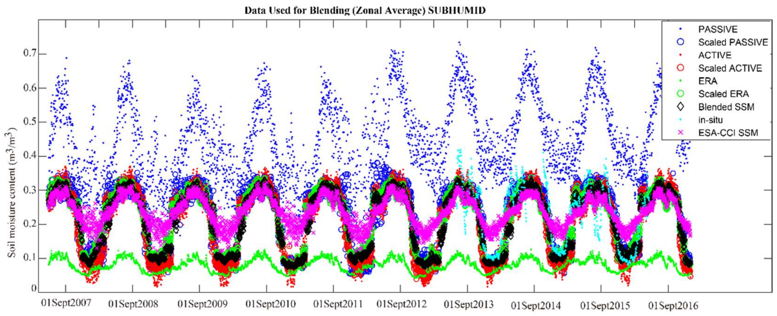
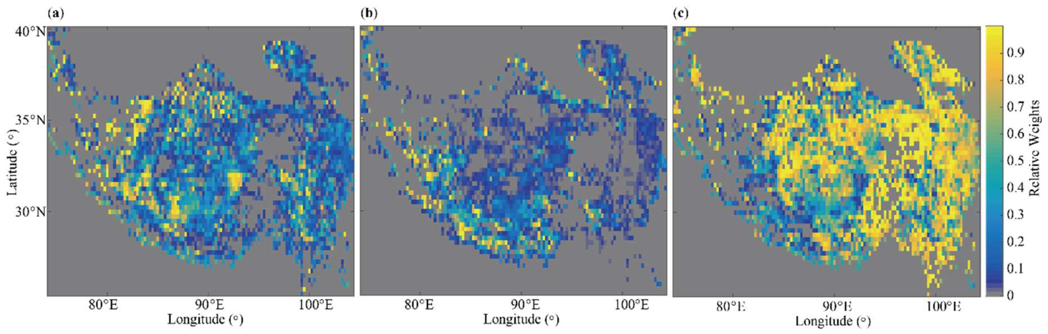
Figure 5 presents the time series of data that are involved in the data blending procedure. It is evident that scaled ERA-Interim, PASSIVE, ACTIVE data became align with each other, and the blended SSM, which constrained by the in-situ climatology, captured better the in-situ SSM dynamics when compared with ESA-CCI SSM product. Figure 6 shows the optimal weights of scaled ERA-Interim (a), PASSIVE (b), and ACTIVE (c) products, which were determined by the relative errors while using the least-squares method. Among the three SSM products, the ACTIVE product has the smallest average relative error (0.0032 cm3cm−3), while the highest weight (0.60) contributing to the blended products. The average weight of the PASSIVE product is 0.14 and the scaled ERA-Interim product is 0.30. The reason why the merging weights of PASSIVE product are relatively low is the low SSM retrieval rate of passive satellites over the central and western Tibetan Plateau, which are arid or semi-arid regions [16].
The other situation is to blend the scaled satellite SSM data individually collocating with the scaled ERA-Interim data, but not collocating with each other. The weights for blending were determined from the scaled PASSIVE product and ERA-Interim, or the scaled ACTIVE product and ERA-Interim. For example, there were scaled PASSIVE data individually collocated with the scaled ERA-Interim, the average weight of scaled ERA-Interim is 0.4598, and the average weight of the scaled PASSIVE is 0.5403, corresponding with a relative error of 0.0123 cm3cm−3 and 0.0063 cm3cm−3, respectively.
3.2. RZSM Product
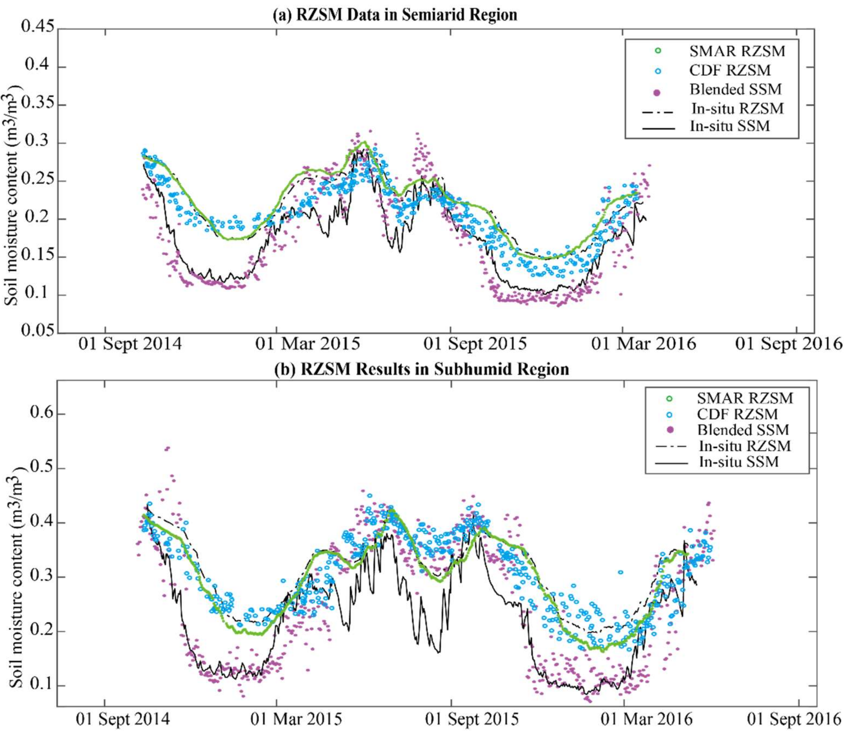
CDF matching is the first method that is used to generate RZSM. The calibration aims to generate CDF parameters of the scaling function for every single cell, which is a fifth-order polynomial aims to illustrate the non-linear relationship between the surface-root zone difference and the SSM data. Figure 7a presents the surface and root zone relationships found in the semiarid region. The RZSM is higher than SSM in the winter and lower in the monsoon season. The seasonal differences are low in semi-arid areas and are relatively evident in sub-humid regions. The RZSM in semi-arid region (Figure 7a) shows a smooth pattern with absolute values that are slightly higher than SSM in the winter and lower in the monsoon season. The results present that the RZSM estimation qualitatively kept the in-situ data climatology. The time series in Figure 7b is the averaged SSM and RZSM data in the sub-humid region. The way to generate the averaged in-situ RZSM was averaging soil moisture layer by layer across all stations due to the high heterogeneity of SSM and RZSM across Tibet-Obs stations.
Using the SMAR model is the second method to generate RZSM. The calibration of the model was based on the blended SSM data and in-situ RZSM over two years in three climate zones. The calibration of the SMAR model needs a continuous input time series, which requires some procedures to fill or skip the gaps. In this research, the gaps less than three days are interpolated, and the long gaps are skipped, and the time series were cut into several sections, and the calibration was carried out over the relatively long time series. Table 3 presents the calibrated parameters and root mean square errors. In semi-arid region, the calibration parameters are the most trustworthy as the root mean square error is the lowest. Figure 7 compares the RZSM results from both CDF method and SMAR model. In Semiarid region, the results are similar, while the SMAR model generated a smooth result and the CDF method result is highly dependent on the input data (blended SSM). In sub-humid region, the SMAR result is very close to the reference in-situ data after a short model warming up period. The results for arid region are not shown, due to too many gaps in the data.
4. Discussion
4.1. SSM Product
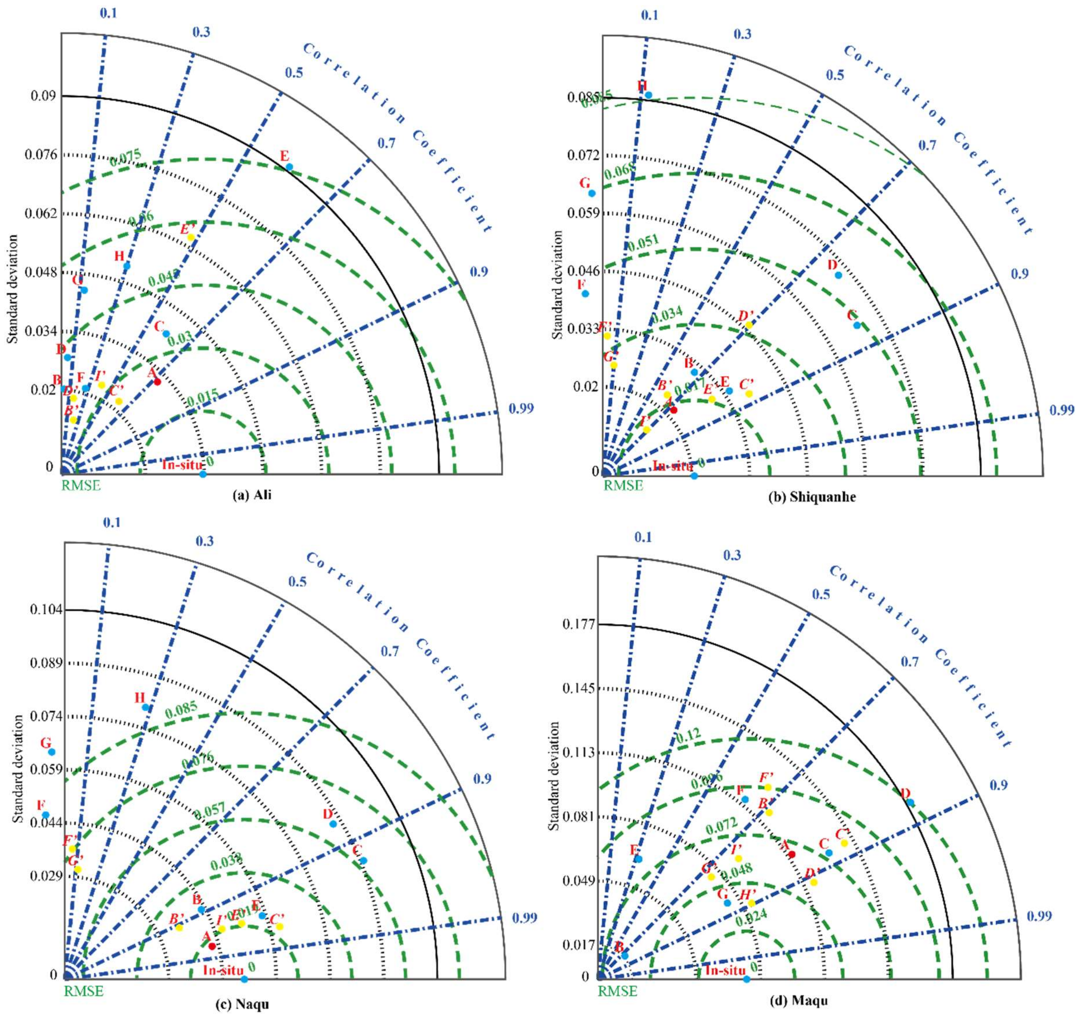
The homogenized and merged product presents SSM with global coverage and spatial resolution of 0.25°. The time length of the product spans the entire Product Period covered by different sensors, i.e., 2007–2016. The blended SSM data were compared with different SSM products over the Product Period while using the Taylor diagrams in Figure 8. The Taylor diagram represents the correlation coefficient, the centred unbiased root mean square difference, and the standard deviation while using a two-dimensional plot [48]. The in-situ measurements of Tibet-Obs networks (Naqu, Maqu, Ali, and Shiquanhe) were served as the reference. The original SSM products in Figure 8 include SMOS (B), AMSR2 (C), SMAP (D), ERA-Interim (E), merged PASSIVE (F), ESA-CCI merged ACTIVE (G), and their corresponding scaled data (B, C, D, E, F, G) after climatology scaling. Furthermore, an arithmetic average was calculated to obtain the average value of both original data and scaled data. The product I is the simple average of scaled data and Product H is a simple average of the original data.
Comparing the blended SSM results in this research (A) with other SSM product (B, C, D, E). In the Ali network (Figure 8a), the blended SSM shows a better quality than SMOS and ERA-Interim SSM products and it has a similar RMSE and standard deviation and a higher correlation coefficient with AMSR2 and SMAP products. In the Shiquanhe and Naqu network (Figure 8b,c), the blended SSM gives a better estimation than all of these products. In Maqu network (Figure 8d), the blended SSM show a better estimation than AMSR2 and SMAP SSM product, but SMOS and ERA-Interim show lower standard deviation. However, the correlation coefficients are similar.
When comparing the simple average of original data (H) with the simple average of scaled data (I), the I data performs much better in arid and semi-arid regions with a low standard deviation, and root mean squares. It that means a climatology scaling is needed before merging and CDF matching. Comparing the simple average of scaled data (I) with the blended SSM data (A), it shows that the least-squares method performs better than arithmetic averaging in Ali and SQ networks, which gives a better result close to the in-situ measured data with a similar correlation coefficient and root mean squares (Figure 8a,b). Although they perform similar well in Maqu Figure 8d, it was still verified that the least-squares method is needed and performed better in the arid areas over the Tibetan Plateau.
The merged PASSIVE (F), merged ACTIVE data (G), original satellites data SMOS (B), AMSR2 (C), SMAP (D), and ERA-Interim (E) have higher standard deviations before climatology scaling. The more significant standard deviation indicates more fluctuations, especially for PASSIVE and ACTIVE. After a scaling based on the in-situ climatology, the standard deviation of them became smaller. It is one of the reasons why a climatology scaling is needed before a merging step. It is essential to eliminate the systematic difference between the different datasets before further merging can be performed.
The PASSIVE and ACTIVE products did not perform well before climatology scaling, while SMOS and AMSR2 performed well in most of the conditions. The SMOS data accurately estimated SSM and captured the in-situ SSM dynamics. Especially in the Shiquanhe and Naqu network (Figure 8b,c), it performs similarly to the blended SSM data. When comparing PASSIVE with ACTIVE, the scaled ACTIVE performs better, which means that the average weight of ACTIVE is greater than the weight of PASSIVE in the Blended product.
4.2. RZSM Product
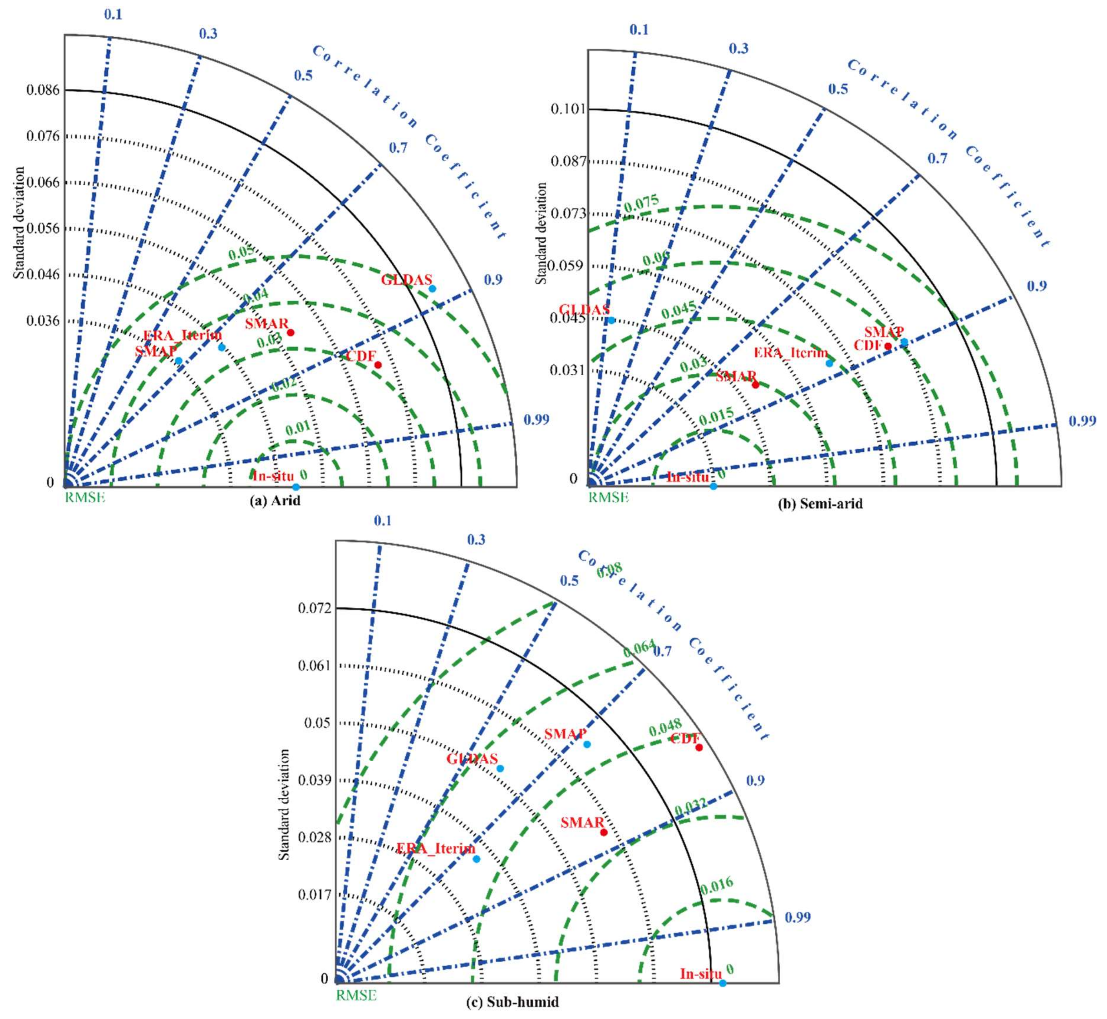
The inter-comparison of RZSM products is a comparison between the RZSM products that were generated in this research (e.g., RZSM product from CDF matching and SMAR model) and other products (e.g., ERA-Interim RZSM data, GLDAS RZSM data, and SMAP L4 RZSM data) over the one-year validation period, when the RZSM measurements were available. The first RZSM product (presented with the tag “CDF” and red dots in Figure 9) was generated while using CDF Matching based on in-situ SM measurements. The other RZSM product (presented with the tag “SMAR” and red dots in Figure 9) was generated using the SMAR model. The other RZSM data ERA-Interim, GLDAS, and SMAP were presented with cyan dots in Figure 9.
In different climate zones, each RZSM product shows different characteristics. In the sub-humid region (Figure 9c), the SMAR product shows a lower standard deviation (0.058) when compared with CDF product (0.080), and it also shows a slightly lower root mean square error (0.037 vs. 0.047) and similar correlation coefficient (0.85 vs 0.81). Both methods of deriving RZSM are satisfactory when compared with in-situ measurements. Both are better than the GLDAS product refers to RMSE and standard deviation. Additionally, both are similar or slightly better than SMAP L4 product and ERA-Interim RZSM product refers to RMSE and correlation coefficient. In the semi-arid climate zone (Figure 9b), the SMAR model performs much better when compared with other products with a low standard deviation (0.049) and root mean square error (0.03). The relatively unsatisfactory performances of CDF matching may due to the SM dynamics of semi-arid region, as suggested Manfreda et al. (2007) [54]. The relationship between SSM and RZSM is more complicated, and the two variables are more likely to be decoupled in such regions. As such, a physically-based estimation (e.g., SMAR model) can be better than a simple depth scaling method [24,55]. When compared with other products, the SMAR model gives a better estimation than ERA-Interim, and SMAP RZSM product, and a lower RMSE than GLDAS RZSM product. The CDF method gives a better estimation than SMAP RZSM product and a higher correlation coefficient than the others. In the arid region (Figure 9a), the SMAR product and CDF product both show a mediocre performance, which might be due to the low availability of in-situ RZSM data in the arid region, as both of the methods rely on the dynamics of in-situ RZSM time series. Nevertheless, using SMAR model and CDF Matching to generate the RZSM is reliable and straightforward, which can give a robust prediction of RZSM from satellite SSM.
It is worth to note that the relationship between SSM and RZSM is obtained while using zonally averaged data, which ignored some specific difference between different stations or different soil layers. For example, the 40cm soil moisture of some stations in Shiquanhe networks are extremely low, and the seasonal change is small, while, in another station of the same network, it is incredibly high and fluctuates wildly.
5. Conclusions
In this study, performing satellite data merging, climatology scaling, SSM data blending, and depth scaling produced consistent SSM and RZSM products. As discussed above, these procedures composed an integrated method to study SSM and RZSM using the sparse in-situ measurement networks over Tibetan Plateau. First, different satellites observed data were merged into two satellites-based products (i.e., ACTIVE and PASSIVE). Subsequently, the satellite products were constrained by in-situ measurements using CDF matching and the in-situ scaled land surface model-simulated data. Next, all of the input data were merged into a consistent SSM product. Last, the SSM product was scaled while using CDF matching to obtain the RZSM. Furthermore, an analytical model SMAR was also applied to enable a physically based estimation of RZSM.
Beyond the typical data blending research, this research constrained the blending data sets with the in-situ climatology [2]. It can eliminate the influence by using different land surface model simulations. It should be noticed that the choice of the climate classification method could also influence the in-situ climatology. Nevertheless, the generated consistent SSM and RZSM products captured the in-situ dynamics.
The methods for generating RZSM products are CDF matching and the SMAR model, which are recommended due to their simplicities and reliable performances. Both of them are an economical and efficient method for maximizing the use of limited in-situ measured data. The calibration of them can work while using a two-year coarse resolution in-situ RZSM measurement. The predicted RZSM products from the blended SSM product can follow the in-situ measurement reasonably well. The high correlation between RZSM products and in-situ measured RZSM and low uncertainties indicate that the CDF Matching and SMAR model can give a robust RZSM prediction. Nevertheless, the RZSM states and data availability vary from region to region. For example, the SMAR model performs well as a physical-based model in the semi-arid region, while CDF Matching performs slightly better in the arid region.
Author Contributions
Conceptualization, R.Z., and Y.Z.; methodology, R.Z., Y.Z. and S.M.; software, R.Z., Y.Z. and S.M.; validation, R.Z.; formal analysis, R.Z.; investigation, R.Z., Y.Z. and Z.S.; resources, Y.Z., Z.S. and S.M.; data curation, R.Z.; writing—original draft preparation, R.Z.; writing—review and editing, R.Z., Y.Z. and S.M.; visualization, R.Z.; supervision, Y.Z., S.M., and Z.S.; project administration, Y.Z., Z.S., and S.M.; funding acquisition, Y.Z., Z.S. and S.M. All authors have read and agreed to the published version of the manuscript.
Funding
This research was funded by the University of Twente, based on “the MSc Thesis Excellence Programme” and the University of Basilicata, with “PhD scholarship”; supported by Water JPI project “An integrative information aqueduct to close the gaps between global satellite observation of water cycle and local sustainable management of water resources (iAqueduct)”; by the COST Action CA16219 “HARMONIOUS—Harmonization of UAS techniques for agricultural and natural ecosystems monitoring” and by the National Natural Science Foundation of China (grant no. 41971033).
Conflicts of Interest
The authors declare no conflict of interest.
References
- Su, Z.; Wen, J.; Dente, L.; van der Velde, R.; Wang, L.; Ma, Y.; Yang, K.; Hu, Z. The Tibetan Plateau observatory of plateau scale soil moisture and soil temperature (Tibet-Obs) for quantifying uncertainties in coarse resolution satellite and model products. Hydrol. Earth Syst. Sci. 2011, 15, 2303–2316. [Google Scholar] [CrossRef] [Green Version]
- Zeng, Y.; Su, Z.; Van Der Velde, R.; Wang, L.; Xu, K.; Wang, X.; Wen, J. Blending satellite observed, model simulated, and in situ measured soil moisture over Tibetan Plateau. Remote Sens. 2016, 8, 268. [Google Scholar] [CrossRef] [Green Version]
- Taylor, C.M.; de Jeu, R.A.M.; Guichard, F.; Harris, P.P.; Dorigo, W.A. Afternoon rain more likely over drier soils. Nature 2012, 489, 423–426. [Google Scholar] [CrossRef] [PubMed] [Green Version]
- Reynolds, C.A.; Jackson, T.J.; Rawls, W.J. Estimating soil water-holding capacities by linking the Food and Agriculture Organization soil map of the world with global pedon databases and continuous pedotransfer functions. Water Resour. Res. 2000, 36, 3653–3662. [Google Scholar] [CrossRef]
- Drusch, M.; Viterbo, P. Assimilation of Screen-Level Variables in ECMWF’s Integrated Forecast System: A Study on the Impact on the Forecast Quality and Analyzed Soil Moisture. Mon. Weather Rev. 2007, 135, 300–314. [Google Scholar] [CrossRef]
- Ma, Y.; Ma, W.; Zhong, L.; Hu, Z.; Li, M.; Zhu, Z.; Han, C.; Wang, B.; Liu, X. Monitoring and Modeling the Tibetan Plateau’s climate system and its impact on East Asia. Sci. Rep. 2017, 7, 1–6. [Google Scholar] [CrossRef] [Green Version]
- Bengtsson, L. The global atmospheric water cycle. Environ. Res. Lett. 2010, 5, 1–8. [Google Scholar] [CrossRef]
- Yang, K.; Wu, H.; Qin, J.; Lin, C.; Tang, W.; Chen, Y. Recent climate changes over the Tibetan Plateau and their impacts on energy and water cycle: A review. Glob. Planet. Chang. 2014, 112, 79–91. [Google Scholar] [CrossRef]
- Su, Z.; De Rosnay, P.; Wen, J.; Wang, L.; Zeng, Y. Evaluation of ECMWF’s soil moisture analyses using observations on the Tibetan Plateau. J. Geophys. Res. Atmos. 2013, 118, 5304–5318. [Google Scholar] [CrossRef] [Green Version]
- Zhao, H.; Zeng, Y.; Lv, S.; Su, Z. Analysis of Soil Hydraulic and Thermal Properties for Land Surface Modelling over the Tibetan Plateau. Earth Syst. Sci. Data 2018, 10, 1031–1061. [Google Scholar] [CrossRef] [Green Version]
- Ma, Y.; Kang, S.; Zhu, L.; Xu, B.; Tian, L.; Yao, T. Roof of the World: Tibetan observation and research platform. Bull. Am. Meteorol. Soc. 2008, 89, 1487–1492. [Google Scholar]
- Yang, K.; Qin, J. A Multiscale Soil Moisture and Freeze–Thaw Monitoring Network on the Third Pole. Bull. Am. Meteorol. Soc. 2013, 94, 1907–1916. [Google Scholar] [CrossRef]
- Kerr, Y.H.; Waldteufel, P.; Wigneron, J.-P.; Berger, M.; Martinuzzi, J.-M.; Font, J. Soil moisture retrieval from space: The Soil Moisture and Ocean Salinity (SMOS) mission. IEEE Trans. Geosci. Remote Sens. 2001, 39, 1729–1735. [Google Scholar] [CrossRef]
- Entekhabi, D.; Njoku, E.G.; O’Neill, P.E.; Kellogg, K.H.; Crow, W.T.; Edelstein, W.N.; Entin, J.K.; Goodman, S.D.; Jackson, T.J.; Johnson, J.; et al. The Soil Moisture Active Passive (SMAP) Mission. Proc. IEEE 2010, 98, 704–716. [Google Scholar] [CrossRef]
- Owe, M.; de Jeu, R.; Holmes, T. Multisensor historical climatology of satellite-derived global land surface moisture. J. Geophys. Res. Earth Surf. 2008, 113, 1–17. [Google Scholar] [CrossRef]
- Wagner, W.; Hahn, S.; Kidd, R.; Melzer, T.; Bartalis, Z.; Hasenauer, S.; Figa-Saldaña, J.; De Rosnay, P.; Jann, A.; Schneider, S.; et al. The ASCAT soil moisture product: A review of its specifications, validation results, and emerging applications. Meteorol. Z. 2013, 22, 5–33. [Google Scholar] [CrossRef] [Green Version]
- Dee, D.P.; Uppala, S.M.; Simmons, A.J.; Berrisford, P.; Poli, P.; Kobayashi, S.; Andrae, U.; Balmaseda, M.A.; Balsamo, G.; Bauer, P.; et al. The ERA-Interim reanalysis: Configuration and performance of the data assimilation system. Q. J. R. Meteorol. Soc. 2011, 137, 553–597. [Google Scholar] [CrossRef]
- Balsamo, G.; Albergel, C.; Beljaars, A.; Boussetta, S.; Brun, E.; Cloke, H.; Dee, D.; Dutra, E.; Munõz-Sabater, J.; Pappenberger, F.; et al. ERA-Interim/Land: A global land surface reanalysis data set. Hydrol. Earth Syst. Sci. 2015, 19, 389–407. [Google Scholar] [CrossRef] [Green Version]
- Rodell, M.; Houser, P.R.; Jambor, U.; Gottschalck, J.; Mitchell, K.; Meng, C.-J.; Arsenault, K.; Cosgrove, B.; Radakovich, J.; Bosilovich, M.; et al. The Global Land Data Assimilation System. Bull. Am. Meteorol. Soc. 2004, 85, 381–394. [Google Scholar] [CrossRef] [Green Version]
- Wagner, W.; Dorigo, W.; De Jeu, R.; Fernandez, D.; Benveniste, J.; Haas, E.; Ertl, M. Fushion of ACTIVE and PASSIVE Microwave Observations to Create an Essential Climate Variable Data Record on Soil Moisture. ISPRS Ann. Photogramm. Remote Sens. Spat. Inf. Sci. 2012, 7, 315–321. [Google Scholar]
- Dorigo, W.A.; Gruber, A.; De Jeu, R.A.M.; Wagner, W.; Stacke, T.; Loew, A.; Albergel, C.; Brocca, L.; Chung, D.; Parinussa, R.M.; et al. Evaluation of the ESA CCI soil moisture product using ground-based observations. Remote Sens. Environ. 2015, 162, 380–395. [Google Scholar] [CrossRef]
- Zhan, X.; Liu, J.; Zhao, L. Soil Moisture Operational Product System (SMOPS) Algorithm Theretical Basis Document. Available online: https://www.ospo.noaa.gov/Products/land/smops/algo.html (accessed on 17 August 2016).
- Naeimi, V.; Scipal, K.; Bartalis, Z.; Hasenauer, S.; Wagner, W. An improved soil moisture retrieval algorithm for ERS and METOP scatterometer observations. IEEE Trans. Geosci. Remote Sens. 2009, 47, 1999–2013. [Google Scholar] [CrossRef]
- Manfreda, S.; Brocca, L.; Moramarco, T.; Melone, F.; Sheffield, J. A physically based approach for the estimation of root-zone soil moisture from surface measurements. Hydrol. Earth Syst. Sci. 2014, 18, 1199–1212. [Google Scholar] [CrossRef] [Green Version]
- Gao, X.; Wu, P.; Zhao, X.; Zhou, X.; Zhang, B.; Shi, Y.; Wang, J. Estimating soil moisture in gullies from adjacent upland measurements through different observation operators. J. Hydrol. 2013, 486, 420–429. [Google Scholar] [CrossRef]
- Han, E.; Merwade, V.; Heathman, G.C. Application of data assimilation with the Root Zone Water Quality Model for soil moisture profile estimation in the upper Cedar Creek, Indiana. Hydrol. Process. 2012, 26, 1707–1719. [Google Scholar] [CrossRef]
- Reichle, R.H.; Liu, Q.; Koster, R.D.; Crow, W.T.; De Lannoy, G.J.M.; Kimball, J.S.; Ardizzone, J.V.; Bosch, D.; Colliander, A.; Cosh, M.; et al. Version 4 of the SMAP Level-4 Soil Moisture Algorithm and Data Product. J. Adv. Model. Earth Syst. 2019, 11, 3106–3130. [Google Scholar] [CrossRef] [Green Version]
- Brocca, L.; Melone, F.; Moramarco, T.; Wagner, W.; Albergel, C. Scaling and Filtering Approaches for the Use of Satellite Soil Moisture Observations. In Remote Sensing of Energy Fluxes and Soil Moisture Content; CRC Press: Boca Raton, FL, USA, 2013; pp. 411–426. ISBN 978-1-4665-0578-0. [Google Scholar]
- Baldwin, D.; Manfreda, S.; Lin, H.; Smithwick, E.A.H. Estimating Root Zone Soil Moisture Across the Eastern United States with Passive Microwave Satellite Data and a Simple Hydrologic Model. Remote Sens. 2019, 11, 2013. [Google Scholar] [CrossRef] [Green Version]
- Gao, X.; Zhao, X.; Brocca, L.; Huo, G.; Lv, T.; Wu, P. Depth scaling of soil moisture content from surface to profile: Multistation testing of observation operators. Hydrol. Earth Syst. Sci. Discuss. 2017, 292, 1–25. [Google Scholar] [CrossRef]
- Reichle, R.H.; Koster, R.D. Bias reduction in short records of satellite soil moisture. Geophys. Res. Lett. 2004, 31, 2–5. [Google Scholar] [CrossRef] [Green Version]
- Drusch, M. Observation operators for the direct assimilation of TRMM microwave imager retrieved soil moisture. Geophys. Res. Lett. 2005, 32, L15403. [Google Scholar] [CrossRef]
- Liu, Y.Y.; Parinussa, R.M.; Dorigo, W.A.; De Jeu, R.A.M.; Wagner, W.M.; Van Dijk, A.I.J.; McCabe, M.F.; Evans, J.P. Developing an improved soil moisture dataset by blending passive and active microwave satellite-based retrievals. Hydrol. Earth Syst. Sci. 2011, 15, 425–436. [Google Scholar] [CrossRef] [Green Version]
- Bankman, I.N. Handbook of Medical Image Processing and Analysis; Bronzino, J., Ed.; Elsevier/Academic Press: Amsterdam, The Netherlands, 2009; ISBN 9780123739049. [Google Scholar]
- Njoku, E.G.; Jackson, T.J.; Lakshmi, V.; Chan, T.K.; Nghiem, S.V. Soil moisture retrieval from AMSR-E. IEEE Trans. Geosci. Remote Sens. 2003, 41, 215–228. [Google Scholar] [CrossRef]
- Njoku, E.G.; Ashcroft, P.; Chan, T.K.; Li, L. Global survey and statistics of radio-frequency interference in AMSR-E land observations. IEEE Trans. Geosci. Remote Sens. 2005, 43, 938–946. [Google Scholar] [CrossRef]
- Njoku, E.G.; Chan, S.K. Vegetation and surface roughness effects on AMSR-E land observations. Remote Sens. Environ. 2006, 100, 190–199. [Google Scholar] [CrossRef]
- Imaoka, K.; Kachi, M.; Fujii, H.; Murakami, H.; Hori, M.; Ono, A.; Igarashi, T.; Nakagawa, K.; Oki, T.; Honda, Y.; et al. Global change observation mission (GCOM) for monitoring carbon, water cycles, and climate change. Proc. IEEE 2010, 98, 717–734. [Google Scholar] [CrossRef]
- Imaoka, K.; Maeda, T.; Kachi, M.; Kasahara, M.; Ito, N.; Nakagawa, K. Status of AMSR2 Instrument on GCOM-W1. Earth Observing Missions and Sensors: Development, Implementation, and Characterization II; Shimoda, H., Xiong, X., Cao, C., Gu, X., Kim, C., Kiran Kumar, A.S., Eds.; SPIE Asia-Pacific Remote Sensing: Kyoto, Japan, 2012; Volume 852815, pp. 1–6. [Google Scholar]
- Kerr, Y.H.; Waldteufel, P.; Richaume, P.; Wigneron, J.P.; Ferrazzoli, P.; Mahmoodi, A.; Al Bitar, A.; Cabot, F.; Gruhier, C.; Juglea, S.E.; et al. The SMOS Soil Moisture Retrieval Algorithm. Geosci. Remote Sens. 2012, 50, 1384–1403. [Google Scholar] [CrossRef]
- Wigneron, J.P.; Kerr, Y.H.; Waldteufel, P.; Saleh, K.; Escorihuela, M.J.; Richaume, P.; Ferrazzoli, P.; de Rosnay, P.; Gurney, R.; Calvet, J.C.; et al. L-band Microwave Emission of the Biosphere (L-MEB) Model: Description and calibration against experimental data sets over crop fields. Remote Sens. Environ. 2007, 107, 639–655. [Google Scholar] [CrossRef]
- Zeng, J.; Li, Z.; Chen, Q.; Bi, H.; Qiu, J.; Zou, P. Evaluation of remotely sensed and reanalysis soil moisture products over the Tibetan Plateau using in-situ observations. Remote Sens. Environ. 2015, 163, 91–110. [Google Scholar] [CrossRef]
- Colliander, A.; Jackson, T.J.; Bindlish, R.; Chan, S.; Das, N.; Kim, S.B.; Cosh, M.H.; Dunbar, R.S.; Dang, L.; Pashaian, L.; et al. Validation of SMAP surface soil moisture products with core validation sites. Remote Sens. Environ. 2017, 191, 215–231. [Google Scholar] [CrossRef]
- Gruber, A.; Dorigo, W.A.; Crow, W.; Wagner, W. Triple Collocation-Based Merging of Satellite Soil Moisture Retrievals. IEEE Trans. Geosci. Remote Sens. 2017, 55, 6780–6792. [Google Scholar] [CrossRef]
- Gruber, A.; Scanlon, T.; Van Der Schalie, R.; Wagner, W.; Dorigo, W. Evolution of the ESA CCI Soil Moisture climate data records and their underlying merging methodology. Earth Syst. Sci. Data 2019, 11, 717–739. [Google Scholar] [CrossRef] [Green Version]
- Dorigo, W.; Wagner, W.; Albergel, C.; Albrecht, F.; Balsamo, G.; Brocca, L.; Chung, D.; Ertl, M.; Forkel, M.; Gruber, A.; et al. ESA CCI Soil Moisture for improved Earth system understanding: State-of-the art and future directions. Remote Sens. Environ. 2017, 203, 185–215. [Google Scholar] [CrossRef]
- Saxton, K.E.; Rawls, W.J. Soil Water Characteristic Estimates by Texture and Organic Matter for Hydrologic Solutions. Soil Sci. Soc. Am. J. 2006, 70, 1569. [Google Scholar] [CrossRef] [Green Version]
- Petropoulos, G.P. Remote Sensing of Energy Fluxes and Soil Moisture Content; CRC Press: Boca Raton, FL, USA, 2017; ISBN 9781138077577. [Google Scholar]
- Brocca, L.; Hasenauer, S.; Lacava, T.; Melone, F.; Moramarco, T.; Wagner, W.; Dorigo, W.; Matgen, P.; Martínez-Fernández, J.; Llorens, P.; et al. Soil moisture estimation through ASCAT and AMSR-E sensors: An intercomparison and validation study across Europe. Remote Sens. Environ. 2011, 115, 3390–3408. [Google Scholar] [CrossRef]
- Yilmaz, M.T.; Crow, W.T.; Anderson, M.C.; Hain, C. An objective methodology for merging satellite- and model-based soil moisture products. Water Resour. Res. 2012, 48, 1–15. [Google Scholar] [CrossRef]
- Stoffelen, A. Toward the true near-surface wind speed: Error modeling and calibration using triple collocation. J. Geophys. Res. Ocean. 1998, 103, 7755–7766. [Google Scholar] [CrossRef]
- Baldwin, D.; Manfreda, S.; Keller, K.; Smithwick, E.A.H. Predicting root zone soil moisture with soil properties and satellite near-surface moisture data across the conterminous United States. J. Hydrol. 2017, 546, 393–404. [Google Scholar] [CrossRef]
- Dorigo, W.A.; Scipal, K.; Parinussa, R.M.; Liu, Y.Y.; Wagner, W.; De Jeu, R.A.M.; Naeimi, V. Error characterisation of global active and passive microwave soil moisture datasets. Hydrol. Earth Syst. Sci. 2010, 14, 2605–2616. [Google Scholar] [CrossRef] [Green Version]
- Zwieback, S.; Scipal, K.; Dorigo, W.; Wagner, W. Structural and statistical properties of the collocation technique for error characterization. Nonlinear Process. Geophys. 2012, 19, 69–80. [Google Scholar] [CrossRef]
- Manfreda, S.; McCabe, M.F.; Fiorentino, M.; Rodríguez-Iturbe, I.; Wood, E.F. Scaling characteristics of spatial patterns of soil moisture from distributed modelling. Adv. Water Resour. 2007, 30, 2145–2150. [Google Scholar] [CrossRef]
Figure 1.
Tibetan Plateau Location in the World Map and In-situ Measurement Networks Distribution over Study Area.
Figure 1.
Tibetan Plateau Location in the World Map and In-situ Measurement Networks Distribution over Study Area.

Figure 2.
Methodology Flowchart of SSM and root zone soil moisture (RZSM) data prediction.

Figure 3.
Time Series of Data Involved in Data Merging Procedure (a) Original Satellites Data, Scaled Data used for Merging, European Space Agency Climate Change Initiative (ESA-CCI) PASSIVE Data used for comparison and Merged PASSIVE SM Product (an example of the arid region) (b) Partial time series from 1-March-2010 to 1-March-2012; and, (c) Partial time-series from 1-March-2015 to 1-September-2016.

Figure 4.
Time-longitude Diagrams of surface soil moisture (SSM) products: (a) In-situ data over the Calibration Period; (b) the Cumulative Distribution Function (CDF) matching example at the location of the in-situ station of sub-humid region; (c) scaled European Centre for Medium-Range Weather Forecasts (ERA)-Interim data; and, (d) original ERA-Interim data over the Product Period.

Figure 5.
Time Series Diagrams of original PASSIVE product, original ACTIVE product, Scaled PASSIVE product, scaled ACTIVE product, Blended SSM product, in-situ Tibet-Obs product, and ESA-CCI SSM product. (A zonally averaged data over Sub-humid region).
Figure 5.
Time Series Diagrams of original PASSIVE product, original ACTIVE product, Scaled PASSIVE product, scaled ACTIVE product, Blended SSM product, in-situ Tibet-Obs product, and ESA-CCI SSM product. (A zonally averaged data over Sub-humid region).

Figure 6.
Optimal Weights Distribution of SM Products for Blending: (a) Scaled ERA-Interim (in average 0.30); (b) Scaled PASSIVE (in average 0.14); and, (c) Scaled ACTIVE (in average 0.60).
Figure 6.
Optimal Weights Distribution of SM Products for Blending: (a) Scaled ERA-Interim (in average 0.30); (b) Scaled PASSIVE (in average 0.14); and, (c) Scaled ACTIVE (in average 0.60).

Figure 7.
Tibet-Obs In-situ SSM and RZSM Data over Calibration Period: (a) Semiarid region; (b) Sub-humid region.
Figure 7.
Tibet-Obs In-situ SSM and RZSM Data over Calibration Period: (a) Semiarid region; (b) Sub-humid region.

Figure 8.
Taylor Diagrams of Inter-comparison between Blended Data and Others: (a) Ali; (b) Shiquanhe; (c) Naqu; (d) Maqu; A with red dot represents the blended SSM product; B, C, D, E, F with cyan dots represent the original SSM products SMOS, AMSR2, SMAP, ERA-Interim, merged PASSIVE, ESA-CCI merged ACTIVE; B, C, D, E, F with yellow dots represent the in-situ climatology scaled SSM data; H and I represent a simple averaged of original products and a simple average of scaled products.

Figure 9.
Taylor Diagrams of Inter-comparison between RZSM Data and Others: (a) Arid; (b) Semi-arid; and, (c) Sub-humid; Products name tags with red dots represents the predicted RZSM product from this research; Cyan dots represent ERA-Interim, GLDAS, and SMAP RZSM products.
Figure 9.
Taylor Diagrams of Inter-comparison between RZSM Data and Others: (a) Arid; (b) Semi-arid; and, (c) Sub-humid; Products name tags with red dots represents the predicted RZSM product from this research; Cyan dots represent ERA-Interim, GLDAS, and SMAP RZSM products.


Table 1.
Start-End Dates Diagram of all the Data Sets for Data Processing.
| Data Sources | Datasets | Covered Time Range | Spatial and Temporal Resolution |
|---|---|---|---|
| In-situ Measurements | Tibet-Obs | 1-September-2013 to 31-August-2015 | Point; Every 15 min |
| 1-September-2015 to 31-August-2016 | |||
| Land Data Assimilation | ERA-Interim | 1-January-2007 to 31-December-2016 | 25 km; Daily |
| GLDAS | 1-September-2015 to 31-August-2016 | 25 km; Daily | |
| Satellites Observations (PASSIVE) | AMSRE | 1-January-2007 to 3-October-2011 | 25 km; Daily |
| SMOS | 1-June-2010 to 31-December-2016 | 30 km; Daily | |
| AMSR2 | 3-July-2012 to 31-December-2016 | 25 km; Daily | |
| SMAP | 31-March-2015 to 31-December-2016 | 36 km; Daily | |
| ESA-CCI PASSIVE | 1-January-2007 to 31-December-2016 | 25 km; Daily | |
| Satellites Observations (ACTIVE) | ESA-CCI ACTIVE | 1-January-2007 to 31-December-2016 | 25 km; Daily |
| Blended Product | ESA-CCI Soil Moisture | 1-January-2007 to 31-December-2016 | 25 km; Daily |
Table 2.
Summary of the relative errors and optimal weights (averaged values over the entire study area) used in satellites data merging.
Table 2.
Summary of the relative errors and optimal weights (averaged values over the entire study area) used in satellites data merging.
| Merging Period | Date | ||
|---|---|---|---|
| S1 | 1-June-2007 to 31-May-2010 | = 0.0023 | = 1 |
| S2 | 1-June-2010 to 3-October-2011 | = 0.0031 | = 0.613 |
| = 0.0068 | = 0.387 | ||
| S3 | 4-October-2011 to 2-July-2012 | = 0.0061 | = 1 |
| S4 | 3-July-2012 to 30-March-2015 | = 0.0085 | = 0.431 |
| = 0.0057 | = 0.569 | ||
| S5 | 31-March-2015 to 31-December-2016 | = 0.0074 | = 0.313 |
| = 0.0047 | = 0.395 | ||
| = 0.0065 | = 0.292 |
Table 3.
Summary of the results of the calibration with the SMAR methods.
| Climate Zone | RMSE | ||||
|---|---|---|---|---|---|
| ARID: Ali | 0.0505 | 0.4967 | 0.3343 | 0.5020 | 0.0436 |
| SEMI-ARID: Naqu | 0.0230 | 0.1238 | 0.1987 | 0.1754 | 0.0274 |
| SUB-HUMID: Maqu | 0.0680 | 0.0602 | 0.0648 | 0.2582 | 0.0367 |
© 2020 by the authors. Licensee MDPI, Basel, Switzerland. This article is an open access article distributed under the terms and conditions of the Creative Commons Attribution (CC BY) license (http://creativecommons.org/licenses/by/4.0/).
Share and Cite
MDPI and ACS Style
Zhuang, R.; Zeng, Y.; Manfreda, S.; Su, Z. Quantifying Long-Term Land Surface and Root Zone Soil Moisture over Tibetan Plateau. Remote Sens. 2020, 12, 509. https://0-doi-org.brum.beds.ac.uk/10.3390/rs12030509
AMA Style
Zhuang R, Zeng Y, Manfreda S, Su Z. Quantifying Long-Term Land Surface and Root Zone Soil Moisture over Tibetan Plateau. Remote Sensing. 2020; 12(3):509. https://0-doi-org.brum.beds.ac.uk/10.3390/rs12030509
Chicago/Turabian StyleZhuang, Ruodan, Yijian Zeng, Salvatore Manfreda, and Zhongbo Su. 2020. "Quantifying Long-Term Land Surface and Root Zone Soil Moisture over Tibetan Plateau" Remote Sensing 12, no. 3: 509. https://0-doi-org.brum.beds.ac.uk/10.3390/rs12030509
Note that from the first issue of 2016, this journal uses article numbers instead of page numbers. See further details here.