Article

Comparison of Support Vector Machine and Random Forest Algorithms for Invasive and Expansive Species Classification Using Airborne Hyperspectral Data

Department of Geoinformatics, Faculty of Geography and Regional Studies, University of Warsaw, Cartography and Remote Sensing, ul. Krakowskie Przedmieście 30, 00-927 Warsaw, Poland
*
Author to whom correspondence should be addressed.
Submission received: 17 December 2019 / Revised: 29 January 2020 / Accepted: 3 February 2020 / Published: 5 February 2020
(This article belongs to the Special Issue Hyperspectral Remote Sensing of Agriculture and Vegetation)

Abstract

:
Invasive and expansive plant species are considered a threat to natural biodiversity because of their high adaptability and low habitat requirements. Species investigated in this research, including Solidago spp., Calamagrostis epigejos, and Rubus spp., are successfully displacing native vegetation and claiming new areas, which in turn severely decreases natural ecosystem richness, as they rapidly encroach on protected areas (e.g., Natura 2000 habitats). Because of the damage caused, the European Union (EU) has committed all its member countries to monitor biodiversity. In this paper we compared two machine learning algorithms, Support Vector Machine (SVM) and Random Forest (RF), to identify Solidago spp., Calamagrostis epigejos, and Rubus spp. on HySpex hyperspectral aerial images. SVM and RF are reliable and well-known classifiers that achieve satisfactory results in the literature. Data sets containing 30, 50, 100, 200, and 300 pixels per class in the training data set were used to train SVM and RF classifiers. The classifications were performed on 430-spectral bands and on the most informative 30 bands extracted using the Minimum Noise Fraction (MNF) transformation. As a result, maps of the spatial distribution of analyzed species were achieved; high accuracies were observed for all data sets and classifiers (an average F1 score above 0.78). The highest accuracies were obtained using 30 MNF bands and 300 sample pixels per class in the training data set (average F1 score > 0.9). Lower training data set sample sizes resulted in decreased average F1 scores, up to 13 percentage points in the case of 30-pixel samples per class.

Graphical Abstract

1. Introduction

The spread of invasive and expansive species is one of the main threats to biodiversity and functioning of ecosystems [1]. This results in transformation of natural habitats, displacement of native species, and degrading environmental conditions (e.g., number of existing micro- and macrophytes). It also generates economic losses by degrading the quality of soil and destroying road and railway infrastructure [2]. In the European Union (EU), it is estimated that the cost of controlling and combating invasive species amounts to approximately 12 billion EUR per year [3]. Implementation of appropriate remedial strategies and effective limitation of the invasion’s effects require constant monitoring, which is emphasized in the EU Regulation No. 1143/2014.
The species that pose a threat to natural habitats protected under the Natura 2000 program in Poland include, for example, native expansive plants such as blackberry shrubs (Rubus spp. L.), perennial wood small-reed (Calamagrostis epigejos (L.) Roth), and foreign invasive goldenrod species (Solidago spp. L). These species do not have high requirements concerning their habitat; they also reproduce quickly, both in terms of vegetative and generative reproduction, and they stifle other plants [4]. They negatively impact valuable natural habitats, such as inland sand calcareous grasslands, mountain and lowland Nardus grasslands, Molinia meadows, and alluvial meadows. They are extensively used in fresh low pastures in mountain hay and bent-grass meadows [5,6,7]. In order to prevent further changes in the vegetation, these harmful species should be identified and removed preferably at the early stages of invasion.
The current monitoring of plant species changes is based on fixed target areas. Individual specimens of the species found in target areas are counted, and the observed regularities are extrapolated to the whole area, which can differentiate due to, for example, environmental components or land use. In comparison to traditional fields, remote sensing allows for objective and repetitive monitoring that can be conducted both on local and global scales [8,9]. Considering the complexity of class distinctions, both intra-class similarities and differences between classes, the data which can be used for this purpose are multispectral, such as Landsat [10], WorldView-2 [11], or hyperspectral data (e.g., HyMap) [12]. As hyperspectral data constitute a source of ongoing information about spectral reflection, they provide a lot of information about the biophysical and chemical characteristics of the analyzed vegetation [13,14,15]. Either hyperspectral satellite data (e.g., Hyperion [16] and CHRIS [15,17]) or aerial data (e.g., APEX [18] and AISA [19,20]) are used, depending on the size of the research area and the canopy characteristics of the identified vegetation. Airborne data are more useful for the detection of small, less compact patches of plant species because of their high spatial resolution [16]. The study of Mediterranean plants in southern France confirms that spectral and spatial resolution influence the accuracy of vegetation mapping [21]. The highest accuracy of classification of five vegetation types was obtained using the airborne hyperspectral imaging sensor, HyMap. Depending on the classification method used, the overall accuracies (OAs) ranged from 62.3% for k-nearest neighbor (k-nn), 67.7% for Random Forest (RF), and 70.2% for Support Vector Machine (SVM), up to 72.5% for Artificial Neural Networks (ANNs), while the use of ASTER satellite data resulted in slightly lower accuracy levels (from 60.3%), and the worst results were obtained using multispectral data Landsat 7 ETM + (59.3%).
Multi-dimensional, large-scale image data can be used effectively when their use is based on modern classification methods, i.e., Support Vector Machine (SVM) [22] or Random Forest (RF) [23]. Both are considered to be among the most effective classification methods [21]. The SVM algorithm transforms the original space and then constructs an optimal hyperplane in the multi-dimensional feature space, which divides the data into different classes with the largest possible margin of separation. The algorithm works well on noisy data and small numbers of training pixels; it is sufficient to develop support vectors and usually has a higher level of accuracy than other classification algorithms [21,24]. The SVM method was compared with different types of neural networks (MLP, multilayer perceptrons; CANFIS, co-active neurofuzzy inference systems) used for classifying five types of cultivated plants in Spain using HyMap data [25]. Results have shown that, despite small differences in the classification accuracy (OASVM = 96,4% 29, OAMLP = 94,5%, OARBF = 94,1%, OACANFIS = 94,2%), the SVM algorithm is more efficient than neural networks in terms of stability, reliability, simplicity, as well as the speed of the classification process. Moreover, SVM achieved very high accuracies (OA = 93%) during the detection of invasive Solanum mauritianum shrubs on Pinus patula plantations in southern Africa on the basis of AISA Eagle images [20].
On the other hand, the RF algorithm works by creating many decision trees based on a random subset of training data, and the final decision is made by combining individual tree votes [23]. The advantage of this method is its resistance to overfitting of the training set and its short classification time. Good results were achieved by using the RF method to study the invasion of Euphorbia escula and Centaurea maculosa in Montana [15]. The accuracy levels of classification based on the airborne hyperspectral HySpex images for the mentioned plant species were 86% and 84%, respectively. Additionally, the Random Forest algorithm has proved its worth in identifying two expansive grassland species, Molinia caerulea and Calamagrostis epigejos, in the Silesia Upland in Poland. HySpex and LiDAR (light detection and ranging) products from the Riegl LMS-Q680i scanner were used in the study, obtaining the highest median Kappa of 0.85 (F1 = 0.89, which is a mathematical product of the user (UA) and producer accuracies (PA)) for M. caerulea identification and 0.65 (F1 = 0.73) for C. epigejos [26].
The use of SVM and RF methods yielded good results during the classification of 20 types of grassy vegetation in the Hortobágy National Park in eastern Hungary on the basis of AISA Eagle II data [27]. The highest accuracy of classification was obtained on the first nine Minimum Noise Fraction (MNF) transformation bands of the hyperspectral image and by using 30 random training pixels (OASVM= 82.06%, OARF = 79.14%, OAML = 80.78%). However, when the training set was reduced to 10 pixels, SVM and RF methods still maintained high levels of accuracy (79.57% and 76.55%, respectively), while the ML accuracy dropped significantly to 52.56%. The low level of sensitivity to the training sample size is a big advantage of these algorithms, especially SVM. On the other hand, the RF algorithm had a short image classification time (3 minutes) compared to the other methods used on the same data set (SVM = 16 min, ML = 8 min). Studies of Mediterranean vegetation (mainly shrubs varying in height from about 0.5 m to almost 5 m) that were carried out in Languedoc in southern France demonstrated that RF and SVM methods obtained better information from hyperspectral data than any traditional classifiers (e.g., classification tree (CT), linear discriminant analysis (LDA), quadratic discriminant analysis (QDA), and k-nearest neighbor (k-nn)), especially when the spectral differences between classes were small [21]. When distinguishing 15 species of plants, the overall accuracies of the classification for modern methods, i.e., SVM and RF (OASVM = 39.2–47.9%, OARF = 39.3–49.5%), were higher than those recorded for traditional methods (OACT = 28.6–44.4%, OALDA = 37–45.1%, OAQDA = 37.5–39.3%, OAk-nn = 18–28.8%), depending on the set of input data. The artificial neural network (ANN) method was also used to identify plant species; however, this experiment did not lead to satisfactory results.
The aim of the current analysis was to verify whether the expansive/invasive Rubus spp., Calamagrostis epigejos, and Solidago spp. were characterized by a specific set of spectral characteristics that allowed them to be distinguished from the surrounding species, which altogether create a mix of fuzzy, covered patterns. Moreover, an analysis of the impact of the number of pixels in training data set on the classification accuracy was performed. Well-known reference classification algorithms were applied, SVM and RF methods, which are commonly used because of their effectiveness.
The proposed method could be applied in extensively used agricultural areas (considering traditionally used farming methods), and not limited to only selected test areas.

2. Materials and Methods

2.1. Study Area and Objects of the Study

The research area was located in southern Poland near the town of Malinowice (Silesian Province) and covered an area of approximately 10.6 km2 of the Natura 2000 habitat (Figure 1). This is an upland area covering the Tarnogóra Hummock and the Katowice Upland and is in a transitional temperate climate. This area is dominated by grasslands, meadows, and forests. Blackberry (mainly Rubus caesius L., European dewberry), various species of goldenrod (Solidago spp.), and wood small-reed grass (Calamagrostis epigejos) occur very frequently in this area.
Rubus spp. L., a genus of plant in the Rosaceae family commonly called bramble, is one of the most important expansive species [28]. Blackberries are native to Asia, Europe, and North and South America [29], and they often pose a threat to young forest crops and habitats protected under the Natura 2000 program. They are typically shrubs (can be up to 3 meters high) with perennial roots, biennial prickly stems, and edible fruits which are aggregates of drupelets [29]. Blackberries can be found in all kinds of environments, including forests, shrubs, meadows, wastelands, and roadsides. Vegetative reproduction and production of a large number of seeds that are spread by birds and other animals allows them to quickly colonize new areas [30]. They bloom from May to September. According to the latest data, there are 105 Rubus species in Poland alone [31]. Rubus spp. L. is linked to negative economic and environmental consequences (e.g., changes in the dominant type of vegetation, soil depletion, or increased susceptibility to fires) [32]. The spectral characteristics of Rubus spp. are very similar, which is why they were identified collectively in the paper without division into individual species.
Another widespread, expansive species that degrades grassland and meadow communities is Calamagrostis epigejos (L.) Roth, commonly referred to as wood small-reed [33]. It is a perennial grass in the Poaceae family, which is native to the Eurasian area [5], and has spread to North America [34]. The plant has thick and rigid blades that can be up to 2 meters high and has complex inflorescences in the form of a panicle. Wood small-reed propagates vegetatively, through numerous stolons, as well as generatively, through seeds (i.e., kernels) [35]. It blooms from July to September, often forming extensive single-species fields whose colors vary from green to brown to purple. Wood small-reed grows in meadows, forests, urban areas, along railways, and on the roadsides. A large amount of reed biomass is deposited in non-hay areas, and its lengthy decomposition time causes acidification of the substrate and hinders development of other plants [36].
Some of the most invasive plants that pose a huge threat to native species and biodiversity of entire ecosystems are representatives of the goldenrod genus (Solidago spp. L.). They are perennials from the Asteraceae family, imported from North America to Europe as decorative plants [37]. Goldenrod occurs in the form of three invasive species: Solidago canadensis (Canadian goldenrod), Solidago gigantea (tall goldenrod), and Solidago graminifolia (grass-leaved goldenrod) [38,39]. These plants have stiff sprouts that can be up to 2 meters tall, ending in pyramidal panicle clusters, which are formed by flowers clustered in heads [40]. They propagate vegetatively, thanks to underground rhizomes, and generatively with the help of light seeds (achenes with pappus) that can be spread over considerable distances [41]. They quickly begin to dominate and often form dense single-species patches. They bloom from July to October, forming characteristic yellow inflorescences. Goldenrods have a high tolerance for various soil types, but they require exposure to full sun [42]. They grow in open habitats such as meadows, wastelands, anthropogenic areas, and along roads and river banks [2].

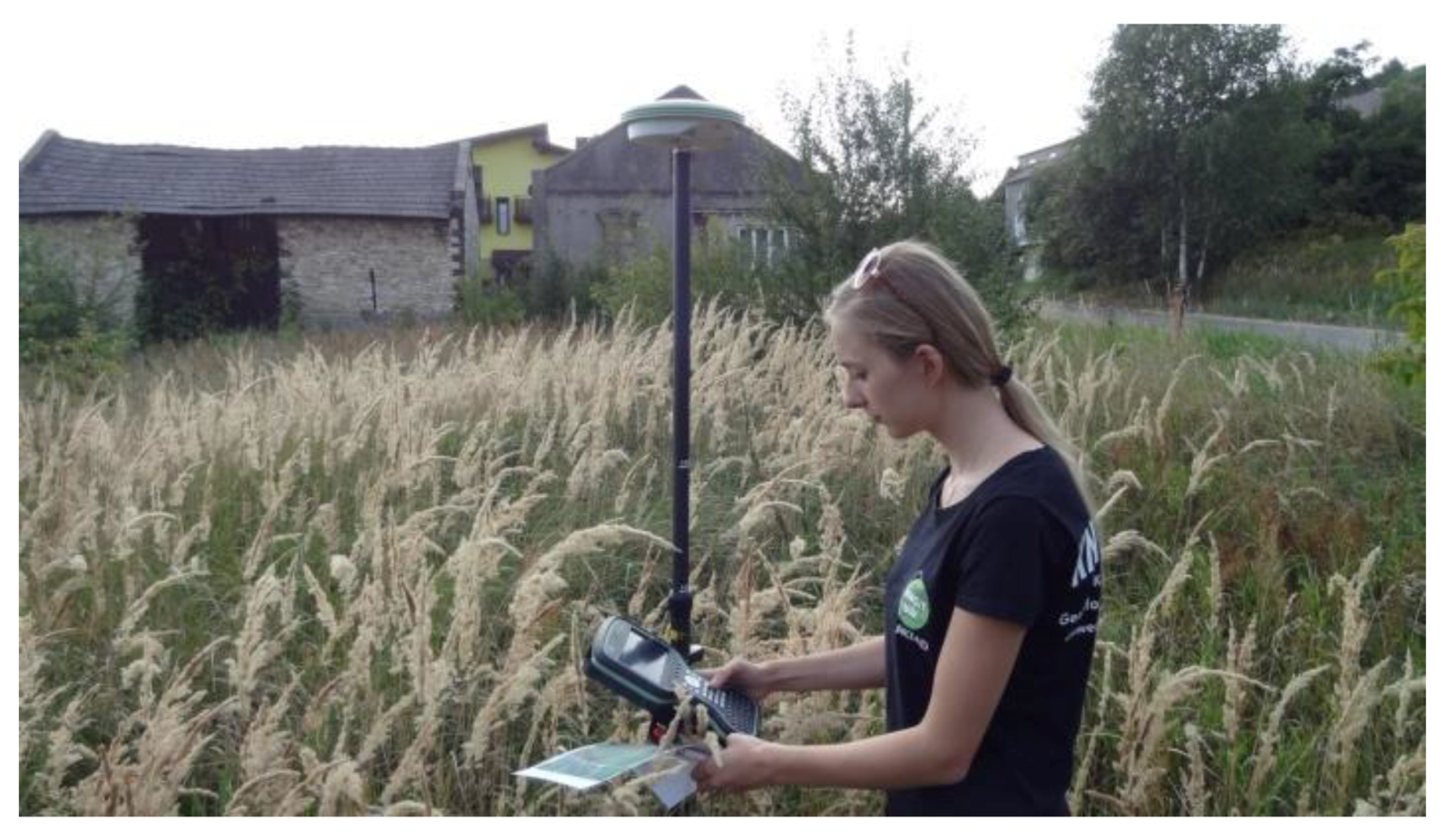
2.2. Field Measurements

The field studies were conducted in the summer of 2017. Compact polygons (in the shape of circles with a radius of 3 meters) of Rubus spp., Solidago spp., Calamagrostis epigejos, and other background plants were located within the research area with the help of the Leica CS20 GNSS device (Figure 2). The number of polygons was proportional to the prevalence of species in the research area and amounted to 50 polygons for blackberry and wood small-reed, 60 polygons for goldenrod, and 100 polygons for background plants.
Then, the polygons were transferred to ArcMap 10.3, where photo interpretation techniques were used to create an additional 30 reference polygons for other types of land cover (i.e., trees, buildings, bare soil, and shaded areas). These additional classes were meant to indicate for the algorithm the spectral properties of objects that occurred in the research area and constituted non-forest vegetation. Finally, reference polygons were created for eight classes: Calamagrostis epigejos, Solidago spp., Rubus spp., other plants, trees, bare soils, buildings, and shadows (Figure 1).

2.3. Airborne Hyperspectral HySpex Data

Aerial hyperspectral data were obtained by MGGP Aero Sp. z o.o. on 29 August 2017 using sensors located on a Cessna 402B aircraft. A hyperspectral image with a 16-bit radiometric resolution was recorded with two HySpex Visible and Near Infrared (VNIR-1800) scanners and a Shortwave Infrared (SWIR-384) scanner. The specification of both sensors is provided in the table below (Table 1).
The aerial hyperspectral images were prepared for further processing in accordance with the diagram presented in the schema (Figure 3). The data obtained by hyperspectral sensors were converted to radiance units with HySpex RAD software. Then, the hyperspectral image was subjected to geometric correction, which employed the digital surface model in PARGE (PARametric GEocoding) software (ReSe Applications LLC, Wil, Switzerland), and atmospheric correction was performed with the MODTRAN5 model in ATCOR4 (ATmospheric CORrection) software (ReSe Applications LLC, Wil, Switzerland). Nine flight lines were mosaicked and re-sampled to achieve a uniform spatial resolution of 1 m. Next, the last 21 bands in the SWIR range were removed because of the high level of noise caused by the sensor’s lower SNR (Signal to Noise Ratio) at the extreme ranges of the imaged spectrum, which ultimately resulted in a 430-band image in the spectral range of 416.18–2396.44 nm.
In order to reduce HySpex data dimensionality, Minimum Noise Fraction (MNF) transformation was applied. Based on MNF bands, eigenvalues, and visual assessment of transformed bands, the first 30 MNF bands were selected for further processing. Finally, two data sets were prepared for species classification: the first one contained 430 HySpex bands while the second one contained 30 MNF bands.

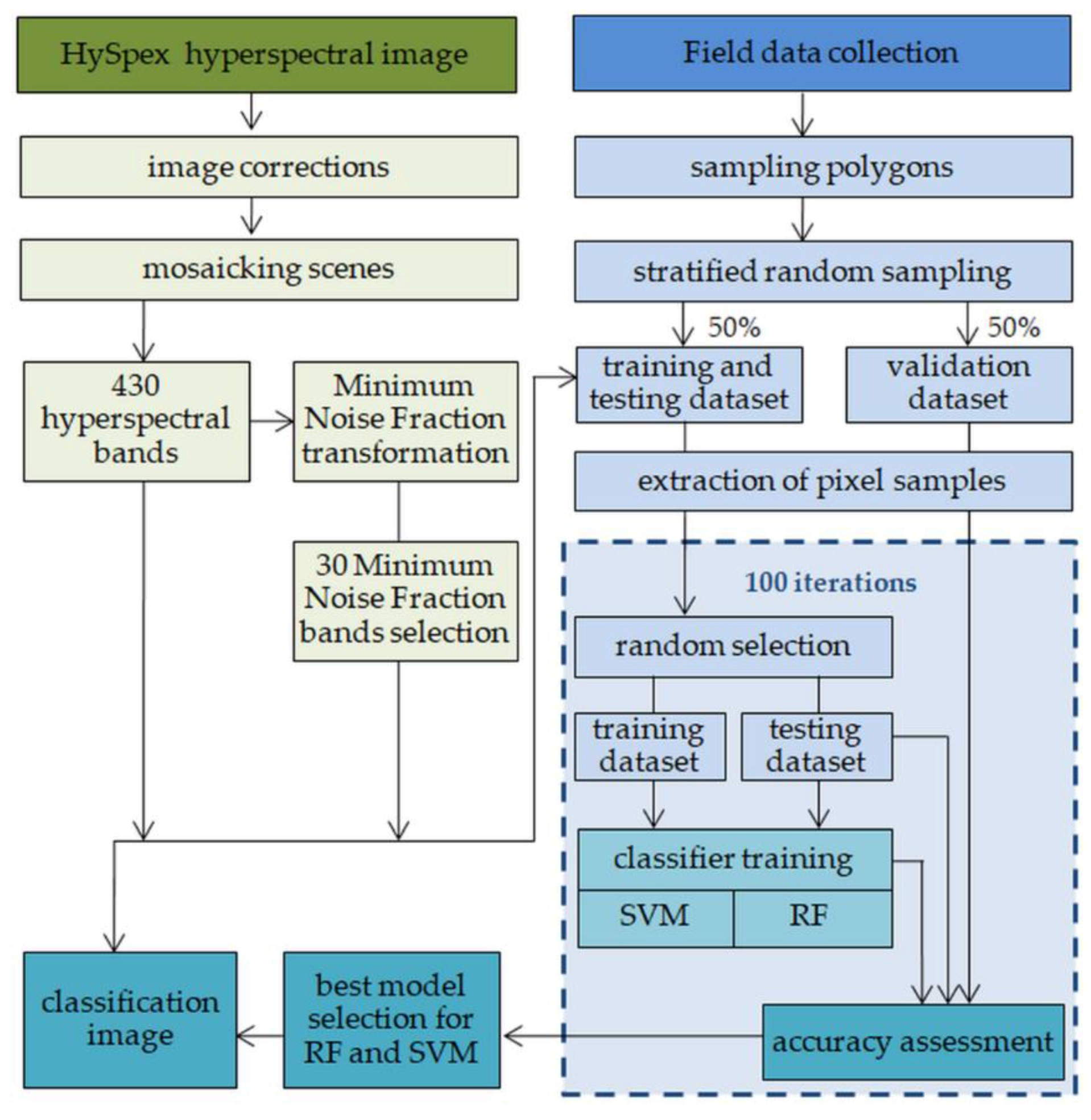
2.4. Classification Process and Accuracy Assessment

One of our goals was to analyze the impact of pixel number in the training data sets on classification accuracy; hence, we created training data sets with a set number of pixels per class. Using stratified random sampling, 50% of all reference polygons were selected to create a training test data set, while remaining polygons were used to create a validation data set.
The training test data set was used to create subsets (training data sets with a set number of pixels per class), and all remaining samples ended up in the test data set that was used for preliminary accuracy assessment. The validation data set was created to eliminate spatial autocorrelation with the training test data set (randomly selected pixels were used in the training and validation sets). This allowed to create a spatially independent and stable validation data set, which was used to assess final results.
To investigate the influence of training data set size on achieved classification results, the training test data set was sub-sampled to create training data sets that contained exactly 30, 50, 100, 200, and 300 pixels per class. These sub-sampled data sets will be used for classifier training. If a given class had fewer total available samples than required, random sampling with replacement was used, otherwise random sampling without replacement was employed. If all available pixels for given class were selected for training purposes, a copy of training data for this class was used instead.
An iterative accuracy assessment was used in order to objectively compare achieved results. This was a procedure consisting of the following steps repeated 100 times:
  • Sub-sample the training test data set in order to create a training data set with a set number of samples per class;
  • Train SVM and RF classifiers;
  • Assess accuracy using test and validation data sets; and
  • Save trained classifier models and accuracy measures for further analysis.
Pixel classification was carried out on the basis of the Support Vector Machine and Random Forest algorithms in R software. The first stage of the training process was to optimize the learning parameters of these algorithms in order to obtain the best possible settings. This task was completed on the training and test sets before the division. A radial basis function was chosen for the SVM algorithm because of its proven efficiency [43] and smaller number of computational difficulties [44]. The learning parameters of the compared classification algorithms were subjected to a tuning process. A gamma value of 0.1 and cost of 1000 was obtained for the SVM algorithm. In the case of the Random Forest algorithm, on the basis of the out-of-bag (OOB) error analysis, the mtry parameter (the number of features randomly sampled at each split) was set at 140 for classification on 430 hyperspectral bands and at 13 for classification on the set of the first 30 MNF transformation bands. In both cases, the number of random trees (ntree) amounted to 500.
In this work, we compared two classification algorithms (SVM and RF), two different data sets (430 original hyperspectral bands, 430 HS, and 30 Minimum Noise Fraction bands, 30 MNF), and five different sample sizes per class in the training data set (30, 50, 100, 200, and 300 pixels). Due to the unavailability of the larger continuous areas of invasive plants on our study area, we have limited the analysis to 300 pixels. All combinations of the above parameters were tested, resulting in 20 different classification scenarios.
Accuracy of the performed classifier training was assessed with the set of test data and the data spatially separated from the training and test set (i.e., on pixels of the validation data set), which was constant for all scenarios. The algorithms were compared, and the best combination of image data set and classifier was determined based on validation performance. The following accuracy parameters were calculated on the basis of the error matrix:
  • Overall accuracy—the ratio of the total number of correctly classified pixels to the total number of reference pixels [45];
  • Cohen’s Kappa—the similarity of the analyzed classification compared to the random classification (a Kappa value of 0 means full similarity while 1 means no similarity) [46];
  • Producer’s Accuracy (PA)—the ratio of correctly classified pixels of a given class to all pixels in the validation data set for this class [45];
  • User’s Accuracy (UA)—the ratio of pixels correctly classified in a given class to all pixels classified in this category [45]; and
  • F1 score sensitivity, measured using harmonic mean of precision (P), positive predictive value, and recall (R) as in Equation (1) [47,48]:
F = 2PR/(P+R)
Afterwards, the best models for each classifier and data set were selected on the basis of the mean F1 scores for all classes (based on the validation data), and the images were classified. The significance of statistical differences between the accuracy of the models was checked using the Mann–Whitney–Wilcoxon test [49] (significance level = 0.05). The Mann–Whitney–Wilcoxon test is well suited for testing differences between non-normally distributed populations [26,50]. Distributions of achieved accuracy measures for all classification scenarios were visualized using box plots. A detailed explanation of boxes used in box plots is shown in Figure 4.
Moreover, classifier training was performed on nine classes, each with an identical number of training samples to reduce any effect of unbalanced training data. After classifier training, background classes were considered as one class with relation to plant classes. Such steps allowed us to properly assess classification quality (which classes are confused with which) and helped us achieve the most accurate results. In our work we assumed that confusion between background classes was acceptable, while confusion between plant species and background classes or other plant species would be a concern that would need to be addressed and reported. When classifying plant species, it is important to deliver a suitable and representative sample of pixels that characterize objects other than object of the study. Such classes can be oftentimes referred to as background classes. Since our study aimed to investigate the influence of training data set size, it would be insufficient to perform classification of four classes, that is, three plant species and one class with background objects. This mainly is due to difficulties in randomly sampling background classes in such a way that, for example, 30 pixels will represent them all. In fact, such an approach would almost guarantee that pixels for background classes covering a relatively small area would not be included in the training data set with a sufficient number of samples, which in turn would destroy any credibility of such work. To address this issue when creating the training data set, each background class (shadows, trees, other plants, soils, and buildings) had the same number of training samples, equal to the number of samples used for each plant species class. This is to ensure our background classes had similar representation to the plant species classes during classifier training.

3. Results

3.1. Statistical Analysis of Investigated Classification Scenarios

The mean F1 score was calculated for all classes on two sets: the test set and the validation set. The test set was dependent on the training set—the pixels in these sets were drawn from the same polygons, so the number of pixels in the test set decreased with an increasing number of pixels in the training set (Table 2). The high accuracy level obtained for this set is, therefore, not surprising, nor can it be used to compare the classifiers.
In contrast, the validation set had a fixed number of observations (4835 pixels) and was spatially independent of the other data sets. Regardless of the classifier used, higher mean F1 scores for all classes based on the validation set were obtained for classifications performed on 30 MNF transformation bands (0.854–0.918) compared to that of the 430 hyperspectral data bands (0.760–0.853).
The accuracy level for both classifiers increased with the number of training pixels used for classification (Figure 5). The distributions of the mean F1 score for all classes revealed that when the number of training pixels increased, the interquartile range of the obtained accuracies decreased, so the results obtained in 100 iterations were more stable. What is more, the use of a smaller number of training pixels caused a greater decrease in the accuracy of classifications performed on the original hyperspectral bands than in the case of classifications performed on the MNF transformation bands. The most stable distributions and the highest F1 scores for all classes were obtained by the classifications performed on a set of 30 MNF transformation bands and 300 training pixels (the median F1 for RF was about 0.92, while the median F1 for SVM was about 0.88).
In order to check if there are statistically significant differences in the F1 scores of all the tested scenarios, the Mann–Whitney–Wilcoxon test was carried out at the significance level of 0.05 (Figure 6). There were statistically significant differences between most of the considered scenarios. The SVM classifications on MNF bands using 200 and 300 pixels for classifier training were the only exception. There were no statistically significant differences found for the RF classification performed on 430 hyperspectral bands using 300 training pixels and the SVM classification on a very limited data set consisting of 30 MNF bands and 30 training pixels.
An analysis of the distribution of F1 scores for individual classes of identified species (Figure 7) makes it possible to draw conclusions about the best data sets and algorithms for classifying each class.
The Solidago spp. class identified well with all classifiers and raster data sets (the F1 score was above 0.95). The accuracy levels increased with an increasing number of training pixels, whereas the differences in accuracy levels resulting from the change in the size of the training sets were small. However, slightly higher mean F1 scores were recorded for the Random Forest classifier. Solidago are marked by their very characteristic yellow color and spectral properties, which distinguished them from other classes in the imaging, and additionally tend to form large, uniform fields, so the almost perfect identification of this species was not surprising.
In the case of the Rubus spp. class, the best identification results were obtained for the SVM classification on 30 MNF bands using 300 training pixels (F1 = 0.97), but application of the same classifier with the number of training pixels reduced to 100 resulted in a similar accuracy level. Good results were also obtained for the RF classification on the same raster data set and 300 training pixels (F1 = 0.95). The F1 scores obtained on 430 hyperspectral data bands were lower (F1 RF from 0.7 to 0.76, and F1 SVM from 0.71 to 0.84).
Calamagrostis epigejos was a more difficult plant species to identify. However, high F1 scores of around 0.91 were obtained using the SVM algorithm, 30 MNF transformation bands, and sets of 200 and 300 training pixels. A similar accuracy level was also obtained for the SVM classification and 300 training pixels on 430 hyperspectral bands (F1 = 0.9). The Random Forest classification resulted in lower accuracy levels for this species, with F1 scores between 0.7 and 0.82 on the hyperspectral data set, and between 0.76 and 0.83 on the MNF transformation bands. The accuracy increased with the growth of the number of training pixels.
Considering the mean accuracy level for three species identified in the research area, it can be concluded that the best spatial distribution was obtained using the SVM algorithm and 200 or 300 training pixels (F1 = 0.95). For the other classes distinguished in the image (i.e., plant background, forests, buildings, bare soil, and shadows), the best F1 scores (from 0.93 to 0.96) were obtained with the RF algorithm. However, in terms of accuracy for all the classes together, the best accuracy (Kappa = 0.92, F1 for all classes = 0.92) was obtained for the RF classifier, 30 MNF bands, and sets of 200 and 300 training pixels.
To sum up, the SVM algorithm and the data set consisting of 30 MNF bands and 300 training pixels proved to be the best for identifying the Calamagrostis and Rubus classes. In the case of Solidago and background classes, better results were obtained with the Random Forest classifier. However, goldenrod classified well (mean F1> 0.95) on both sets of raster data and with a different numbers of training pixels. On the other hand, in the case of background classes, the best results were obtained for 30 MNF bands and 200 training pixels. This may indicate that the Random Forest method works better for the classification of spectrally uniform, large forms of land use, which differ significantly from their surroundings, while the SVM method is better for identifying plant species that are more spectrally different and similar to the background classes.

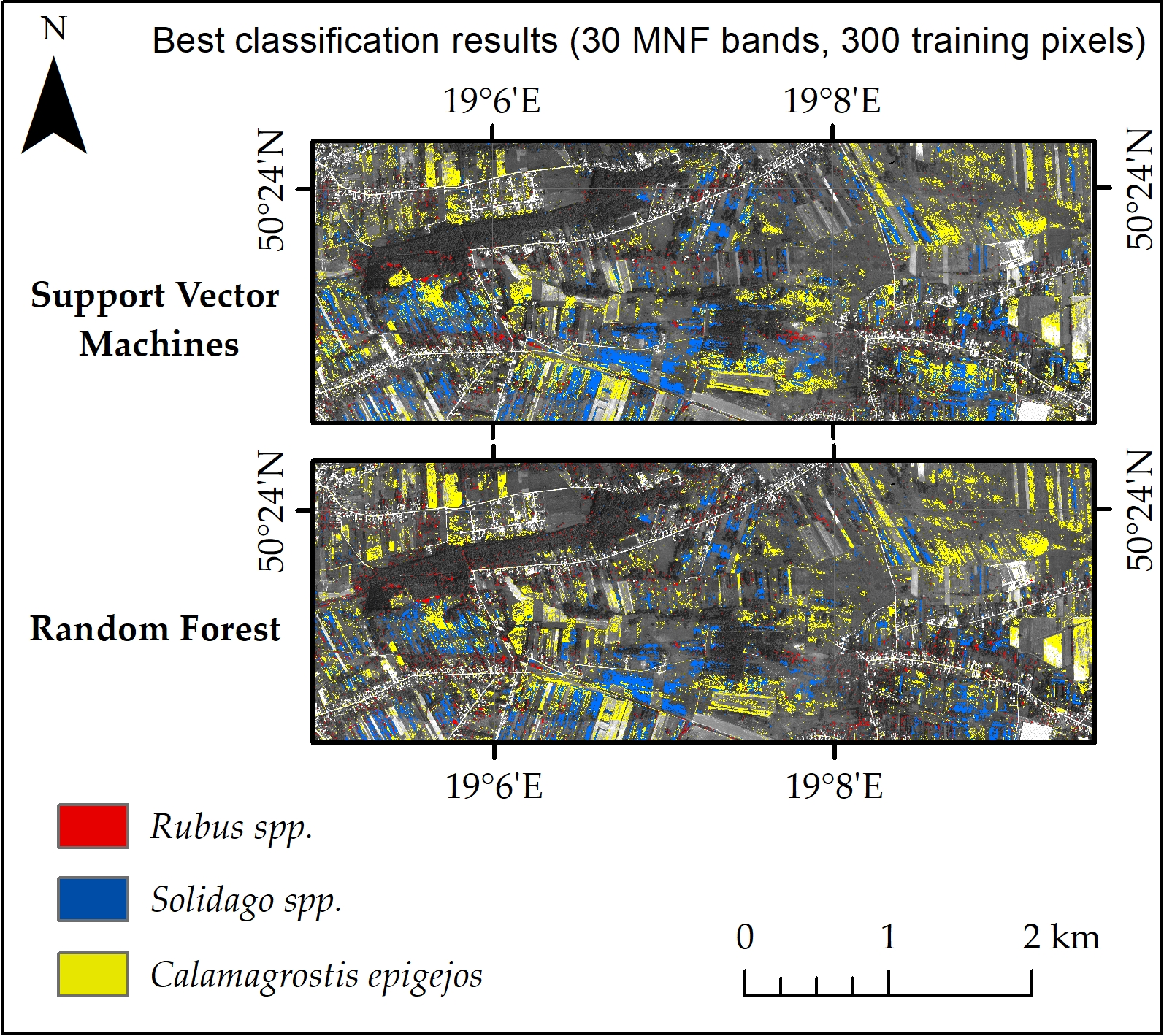
3.2. Best Model Plant Species Identification Accuracy

A set of data consisting of 30 MNF bands and 300 training pixels was selected on the basis of the analysis of statistical accuracy to develop images showing spatial distributions of the analyzed species in the research area. Figure 8 presents distributions of the producer and user accuracies for 100 iterations of classifications performed on a selected set of data using both classifiers.
For the Rubus spp. class, the RF classifier yielded a lower median user’s accuracy than that of SVM by three percentage points, while the differences in the producer’s accuracy levels between the classifiers were small. Both the producer’s and user’s accuracies for Solidago spp. were very high (close to 100%), a slight underestimation was detected only in the case of the SVM classification (producer’s accuracy about 93%). In contrast, the Calamagrostis epigejos class achieved the lowest median producer and user accuracies of all classes. The SVM classifier achieved higher producer and user accuracy levels for C. epigejos (PA = 96%, UA = 87%) than the RF classifier (PA = 88%, UA = 78%).
The resulting images for both classification methods prepared for the best mean F1 scores for all iteration classes are presented and compared below (Figure 9). The correctness of species identification was also assessed on the basis of the confusion matrix (Table 3 and Table 4).
Rubus spp. was identified near forest borders and buildings, and its spatial distribution for the SVM method reflected reality more accurately than the result of using the RF method (Figure 9). There was a slight overestimation of this species in the case of the RF method, especially in places with trees and bushes near buildings (Table 4). The Calamagrostis epigejos and Solidago spp. classes can be found in the open spaces of non-agricultural meadows. The spatial distribution of Solidago in the image resulting from the use of the RF method reflected reality almost perfectly, and in the case of the SVM method, the underestimation of this species applied mainly to uncut meadows in the south of the area. On the other hand, the Calamagrostis epigejos class was slightly overestimated in the results of both classifications, especially in places with dry or mowed meadows. The SVM classification image presents the spatial distribution of this species in the research area with greater precision (Table 3), and its estimations were more accurate, especially in places with bare soils, which have a similar spectral response.

4. Discussion

The effects of the raster data set and the number of training pixels on the classification accuracy of three invasive or expansive plant species were tested in this paper using the Random Forest and Support Vector Machine methods. The method we used to divide the patterns into three sets—the training set, the test set, and the spatially independent validation set—allows for reliable assessment of the classification accuracy. Balanced training sets of 30, 50, 100, 200, and 300 pixels per class were tested in this paper. The test set was strongly spatially correlated with the training set, which led to inflated accuracy results; therefore, it was used only for the initial accuracy assessment. However, surprisingly accurate measures (PA, UA, F1) calculated on the test data set increased, despite the decrease in the number of patterns in the test set. This highlights the importance of using spatially separate data set for proper accuracy assessments. A constant set of validation pixels that remained both unchanged between iterations and was spatially separate from training data allowed us to reliably assess the accuracy of classification. Spatial separation of the data sets used to assess classification results and train classifiers allowed us to avoid artificial inflation due to spatial correlation between pixels belonging to the same reference polygon. Such a method allows for more objective comparisons of classification algorithms and data sets, while delivering more trustworthy accuracy metrics. The very act of creating training and test or validation data sets introduces human or random bias into any comparison. In order to decrease such bias of our method, training and validation data sets were created multiple times. Such approaches were already used multiple times in the past [24,51,52] and are proven to be more reliable when it comes to classifier comparison. The accuracy of any machine learning procedure is directly related to the quality of samples used for training and validation of a given classifier. In order to decrease the impact of human or random bias in creating the data sets, training and validation data sets were created multiple times. Repeated sampling of pixels for the reference sets and assessing classification accuracy minimized the impact of pixel selection for training on the classification accuracy and allowed an objective assessment of the impact of the tested data sets on the effectiveness of species identification [26,52,53].
The analyses showed that, regardless of the selected classifier, a higher F1 score for all classes was obtained for classifications performed on 30 MNF transformation bands (0.854–0.918) than those on 430 hyperspectral data bands (0.760–0.853). The reduction in the number of input layers to several dozen of the most informative bands is recommended for the Random Forest and Support Vector Machine algorithms, as it allows one to obtain higher accuracy levels and significantly shortens the classification time [51,54,55,56]. During the classification of herbaceous vegetation in the Hortobágy National Park (Eastern Hungary), a higher overall accuracy level was obtained for nine MNF transformation bands (SVM = 82.06%, RF = 79.14%) than for 128 original bands of AISA Eagle (SVM = 72.85%, RF = 72.89%) [27]. Similarly, when identifying tree species based on AISA Eagle data using the SVM algorithm, classification of the MNF-transformed data resulted in an increase of about 30% in the classification agreement compared to the classification performed on the original bands [57]. The first 30 MNF transformation bands were used, for example, to identify four invasive or expansive species in central Poland, obtaining high F1 scores of identification: about 0.80 for Filipendula ulmaria and Molinia caerulea, about 0.79 for Phragmites australis, and about 0.73 for Solidago gigantean [58].
The increase in the number of pixels used to train the F1 score classification for the three species analyzed in this article resulted in an increase of these values, but also a simultaneous decrease in their distribution width, which indicates stabilization of the results. Our observations indicate that the preferred number of training patterns is at least 300 pixels per class, regardless of the classifier used. In the case of 30 MNF and the SVM algorithm, 300 was the optimal value because there were no statistically significant differences between training data sets containing 200 and 300 pixels per class (Figure 6). Due to the unavailability of the larger continuous areas of invasive plants on our research area, we have limited the analysis to 300 pixels, and therefore we were unable to assess impact of larger number of pixels per class in training data set on achieved classification results. A similar trend was noticed by testing different sets of training pixels (from 10 to 30 pixels) and raster data for the classification of 20 herbaceous species in Eastern Hungary by means of the SVM and RF algorithms [27]. Moreover, the highest overall accuracy (SVM: 82.06%; RF: 79.14%) was obtained using the largest of the tested sets of patterns (30 training pixels). The overall classification accuracy decreased with a decreasing number of training pixels (lower by about 2 percentage points for the set of 10 training pixels).
After a detailed analysis, it can be concluded that the Support Vector Machine algorithm was more resistant to smaller numbers of training patterns and allowed to obtain a higher mean F1 score for three plant species (F1 SVM = 0.95) compared to the Random Forest algorithm (F1 RF = 0.92) on the best data set (30 MNF, 300 training pixels). Lower mean F1 scores for background classes (F1 SVM = 0.82, F1 RF = 0.91) were noted in the SVM result image, but classification errors occurred mainly between different background classes and not between the background and plant species.
Visual interpretation of the result images and statistical accuracy analyses indicated that both classifiers detected the plant species of this study in the research area with a very high level of accuracy. Correct identification of species was also confirmed by additional field verifications carried out after the analyses. High classification accuracy levels obtained for the analyzed scenarios may also be due to the optimal time in which the imaging was obtained [26,59]. The analyzed species are in their flowering and fruiting phases at the turn of August and September, which makes them more distinctive thanks to their characteristic colors of inflorescences, fruits, and leaves (Table 5).
The classification accuracy of the Solidago spp. species was very high (F1> 0.95) for both classifiers and the raster data. This is not surprising because this plant’s yellow inflorescences form homogeneous fields, which are easy to distinguish from other objects in images, and it would probably be even possible to use photointerpretation for this task. The Solidago gigantea species was identified in central Poland using 30 MNF transformation bands (a mosaic of hyperspectral data from the same HySpex sensors) and the Random Forest method; a lower F1 score for the species, about 0.73, and a slightly higher F1 score for the background, about 0.94, were obtained [58]. Solidago spp. has also been classified with high accuracy (F1 about 0.83, UA = 0.71, PA = 1.0) on the Hungarian–Slovak cross-border site using 15 MNF bands (a mosaic of hyperspectral data from AISA Eagle II) and the maximum likelihood method [61]. High identification accuracy of one of the goldenrod species, Solidago altissima (F1 score of about 0.86, UA = 0.94, PA = 0.80), was also obtained during the research conducted in Watarase wetlands in Japan with the help of only 3 MNF transformation bands (a mosaic of hyperspectral data from AISA Eagle) and generalized linear models [19].
Rubus spp. was classified in the research area with F1 scores ranging from 0.70 to 0.97, with the highest accuracy obtained for the Support Vector Machine method and 30 MNF transformation bands. High accuracy (OA = 87.8% and Kappa = 0.75) was also obtained during the detection of Rubus armeniacus in open areas in Surrey, BC, Canada, by means of a combination of CASI hyperspectral imagery with LiDAR data and the Random Forest algorithm [62]. Similarly, when identifying Rubus fruticosus sp. agg. in the Kosciuszko National Park in Australia, a F1 score of about 0.83 was obtained for blackberry using 23 bands of a mosaic of hyperspectral data from HyMap after MNF transformation and the Mixture-Tuned Matched Filter (MTMF) algorithm [32]. On the other hand, research on the identification of Rubus cuneifolius species in the eastern parts of South Africa using the SVM algorithm and multispectral data led to results that were much lower in accuracy: the F1 scores for the Landsat data varied from 0.33 to 0.48, while the scores for the Sentinel-2 data were between 0.34 and 0.58, which confirms that hyperspectral data allow for much more accurate detection of blackberries [63].
Identification of Calamagrostis epigejos resulted in F1 scores between 0.70 and 0.91, depending on the algorithm and data set used. As before, the best data set for wood small-reed classification turned out to be the SVM algorithm and MNF-transformed bands (F1 scores from 0.86 to 0.91), while the RF method resulted in F1 scores between 0.76 and 0.83, depending on the number of pixels used for training. By carrying out C. epigejos classifications at various growth stages, it was confirmed that flowering time (around September) facilitated correct identification of wood small-reed [26]. In addition, the use of the Random Forest method and MNF transformation bands on the HySpex hyperspectral data led to an F1 score of 0.72, which is an accuracy level close to the one obtained for wood small-reed in our research. Lower accuracy was obtained (producer accuracy 68%, and user accuracy 51%) in the classification of plant communities representing the Calamagrostis villosa species when the APEX data and the SVM method were used [60]. However, an average PA of about 82% and UA of about 75% were obtained for wood small-reed grasses during the classification of high-mountain vegetation communities using 40 MNF transformation bands of the DAIS 7915 data and neural networks [64]. This was similar to the results obtained in our work on 30 MNF bands with the RF algorithm (PA of about 88%, UA of about 78%) and was lower than the results for SVM (PA of about 96%, UA of about 87%).

5. Conclusions

The above-presented research concerning identification of three species of invasive or expansive plants using the Random Forest and Support Vector Machine classification methods, as well as various sets of input data, has led to the following conclusions:
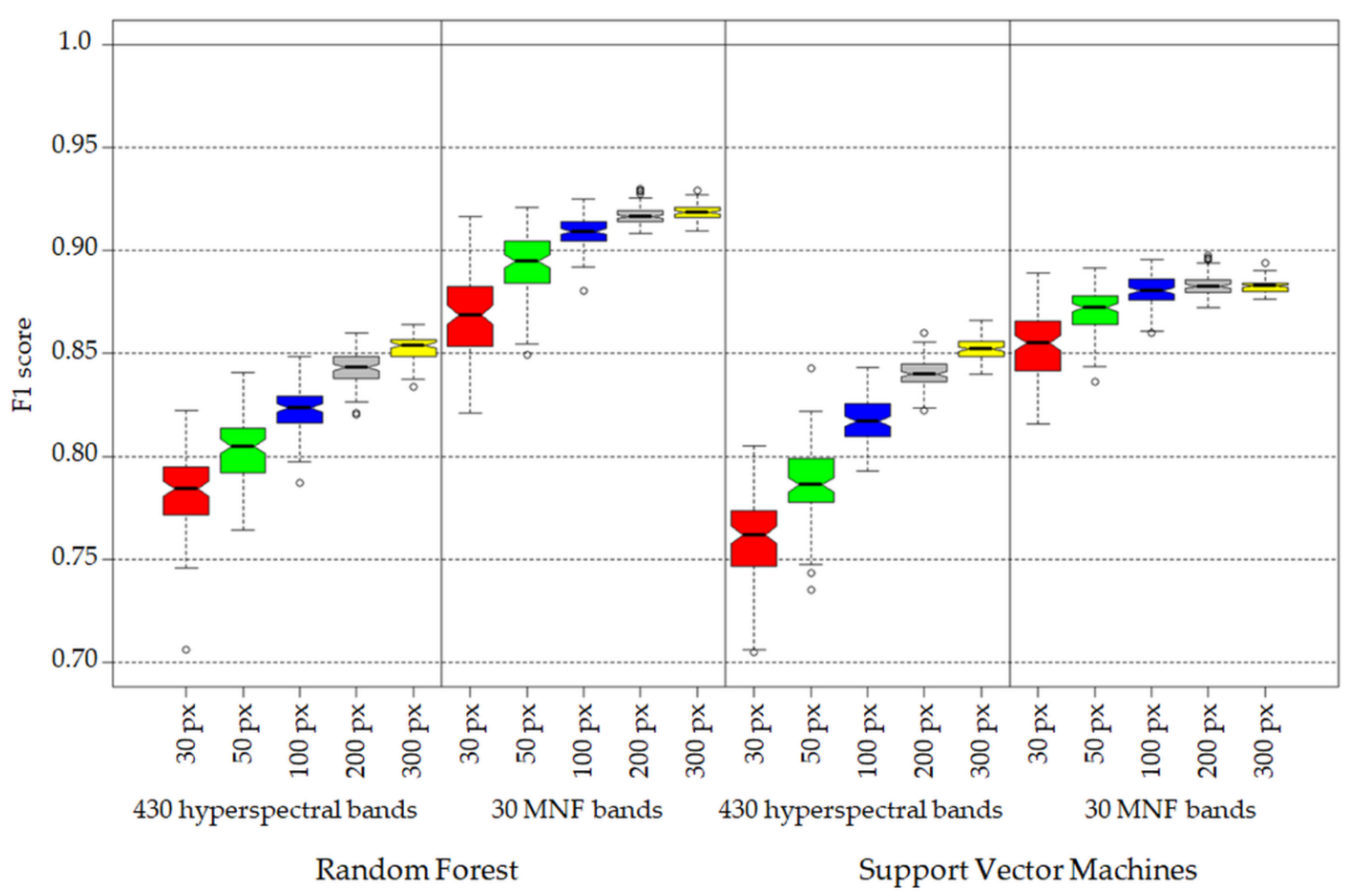
  • The accuracy assessment method presented in the paper allows us to confirm that all analyzed species can be identified in heterogenous habitats (achieved classification results F1 oscillated around 0.90). The species created a unique set of spectral properties, which are recognizable by the SVM and RF classifiers, and separating training and validation sets at the level of the reference polygons, and not at the level of individual pixels, is justified. This allows one to avoid overestimating the accuracy of the results due to spatial correlation of pixels from the same reference polygon. We have shown a clear need to divide classes into training and validation at the polygon level in order to minimize spatial correlation between samples and in order to achieve unbiased and accurate classification metrics. A spatially separate and unchanging validation set can be used to improve the quality of the obtained accuracy scores and compare the results more objectively. Unfortunately, this type of approach makes it more difficult to use iterative methods of assessing accuracy or significantly reduces the number of observations in a data set that can be used for classifier training. What is more, the principles of a constant and unchanging validation set are not optimal, which may negatively affect the quality of the resulting post-classification images. A set of 30 MNF bands allows for more accurate identification of the analyzed invasive and expansive plant species than that of the 430 original spectral bands of the HySpex image.
  • Increase of number of pixels per class in training data set has a greater effect on achieved accuracy measures in the case of 430 spectral bands data set (difference in medians between 30 and 300 pixel data sets around 8 percentage points (p.p.) in the case of RF and 9 p.p. in the case of SVM algorithm) then in the case of 30 MNF bands data set (median difference between 30 and 300 pixel data set: 5 p. p. for RF and 3 p.p for SVM, Figure 7).
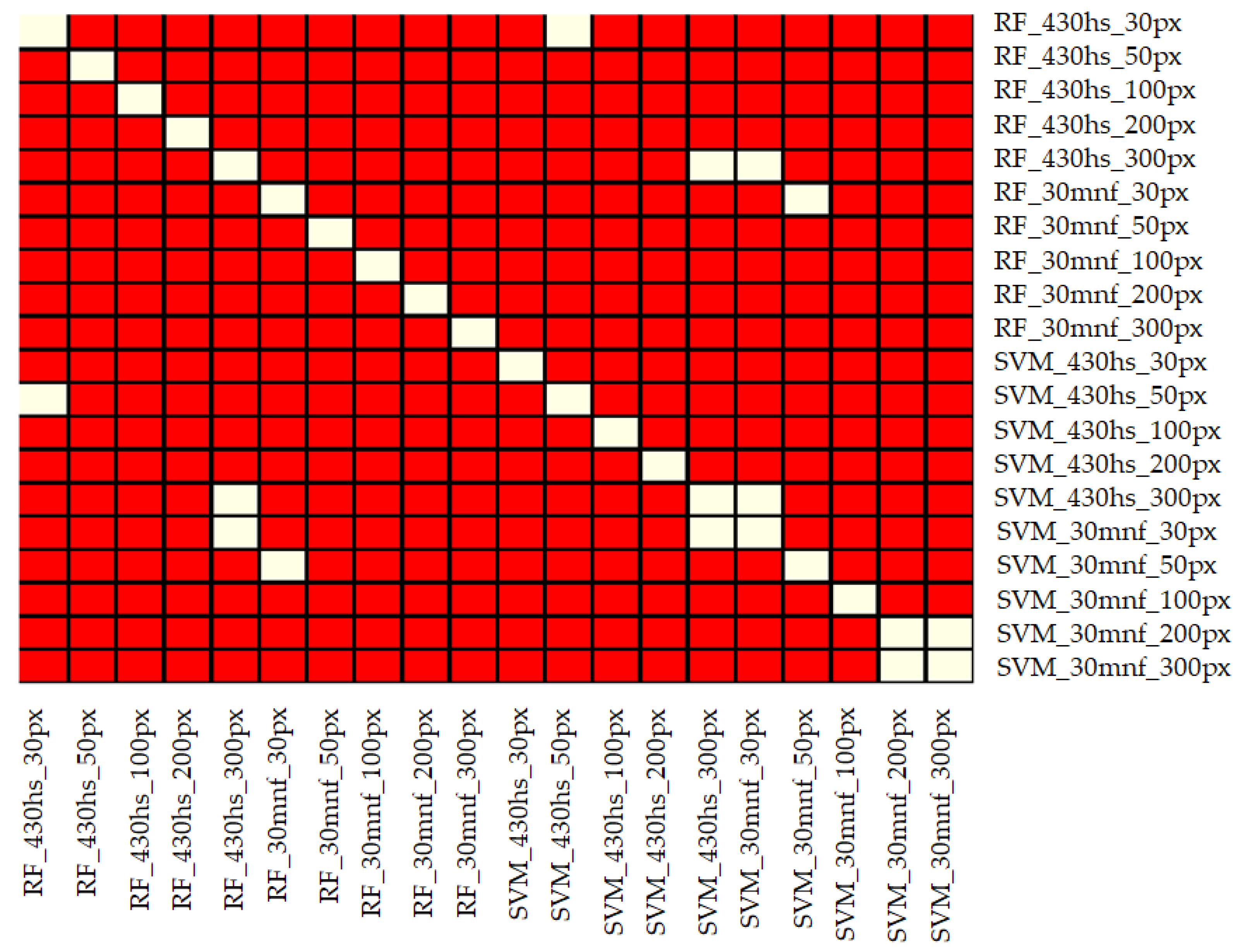
  • Three hundred pixels per class is the preferred number of samples in the training set for classification of the analyzed plant species with the help of the SVM and RF methods. Fewer pixels result in a significant decrease in classification accuracy and less stable results. In our case, we managed to find the optimal number of pixels in training data sets per class only in the case of the SVM classifier applied to MNF data. Figure 6 shows that there was no significant statistical difference between tests performed on MNF bands with 200 and 300 pixel samples per class. Hence, 200 pixels per class in the training data set for 30 MNF bands and the SVM classifier is optimal.
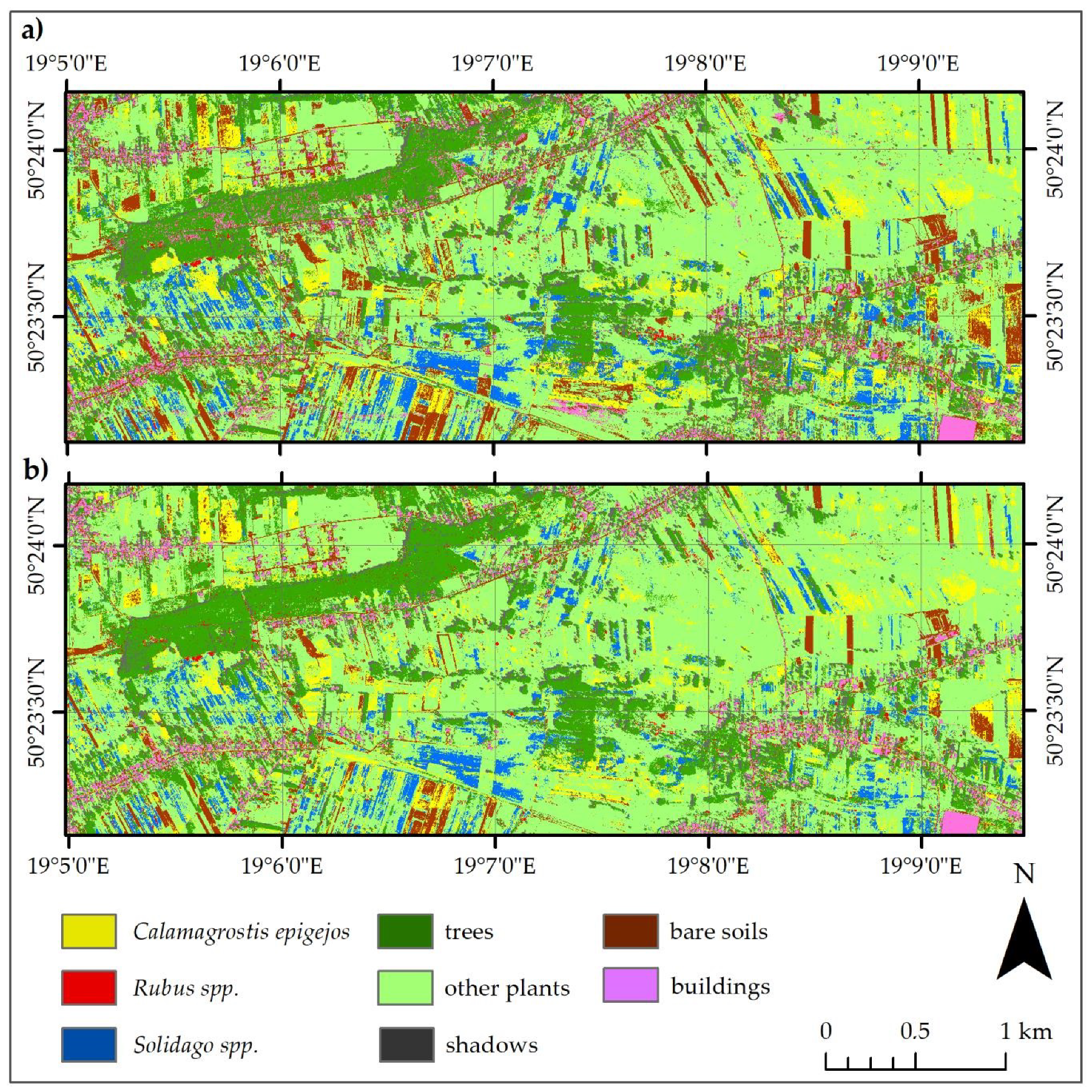
  • Both the Support Vector Machine method and the Random Forest method allowed us to obtain very accurate images of the distribution of analyzed species in the research area. However, the SVM classifier worked better for the classification of blackberry and wood small-reed (i.e., for classes that are not uniform and do not differ spectrally from their surroundings). On the other hand, the Random Forest algorithm allows one to obtain a higher accuracy for homogeneous classes that stand out spectrally (i.e., goldenrod and background classes). Still, the SVM image was found to be more reliable, despite its relatively lower accuracy for the background classes. Most classification errors occurred between background classes rather than individual species.

Author Contributions

Conceptualization, A.S.-T. and B.Z.; methodology, A.S.-T. and E.R.; software, E.R.; validation, E.R. and A.S.-T.; formal analysis, A.S.-T. and E.R.; investigation, A.S.-T. and E.R.; data curation, A.S.-T.; writing—original draft preparation, A.S.-T.; writing—review and editing, B.Z. and E.R.; visualization, A.S.-T. and E.R.; supervision, B.Z. All authors have read and agreed to the published version of the manuscript.

Funding

This research has been carried out under the Biostrateg Programme of the Polish National Centre for Research and Development (NCBiR), “Natural Environment, Agriculture and Forestry” project DZP/BIOSTRATEG-II/390/2015: The innovative approach supporting monitoring of non-forest Natura 2000 habitats, using remote sensing methods (HabitARS, Consortium Leader: MGGP Aero; the project partners include the University of Lodz, the University of Warsaw, Warsaw University of Life Sciences, the Institute of Technology and Life Sciences, the University of Silesia in Katowice, Warsaw University of Technology). The publishing costs were covered by the Polish Ministry of Science and Higher Education, project the theme No. 500-D119-12-1190000.

Acknowledgments

The authors would like to thank the HabitARS Consortium, especially MGGP Aero for acquiring, pre-processing, and sharing the HySpex data. Data fusion procedures were conducted in the frame of the H2020-MSCA-RISE-2016: innoVation in geOspatiaL and 3D daTA (VOLTA), Reference GA No. 734687. H2020 VOLTA activities are supported by the Polish Ministry of Science and Higher Education in the frame of H2020 co-financed projects No. 3934/H2020/2018/2 and 379067/PnH/2017. We are also grateful to the editors and anonymous reviewers for their constructive comments and suggestions that helped to improve this manuscript.

Conflicts of Interest

The authors declare no conflicts of interest.

References

  1. Mooney, H.A.; Cleland, E.E. The evolutionary impact of invasive species. Proc. Natl. Acad. Sci. USA 2001, 98, 5446–5451. [Google Scholar] [CrossRef] [PubMed] [Green Version]
  2. Tokarska-Guzik, B.; Dajdok, Z.; Zając, M.; Zając, A.; Urbisz, A.; Danielewicz, W.; Hołdyński, C. Rośliny Obcego Pochodzenia w Polsce ze Szczególnym Uwzględnieniem Gatunków Inwazyjnych; Generalna Dyrekcja Ochrony Środowiska: Warszawa, Poland, 2012; ISBN 978-83-62940-34-9. [Google Scholar]
  3. Hulme, P.E.; Pyšek, P.; Nentwig, W.; Vilà, M. Will Threat of Biological Invasions Unite the European Union? Science 2009, 324, 40–41. [Google Scholar] [CrossRef] [PubMed] [Green Version]
  4. Holub, P.; Tůma, I.; Fiala, K. The effect of nitrogen addition on biomass production and competition in three expansive tall grasses. Environ. Pollut. 2012, 170, 211–216. [Google Scholar] [CrossRef] [PubMed]
  5. Pruchniewicz, D.; Żołnierz, L. The influence of environmental factors and management methods on the vegetation of mesic grasslands in a central European mountain range. Flora-Morphol. Distrib. Funct. Ecol. Plants 2014, 209, 687–692. [Google Scholar] [CrossRef]
  6. Babai, D.; Molnár, Z. Small-scale traditional management of highly species-rich grasslands in the Carpathians. Agric. Ecosyst. Environ. 2014, 182, 123–130. [Google Scholar] [CrossRef]
  7. Sedláková, I.; Fiala, K. Ecological problems of degradation of alluvial meadows due to expanding Calamagrostis epigejos. Ekol. Bratisl. 2001, 20, 226–233. [Google Scholar]
  8. Huang, C.-Y.; Asner, G. Applications of Remote Sensing to Alien Invasive Plant Studies. Sensors 2009, 9, 4869–4889. [Google Scholar] [CrossRef] [Green Version]
  9. Sabat-Tomala, A.; Jarocińska, A.M.; Zagajewski, B.; Magnuszewski, A.S.; Sławik, Ł.M.; Ochtyra, A.; Raczko, E.; Lechnio, J.R. Application of HySpex hyperspectral images for verification of a two-dimensional hydrodynamic model. Eur. J. Remote Sens. 2018, 51, 637–649. [Google Scholar] [CrossRef] [Green Version]
  10. Curatola Fernández, G.; Obermeier, W.; Gerique, A.; López Sandoval, M.; Lehnert, L.; Thies, B.; Bendix, J. Land Cover Change in the Andes of Southern Ecuador—Patterns and Drivers. Remote Sens. 2015, 7, 2509–2542. [Google Scholar] [CrossRef] [Green Version]
  11. Rapinel, S.; Clément, B.; Magnanon, S.; Sellin, V.; Hubert-Moy, L. Identification and mapping of natural vegetation on a coastal site using a Worldview-2 satellite image. J. Environ. Manag. 2014, 144, 236–246. [Google Scholar] [CrossRef] [Green Version]
  12. Hestir, E.L.; Khanna, S.; Andrew, M.E.; Santos, M.J.; Viers, J.H.; Greenberg, J.A.; Rajapakse, S.S.; Ustin, S.L. Identification of invasive vegetation using hyperspectral remote sensing in the California Delta ecosystem. Remote Sens. Environ. 2008, 112, 4034–4047. [Google Scholar] [CrossRef]
  13. Kokaly, R.F.; Despain, D.G.; Clark, R.N.; Livo, K.E. Mapping vegetation in Yellowstone National Park using spectral feature analysis of AVIRIS data. Remote Sens. Environ. 2003, 84, 437–456. [Google Scholar] [CrossRef] [Green Version]
  14. Okin, G.S.; Roberts, D.A.; Murray, B.; Okin, W.J. Practical limits on hyperspectral vegetation discrimination in arid and semiarid environments. Remote Sens. Environ. 2001, 77, 212–225. [Google Scholar] [CrossRef]
  15. Lawrence, R.L.; Wood, S.D.; Sheley, R.L. Mapping invasive plants using hyperspectral imagery and Breiman Cutler classifications (randomForest). Remote Sens. Environ. 2006, 100, 356–362. [Google Scholar] [CrossRef]
  16. Pengra, B.W.; Johnston, C.A.; Loveland, T.R. Mapping an invasive plant, Phragmites australis, in coastal wetlands using the EO-1 Hyperion hyperspectral sensor. Remote Sens. Environ. 2007, 108, 74–81. [Google Scholar] [CrossRef]
  17. Lass, L.W.; Thill, D.C.; Shafii, B.; Prather, T.S. Detecting Spotted Knapweed (Centaurea maculosa) with Hyperspectral Remote Sensing. Weed Technol. 2002, 16, 426–432. [Google Scholar] [CrossRef]
  18. Skowronek, S.; Ewald, M.; Isermann, M.; Van De Kerchove, R.; Lenoir, J.; Aerts, R.; Warrie, J.; Hattab, T.; Honnay, O.; Schmidtlein, S.; et al. Mapping an invasive bryophyte species using hyperspectral remote sensing data. Biol. Invasions 2017, 19, 239–254. [Google Scholar] [CrossRef]
  19. Ishii, J.; Washitani, I. Early detection of the invasive alien plant Solidago altissima in moist tall grassland using hyperspectral imagery. Int. J. Remote Sens. 2013, 34, 5926–5936. [Google Scholar] [CrossRef]
  20. Atkinson, J.T.; Ismail, R.; Robertson, M. Mapping Bugweed (Solanum mauritianum) Infestations in Pinus patula Plantations Using Hyperspectral Imagery and Support Vector Machines. IEEE J. Sel. Top. Appl. Earth Obs. Remote Sens. 2014, 7, 17–28. [Google Scholar] [CrossRef]
  21. Sluiter, R.; Pebesma, E.J. Comparing techniques for vegetation classification using multi- and hyperspectral images and ancillary environmental data. Int. J. Remote Sens. 2010, 31, 6143–6161. [Google Scholar] [CrossRef]
  22. Vapnik, V.; Lerner, A. Pattern recognition using generalized portrait method. Autom. Remote Control 1963, 24, 774–780. [Google Scholar]
  23. Breiman, L. Random Forests. Mach. Learn. 2001, 45, 5–32. [Google Scholar] [CrossRef] [Green Version]
  24. Ghosh, A.; Fassnacht, F.E.; Joshi, P.K.; Koch, B. A framework for mapping tree species combining hyperspectral and LiDAR data: Role of selected classifiers and sensor across three spatial scales. Int. J. Appl. Earth Obs. Geoinf. 2014, 26, 49–63. [Google Scholar] [CrossRef]
  25. Camps-Valls, G.; Gomez-Chova, L.; Calpe-Maravilla, J.; Martin-Guerrero, J.D.; Soria-Olivas, E.; Alonso-Chorda, L.; Moreno, J. Robust support vector method for hyperspectral data classification and knowledge discovery. IEEE Trans. Geosci. Remote Sens. 2004, 42, 1530–1542. [Google Scholar] [CrossRef]
  26. Marcinkowska-Ochtyra, A.; Jarocińska, A.; Bzdęga, K.; Tokarska-Guzik, B. Classification of Expansive Grassland Species in Different Growth Stages Based on Hyperspectral and LiDAR Data. Remote Sens. 2018, 10, 2019. [Google Scholar] [CrossRef] [Green Version]
  27. Burai, P.; Deák, B.; Valkó, O.; Tomor, T. Classification of herbaceous vegetation using airborne hyperspectral imagery. Remote Sens. 2015, 7, 2046–2066. [Google Scholar] [CrossRef] [Green Version]
  28. McPheeters, K.D.; Skirvin, R.M.; Hall, H.K. Brambles (Rubus spp.). In Crops II.; Bajaj, Y.P.S., Ed.; Springer: Heidelberg, Germany, 1988; pp. 104–123. ISBN 3642735223. [Google Scholar]
  29. Grime, J.P.; Hodgson, J.G.; Hunt, R. Comparative Plant Ecology; Springer: Dordrecht, The Netherlands, 1988; Volume 51, ISBN 978-0-412-74170-8. [Google Scholar]
  30. Balandier, P.; Marquier, A.; Casella, E.; Kiewitt, A.; Coll, L.; Wehrlen, L.; Harmer, R. Architecture, cover and light interception by bramble (Rubus fruticosus): a common understorey weed in temperate forests. Forestry 2013, 86, 39–46. [Google Scholar] [CrossRef] [Green Version]
  31. Wolanin, M.M.; Wolanin, M.N.; Oklejewicz, K. Occurrence of brambles (Rubus L.) in young forest plantations on the Kolbuszowa Plateau. For. Res. Pap. 2017, 78, 179–186. [Google Scholar] [CrossRef] [Green Version]
  32. Dehaan, R.; Louis, J.; Wilson, A.; Hall, A.; Rumbachs, R. Discrimination of blackberry (Rubus fruticosus sp. agg.) using hyperspectral imagery in Kosciuszko National Park, NSW, Australia. ISPRS J. Photogramm. Remote Sens. 2007, 62, 13–24. [Google Scholar] [CrossRef]
  33. Pruchniewicz, D.; Żołnierz, L. The influence of Calamagrostis epigejos expansion on the species composition and soil properties of mountain mesic meadows. Acta Soc. Bot. Pol. 2016, 86, 1–11. [Google Scholar] [CrossRef] [Green Version]
  34. Aiken, S.G.; Dore, W.G.; Lefkovitch, L.P.; Armstrong, K.C. Calamagrostis epigejos (Poaceae) in North America, especially Ontario. Can. J. Bot. 1989, 67, 3205–3218. [Google Scholar] [CrossRef]
  35. Rebele, F.; Lehmann, C. Biological flora of central europe: Calamagrostis epigejos (L.) Roth. Flora 2001, 196, 325–344. [Google Scholar] [CrossRef]
  36. Rebele, F. Competition and coexistence of rhizomatous perennial plants along a nutrient gradient. Plant Ecol. 2000, 147, 77–94. [Google Scholar] [CrossRef]
  37. Kabuce, N.; Priede, A. NOBANIS-Invasive Alien Species Fact Sheet Solidago Canadensis. 2019. Available online: www.nobanis.org (accessed on 16 November 2019).
  38. Guzikowa, M.; Maycock, P.F. The invasion and expansion of three North American species of goldenrod (Solidago canadensis L. sensu lato. S. gigantea Ait. and S. graminifolia (L) Salisb in Poland. Acta Soc. Bot. Pol. 2014, 55, 367–384. [Google Scholar] [CrossRef] [Green Version]
  39. Weber, E. Current and Potential Ranges of Three Exotic Goldenrods (Solidago) in Europe. Conserv. Biol. 2001, 15, 122–128. [Google Scholar] [CrossRef]
  40. Werner, P.A.; Gross, R.S.; Bradbury, I.K. The biology of Canadian Weeds. 45. Solidago canadensis L. Can. J. Plant Sci. 1980, 60, 1393–1409. [Google Scholar] [CrossRef]
  41. Shui-Liang, G.; Fang, F. Physiological Adaptation of the Invasive Plant Solidago canadensis to Environments. Chinese J. Plant Ecol. 2003, 27, 47–52. [Google Scholar] [CrossRef]
  42. Yang, R.-Y.; Tang, J.-J.; Yang, Y.-S.; Chen, X. Invasive and non-invasive plants differ in response to soil heavy metal lead contamination. Bot. Stud. 2007, 48, 453–458. [Google Scholar]
  43. Marcinkowska-Ochtyra, A.; Zagajewski, B.; Raczko, E.; Ochtyra, A.; Jarocińska, A. Classification of High-Mountain Vegetation Communities within a Diverse Giant Mountains Ecosystem Using Airborne APEX Hyperspectral Imagery. Remote Sens. 2018, 10, 570. [Google Scholar] [CrossRef] [Green Version]
  44. Melgani, F.; Bruzzone, L. Classification of hyperspectral remote sensing images with support vector machines. IEEE Trans. Geosci. Remote Sens. 2004, 42, 1778–1790. [Google Scholar] [CrossRef] [Green Version]
  45. Lillesand, T.; Kiefer, R.; Chipman, J. Remote Sensing and Image Interpretation, 7th ed.; Wiley: Hoboken, NJ, USA, 2015; p. 736. ISBN 978-1-118-34328-9. [Google Scholar]
  46. Cohen, J. A Coefficient of Agreement for Nominal Scales. Educ. Psychol. Meas. 1960, 20, 37–46. [Google Scholar] [CrossRef]
  47. Sasaki, Y. The truth of the F-measure. Teach. Tutor Mater. 2007, 1, 1–5. [Google Scholar]
  48. Van Rijsbergen, C.J. Information Retrieval, 2nd ed.; Butterworth-Heinemann: Newton, MA, USA, 1979; p. 208. ISBN 978-0-408-70929-3. [Google Scholar]
  49. Mann, H.B.; Whitney, D.R. On a Test of Whether one of Two Random Variables is Stochastically Larger than the Other. Ann. Math. Stat. 1947, 18, 50–60. [Google Scholar] [CrossRef]
  50. Marcinkowska-Ochtyra, A.; Gryguc, K.; Ochtyra, A.; Kopeć, D.; Jarocińska, A.; Sławik, Ł. Multitemporal Hyperspectral Data Fusion with Topographic Indices—Improving Classification of Natura 2000 Grassland Habitats. Remote Sens. 2019, 11, 2264. [Google Scholar] [CrossRef] [Green Version]
  51. Fassnacht, F.E.; Neumann, C.; Forster, M.; Buddenbaum, H.; Ghosh, A.; Clasen, A.; Joshi, P.K.; Koch, B. Comparison of Feature Reduction Algorithms for Classifying Tree Species with Hyperspectral Data on Three Central European Test Sites. IEEE J. Sel. Top. Appl. Earth Obs. Remote Sens. 2014, 7, 2547–2561. [Google Scholar] [CrossRef]
  52. Raczko, E.; Zagajewski, B. Tree Species Classification of the UNESCO Man and the Biosphere Karkonoski National Park (Poland) Using Artificial Neural Networks and APEX Hyperspectral Images. Remote Sens. 2018, 10, 1111. [Google Scholar] [CrossRef] [Green Version]
  53. Raczko, E.; Zagajewski, B. Comparison of support vector machine, random forest and neural network classifiers for tree species classification on airborne hyperspectral APEX images. Eur. J. Remote Sens. 2017, 50, 144–154. [Google Scholar] [CrossRef] [Green Version]
  54. Green, A.A.; Berman, M.; Switzer, P.; Craig, M.D. A Transformation for Ordering Multispectral Data in Terms of Image Quality with Implications for Noise Removal. IEEE Trans. Geosci. Remote Sens. 1988, 26, 65–74. [Google Scholar] [CrossRef] [Green Version]
  55. Mather, P.M.; Koch, M. Computer Processing of Remotely-Sensed Images; John Wiley & Sons, Ltd: Chichester, UK, 2011; ISBN 9780470666517. [Google Scholar]
  56. Plaza, A.; Benediktsson, J.A.; Boardman, J.W.; Brazile, J.; Bruzzone, L.; Camps-Valls, G.; Chanussot, J.; Fauvel, M.; Gamba, P.; Gualtieri, A.; et al. Recent advances in techniques for hyperspectral image processing. Remote Sens. Environ. 2009, 113, 110–122. [Google Scholar] [CrossRef]
  57. Shen, G.; Sakai, K.; Hoshino, Y. High Spatial Resolution Hyperspectral Mapping for Forest Ecosystem at Tree Species Level. Agric. Inf. Res. 2010, 19, 71–78. [Google Scholar] [CrossRef] [Green Version]
  58. Kopeć, D.; Zakrzewska, A.; Halladin-Dąbrowska, A.; Wylazłowska, J.; Kania, A.; Niedzielko, J. Using Airborne Hyperspectral Imaging Spectroscopy to Accurately Monitor Invasive and Expansive Herb Plants: Limitations and Requirements of the Method. Sensors 2019, 19, 2871. [Google Scholar] [CrossRef] [PubMed] [Green Version]
  59. Schuster, C.; Schmidt, T.; Conrad, C.; Kleinschmit, B.; Förster, M. Grassland habitat mapping by intra-annual time series analysis -Comparison of RapidEye and TerraSAR-X satellite data. Int. J. Appl. Earth Obs. Geoinf. 2015, 34, 25–34. [Google Scholar] [CrossRef]
  60. Marcinkowska-Ochtyra, A.; Zagajewski, B.; Ochtyra, A.; Jarocińska, A.; Wojtuń, B.; Rogass, C.; Mielke, C.; Lavender, S. Subalpine and alpine vegetation classification based on hyperspectral APEX and simulated EnMAP images. Int. J. Remote Sens. 2017, 38. [Google Scholar] [CrossRef] [Green Version]
  61. Burai, P.; Laposi, R.; Enyedi, P.; Schmotzer, A.; Bognar, V.K. Mapping invasive vegetation using AISA Eagle airborne hyperspectral imagery in the Mid-Ipoly-Valley. In Proceedings of the 2011 3rd Workshop on Hyperspectral Image and Signal Processing: Evolution in Remote Sensing (WHISPERS), Lisbon, Portugal, 6–9 June 2011; pp. 1–4. [Google Scholar]
  62. Chance, C.M.; Coops, N.C.; Plowright, A.A.; Tooke, T.R.; Christen, A.; Aven, N. Invasive Shrub Mapping in an Urban Environment from Hyperspectral and LiDAR-Derived Attributes. Front. Plant Sci. 2016, 7, 1–19. [Google Scholar] [CrossRef] [Green Version]
  63. Rajah, P.; Odindi, J.; Mutanga, O. Evaluating the potential of freely available multispectral remotely sensed imagery in mapping American bramble (Rubus cuneifolius). S. Afr. Geogr. J. 2018, 100, 291–307. [Google Scholar] [CrossRef]
  64. Zagajewski, B. Assesment of Neural Networks and Imaging Spectroscopy for Vegetation Classification of the High Tatras; Olędzki, J., Ed.; Klub Teledetekcji Środowiska Polskiego Towarzystwa Geograficznego: Warsaw, Poland, 2010; Volume 43, ISBN 0071-8076. [Google Scholar]
Figure 1. Field research polygons on the Malinowice area.
Remotesensing 12 00516 g001
Figure 2. Collection of reference plot locations—plot for Calamagrostis epigejos shown in above picture.
Remotesensing 12 00516 g002
Figure 3. Research algorithm.
Remotesensing 12 00516 g003
Figure 4. Explanation of structural elements of boxes used in box plot.
Remotesensing 12 00516 g004
Figure 5. Distributions of mean F1 scores for all classes calculated on the validation data set for SVM and RF classifiers; both analyzed raster data sets and a different number of training pixels. Explanations are presented in Figure 4.
Remotesensing 12 00516 g005
Figure 6. Matrix of statistical significance between scenarios calculated on the basis of F1 accuracy for all classes using the U Mann–Whitney–Wilcoxon test (red fields indicate significant differences between populations at the 0.05 significance level). Names of scenarios contain an acronym of the classification algorithm (RF or SVM), information about raster data (430 HS or 30 MNF), and size of the training data set in pixels.
Remotesensing 12 00516 g006
Figure 7. F1 score distribution for validation data set (a) 430 bands and (b) 30 MNF bands. The horizontal axis of the charts indicates the number of pixels in the training set used to classify the given species using RF or SVM classifiers. The vertical axis shows the accuracy of the scenarios.
Remotesensing 12 00516 g007
Figure 8. User and producer accuracies of the 300 pixel training set and 30 MNF bands classification.
Remotesensing 12 00516 g008
Figure 9. Classification results of the (a) SVM and (b) RF based on 30 MNF bands and 300-pixel training sets; SVM: Kappa coefficient = 0.89, OA = 91.21; RF: Kappa coefficient = 0.92, OA = 93.23%.
Remotesensing 12 00516 g009
Table 1. Main technical characteristics of HySpex scanners used in this work.
ParametersHySpex VNIR-1800HySpex SWIR-384
Spectral range 416–995 nm954–2510 nm
Number of spectral bands182 (163 1)288
Spectral sampling 3.26 nm5.45 nm
Spatial resolution 0.5 m1 m
Spatial pixels 21800384
Field of View (FOV) across track 17–34◦16–32◦
Instantaneous Field of View (IFOV)0.01–0.04◦0.04–0.08◦
1 A number of spectral bands were deleted due to overlapping spectral ranges between VNIR-1800 and SWIR-384 sensors. 2 a number of pixels per scan line.
Table 2. Classifier training parameters and their average F1 scores.
Data UsedAlgorithm (Parameters)Number of PixelsMean for 100 Iterations
Training Set per Class/AllTesting SetTesting SetValidation Set (4835 pixels)
F1 for All ClassesF1 for all ClassesF1 for 3 Plant SpeciesF1 for Background ClassesKappa
430 hyperspectral bandsRF
(mtry =140;
ntree = 500)
30/24046120.8470.7840.7890.8560.759
50/40044520.8760.8030.8110.8710.785
100/80040520.9050.8230.8310.8660.808
200/160032520.9310.8430.8510.8690.832
300/240024520.9350.8530.8590.8690.842
SVM
(kernel = radial;
cost = 1000;
gamma = 0.1)
30/24046120.8430.7600.8030.8070.737
50/40044520.8880.7870.8330.8530.771
100/80040520.9350.8170.8670.8200.808
200/160032520.9640.8400.8930.8270.833
300/240024520.9720.8520.9070.8260.847
30 MNF bandsRF
(mtry = 13;
tree = 500)
30/24046120.9520.8690.8680.9650.853
50/40044520.9740.8930.8900.9520.888
100/80040520.9880.9100.9080.9420.906
200/160032520.9940.9170.9200.9400.917
300/240024520.9950.9180.9260.9320.92
SVM
(kernel = radial;
cost = 1000;
gamma = 0.1)
30/24046120.9610.8540.9180.8600.850
50/40044520.9800.8710.9330.8500.874
100/80040520.9930.8810.9430.8470.885
200/160032520.9980.8830.9490.8460.889
300/240024520.9990.8830.9510.8380.891
Table 3. Confusion matrix of the SVM classification with 30-MNF bands and the 300 pixel training set (Kappa coefficient = 0.89, OA= 91.21%).
ClassC. epigejosRubus spp.Solidago spp.ShadowsTreesOther PlantsSoilsBuildingsTotalUA (%)
C. epigejos45400002166054183.92
Rubus spp.0406000000406100.00
Solidago spp.0078100000781100.00
Shadows000415000542098.81
Trees060034420035297.73
Other plants181400111375440146294.05
Soils335601203098747065.74
Buildings9233600032640380.89
Total48443184041842713984194184835
PA (%)93.8094.2092.9899.2880.5698.3573.7577.99
Table 4. Confusion matrix of the RF classification with 30 MNF bands and the 300 pixel training set (Kappa coefficient = 0.92, OA = 93.23%.).
ClassC. epigejosRubus spp.Solidago spp.ShadowsTreesOther PlantsSoilsBuildingsTotalUA (%)
C. epigejos43700003384055478.88
Rubus spp.0394002023041994.03
Solidago spp.0083300000833100.00
Shadows0004180001042897.66
Trees021041450042298.10
Other plants2335601113603127149391.09
Soils2400000278530790.55
Buildings000000337637999.21
Total48443184041842713984194184835
PA (%)90.2991.4299.17100.0096.9697.2866.3589.95
Table 5. Comparison of acquired results with references.
Plant SpeciesSensorRaster DataAlgorithmUA (%)PA (%)F1 (%)Reference
Calamagrostis epigejosHySpex430 HSRF778782Present paper
SVM899290
HySpex30 MNFRF799083
SVM849491
Calamagrostis epigejosHySpex30 MNF + 42 discrete LiDAR dataRF886373[26]
Calamagrostis villosaAPEX30 MNFSVM5168 [60]
Solidagospp.HySpex430 HSRF999999Present paper
SVM979897
HySpex30 MNFRF1009999
SVM1009396
Solidago giganteaHySpex30 MNFRF 73 [58]
Solidagospp.AISA Eagle15 MNFMaximum Likelihood71100 [61]
129 HSSpectral Angle Mapper6169
Solidago altissimaAISA Eagle3 MNFGeneralized Linear Models9480 [19]
Rubusspp.HySpex430 HSRF708376Present paper
SVM799084
30 MNFRF949295
SVM1009497
Rubus fruticosus sp. agg.HyMap20 HSMTMF8192 [32]
MF6153
SAM7158
128 HSMTMF9077
MF4935
SAM7545

