Characterizing and Mitigating Sensor Generated Spatial Correlations in Airborne Hyperspectral Imaging Data

Abstract

In hyperspectral imaging (HSI), the spatial contribution to each pixel is non-uniform and extends past the traditionally square spatial boundaries designated by the pixel resolution, resulting in sensor-generated blurring effects. The spatial contribution to each pixel can be characterized by the net point spread function, which is overlooked in many airborne HSI applications. The objective of this study was to characterize and mitigate sensor blurring effects in airborne HSI data with simple tools, emphasizing the importance of point spread functions. Two algorithms were developed to (1) quantify spatial correlations and (2) use a theoretically derived point spread function to perform deconvolution. Both algorithms were used to characterize and mitigate sensor blurring effects on a simulated scene with known spectral and spatial variability. The first algorithm showed that sensor blurring modified the spatial correlation structure in the simulated scene, removing 54.0%–75.4% of the known spatial variability. Sensor blurring effects were also shown to remove 31.1%–38.9% of the known spectral variability. The second algorithm mitigated sensor-generated spatial correlations. After deconvolution, the spatial variability of the image was within 23.3% of the known value. Similarly, the deconvolved image was within 6.8% of the known spectral variability. When tested on real-world HSI data, the algorithms sharpened the imagery while characterizing the spatial correlation structure of the dataset, showing the implications of sensor blurring. This study substantiates the importance of point spread functions in the assessment and application of airborne HSI data, providing simple tools that are approachable for all end-users.

1. Introduction

Hyperspectral remote sensing has received considerable attention over the past three decades since the development of high-altitude airborne [1,2,3] and spaceborne platforms [4], leading to a paradigm-shifting approach to Earth observation. In hyperspectral remote sensing, contiguous narrow-band spectral information is acquired for each spatial pixel of an image collected over the Earth’s surface [5]. The spectral information typically quantifies the absorbance and reflectance of the materials within each spatial pixel, as well as the interactions that have occurred with light as it passed through the atmospheric column. The reflectance and absorbance of materials are representative of their chemical and physical properties [6]. Assuming the atmospheric interactions (absorption and scattering) can be reasonably well modelled and removed from the signal of each pixel [7], the spectral information from hyperspectral remote sensing data can be used to identify and characterize materials over large spatial extents. Hyperspectral remote sensing is commonly known by its imaging modality term hyperspectral imaging (HSI) [5] and has prominent applications in fields such as geology [8,9,10], agriculture [11,12,13], forestry [14,15,16], oceanography [17,18,19], forensics [20,21,22], and ecology [23,24,25].

In HSI, many applications implicitly rely on the assumption that the spatial contribution to the spectrum from each pixel is uniform across the boundaries defined by the spatial resolution of the final geocorrected data product. This assumption does not hold for real imaging data [26]. Due to technological limitations in spectrographic imagers in general, the spatial contribution to each pixel is non-uniform, extending past the traditionally square spatial boundaries designated by the pixel resolution. Consequently, the spectrum from each pixel has contributions from the materials within the spatial boundaries of neighbouring pixels. Practically, this phenomenon is observed as a sensor induced blurring effect within the imagery [27].

The sensor induced blurring effect of an imaging system can be described by the net point spread function (PSF_net), or alternatively by its normalized Fourier transform, the modulation transfer function. Formally, the PSF_net gives the relative response of an imaging system to a point source, characterizing the spatial contribution to the spectrum from a single pixel. The PSF_net is typically a two-dimensional function that depends on the position of the point source in the across track and along track directions within the sensor’s field of view. In most spectrographic imagers, blurring effects are induced by sensor optics, detectors, motion, and electronics [27,28]. The sensor blurring associated with each of these components can be modelled independently.

The optical blurring effect occurs as the imaging system spreads the energy from a single point over a very small area in the focal plane. If the optics of a sensor are only affected by optical diffraction, a 2–D, wavelength-dependent Airy function can be used to describe the point spread function associated with the optical blurring effect (PSF_opt). In practice, this is rarely the case as the optics are often affected by aberrations and mechanical assembly quality [27]. As a result, a 2–D, wavelength-independent Gaussian function is commonly used as an approximation to the PSF_opt [27]:

$$PS{F}_{opt}\left(x,y\right)=\frac{1}{{\sigma }_x\sqrt{2\pi }}{e}^{- \frac{x^2}{2{\sigma }_x{}^2}}\frac{1}{{\sigma }_y\sqrt{2\pi }}{e}^{- \frac{y^2}{2{\sigma }_y{}^2}} ,$$

(1)

where x and y represent the disposition of the point source from the center of the pixel in the across track and along track directions while ${\sigma }_x$ and ${\sigma }_y$ represent the standard deviation, controlling the width of the function in the across track and along track directions, respectively.

The detector blurring is caused by the non-zero spatial area of each detector in the sensor. This blurring is typically characterized by a uniform rectangular pulse detector point spread function (PSF_det) with a width equal to the ground instantaneous field of view (GIFOV) [27,28]:

$$PS{F}_{det}\left(x,y\right)=\{\begin{array}{ccc}1,& & \mathrm{if} \left|x\right|,\left|y\right|<\frac{GIFOV}{2}\\ \frac{1}{2},& & \mathrm{if} \left|x\right|,\left|y\right|=\frac{GIFOV}{2}\\ 0,& & \mathrm{if} \left|x\right|,\left|y\right|>\frac{GIFOV}{2}\end{array} .$$

(2)

The motion blurring is caused by the motion of the sensor while the shutter is open and the signal from each pixel is being integrated over time. For pushbroom sensors, the blurring is observed in the along track direction (assuming a constant heading) and can be described by a uniform rectangular pulse motion point spread function (PSF_mot) with a width equal to the speed of the sensor (v) multiplied by the integration time (IT) [27,28]:

$$PS{F}_{mot}\left(x,y\right)=\{\begin{array}{ccc}1,& & \mathrm{if} \left|y\right|<\frac{IT\times v}{2}\\ \frac{1}{2},& & \mathrm{if} \left|y\right|=\frac{IT\times v}{2}\\ 0,& & \mathrm{if} \left|y\right|>\frac{IT\times v}{2}\end{array} .$$

(3)

For whiskbroom sensors, the PSF_mot can be modelled by a uniform rectangular pulse with a width equal to the scan velocity (s) multiplied by IT [28]:

$$PS{F}_{mot}\left(x,y\right)=\{\begin{array}{ccc}1,& & \mathrm{if} \left|x\right|<\frac{IT \times s}{2}\\ \frac{1}{2},& & \mathrm{if} \left|x\right|=\frac{IT\times s}{2}\\ 0,& & \mathrm{if} \left|x\right|>\frac{IT\times s}{2}\end{array} .$$

(4)

An example of Equations (1–4) is given in Section 2.2.

Practically, the blurring effect of sensor motion and detectors are often characterized simultaneously as the scan point spread function (PSF_scan) [27]:

$$PS{F}_{scan}=PS{F}_{det}*PS{F}_{mot} .$$

(5)

The electronic blurring effect occurs in sensors that electronically filter the data to reduce noise. The electronic filtering operates in the time domain as spectral information is collected during each integration period. Due to the movement of the aircraft, this time dependency has an equivalent spatial dependency. As such, the data are blurred due to electronic filtering in accordance with this spatial dependency. The form of the electronic point spread function (PSF_electronic) is dependent on the nature of the filter itself [27].

The PSF_net can be written as the convolution of the four independent point spread functions that describe each of the sensor induced blurring effects [27,28]:

$$PS{F}_{net}\left(x,y\right)=PS{F}_{opt}\left(x,y\right)*PS{F}_{det}\left(x,y\right)*PS{F}_{mot}\left(x,y\right)*PS{F}_{electronic}\left(x,y\right) .$$

(6)

The dynamics of the PSF_net in many of the popular imaging designs (i.e., pushbroom and whiskbroom) can be quite distinct between the across track and along track directions [28]. For instance, the raw pixel resolution of a pushbroom imaging system is typically defined by the full-width at half-maximum of the PSF_mot in the along track and the PSF_det in the across-track. As such, imaging systems are often characterized by different raw spatial resolutions in the across track and along track directions.

Traditionally, the PSF_opt of a sensor is measured in a controlled laboratory environment. In the laboratory characterization, the sensor is used to image a well-characterized point source target to obtain the PSF_opt in two dimensions [27]. With the measured PSF_opt, the PSF_net of an imaging system during data acquisition can be approximated with equations (1–6). The PSF_net can also be measured from operational imagery over manmade objects that represent point sources (e.g., mirrors and geometric patterns) or targets of opportunity (e.g., bridges and coastlines) [27,29,30].

Generally, HSI system manufacturers have an understanding of the sensor induced blurring effects that their instruments induce, and the point spread functions that describe them. However, in some cases, this information is not directly shared with end-users. This is problematic, given the effects of sensor blurring on HSI data.

Sensor blurring effects attenuate high-frequency components and modify the spatial frequency structure of HSI data [31]. Given the relationship between frequency content and correlation, sensor induced blurring effects should theoretically introduce sensor-generated spatial correlations. Hu et al. (2012) [32], showed that the spatial correlation structure of a clean monochromatic image was modified after introducing a sensor-generated blurring effect. Based on these results, sensor induced blurring should also systematically introduce spatial correlations in both satellite and airborne imagery.

The impacts of sensor induced blurring effects have been thoroughly analyzed for spaceborne multispectral sensors (e.g., [33,34,35]). Huang et al. (2002) [26] determined that sensor-generated blurring effects reduce the natural variability of various scenes imaged by satellite spectrographic imagers. The nature of this effect was found to be dependent on the imaged area, with the most information being lost from heterogeneous scenes characterized by high levels of spatial variability. Sensor induced blurring effects have been found to impede basic remote sensing tasks such as classification [26], sub-pixel feature detection [35], and spectral unmixing [36]. Furthermore, in [37], the performances of onboard lossless compression of hyperspectral raw data are analyzed considering the blurring effects. In the literature, many studies acknowledge the potential for error due to sensor induced spatial blurring effects (e.g., [38,39,40,41,42]) but do not characterize the implications.

To a lesser degree, sensor induced blurring effects have also been analyzed at the airborne level for HSI platforms. For example, Schläpfer et al. (2007) [43] rigorously analyzed the implications of sensor blurring by convolving real-world airborne HSI data collected by the Airborne Visible / Infrared Imaging Spectrometer (AVIRIS) sensor at high (5 m) and low (28.3 m) spatial resolutions with numerous point spread functions that varied in full-width at half-maximum. Sensor induced blurring was found to modify the high spatial resolution imaging data to a greater degree than the low spatial resolution imaging data. Since the low spatial resolution imagery was on the same scale as data products collected by satellite sensors, these results suggest that sensor blurring may be more prominent for airborne sensors due to their high spatial resolution [43]. Although there are reports that acknowledge the implications of sensor induced blurring at the airborne level, many studies do not attempt to characterize or mitigate their impact.

Sensor induced blurring effects can be mitigated through means of image deconvolution. However, it is important to recognize that deconvolution is an ill-posed problem; due to the information loss associated with sensor blurring, a unique solution is often unobtainable even in the absence of noise [31]. In remote sensing, many deconvolution algorithms have been developed to mitigate the effects of sensor induced blurring [44,45,46]. Although these methods are effective, they can be difficult to implement due to the mathematical complexity of the algorithms and the computational expense. This combination of factors presents difficulties to end-users of HSI data who may lack the information or expertise to accurately apply these methods.

The PSF_net of most HSI systems are characterized to some degree by sensor manufacturers. Despite this, sensor point spread functions are often ignored by end users in favour of parameters such as ground sampling distance, pixel resolution and geometric accuracy. Although such parameters are extremely important, they do not accurately describe the spatial contribution to the signal from each pixel or the sensor blurring caused by the overlap in the field of view between neighbouring pixels. This could be problematic for many remote sensing applications given the implications of sensor induced blurring effects.

The objective of this study was to characterize and mitigate sensor-generated blurring effects in airborne HSI data with simple and intuitive tools, emphasizing the importance of point spread functions. Two algorithms are presented. The first strategically applies a simple correlation metric, modifying the traditional spatial autocorrelation function, to observe and quantify spatial correlations. The second uses a theoretically derived PSF_net to mitigate sensor-generated spatial correlations in HSI data. The two algorithms were used to characterize and mitigate the implications of sensor induced blurring on simulated HSI data, before and after introducing realistic sensor blurring. The algorithms were then applied to real-world HSI data.

2. Materials and Methods

2.1. Airborne HSI Data

Airborne HSI data were acquired on 24 June 2016 aboard a Twin Otter fixed-wing aircraft with the Compact Airborne Spectrographic Imager 1500 (CASI) (ITRES, Calgary, Canada). The imagery was collected over two study areas: the Mer Bleue peatland (Latitude: 45.409270°, Longitude: −75.518675°) and the Macdonald-Cartier International Airport (Latitude: 45.325200°, Longitude: −75.664642°), near Ottawa, Ontario, Canada. The CASI acquires data over 288 spectral bands within a 366–1053 nm range. The CASI is a variable frame rate, grating-based, pushbroom imager with a 39.8° field of view across 1498 spatial pixels. The device has a 0.484 mrad instantaneous field of view at nadir with a variable f-number aperture that is configurable between 3.5 and 18.0 [47].

Table 1. Flight parameters for the hyperspectral data acquired over the Mer Bleue Peatland and the Macdonald-Cartier International Airport.

Parameter	Mer Bleue Peatland	Macdonald-Cartier International Airport
Time (hh:mm:ss GMT)	16:31:15	17:42:05
Date (dd/mm/yyyy)	24/06/2016	24/06/2016
Latitude of Flight Line Centre (DD)	45.399499	45.323259
Longitude of Flight Line Centre (DD)	−75.514790	−75.660129
Nominal Heading (°TN)	338.0	309.5
Nominal Altitude (m)	1142	1118
Nominal Speed (m/s)	41.5	41.6
Integration Time (ms)	48	48
Frame Time (ms)	48	48

records the parameters (heading, speed, altitude, integration time, frame time, time and date) associated with the flight lines.

The two studied sites are spectrally and spatially distinct. The Mer Bleue peatland is a ~8500 year-old ombrotrophic bog [48] that is recognized as a Wetland of International Importance under the Ramsar Convention on Wetlands, a Provincially significant Wetland, a Provincially Significant Life and Earth Science Area of Natural and Scientific Interest, and a Committee for Earth Observation Satellites Land Product Validation supersite. In the peatland, there are evident micro-spatial patterns in vegetation that correspond to a hummock-hollow microtopography (Figure 1). A hummock microtopography is a drier elevated mound with a dense cover of vascular plants while a hollow microtopography is a lower-laying depression that is wetter and dominated by mosses such as Sphagnum spp. [49,50]. Adjacent hummocks and hollows can differ in absolute elevation by as much as 0.30 m and are separated by an approximate horizontal distance of 1–2 m [51,52,53]. Given that the overlying vegetation, and their associated reflective properties, covary with the patterns in microtopography [24,25,54], the Mer Bleue HSI data is likely characterized by a sinusoidal spatial correlation structure with a period on the scale of 2–4 m. There are very few large high contrast targets in the Mer Bleue Peatland. Grey and black calibration tarps were laid out and captured in the imagery to provide high contrast edges. This Mer Bleue site provides a complex natural scene with which to test the algorithms.

The Macdonald-Cartier airport and the surrounding area is primarily composed of man-made materials that have defined edges between spectrally homogenous matter such as asphalt and concrete [47,55]. The area surrounding the Macdonald-Cartier airport contains the Flight Research Laboratory’s calibration site, which is composed of asphalt and concrete that have been spectrally monitored over the past decade. This site provides a scene to test the algorithms that are nearly piece-wise smooth in the spatial domain.

The raw data acquired over the two sites underwent four processing steps. The first three steps were implemented with proprietary software developed by the sensor manufacturer. The first step modified the radiometric sensor calibration (traceable to the National Institute of Standards and Technology) to account for the effects of small, but measurable pressure and temperature-induced shifts in the spatial-spectral sensor alignment during data acquisition. The second step applied the modified sensor calibration, converting the raw digital numbers recorded by each spatial pixel and spectral band of the sensor into units of spectral radiance (uW⋅cm⁻²·sr⁻¹·nm⁻¹). The third step removed the laboratory-measured spectral smile by resampling the data from each spatial pixel to a uniform wavelength array. In the final processing stage, the imaging data were atmospherically corrected with ATCOR4 (ReSe, Wil, Switzerland), converting the measured radiance to units of surface reflectance (%) [47]. To preserve the original sensor geometry, the images were not geocorrected.

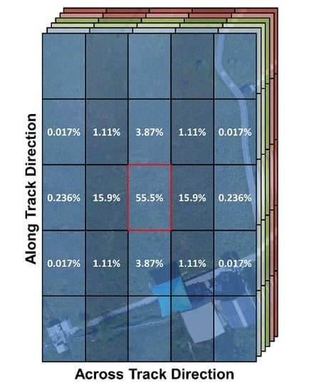
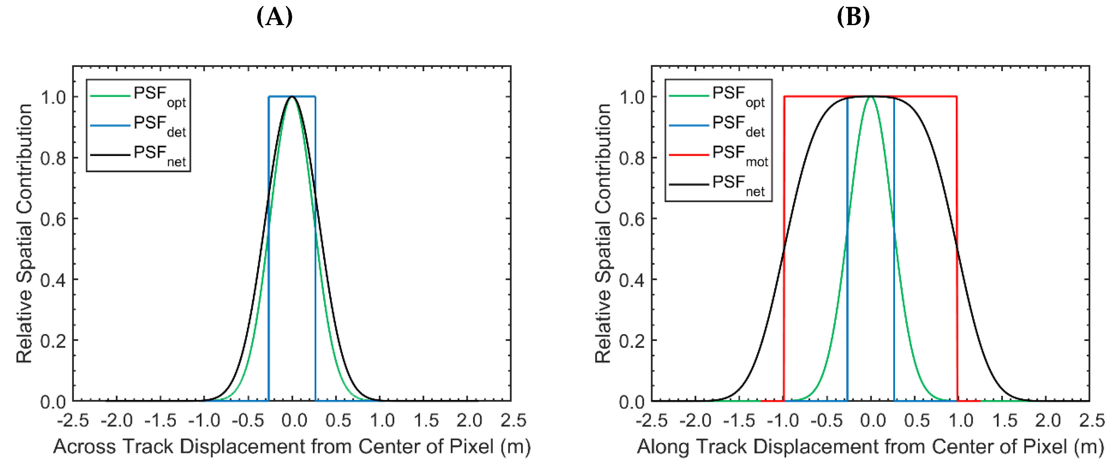
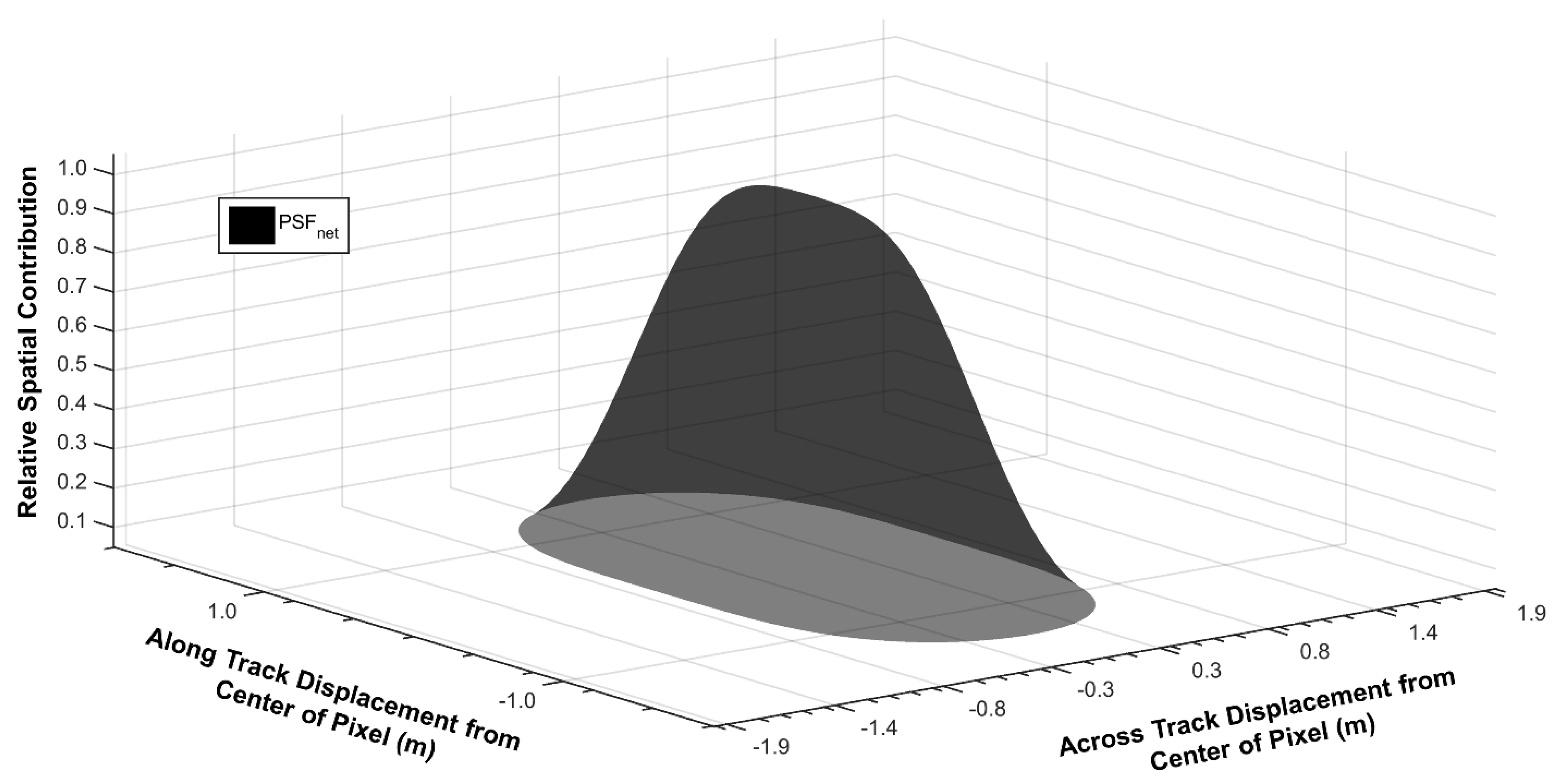
2.2. Deriving the Theoretical Point Spread Function for each CASI Pixel

The theoretical PSF_net was calculated separately in the across track and along track directions. The derivation relied on 2 assumptions: (1) the aircraft was flying at a constant altitude, speed and heading with 0 roll and pitch; (2) the aircraft flight line was perpendicular to the detector array. With the sensor properties and the flight parameters of the Mer Bleue imagery (Table 1), the GIFOV of the CASI was calculated to be 0.55 m in both the along track and the across track directions. The PSF_opt was derived from a Gaussian function with a full-width at half-maximum of 1.1 detector array pixels (value provided by sensor manufacturer) in both the across track and along track directions. The PSF_net in the across track direction was derived by convolving the PSF_opt with the PSF_det, which was a rectangular pulse function with a width equal to the GIFOV (Figure 2A). The PSF_net in the along track direction was calculated based on the same optical and detector point spread function as in the across track direction. The PSF_mot in the along track was approximated by a rectangular pulse function with a width equal to the along track pixel spacing or, equivalently, the nominal ground speed of the sensor (41.5 m/s) multiplied by the integration time (48 ms) for each line. No electronic filters were applied to the CASI data during data acquisition and thus the dynamics of the PSF_electronic were not considered. The PSF_net in the along track was calculated by convolving the detector, optical, and motion point spread functions (Figure 2B). The total PSF_net was derived by multiplying the PSF_net in the across track and along track directions (Figure 3). Based on this derivation, the pixel resolution of the CASI imagery was approximately 0.55 m and 1.99 m in the across track and along track directions, respectively.

2.3. Simulated HSI Data

To investigate the implication of sensor induced blurring, the study simulated two hyperspectral images at the same approximate spatial resolution of the Mer Bleue CASI dataset (0.55 m in the across track and 1.99 m in the along track). The two artificial images were only distinguished by the simulated sensor blurring. The first image (referred to as the ideal image) represented an ideal scenario where the PSF_net was uniform across the spatial boundaries of each pixel. The PSF_net of the second image (referred to as the non-ideal image) was modelled after the derived spatial response of the CASI.

Both datasets were derived from an image that was designed to represent a vegetation plot within the Mer Bleue Peatland at a spatial resolution 50 times finer than that of the real-world CASI data. The value for each spectral band and spatial pixel in the high spatial resolution imagery was randomly generated from a normal distribution. The mean and standard deviation of the normal distribution for each band were derived from the basic statistics of a 3660–pixel vegetation region of interest (Figure 4) from the original Mer Bleu CASI imagery. All the pixels within the region of interest were examined to ensure that vegetation was not contaminated by any man-made structures or objects. The mean value of each spectral band from the vegetation region of interest in the Mer Bleue CASI imagery was used as the mean value of the normal distribution for each band. Due to the change in scale between the pixels within the high spatial resolution imagery and the real-world CASI imagery, the calculated standard deviation needed to be scaled up by a factor of 50 before it could be used as the standard deviation in the normal distribution.

To simulate the ideal and non-ideal images from the generated high spatial resolution imagery, the derived PSF_net function (Section 2.2 of the Methodology) was convolved with the high spatial resolution imagery and spatially resampled to the native resolution of the CASI imagery using a nearest-neighbour resampling approach. The nearest neighbour resampling approach was equivalent to directly downsampling the convolved data by a factor of 50 to the native resolution of the CASI imagery. Given the described simulation process, 100% of the information content was known for both the ideal and non-ideal datasets and the environment that they represented. The mean and standard deviation for each spectral band within the two simulated images were calculated to assess the implication of sensor induced blurring effects on the global statistics of the simulated HSI data. When comparing the mean of the spectra from two different images, a t-test with unequal variances was applied separately for each spectral band. The mean spectra from the two compared images at a particular band were deemed significantly different if the p-value was less than 0.05. When comparing the standard deviation (and, in extension, variance) in the spectra from two different images, an F-test for equal variances was applied separately for each spectral band. The standard deviation in the spectra from the compared images at a particular band were deemed significantly different if the p-value was less than 0.05.

2.4. Visualizing and Quantifying Spatial Correlations

For an ideal sensor, the spatial correlations within HSI data are piece-wise smooth, meaning that neighbouring pixels are highly correlated [5]. This correlation structure can be leveraged to quantify sensor-generated spatial correlations with a correlation metric. The Pearson product-moment correlation coefficient (CC) has been shown as a strong tool in the analysis of HSI data [56]. The CC is a measure of linear association between two variables. It is formally given [57] by the following equation:

$$CC=\frac{{\displaystyle \sum }\left(A_i-\overline{A}\right)\left(B_i-\overline{B}\right)}{\sqrt{{\displaystyle \sum }{\left(A_i-\overline{A}\right)}^2{\displaystyle \sum }{\left(B_i-\overline{B}\right)}^2}},$$

(7)

where $A_i$, $B_i$,$\overline{A}$,$\overline{B}$ represent the two variables of interest and their means, respectively.

The CC was implemented to characterize the spatial structure of correlations in the HSI data. In particular, the correlation coefficient was calculated between the spectra of adjacent pixels in both the across track and along track directions. This process was repeated for distant neighbors. The calculated correlation coefficients were grouped by pixel displacement separately in the across track and along track. The mean and standard deviation of each group was calculated to quantify the strength and variability of the spatial correlations within each image as a function of pixel displacement. This algorithm fundamentally represents the horizontal and vertical cross-section of an autocorrelation function with characterized variability.

2.5. Mitigating Sensor Generated Spatial Correlations Using the PSF_net

A simple deconvolution algorithm was developed to mitigate sensor-generated blurring effects in HSI data. The approach utilizes the theoretically derived PSF_net to mitigate contributions from the materials within the spatial boundaries of neighbouring pixels. Let S_0,0 represent the reflectance spectrum of any given pixel in an ungeocorrected HSI dataset that is contaminated by sensor-generated blurring effects. Let S_i,j represent the spectrum from the pixel displaced by i rows and j columns from the pixel of interest. Let a_i,j represent the weighted contribution of S_i,j to S_0,0, as calculated by integrating the PSF_net over the spatial boundaries of the pixel from which S_i,j originated. By removing the relative contribution of all neighbouring pixels from S_0,0, it is possible to generate a new approximation, ${\widehat{S}}_{0,0}$, in which sensor-generated blurring effects have been mitigated:

$${\widehat{S}}_{0,0}=\frac{S_{0,0}-{\sum }_{i\in Z/i\ne 0}{\sum }_{j\in Z/j\ne 0}{a}_{i,j}{S}_{i,j}}{a_{0,0}}$$

(8)

The algorithm assumes sub-pixel materials are homogenous. Furthermore, neighbouring pixels are assumed to be unaffected by sensor blurring effects. Similar assumptions have been made in other deconvolution studies (e.g., [26,58]). Although these assumptions may not be realistic for real-world spectral imagery, they are reasonable to simplify the system as the spatial variability within each pixel is often non-constant and unknown.

2.6. Algorithm Application to Simulated HSI Data

The developed algorithms were applied to the simulated datasets. In particular, the spatial correlation structure of the two simulated images were characterized by the CC based algorithm. The algorithm was assessed based on its ability to detect discrepancies in the spatial correlation structure. The deconvolution algorithm was implemented by applying Equation (8) to the simulated dataset with a non-ideal PSF_net. The deconvolved dataset was referred to as the corrected non-ideal image. The deconvolution algorithm was assessed based on its ability to recover the global statistics of the ideal imagery from the non-ideal imagery. The deconvolution algorithm was also evaluated based on its ability to restore the spatial correlation structure observed in the ideal image by the CC based algorithm. The study used the same statistical tests as in Section 2.3 (t-test with unequal variances and f-test for equal variances) when comparing the mean and standard deviation of the spectra between the two images within the vegetation region of interest. To ensure that the observed trends in global statistics were actually linked to a decrease of difference between the ideal and non-ideal image after the application of the deconvolution algorithm, Euclidean distance was calculated on a pixel-by-pixel basis between the ideal imagery and both the non-ideal and corrected non-ideal images.

2.7. Algorithm Application to Real-World HSI Data

The developed algorithms were applied to the collected HSI data at the Mer Bleue peatland and the calibration site at the airport with a primary focus on the deconvolution algorithm. Image sharpness was assessed by calculating the slope of a horizonal profile across image structures with sharp edges that separated two materials with distinct spectral signatures. In the Mer Bleue image, the edge of the grey calibration tarp was analyzed. In the airport imagery, the edge along the border of a concrete-asphalt transition was used. The CC based algorithm was then applied to vegetation within the Mer Bleue image to assess the correlation structure of the images before and after the application of the deconvolution algorithm. The mean and standard deviation in each spectral band of the Mer Bleue imagery within the vegetation region of interest was calculated before and after the application of the deconvolution algorithm. The study used the same statistical tests as in Section 2.3 (t-test with unequal variances and f-test for equal variances) when comparing the mean and standard deviation of the spectra between the two images within the vegetation region of interest.

3. Results

3.1. Theoretical Point Spread Function for Each CASI Pixel

The total PSF_net was Gaussian in nature, with a maximum value at the origin, dropping off rapidly to approximately zero past a distance of 2 m (~1 pixel) in the along track and 1 m in the across track (~2 pixels) directions. Figure 5 displays the relative contribution to the spectrum from a single pixel. Only 55.5% of the signal from each pixel originated from the materials within its spatial boundaries. Neighbouring contributions in the across track were larger than in the along track.

3.2. Simulated HSI Data

Panels A and B in Figure 6 display the ideal and non-ideal simulated hyperspectral images, respectively. The mean and standard deviation of each spectral band from the ideal and non-ideal images are shown in Figure 7. The mean values for each spectral band between the two simulated datasets were not significantly different (two-sample t-test with unequal variances applied separately for each spectral band; p-values > 0.792). In fact, the mean spectra were essentially identical, with an extremely small root-mean-square deviation (0.004%) relative to the range of the data (28.2%). The variances between the two simulated datasets for each spectral band were significantly different (F-test for equal variances applied separately for each spectral band; p-values < 1.29E–26). The standard deviation in each spectral band of the non-ideal simulated dataset were 31.1%–38.9% smaller when compared to the ideal imagery.

3.3. Algorithm Application to Simulated HSI Data

The results of the CC based method when applied to the ideal and non-ideal imagery are displayed in Figure 8. The figures also display the results of the CC based method when applied to the non-ideal imagery after using the developed deconvolution algorithm (referred to as the corrected non-ideal image). The corrected non-ideal image can be seen in panel C of Figure 6. In the ideal simulated imagery, the mean of each group was relatively constant at a value of ~0.982 for all pixel displacements in both the across track and along track directions. Similarly, the standard deviation around the mean was also constant at a value of ~0.002. For pixel displacements >1, the mean and standard deviation of each CC group in the non-ideal imagery was relatively constant at a value of 0.992 and 0.001, respectively. This trend held for both the across track and along track directions. For a pixel displacement value of 1, the mean CC was relatively large, at a value of 0.996 and 0.993 in the across track and along track directions, respectively. The corresponding standard deviations around these mean values were relatively small, at 0.0006 and 0.0008. The standard deviation in the calculated CCs for the non-ideal simulated dataset were 54.0%–75.4% smaller when compared to the ideal imagery.

The mean CC for each group in the corrected non-ideal image were similar in magnitude to the ideal image. For the corrected image in the along track direction, the mean and standard deviation of each CC group was relatively constant at values of 0.981 and 0.002, respectively. This trend held for pixel displacements > 2 in the across-track. The mean CC for pixels displaced by 1 in the across track direction was relatively large (0.984). The opposite trend was observed for pixel displacements of 2 in the across-track, with a mean value of 0.978 and a standard deviation of 0.003. The standard deviation in the CCs of the corrected non-ideal image were within 23.3% of the values calculated for the ideal image.

The mean and standard deviation of each spectral band in the corrected non-ideal image were almost identical to those of the ideal image; there was no significant difference in the mean (two-sample t-test with unequal variances applied separately for each spectral band; p-values > 0.825) or variance (F-test for equal variances applied separately for each spectral band; p-values > 0.056). The mean spectra were essentially identical, with an extremely small root-mean-square deviation (0.004%) relative to the range of the data (28.2%). Similarly, the variability in each spectral band of the ideal and corrected non-ideal images were essentially identical, given the small root-mean-square deviation (0.03%) in the standard deviation relative to the range in the data (2.4%) (Figure 9). The standard deviations in each spectral band of the corrected non-ideal image were within 6.8% of the values calculated for the ideal image. The Euclidean distance (in units of reflectance) between the ideal imagery and both the non-ideal and corrected non-ideal images are displayed in Figure 10A,B, respectively. After the application of the deconvolution algorithm, the Euclidean distance between the ideal and non-ideal imagery decreased by an average of 1.91%.

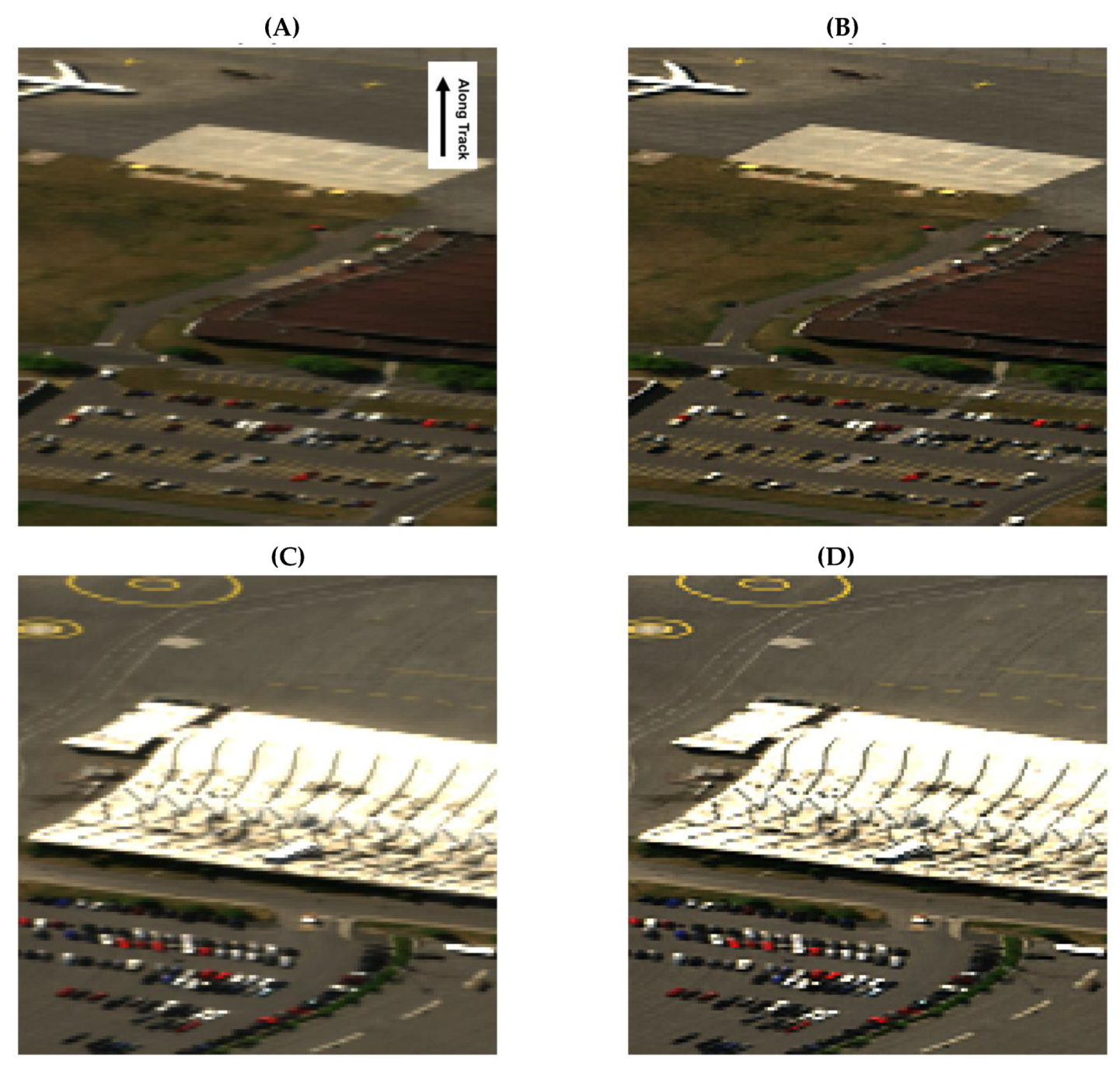
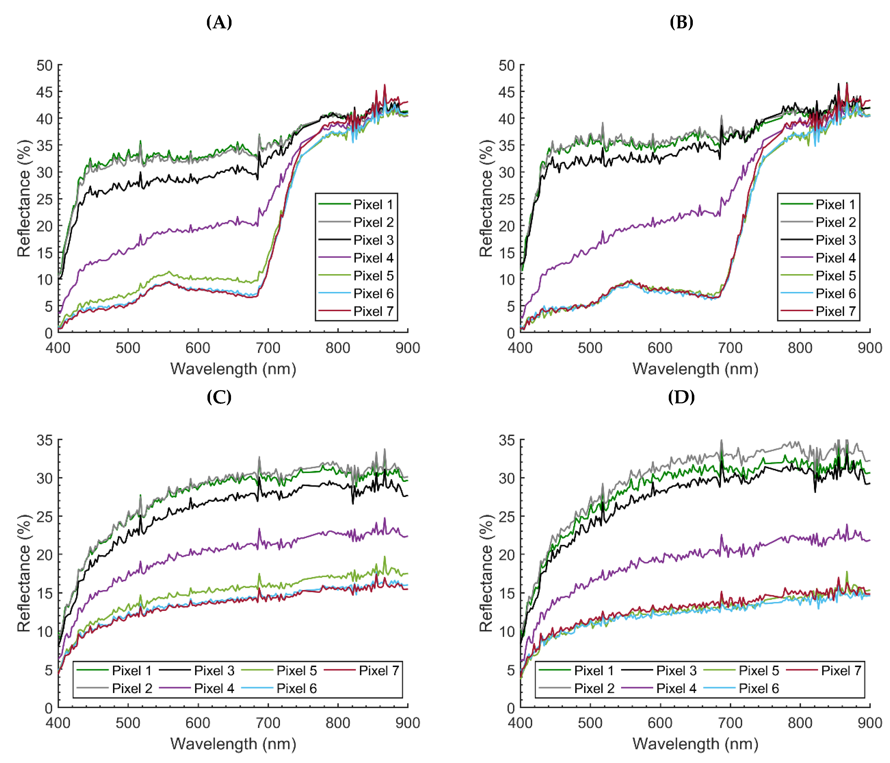
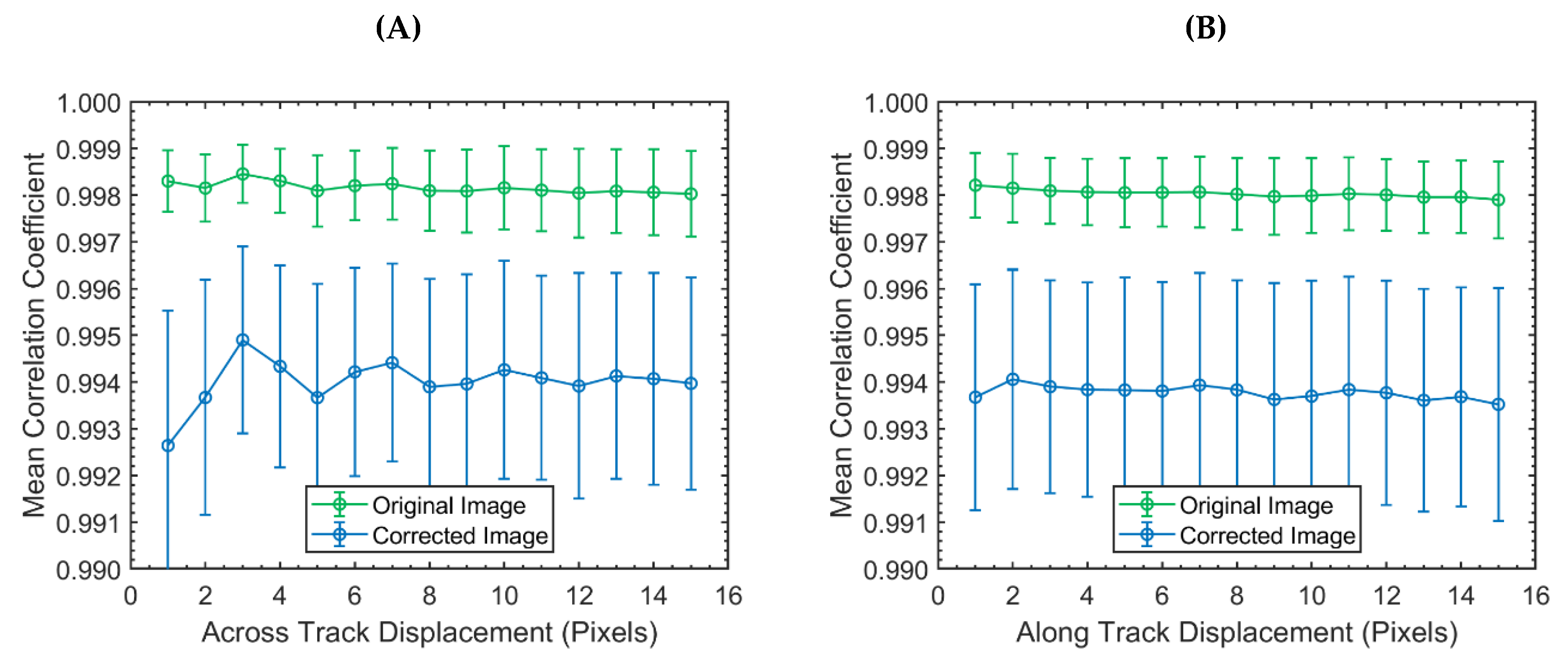
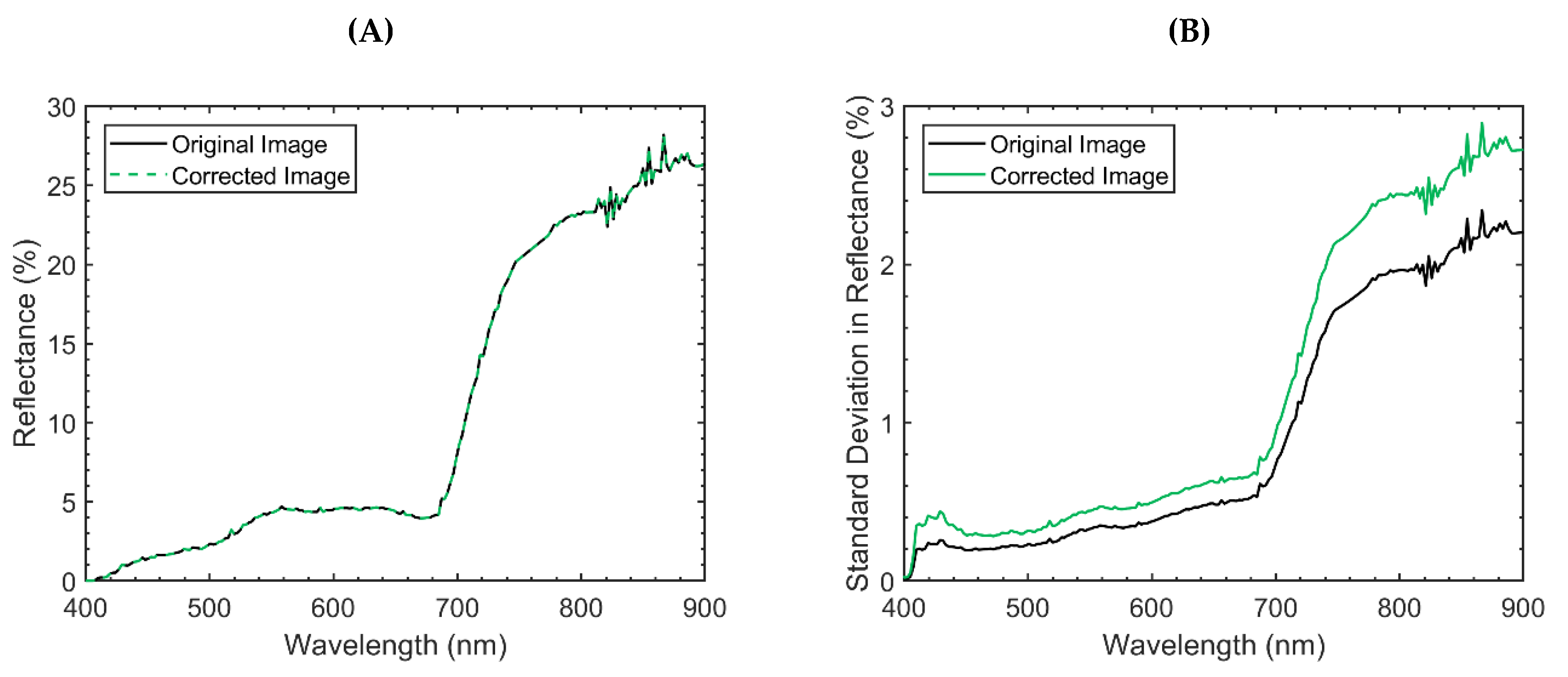
3.4. Algorithm Application to Real-World HSI Data

After applying the deconvolution algorithm to the HSI data, both images were qualitatively sharper (Figure 11 and Figure 12). The spectrum from the 7 adjacent across track pixels for each of the studied edges in the Mer Bleue and Airport imagery were displayed in Figure 13. Pixel 4 was the closest to the studied edge. The pixel number represents the order of each adjacent pixel in the across track direction. In plots A and B, pixels 1–3 represented spectra from the calibration tarp while pixels 5–7 represented spectra from vegetation at the Mer Bleue Peatland. In plots C and D, pixels 1–3 represented spectra from the concrete while pixels 5–7 represented spectra from asphalt from the airport. Plots A and C are from the original imagery, while plots B and D are from the deconvolved imagery. In both the Mer Bleue and Airport imagery, the spectra from pixels 3 and 5 were closer to the spectra of their respective materials after the application of the deconvolution algorithm. In particular, the spectrum from pixel 5 dropped in magnitude, aligning with that of pixels 6 and 7 in both sets of imagery. Quantitatively, the deconvolution algorithm increased the maximum change in reflectance per pixel across the two studied edges by a relatively constant factor of 1.4 (Figure 14).

When applying the CC based algorithm to the vegetation region of interest from the CASI data, there were several differences in the correlation structure between the imagery before and after the application of the deconvolution algorithm (Figure 15). Most notably, the algorithm decreased correlation levels in both the across track and along track directions from 0.998 to 0.994 while increasing the standard deviation in the system approximately by a factor of 3. In the along track direction, spatial correlations decreased marginally along with pixel displacement. This trend held in the across-track, however, there was also a sinusoidal trend that repeated every four pixels (~2 m). This sinusoidal feature dampened by a pixel displacement of 5 in the original imagery. In the corrected imagery, this sinusoidal structure was far more prominent, dampening at a pixel displacement of 12.

The mean and standard deviation of the vegetation plot in the original and corrected imagery is displayed in Figure 16. The mean values for each spectral band between the original and corrected image within the vegetation pixels were not significantly different (two-sample t-test with unequal variances applied separately for each spectral band; p-values > 0.855). The mean spectra were essentially identical, with an extremely small root-mean-square deviation (<0.0035%) relative to the range of the data (31.2%). The variances between the two simulated datasets for each spectral band were significantly different (F-test for equal variances applied separately for each spectral band; p-values < 6.143E–37).

4. Discussion

The objective of this study was to characterize and mitigate sensor-generated blurring effects in airborne HSI data with simple and intuitive tools, emphasizing the importance of point spread functions. By studying the derived CASI PSF_net it was possible to understand the potential implications of sensor induced blurring effects in general.

The CASI PSF_net was roughly Gaussian in shape, extending two pixels in the across track and one pixel in the along track before reaching a value of approximately zero. The spread of this function meant that approximately 45% of the signal in the spectrum from each CASI pixel originated from materials within the spatial boundaries of neighboring pixels (Figure 5). Although these values may seem quite large, it is important to recognize that they are not unreasonable for all imaging spectrometers. For instance, based on the 2D Gaussian PSF_net (full-width at half-maximum of 28 m in the across track and 32 m in the along track [33]) for each Landsat 8 Operational Land Imager pixel (bands 1–7), only 55.5% of the signal originates from materials within the spatial boundaries of each pixel. This value is almost identical to that of the CASI.

With the ideal (perfectly uniform PSF_net over pixel boundaries) and non-ideal (CASI PSF_net) simulated images, the effects of sensor induced blurring could be quantified. From the basic second-order image statistics, sensor induced blurring reduced the spectral variability, as measured by the standard deviation, in the simulated scene by 31.1%–38.9% for all spectral bands. Given the importance of second-order statistics in the analysis of high dimensional data [59], the change in standard deviation exemplifies the information loss associated with sensor blurring. The CC based method further investigated this loss of information, while verifying the detective and corrective capabilities of the developed algorithms.

The CASI PSF_net modified the spatial correlation structure of the image. In particular, spatial correlations substantially increased for closely neighbouring pixels displaced by 2 in the across track and 1 in the along track. These results directly reflect the structure of the CASI PSF_net. Although the PSF_net did not extend spatially more than 2 pixels, spatial correlations were saturated for all pixel displacements. These saturated correlations showcase that local sensor blurring can have global impacts on HSI data.

The standard deviation in the calculated CCs indicated that sensor induced blurring attenuated the natural spatial variability in the image. Once again, this trend held on a global scale but was more prominent locally. In fact, sensor induced blurring reduced the variability, as measured by the standard deviation, in the spatial correlation structure of the imaged scene by 54.0%–75.4% for all pixel displacements. As expected, these findings suggest that sensor generated spatial correlations act to mask and distort the spatial dynamics of the imaged scene while removing natural variations.

It is important to note that, despite only observing deviations in the CCs from the 3rd–4th decimal places, the CC based method was still sensitive to the simulated blurring effects, especially the saturated correlations and the asymmetry between the across track and along track spatial correlations. With this in mind, the CC based algorithm can be applied to assess the effectiveness of deconvolution algorithms that attempt to mitigate sensor-generated spatial correlations. This was exemplified by the developed deconvolution algorithm.

When applied to the non-ideal dataset, the deconvolution algorithm brought the spectral variability, as measured by the standard deviation, within 6.8% of the spectral variability in the ideal image. In fact, there was no significant difference in the spectral variance between the ideal and corrected non-ideal datasets. This finding suggests that the deconvolution algorithm recovered some of the information that was attenuated by sensor blurring. A closer examination of the algorithm’s performance with the CC based method revealed similar conclusions.

In the corrected non-ideal image, the standard deviation values around the calculated mean CCs were relatively constant, similar in magnitude to those observed in the ideal simulated image. In fact, the spatial structure in the along track of the ideal image was almost completely recovered from the non-ideal image. A similar statement can be made in the across track for pixel displacements > 2. Although the algorithm decreased the mean CC for neighbouring pixels separated by < 3 in the across-track, it did not completely restore the spatial structure. At a pixel displacement of 1, there were still elevated correlation levels. In addition, the algorithm introduced an artificial decorrelation at a pixel displacement of 2 in the across-track. This decorrelation was a consequence of the pure pixel assumption. Although these artifacts may be problematic for some applications, it is important to recognize that deconvolution is an ill-posed problem; information will always be lost in a blurred image and thus it is impossible to perfectly eliminate sensor blurring effects, especially at the attenuated high frequencies [31]. In fact, many algorithms suffer from difficulties in restoring high-frequency spatial structures in HSI data [45]. Despite introducing this decorrelation, the equalized spatial correlation levels revealed that the algorithm restored the spatial structure of the dataset to some degree. A similar conclusion could be drawn from the standard deviation of the calculated CC values. The deconvolution algorithm brought the variability in the spatial correlation structure of the non-ideal imagery within 23.3% of the spatial variability in the ideal imagery.

To ensure that the increase of spatial and spectral variability was linked to a decrease of difference between the ideal and non-ideal simulated images, Euclidean distance metrics were calculated. As shown in Figure 10, the Euclidean distance between the ideal and non-ideal imagery decreased by an average of 1.91% after the application of the deconvolution algorithm. Along with these findings, the increased spectral and spatial variability continue to suggest that the simple deconvolution algorithm is restoring some of the information that was lost to sensor blurring.

To assess the deconvolution algorithm further, it was applied to real-world HSI data. When applied to both real-world HSI datasets, there was a qualitative increase in image sharpness (Figure 11 and Figure 12). In the airport imagery, this was evident from the abundant high contrast edges produced by man-made structures like roads, buildings, cars, and parking lots. Although there were fewer high contrast materials in the Mer Bleue imagery, the calibration tarps and tree crowns clearly showcased the sharpening effect of the deconvolution algorithm. These observations were supported quantitatively by analyzing the edge of a calibration tarp in the Mer Bleue imagery and the edges of the calibration site in the airport imagery. In Figure 13, the spectra of the adjacent 7 pixels to each of the studied edges were displayed. In both the Mer Bleue and Airport imagery, the spectra from the pixels immediately neighbouring the edge pixel were closer to the spectra of their respective materials after the application of the deconvolution algorithm, indicating that the imagery had been sharpened. This finding was supported by Figure 14, where the horizontal profile across the two edges increased in slope (an in extension image sharpness) by an approximate factor of 1.4 after the application of the deconvolution algorithm.

To showcase an application of the developed algorithms, the CC based method was applied to the vegetation region of interest (Figure 4) in the Mer Bleue image to analyze the spatial correlation structure of the plot before and after the deconvolution was applied. In the original imagery, spatial correlations decreased marginally over space in both the across track and along track. This decrease likely corresponded with changes in the peatland over large spatial scales. With a priori knowledge of the micro spatial patterns in the vegetation and surface elevation (Figure 1) [24,49,50,54], it was possible to observe a subtle sinusoidal structure in the correlation plots that repeated every 4 pixels (2 m) in the across-track. The period of this sinusoidal structure agreed with the spatial scale of the patterns in surface vegetation and microtopography (2–4m) [51,52,53]. These trends were not apparent in the along track. However, this was to be expected based on the Nyquist sampling theorem; the sampling frequency in the along track direction (0.5 cycles per m) was less than the frequency of the patterns in surface vegetation and microtopography (0.25–0.5 cycles per m) multiplied by 2 and thus undetectable. After applying the deconvolution algorithm, there was an overall decrease in the spatial correlations. The simulation results suggested that this decrease was due to the attenuation of sensor induced correlations. The sinusoidal structure in the across track was more prominent after the deconvolution algorithm was applied. These results suggest that the deconvolution algorithm highlighted the patterns in microtopography and, in extension, vegetation composition. In this particular ecosystem, the microtopography is important as it covaries with surface vegetation, water table position, and carbon uptake from the atmosphere [52].

Although more sophisticated deconvolution algorithms exist [31,44,45,46], they may rely on a higher level of mathematical understanding to implement. Without a fundamental understanding of a method, its implementation can lead to inaccurate interpretations. This may be problematic for end-users, who often do not have the appropriate information to implement these methodologies effectively. The presented method is intuitive; the algorithm is based on the principles of the classical linear spectral unmixing model and is thus simple to understand and implement. Despite using a wavelength-independent PSF_opt that was derived based on a theoretical calculation as opposed to an empirical estimation, the algorithm was capable of sharping real-world HSI data. With a more rigorous characterization of the optical blurring that accounts for the wavelength dependence of the point spread function, the performance of the deconvolution algorithm could be improved, resulting in sharper imagery and a spatial correlation structure more representative of the imaged scene.

Before applying the developed deconvolution algorithm, it is critical to consider the implications and validity of the pure pixel assumption made in Equation 8. Given that HSI may be characterized by sensor blurring and noise that varies as a function of wavelength, these assumptions may not be realistic for real-world spectral imagery. They are, however, reasonable to simplify the system since the spatial variability within each pixel is often non-constant and unknown. Similar pure pixel assumptions have been made in other deconvolution studies (e.g., [26,58]) at the satellite level. This is encouraging since the pure pixel assumption is more likely to hold for airborne systems that collect data at higher spatial resolution (<3 m). That being said, end-users must be aware that the assumption may lead to anomalies in the deconvolved data.

As previously mentioned, the pure pixel assumption resulted in artificial decorrelations at pixel displacements from 1–2 pixels in the across-track. Such artifacts are potentially problematic for certain applications, likely showing overestimated contrast along edges. Despite this, the real-world imagery was sharpened with promising results. When analyzing the sharpening effects on a pixel-by-pixel basis (Figure 13), there was little evidence that showed any overestimated contrast in the imagery. That being said, given the construction of the algorithm, overestimated contrast is possible. Furthermore, this algorithm has no constraints on the positivity of the deconvolved imagery. Since negative reflectance has no real-world significance, edges between extremely high reflectance and low reflectance materials may need to be checked for non-positive anomalies. Furthermore, low signal and excessive noise in the data may negatively affect the performance of the algorithm, also resulting in negative values. As such, the application of this algorithm may not be ideal for low signal to noise ratio bands.

This work focused on developing a simplistic approach to deconvolution, which is a complex and ill-posed problem. To satisfy this objective, the pure pixel assumption was necessary, despite the potential for introducing data anomalies. In this study, there is ample evidence to suggest that the algorithm is effective at mitigating sensor-generated blurring effects within the data. With this in mind, if sensor blurring is the major obstacle for a particular application, the developed methodologies should be sufficient to observe noticeable improvements. From that point, more complex deconvolution algorithms (e.g., [31,44,45,46]) can be implemented if the developed algorithm is introducing too many artifacts in the HSI data.

From both the simulated and real-world HSI data, sensor induced blurring effects were found to mask and distort the natural spatial dynamics of the imaged scene. These blurring effects directly corresponded with the structure of the PSF_net. From this work, it is clear that sensor induced blurring effects are not always identical in the across track and along track directions. The same can be said for the raw pixel sizes. In fact, for pushbroom sensors, pixels are inherently more rectangular than square. Although it is possible to obtain nearly identical pixel resolutions in the across track and along track directions, technical restraints may make it difficult. For instance, the resolution in the along track is determined by the integration time and platform speed, both of which have impacts on other aspects of the data (signal to noise ratio, positional accuracy, etc.), especially for low altitude platforms such as unmanned aerial systems [60]. This implies that HSI data characterize the scene on a slightly different scale in the across track than the along track directions, with different blurring levels. Given the scale-dependent nature of many natural phenomena, patterns could be observable in one spatial dimension, but not the other. This was exemplified by the Mer Bleue imagery, in which the micro-spatial patterns in surface vegetation could be detected in the across-track, but not the along track. Without considering the PSF_net and the heading of the data acquisition flight, sensor induced blurring effects could be mistaken for directional trends in the data. Similarly, scale-dependent phenomena observable in either the across track or along track directions could lead to assumptions of directionality to a trend where none exists.

Given the importance of sensor point spread functions, when applying HSI data, it may be critical to analyze the imagery in its original sensor geometry, pre-geocorrection. Many geocorrective methods operate by resampling the raw HSI data on a linear grid with a nearest neighbour resampling technique [61]. As such, the location of each point in the raw imagery is shifted and the original sensor geometry is lost to some degree. Consequently, the natural spatial correlations of a scene are likely to be distorted even further as sensor-generated spatial correlations are shifted to fit the pre-specified linear grid. Further research into the spatial correlation structure of HSI data post geocorrection would give insight into the cumulative effects of sensor-generated spatial correlations.

Overall, the described methodology provides a framework to characterize and mitigate the implications of sensor induced blurring; by generating a simulated dataset with known blurring, it is possible to understand the degree to which sensor blurring (and the associated artificial spatial correlations) will affect real-world HSI data. At the satellite level, there exists a rich body of literature that characterizes and discusses the implications of sensor point spread functions on a wide array of remote sensing tasks such as classification [26], sub-pixel feature detection [35], and spectral unmixing [36]. Unfortunately, the implications of sensor point spread functions have yet to be fully investigated to the same degree at the airborne level. This may be problematic as sensor-generated blurring effects may be more prominent for airborne platforms [43].

5. Conclusions

The presented work developed two simple and intuitive algorithms to characterize and mitigate sensor-generated spatial correlations while emphasizing the implications of sensor point spread functions. The first algorithm applied the CC to observe and quantify spatial correlations. The algorithm was able to characterize the structure of spatial correlations. Sensor blurring was found to increase spatial correlations and decrease the variance in the system. The second algorithm developed in the study used a theoretically derived PSF_net to mitigate sensor-generated spatial correlations in HSI data. The CC-based algorithm showed that sensor blurring generated spatial correlations that removed 54.0%–75.4% of the natural variability in the spatial correlation structure of the simulated HSI data. Sensor blurring effects were also shown to remove 31.1%–38.9% of the spectral variability. The deconvolution algorithm mitigated the observed sensor-generated spatial correlations while restoring a large portion of the natural spectral and spatial variability of the scene. In the real-world I data, the deconvolution algorithm quantitatively and qualitatively sharpened the imagery, decreasing levels of spatial correlation within the imagery that were likely caused by sensor induced blurring effects. As a result of this effect, the natural spatial correlations within the imagery were enhanced. The presented work substantiates the implications of sensor-generated spatial correlations while providing a framework to analyze the implications of sensor blurring for specific applications. Point spread functions are shown to be crucial variables to complement traditional parameters such as pixel resolution and geometric accuracy. The developed tools are simple and intuitive. As a result, they can be readily applied by end-users of all expertise levels to consider the impact of sensor-generated blurring, and by extension, spatial correlations, HSI applications.

References

1. Green, R.O.; Eastwood, M.L.; Sarture, C.M.; Chrien, T.G.; Aronsson, M.; Chippendale, B.J.; Faust, J.A.; Pavri, B.E.; Chovit, C.J.; Solis, M. Imaging spectroscopy and the airborne visible/infrared imaging spectrometer (AVIRIS). Remote Sens. Environ. 1998, 65, 227–248. [Google Scholar] [CrossRef]
2. Cocks, T.; Jenssen, R.; Stewart, A.; Wilson, I.; Shields, T. The HyMapTM airborne hyperspectral sensor: The system, calibration and performance. In Proceedings of the 1st EARSeL Workshop on Imaging Spectroscopy, Zurich, Switzerland, 6–8 October 1998; pp. 37–42. [Google Scholar]
3. Babey, S.; Anger, C. A compact airborne spectrographic imager (CASI). In Proceedings of the IGARSS ’89 Quantitative Remote Sensing: An Economic Tool for the Nineties, New York, NY, USA, 10–14 July 1989; Volume 2, pp. 1028–1031. [Google Scholar]
4. Pearlman, J.S.; Barry, P.S.; Segal, C.C.; Shepanski, J.; Beiso, D.; Carman, S.L. Hyperion, a space-based imaging spectrometer. IEEE Trans. Geosci. Remote Sens. 2003, 41, 1160–1173. [Google Scholar] [CrossRef]
5. Bioucas-Dias, J.M.; Plaza, A.; Camps-Valls, G.; Scheunders, P.; Nasrabadi, N.; Chanussot, J. Hyperspectral Remote Sensing Data Analysis and Future Challenges. IEEE Geosci. Remote Sens. Mag. 2013, 1, 6–36. [Google Scholar] [CrossRef] [Green Version]
6. Eismann, M.T. 1.1 Hyperspectral Remote Sensing. In Hyperspectral Remote Sensing; SPIE: Bellingham, WA, USA, 2012. [Google Scholar]
7. Berk, A.; Anderson, G.P.; Bernstein, L.S.; Acharya, P.K.; Dothe, H.; Matthew, M.W.; Adler-Golden, S.M.; Chetwynd Jr, J.H.; Richtsmeier, S.C.; Pukall, B. MODTRAN4 radiative transfer modeling for atmospheric correction. In Proceedings of the Optical Spectroscopic Techniques and instrumentation for atmospheric and space research III, Denver, CO, USA, 18–23 July 1999; pp. 348–353. [Google Scholar]
8. Cloutis, E.A. Review article hyperspectral geological remote sensing: Evaluation of analytical techniques. Int. J. Remote Sens. 1996, 17, 2215–2242. [Google Scholar] [CrossRef]
9. Murphy, R.J.; Monteiro, S.T.; Schneider, S. Evaluating classification techniques for mapping vertical geology using field-based hyperspectral sensors. IEEE Trans. Geosci. Remote Sens. 2012, 50, 3066–3080. [Google Scholar] [CrossRef]
10. van der Meer, F.D.; van der Werff, H.M.A.; van Ruitenbeek, F.J.A.; Hecker, C.A.; Bakker, W.H.; Noomen, M.F.; van der Meijde, M.; Carranza, E.J.M.; Smeth, J.B.d.; Woldai, T. Multi- and hyperspectral geologic remote sensing: A review. Int. J. Appl. Earth Obs. Geoinf. 2012, 14, 112–128. [Google Scholar] [CrossRef]
11. Yao, H.; Tang, L.; Tian, L.; Brown, R.; Bhatnagar, D.; Cleveland, T. Using hyperspectral data in precision farming applications. Hyperspectral Remote Sens. Veg. 2011, 1, 591–607. [Google Scholar]
12. Dale, L.M.; Thewis, A.; Boudry, C.; Rotar, I.; Dardenne, P.; Baeten, V.; Pierna, J.A.F. Hyperspectral imaging applications in agriculture and agro-food product quality and safety control: A review. Appl. Spectrosc. Rev. 2013, 48, 142–159. [Google Scholar] [CrossRef]
13. Migdall, S.; Klug, P.; Denis, A.; Bach, H. The additional value of hyperspectral data for smart farming. In Proceedings of the Geoscience and Remote Sensing Symposium (IGARSS), 2012 IEEE International, Munich, Germany, 22–27 July 2012; pp. 7329–7332. [Google Scholar]
14. Koch, B. Status and future of laser scanning, synthetic aperture radar and hyperspectral remote sensing data for forest biomass assessment. ISPRS J. Photogramm. Remote Sens. 2010, 65, 581–590. [Google Scholar] [CrossRef]
15. Peng, G.; Ruiliang, P.; Biging, G.S.; Larrieu, M.R. Estimation of forest leaf area index using vegetation indices derived from hyperion hyperspectral data. IEEE Trans. Geosci. Remote Sens. 2003, 41, 1355–1362. [Google Scholar] [CrossRef] [Green Version]
16. Smith, M.-L.; Martin, M.E.; Plourde, L.; Ollinger, S.V. Analysis of hyperspectral data for estimation of temperate forest canopy nitrogen concentration: Comparison between an airborne (AVIRIS) and a spaceborne (Hyperion) sensor. IEEE Trans. Geosci. Remote Sens. 2003, 41, 1332–1337. [Google Scholar] [CrossRef]
17. Kruse, F.A.; Richardson, L.L.; Ambrosia, V.G. Techniques developed for geologic analysis of hyperspectral data applied to near-shore hyperspectral ocean data. In Proceedings of the Fourth International Conference on Remote Sensing for Marine and Coastal Environments, Orlando, FL, USA, 17–19 March 1997; p. 19. [Google Scholar]
18. Chang, G.; Mahoney, K.; Briggs-Whitmire, A.; Kohler, D.; Mobley, C.; Lewis, M.; Moline, M.; Boss, E.; Kim, M.; Philpot, W. The New Age of Hyperspectral Oceanography. Oceanography 2004, 17, 16–23. [Google Scholar] [CrossRef] [Green Version]
19. Ryan, J.P.; Davis, C.O.; Tufillaro, N.B.; Kudela, R.M.; Gao, B.-C. Application of the hyperspectral imager for the coastal ocean to phytoplankton ecology studies in Monterey Bay, CA, USA. Remote Sens. 2014, 6, 1007–1025. [Google Scholar] [CrossRef] [Green Version]
20. Kalacska, M.; Bell, L. Remote sensing as a tool for the detection of clandestine mass graves. Can. Soc. Forensic Sci. J. 2006, 39, 1–13. [Google Scholar] [CrossRef]
21. Kalacska, M.E.; Bell, L.S.; Arturo Sanchez-Azofeifa, G.; Caelli, T. The application of remote sensing for detecting mass graves: An experimental animal case study from Costa Rica. J. Forensic Sci. 2009, 54, 159–166. [Google Scholar] [CrossRef]
22. Leblanc, G.; Kalacska, M.; Soffer, R. Detection of single graves by airborne hyperspectral imaging. Forensic Sci. Int. 2014, 245, 17–23. [Google Scholar] [CrossRef]
23. Turner, W.; Spector, S.; Gardiner, N.; Fladeland, M.; Sterling, E.; Steininger, M. Remote sensing for biodiversity science and conservation. Trends Ecol. Evol. 2003, 18, 306–314. [Google Scholar] [CrossRef]
24. Arroyo-Mora, J.; Kalacska, M.; Soffer, R.; Moore, T.; Roulet, N.; Juutinen, S.; Ifimov, G.; Leblanc, G.; Inamdar, D. Airborne Hyperspectral Evaluation of Maximum Gross Photosynthesis, Gravimetric Water Content, and CO2 Uptake Efficiency of the Mer Bleue Ombrotrophic Peatland. Remote Sens. 2018, 10, 565. [Google Scholar] [CrossRef] [Green Version]
25. Kalacska, M.; Arroyo-Mora, J.; Soffer, R.; Roulet, N.; Moore, T.; Humphreys, E.; Leblanc, G.; Lucanus, O.; Inamdar, D. Estimating peatland water table depth and net ecosystem exchange: A comparison between satellite and airborne imagery. Remote Sens. 2018, 10, 687. [Google Scholar] [CrossRef] [Green Version]
26. Huang, C.; Townshend, J.R.; Liang, S.; Kalluri, S.N.; DeFries, R.S. Impact of sensor’s point spread function on land cover characterization: Assessment and deconvolution. Remote Sens. Environ. 2002, 80, 203–212. [Google Scholar] [CrossRef]
27. Schowengerdt, R.A. 3.4. Spatial Response. In Remote Sensing: Models and Methods for Image Processing; Elsevier: Amsterdam, The Netherlands, 2006. [Google Scholar]
28. Zhang, Z.; Moore, J.C. Chapter 4—Remote Sensing. In Mathematical and Physical Fundamentals of Climate Change; Zhang, Z., Moore, J.C., Eds.; Elsevier: Boston, MA, USA, 2015; pp. 111–124. [Google Scholar] [CrossRef]
29. Schowengerdt, R.A.; Antos, R.L.; Slater, P.N. Measurement Of The Earth Resources Technology Satellite (Erts-1) Multi-Spectral Scanner OTF From Operational Imagery; SPIE: Bellingham, WA, USA, 1974; Volume 46. [Google Scholar]
30. Rauchmiller, R.F.; Schowengerdt, R.A. Measurement Of The Landsat Thematic Mapper Modulation Transfer Function Using An Array Of Point Sources. Opt. Eng. 1988, 27, 334–343. [Google Scholar] [CrossRef]
31. Chaudhuri, S.; Velmurugan, R.; Rameshan, R. Chapter 2 Mathematical Background. In Blind Image Deconvolution: Methods and Convergence; Springer International Publishing: Madrid, Spain, 2014. [Google Scholar]
32. Hu, W.; Xue, J.; Zheng, N. PSF estimation via gradient domain correlation. IEEE Trans. Image Process. 2012, 21, 386–392. [Google Scholar] [CrossRef] [PubMed]
33. Markham, B.L.; Arvidson, T.; Barsi, J.A.; Choate, M.; Kaita, E.; Levy, R.; Lubke, M.; Masek, J.G. 1.03—Landsat Program. In Comprehensive Remote Sensing; Liang, S., Ed.; Elsevier: Oxford, UK, 2018; pp. 27–90. [Google Scholar] [CrossRef]
34. Markham, B.L. The Landsat sensors’ spatial responses. IEEE Trans. Geosci. Remote Sens. 1985, 6, 864–875. [Google Scholar] [CrossRef]
35. Radoux, J.; Chomé, G.; Jacques, D.C.; Waldner, F.; Bellemans, N.; Matton, N.; Lamarche, C.; d’Andrimont, R.; Defourny, P. Sentinel-2’s potential for sub-pixel landscape feature detection. Remote Sens. 2016, 8, 488. [Google Scholar] [CrossRef] [Green Version]
36. Wang, Q.; Shi, W.; Atkinson, P.M. Enhancing spectral unmixing by considering the point spread function effect. Spat. Stat. 2018, 28, 271–283. [Google Scholar] [CrossRef] [Green Version]
37. Aiazzi, B.; Selva, M.; Arienzo, A.; Baronti, S. Influence of the System MTF on the On-Board Lossless Compression of Hyperspectral Raw Data. Remote Sens. 2019, 11, 791. [Google Scholar] [CrossRef] [Green Version]
38. Bergen, K.M.; Brown, D.G.; Rutherford, J.F.; Gustafson, E.J. Change detection with heterogeneous data using ecoregional stratification, statistical summaries and a land allocation algorithm. Remote Sens. Environ. 2005, 97, 434–446. [Google Scholar] [CrossRef]
39. Simms, D.M.; Waine, T.W.; Taylor, J.C.; Juniper, G.R. The application of time-series MODIS NDVI profiles for the acquisition of crop information across Afghanistan. Int. J. Remote Sens. 2014, 35, 6234–6254. [Google Scholar] [CrossRef] [Green Version]
40. Tarrant, P.; Amacher, J.; Neuer, S. Assessing the potential of Medium-Resolution Imaging Spectrometer (MERIS) and Moderate-Resolution Imaging Spectroradiometer (MODIS) data for monitoring total suspended matter in small and intermediate sized lakes and reservoirs. Water Resour. Res. 2010, 46. [Google Scholar] [CrossRef]
41. Heiskanen, J. Tree cover and height estimation in the Fennoscandian tundra–taiga transition zone using multiangular MISR data. Remote Sens. Environ. 2006, 103, 97–114. [Google Scholar] [CrossRef]
42. Torres-Rua, A.; Ticlavilca, A.; Bachour, R.; McKee, M. Estimation of surface soil moisture in irrigated lands by assimilation of landsat vegetation indices, surface energy balance products, and relevance vector machines. Water 2016, 8, 167. [Google Scholar] [CrossRef] [Green Version]
43. Schlapfer, D.; Nieke, J.; Itten, K.I. Spatial PSF nonuniformity effects in airborne pushbroom imaging spectrometry data. IEEE Trans. Geosci. Remote Sens. 2007, 45, 458–468. [Google Scholar] [CrossRef]
44. Fang, H.; Luo, C.; Zhou, G.; Wang, X. Hyperspectral image deconvolution with a spectral-spatial total variation regularization. Can. J. Remote Sens. 2017, 43, 384–395. [Google Scholar] [CrossRef]
45. Henrot, S.; Soussen, C.; Brie, D. Fast positive deconvolution of hyperspectral images. IEEE Trans. Image Process. 2013, 22, 828–833. [Google Scholar] [CrossRef] [PubMed] [Green Version]
46. Jackett, C.; Turner, P.; Lovell, J.; Williams, R. Deconvolution of MODIS imagery using multiscale maximum entropy. Remote Sens. Lett. 2011, 2, 179–187. [Google Scholar] [CrossRef]
47. Soffer, R.J.; Ifimov, G.; Arroyo-Mora, J.P.; Kalacska, M. Validation of Airborne Hyperspectral Imagery from Laboratory Panel Characterization to Image Quality Assessment: Implications for an Arctic Peatland Surrogate Simulation Site. Can. J. Remote Sens. 2019, 1–33. [Google Scholar] [CrossRef]
48. Lafleur, P.M.; Roulet, N.T.; Bubier, J.; Frolking, S.; Moore, T.R. Interannual variability in the peatland-atmosphere carbon dioxide exchange at an ombrotrophic bog. Glob. Biogeochem. Cycles 2003, 17, 13. [Google Scholar] [CrossRef] [Green Version]
49. Eppinga, M.B.; Rietkerk, M.; Borren, W.; Lapshina, E.D.; Bleuten, W.; Wassen, M.J. Regular Surface Patterning of Peatlands: Confronting Theory with Field Data. Ecosystems 2008, 11, 520–536. [Google Scholar] [CrossRef] [Green Version]
50. Lafleur, P.M.; Hember, R.A.; Admiral, S.W.; Roulet, N.T. Annual and seasonal variability in evapotranspiration and water table at a shrub-covered bog in southern Ontario, Canada. Hydrol. Process. 2005, 19, 3533–3550. [Google Scholar] [CrossRef]
51. Wilson, P. The Relationship among Micro-Topographical Variation, Water Table Depth and Biogeochemistry in an Ombrotrophic Bog; McGill University Libraries: Montreal, QC, Canada, 2012. [Google Scholar]
52. Malhotra, A.; Roulet, N.T.; Wilson, P.; Giroux-Bougard, X.; Harris, L.I. Ecohydrological feedbacks in peatlands: An empirical test of the relationship among vegetation, microtopography and water table. Ecohydrology 2016, 9, 1346–1357. [Google Scholar] [CrossRef]
53. Belyea, L.R.; Baird, A.J. Beyond “The Limits To Peat Bog Growth”: Cross-Scale Feedback In Peatland Development. Ecol. Monogr. 2006, 76, 299–322. [Google Scholar] [CrossRef]
54. Arroyo-Mora, J.P.; Kalacska, M.; Soffer, R.; Ifimov, G.; Leblanc, G.; Schaaf, E.S.; Lucanus, O. Evaluation of phenospectral dynamics with Sentinel-2A using a bottom-up approach in a northern ombrotrophic peatland. Remote Sens. Environ. 2018, 216, 544–560. [Google Scholar] [CrossRef]
55. Puttonen, E.; Suomalainen, J.; Hakala, T.; Peltoniemi, J. Measurement of Reflectance Properties of Asphalt Surfaces and Their Usability as Reference Targets for Aerial Photos. IEEE Trans. Geosci. Remote Sens. 2009, 47, 2330–2339. [Google Scholar] [CrossRef]
56. Inamdar, D.; Leblanc, G.; Soffer, R.J.; Kalacska, M. The Correlation Coefficient as a Simple Tool for the Localization of Errors in Spectroscopic Imaging Data. Remote Sens. 2018, 10, 231. [Google Scholar] [CrossRef] [Green Version]
57. Lee Rodgers, J.; Nicewander, W.A. Thirteen Ways to Look at the Correlation Coefficient. Am. Stat. 1988, 42, 59–66. [Google Scholar] [CrossRef]
58. Townshend, J.; Huang, C.; Kalluri, S.; Defries, R.; Liang, S.; Yang, K. Beware of per-pixel characterization of land cover. Int. J. Remote Sens. 2000, 21, 839–843. [Google Scholar] [CrossRef] [Green Version]
59. Lee, C.; Landgrebe, D.A. Analyzing high-dimensional multispectral data. IEEE Trans. Geosci. Remote Sens. 1993, 31, 792–800. [Google Scholar] [CrossRef] [Green Version]
60. Arroyo-Mora, J.P.; Kalacska, M.; Inamdar, D.; Soffer, R.; Lucanus, O.; Gorman, J.; Naprstek, T.; Schaaf, E.S.; Ifimov, G.; Elmer, K. Implementation of a UAV–Hyperspectral Pushbroom Imager for Ecological Monitoring. Drones 2019, 3, 12. [Google Scholar] [CrossRef] [Green Version]
61. Warren, M.A.; Taylor, B.H.; Grant, M.G.; Shutler, J.D. Data processing of remotely sensed airborne hyperspectral data using the Airborne Processing Library (APL): Geocorrection algorithm descriptions and spatial accuracy assessment. Comput. Geosci. 2014, 64, 24–34. [Google Scholar] [CrossRef] [Green Version]
Figure 1. Unmanned aerial vehicle photograph of the Mer Bleue Peatland in Ottawa, Ontario, Canada. There are evident micro-spatial patterns in vegetation that correspond to the hummock-hollow microtopography. A hummock microtopography is a drier elevated mound with a dense cover of vascular plants while a hollow microtopography is a lower-laying depression that is wetter and dominated by mosses such as Sphagnum spp. Adjacent hummocks and hollows can differ in absolute elevation by as much as 0.30 m over a horizontal distance of 1–2 m.
Remotesensing 12 00641 g001
Figure 2. The relative spatial contribution to a single Compact Airborne Spectrographic Imager 1500 (CASI) image pixel as a function of across track (plot A) and along track (plot B) displacement from the center of the pixel. The optical, detector, motion, and net point spread function (PSF) are displayed separately. The width of the detector point spread function represents the raw spatial resolution in the across track direction. The width of the motion point spread function represents the raw spatial pixel resolution in the along track direction. A substantial portion of the net PSF lies outside the traditional pixel boundaries defined by the raw resolution of 0.55 m in the across track direction. As such, the spectrum from each pixel has sizeable contributions from the materials within the spatial boundaries of neighbouring pixels in the across-track. A substantial portion of the net PSF lies outside the traditional pixel boundaries defined by the raw resolution of 1.99 m in the along track direction as well. These contributions are not as significant as they are in the across-track, however, there are still notable contributions from materials within the spatial boundaries of neighbouring along track pixels.
Remotesensing 12 00641 g002
Figure 3. The relative spatial contribution to a single Compact Airborne Spectrographic Imager 1500 (CASI) image pixel as a function of across track and along track displacement from the center of the pixel. The grid in the x–y plane corresponds with the actual pixel sizes (0.55 m in the across track direction and 1.99 m in the along track direction). As such, each square within the grid corresponds to the traditional spatial boundary of a single pixel. Most of the signal originates from materials within the spatial boundary of the center pixel. It is important to note that there is a substantial contribution from materials within the spatial boundaries of neighbouring pixels.
Remotesensing 12 00641 g003
Figure 4. The vegetation region of interest selected from the Mer Bleue Peatland. The region of interest is characterized by a hummock-hollow microtopography that corresponds to small scale patterns (2–4 m) in surface vegetation and surface reflectance. Hummocks are elevated mounds of dense vascular cover while hollows are the lower-lying areas composed primarily of Sphagnum spp. mosses. The orthophoto (0.2 m spatial resolution) was collected for the National Capital Commission of Canada (Source: Ottawa Orthophotos, 2011).
Remotesensing 12 00641 g004
Figure 5. The spatial contribution to the spectrum of the center Compact Airborne Spectrographic Imager 1500 (CASI) pixel from materials within the boundaries of neighbouring pixels. The red square represents the spatial boundaries of the center pixel, as determined by the raw pixel resolution. The black squares represent the spatial boundaries of neighbouring pixels. Only 55.5% of the spectral signal originates from materials within the spatial boundaries of the center pixel. The remaining 44.5% of the signal comes from the materials within the spatial boundaries of the neighbouring pixels. The underlying scene in the figure is a photograph of the Mer Bleue Peatland collected from an unmanned aerial vehicle.
Remotesensing 12 00641 g005
Figure 6. Simulated hyperspectral imaging data representative of the Mer Bleue Peatland. The images are displayed in true colour (Red = 639.5 nm ± 1.2, Green = 551.0 nm ± 1.2, Blue = 460.1 nm ± 1.2). In the display, all three bands are linearly stretched between 0% and 12%. (A) The ideal simulated image that was derived with a uniform point spread function. (B) The non-ideal simulated image that was derived with the Compact Airborne Spectrographic Imager 1500 (CASI) point spread function. (C) The corrected non-ideal simulated image that was derived by applying the developed deconvolution algorithm to the non-ideal simulated image. All images were simulated at the same spatial resolution as the real-world CASI imagery (across track = 0.55 m, along track = 1.99 m). The simulated datasets were used to characterize the implications of sensor-generated spatial correlations while testing the developed algorithms.
Remotesensing 12 00641 g006
Figure 7. The mean (plot A) and standard deviation (plot B) for each spectral band of the ideal (uniform point spread function) and non-ideal (Compact Airborne Spectrographic Imager 1500 point spread function) simulated images. There were no observable differences in the mean spectrum from each image. The attenuation in standard deviation suggests that sensor blurring eliminated some of the natural variability observed in the ideal image. This is problematic given the importance of second-order statistics in the analysis of high dimensional data.
Remotesensing 12 00641 g007
Figure 8. The mean correlation coefficient as a function of pixel displacement in the across track (plot A) and along track (plot B) directions of the ideal (uniform point spread function), non-ideal (Compact Airborne Spectrographic Imager 1500 point spread function), and corrected non-ideal simulated images. The bars around each mean give the 1-sigma window. The mean and standard deviation quantified the strength and variability of the spatial correlations present within each image. The corrected non-ideal image was generated by applying the developed deconvolution algorithm. In the ideal image, there was no spatial correlation structure. The Compact Airborne Spectrographic Imager 1500 point spread function used to simulate the non-ideal image, and the associated image blurring, introduced a spatial correlation structure. The spatial correlation structure of the ideal image was recovered from the non-ideal image using the developed deconvolution algorithm.
Remotesensing 12 00641 g008
Figure 9. The standard deviation in each spectral band of the ideal (uniform point spread function), non-ideal (Compact Airborne Spectrographic Imager 1500 point spread function), and corrected non-ideal image. The corrected non-ideal image was generated by applying the developed deconvolution algorithm. The attenuation in the standard deviation of the non-ideal image suggests that sensor blurring eliminated some of the natural variability observed in the ideal image. The natural variability in each spectral band of the ideal image was restored from the non-ideal image by applying the deconvolution algorithm.
Remotesensing 12 00641 g009
Figure 10. The Euclidean distance (in units of reflectance) between the ideal imagery and both the non-ideal (plot A) and corrected non-ideal (plot B) images. The grayscale display is linearly stretched between 10% and 20%. After the application of the deconvolution algorithm, the Euclidean distance between the ideal and non-ideal imagery decreased by an average of 1.91%.
Remotesensing 12 00641 g010
Figure 11. Hyperspectral imaging data over the Mer Bleue Peatland before and after the application of the deconvolution algorithm. The images are displayed in true colour (Red = 639.5 nm ± 1.2 Green = 551.0 nm ± 1.2, Blue = 460.1 nm ± 1.2). In the display, all three bands are linearly stretched between 0% and 12%. Panels (A) and (C) display the original imagery. Panels (B) and (D) represent the same two scenes after the deconvolution algorithm was applied. Both images were qualitatively sharpened by the deconvolution algorithm.
Remotesensing 12 00641 g011
Figure 12. Hyperspectral imaging data over the Macdonald-Cartier International Airport (Ottawa, Ontario, Canada) before and after the application of the developed deconvolution algorithm. The images are displayed in true colour (Red = 639.5 nm ± 1.2, Green = 551.0 nm ± 1.196, Blue = 460.1 nm ± 1.2). In the display, all three bands are linearly stretched between 0% and 40%. Panels (A) and (C) display the original imagery. Panels (B) and (D) represent the same two scenes after the deconvolution algorithm was applied. Both images were qualitatively sharpened by the deconvolution algorithm.
Remotesensing 12 00641 g012
Figure 13. (AB) The 7 adjacent across track pixels to the edge of the calibration tarp in the Mer Bleue imagery before (plot A) and after (plot B) the deconvolution algorithm was applied. Pixel 4 was the closest to the studied edge. The pixel number represents the order of each adjacent pixel in the across track direction. Pixels 1–3 represented spectra from the calibration tarp while pixels 5–7 represented spectra from vegetation. (CD) The 7 adjacent across track pixels to the edge of the concrete-asphalt transition at the calibration site within the airport imagery before (plot C) and after (plot D) the deconvolution algorithm was applied. Pixel 4 was the closest to the studied edge. Pixels 1–3 represented spectra from the concrete while pixels 5–7 represented spectra from asphalt. In both the Mer Bleue and Airport imagery, the spectra from pixels 3 and 5 were closer to the spectra of their respective materials after the application of the deconvolution algorithm. In particular, spectra from pixel 5 dropped in magnitude, aligning with that of pixels 6 and 7 in both sets of imagery. This suggests that the algorithm mitigated influences from neighbouring pixel materials.
Remotesensing 12 00641 g013
Figure 14. (A) The maximum change in reflectance per pixel across the edge of the calibration tarp in the Mer Bleue imagery. (B) The maximum change in reflectance per pixel across the edge along the border of the concrete-asphalt transition at the calibration site within the airport imagery. The larger the number, the sharper the change from the two materials that defined the edge. The corrected image was generated by applying the developed deconvolution algorithm to the real-world Compact Airborne Spectrographic Imager 1500 (CASI) data. The corrected imagery was sharper than the original imagery. The imagery was sharpened by the developed deconvolution algorithm.
Remotesensing 12 00641 g014
Figure 15. The mean correlation coefficient as a function of pixel displacement in the across track (plot A) and along track (plot B) direction of the vegetation region of interest from the Mer Bleue CASI imagery. The bars around each mean give the 1-sigma window. The mean and standard deviation quantified the strength and variability of the spatial correlations present within each image. The corrected image was generated by applying the developed deconvolution algorithm to the real-world Mer Bleue Compact Airborne Spectrographic Imager 1500 (CASI) data. In general, the deconvolution algorithm decreased the observed spatial correlations while increasing spatial variability. After applying the developed deconvolution algorithm, the micro-spatial patterns of vegetation could be observed more clearly in the across track direction. The micro-spatial patterns of vegetation could not be observed in the along track.
Remotesensing 12 00641 g015
Figure 16. The mean (plot A) and standard deviation (plot B) of the vegetation region of interest from the Mer Bleue imagery. The corrected image was generated by applying the developed deconvolution algorithm to the real-world Mer Bleue Compact Airborne Spectrographic Imager 1500 (CASI) data. The standard deviation valued measured the variability in each spectral band. Although there was no difference in the mean, the standard deviation increased after applying the deconvolution algorithm. This increase likely occurred as the deconvolution reintroduced some of the lost natural variations in each spectral band.
Remotesensing 12 00641 g016