Assessment with Controlled In-Situ Data of the Dependence of L-Band Radiometry on Sea-Ice Thickness

Abstract

The European Space Agency (ESA) Soil Moisture and Ocean Salinity (SMOS) and the National Aeronautics and Space Administration (NASA) Soil Moisture Active Passive (SMAP) missions are providing brightness temperature measurements at 1.4 GHz (L-band) for about 10 and 4 years respectively. One of the new areas of geophysical exploitation of L-band radiometry is on thin (i.e., less than 1 m) Sea Ice Thickness (SIT), for which theoretical and empirical retrieval methods have been proposed. However, a comprehensive validation of SIT products has been hindered by the lack of suitable ground truth. The in-situ SIT datasets most commonly used for validation are affected by one important limitation: They are available mainly during late winter and spring months, when sea ice is fully developed and the thickness probability density function is wider than for autumn ice and less representative at the satellite spatial resolution. Using Upward Looking Sonar (ULS) data from the Woods Hole Oceanographic Institution (WHOI), acquired all year round, permits overcoming the mentioned limitation, thus improving the characterization of the L-band brightness temperature response to changes in thin SIT. State-of-the-art satellite SIT products and the Cumulative Freezing Degree Days (CFDD) model are verified against the ULS ground truth. The results show that the L-band SIT can be meaningfully retrieved up to 0.6 m, although the signal starts to saturate at 0.3 m. In contrast, despite the simplicity of the CFDD model, its predicted SIT values correlate very well with the ULS in-situ data during the sea ice growth season. The comparison between the CFDD SIT and the current L-band SIT products shows that both the sea ice concentration and the season are fundamental factors influencing the quality of the thickness retrieval from L-band satellites.

1. Introduction

The thickness and spatial extent of sea ice are key geophysical parameters, whose retrieval by remote sensors (i.e., L-band passive microwave radiometers) has been carried out a number of times since the late 1970s [1,2]. Thin sea ice is important for climate change due to its dominance over the ocean-atmosphere heat exchange in the Arctic region [3]. The Sea Ice Thickness (SIT) can be indirectly retrieved by measuring the freeboard using laser and radar altimeters [4,5,6,7]. The thin SIT can also be estimated using ice surface temperatures from thermal infrared imagery with some limitations [8]. Low frequency (e.g., 0.6 GHz) passive radiometry was first proposed for SIT retrievals by [9], and more recently with L-band passive radiometry [10,11,12,13].

SIT retrievals based on freeboard measurements show their merits for developed ice (>1 m) while having limitations for thin ice and reduced spatial and temporal resolutions [6]. The passive microwave radiometric approach at low frequency is better suited for thin ice (<0.5 m) and can produce daily maps of the Arctic regions [11,12,13]. Nonetheless, passive microwave radiometry observations are limited to the cold season since melting ice produces artefacts in the retrievals [14]. Therefore, these two types of retrieval methodologies are complementary [10].

There are currently two operating L-band passive microwave radiometer satellite missions: the Soil Moisture and Ocean Salinity (SMOS) and the Soil Moisture Active Passive (SMAP) missions. The SMOS satellite was launched in November 2009, carrying a synthetic aperture passive microwave radiometer operating in the L-band at 1.4 GHz ($\lambda$ = 21 cm) [15]. The SMAP mission was launched in 2015, carrying a radar and an L-band radiometer sharing a 6 m antenna reflector [16]. SMOS provides multi-angular observations, with a spatial resolution of ∼30 km × 30 km at nadir and a swath width of approximately 1200 km [15]. SMAP provides observations at fixed incidence angle of 40°, with a spatial resolution of 36 km × 47 km and a swath width of 1000 km [16]. These missions were originally designed for inferring soil moisture content and sea surface salinity from the surface emissivity [17,18,19]. However, [10] described the sensitivity of passive L-band brightness temperature measurements to sea ice properties, mainly to SIT, but also to sea ice temperature ($T_{ice}$) and salinity ($S_{ice}$).

There are two types of Passive Microwave Radiometry (PMR) retrieval methodologies for SIT: on the one hand, the methods based on a combination of thermodynamic and radiative transfer models (e.g., University of Hamburg SIT), which account for variations of ice salinity and temperature [12,20]; and on the other hand, empirical algorithms, such as the one developed by the University of Bremen, calibrated using training data from ice growth models [13,21].

The available ground truth limited the assessment and validation of current PMR thickness products [14,22]. Currently used validation datasets are acquired during the late winter and early spring periods [14,23]. Furthermore, they are restricted to specific acquisition dates in different locations, thus limiting the possibility of performing a comprehensive quality assessment of the product. This is due to the very restrictive operational constraints of helicopter-based campaigns. As such, the surveyed ice mostly corresponds to well-developed late-winter (thick) sea ice, not suitable for L-band SIT retrievals. Furthermore, late-winter SIT presents a more disperse distribution as compared with autumn-forming ice. Therefore, at scale of the satellite resolution, the late-winter in-situ SIT measurements are little representative of the satellite-derived SIT scales. The lack of suitable in-situ ground truth data for validation purposes stressed the need for more field campaigns [14]. Authors from [22] and [14] performed comparisons between satellite and airborne Electromagnetic Induction (EM) systems. However, the already mentioned sampling problems (i.e., late-winter acquisitions and lack of a time-continuous record) are still present in all the validation datasets.

The moored Upward Looking Sonar (ULS) from the Beaufort Gyre Exploration Project (BGEP) is considered to be the reference method for SIT estimation [7]. Its year-round sampling of SIT in a fixed location allows for a continuous record of the SIT during the freeze-up period provided that there is enough sea ice drift [24]. The available ULS data, which can be collocated with 7 years of SMOS-coincident measurements, have better temporal coverage than SMOS although with very limited spatial extent (that of the place where the buoy is moored). However, thanks to the drifting sea ice above the mooring, the ULS is actually sampling a wide variety of sea ice conditions, much more representative of sea ice geophysics than the other auxiliary datasets. This enables a spatio-temporal re-sampling of the validation dataset, which makes the ULS data resolution equivalent to that of the satellites. As such, the ULS turns out to be an excellent tool for the assessment of the L-band satellite-derived thin SIT products [12,13].

To the best of our knowledge, this is the first study aiming at comparing ULS with PMR SIT. Due to the limited amount of moorings, the ULS data are insufficient to carry out a thorough analysis of current PMR SIT products. However, available data can be used to verify the agreement between in-situ data (ULS) and modeled data (Cumulative Freezing Degree Days (CFDD)) during the sea ice growth season. Then, the calculated CFDD SIT is used to carrying out a more in-depth analysis of L-band spaceborne SIT products.

This analysis sheds light on the performance and limitations of current PMR ice thickness retrieval algorithms.

The structure of the paper is as follows: in Section 2 the data used in this study are described. Then, in Section 3 the retrieval algorithms for generating SIT from L-band satellite data are presented and discussed. In Section 4 the methodology for the characterization of the different SIT datasets is introduced, while the analysis results are discussed in Section 5. Finally, the concluding remarks can be found in Section 6.

2. Data

2.1. SMOS Data

In this study, the data from the official SMOS Level 1B product version 504 acquired north of 60° between 2010 and 2017, are analyzed. The L1B dataset contains the Fourier components of the Brightness Temperatures (TB) at the antenna reference frame. By applying an inverse Fourier transform, we obtain TB snapshots (i.e., an interferometric TB image) [25]. TBs are referenced using an Equal-Area Scalable Earth (EASE) Northern Hemisphere grid of 25 km resolution. The SMOS TB radiometric uncertainty is ∼2 K at boresight, although it degrades on the extended alias-free field of view [26].

The TB measurements are corrected for standard contributions such as atmospheric attenuation and geomagnetic and ionospheric rotation [17]. The galactic reflection correction, not significant at high latitudes, was not applied. A 3-$\sigma$ filtering is applied using the radiometric uncertainty as $\sigma$ at all the points in the antenna plane. TB measurements are also filtered in regions of the field of view that are known to have low accuracy due to Sun reflections, Sun tails and aliasing effects [27].

The TB measurements from ascending and descending orbits are averaged over periods of 3 days to reduce the noise level. The acquisitions are also averaged by incidence angle bins of 2°. The SMOS geometry and the presence of interferences can cause missing observations at some incidence angles. A cubic polynomial fit to interpolate TB measurements is used to obtain TB samples over the full range of incidence angles at each grid point [25].

2.2. SMAP Data

The SMAP platform is equipped with an active (Synthetic Aperture Radar or SAR) and a passive (radiometer) microwave system, operating at L-band. The SAR system aimed at improving the quality and resolution of the radiometric signal. However, the radar high-power amplifier had a problem on 7 July 2015 causing a halt in data transmission [28]. Currently, the SMAP products are based on the low-resolution radiometer data [28]. The satellite Equator crossing times are at 6:00 p.m. and 6 a.m., for the ascending and descending nodes respectively, with a revisit of 2–3 days [16]. The global daily SMAP Level 3 V5 gridded TB product on EASE2 grid (36 km resolution) is used in this study. The SMAP $L3\_SM\_P$ product is downloaded from the National Snow and Ice Data Center (NSIDC) [19]. The TBs within the SMAP L3 product are given at the surface level. Therefore, they are corrected, using near surface information, for atmospheric and sky radiation contributions [29].

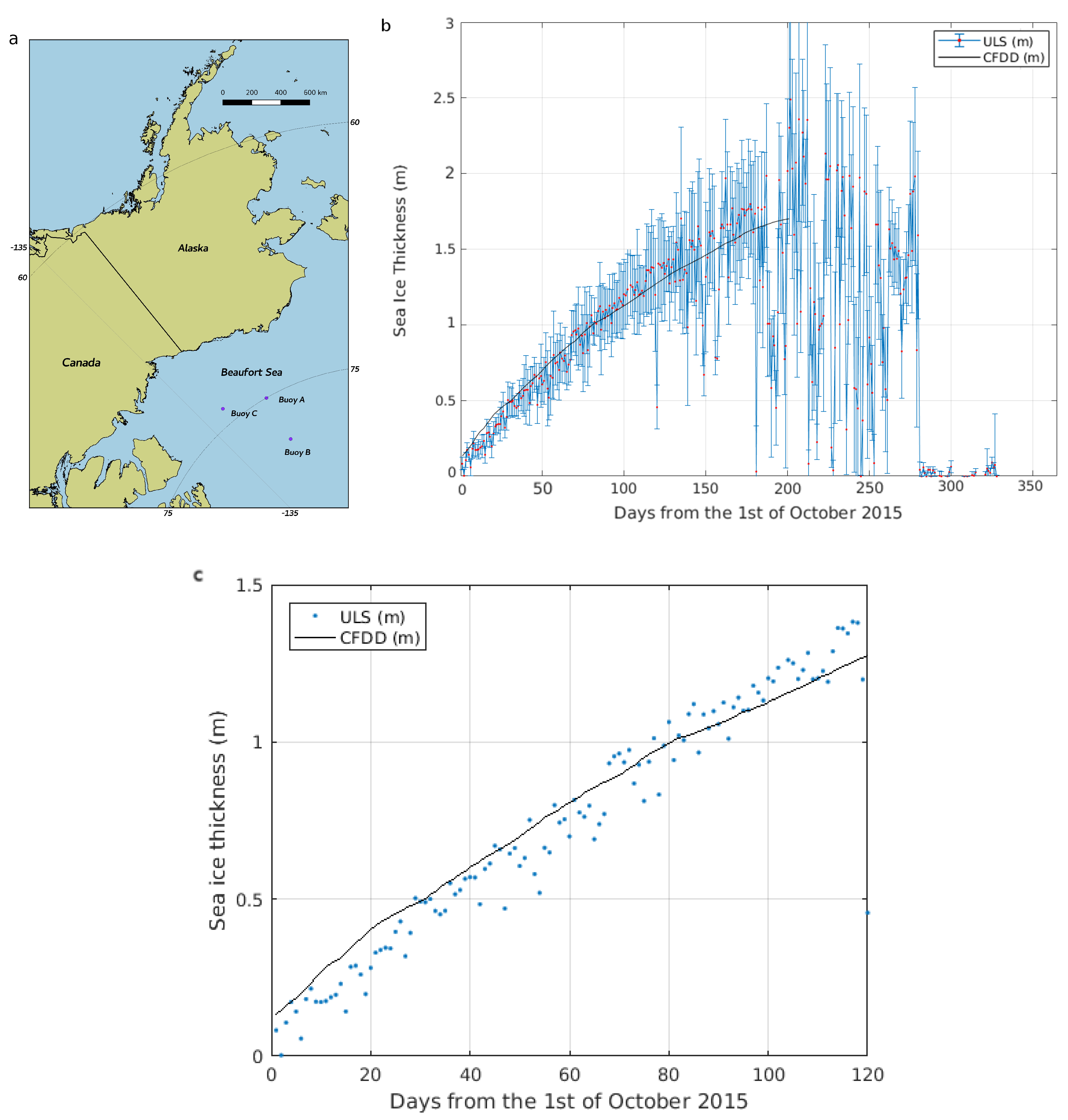
2.3. Moored Upward Looking Sonar

SIT measurements from in-situ moored ULS are available since the early 1990s [24]. The measuring unit from the BGEP consists of several instruments: an Acoustic Doppler Current Profiler (ADCP), an ice-profiling sonar (IPS) with a pendulum and pressure sensors. The ADCP is an echo sounder that measures motion by using the Doppler shift of a target [30]. The IPS measures the distance to the ice-water interfaces. The sonar is made up of an amount of transducers that shape a fine acoustic beam of 2° at −3 dB [24]. This sharp beam permits sampling a target at 50 m distance with a ∼2 m resolution. The pendulum and pressure sensors allow us to estimate the tilt of the beam and the depth of the moored ULS, respectively. Inferring the depth from the pressure implies the knowledge of the atmospheric pressure which must be subtracted (pressure from a nearby weather station often suffices) [24]. The sampling rate is 0.5 Hz, generating files with more than 40,000 samples per day. The uncertainty of the SIT measurement is of 5–10 cm, and depends on a number of factors [24].

Three in-situ moorings located in the Beaufort Sea (see Figure 1) are used in this study. Data collected between 2010 and 2017 during the freeze-up period of the year; i.e., October–January, are analyzed. The total surveyed track length, assuming an ice drift of ∼8 km/day on average, is ∼20,000 km. This constitutes an unprecedented source of information for validation of current PMR thickness retrievals. Thickness is measured in a Eulerian context (i.e., fixed moorings), thus enabling the analysis of ice thickness development during the freeze-up period. This type of retrievals allow a year-round cost-effective acquisition of ice thickness as opposed to helicopter-based campaigns [14].

2.4. Ancillary Data

Sea Ice Concentration (SIC) maps from the database of the Ocean and Sea Ice Satellite Application Facility (OSI SAF) of the European Organisation for the Exploitation of Meteorological Satellites (EUMETSAT) are used in this study. SIC is estimated from TB observations from the Special Sensor Microwave Imager/Sounder (SSM/I and SSMIS) at 19 and 37 GHz which are corrected for atmospheric effects using the European Centre for Medium-Range Weather Forecasts (ECMWF) model output [31].

Sea Ice drift data from the Polar Pathfinder Sea Ice Motion Vectors [32] available at the NASA NSIDC are also used in this analysis, in particular, Version 4, which includes an improved filtering of the SSMI inputs and updates, i.e., input buoy data and input motion vectors. Ice motion estimates are derived from a number of satellite sensors such as the Advanced Very High Resolution Radiometer (AVHRR), the Advanced Microwave Scanning Radiometer—Earth Observing System (AMSR-E), the Scanning Multi-channel Microwave Radiometer (SMMR), SSMI and SSMI/S sensors, the International Arctic Buoy Programme (IABP) and NCEP/NCAR Reanalysis forecasts [32].

Finally, NCEP/NCAR Reanalysis 1 surface air temperatures [33] at 2.5 degrees resolution in latitude and longitude, with a mean absolute error of ∼0.25 and 1.25 degrees Celsius in summer and winter, respectively [34], are used in this analysis. NCEP data together with the empirical Cumulative Freezing Degree Days (CFDD) model are used to calculate SIT [35,36].

$$SIT\left[m\right]=1.33\ast {\left(CFDD{[}^{\circ }C]\right)}^{0.58},$$

(1)

The following procedure is applied in order to obtain SITs from surface temperatures. Sea ice freezing temperature is subtracted from the available NCEP/NCAR surface air temperatures. We apply the modulus function to the resulting temperatures. The resulting value is added from the beginning of the freezing period (i.e., end of September-beginning of October) to the date under consideration. This cumulative quantity is used as an input in Equation (1) to obtain the desired SITs.

3. L-band Passive Radiometer Ice Thickness

Two algorithms for SIT retrievals have been proposed in the literature: one empirical and another one based on the thermodynamic/radiative-transfer model. The empirical methodology was firstly proposed by [11]. It consists of an exponential function that relates the measured intensity or First Stokes parameter (i.e., the average of the horizontally and vertically polarized TBs) with SIT. The intensity is used because of its better quality and signal preservation (e.g., less affected by Faraday rotation) as compared to the co-polarized TBs.

The L-band SIT empirical retrieval is based on Equation (2):

$$\begin{array}{c}\hfill T_{obs}=T_1-(T_1-T_0)exp(-\gamma d)\\ \hfill d\pm \delta d=-\frac{1}{\gamma }ln(\frac{T_1-T_{obs}\pm \delta T_{obs}}{T_1-T_0}),\end{array}$$

(2)

where d is the inverted ice thickness, $\gamma$ the attenuation factor, $T_1$ and $T_0$ the saturated thick ice and the open water signals respectively, and $T_{obs}$ the observed brightness temperature.

This algorithm has been further developed by [13], including a new fitted function describing the Polarization Difference (PD) dependence on SIT. Also the incidence angle used is different: while [12] uses the incidence angle range of 0–40°, [13] uses the observations retrieved at 40°. Additionally, [13] relies on ice growth models for generating the training dataset. More recently, a method that combines the SMOS and SMAP TBs to produce a state-of-the-art SIT product has been developed [21]. The empirically-based product used in this study is produced and supported by the University of Bremen. They currently distribute a version ingesting the SMOS TBs observations. The retrieval is limited to 50 cm ice thickness [13,21]. Allegedly, the SIT error increases with ice thickness and it could amount up to 50% of the retrieval values [21].

The thermodynamic/radiative-transfer model methodology was first developed by the University of Hamburg [12]. The ice thickness is estimated using an iterative approach due to the dependence of SIT on temperature and ice salinity [12]. The ice thickness estimated by [11], which is calculated with average values of $T_{ice}$ and $S_{ice}$ for the Arctic, is used as a first guess in the initial iteration. The temperature of the ice pack is assumed to be the average of the sea water freezing temperature and the surface air temperature from atmospheric reanalysis data [12]. Sea ice salinity, also required by the radiation model, is estimated with the empirical function defined by [37] using the sea surface salinity based on climatology as input. The thickness retrieval convergence is based on the comparison between the observed intensity at nadir (from 0 to 40° incidence angle) and the modeled intensity from an adaptation of the radiation model by [9]. The obtained thickness field is further refined by applying a lognormal distribution [38] that takes into account the effect of subpixel-scale heterogeneity at SMOS resolution [12]. The limits of this type of retrieval are variable depending on the temperature and salinity of the ice pack. It can reach up to 1.5 m under very special conditions, i.e., low temperatures and low salinities, only attainable at closed seas or water masses with large amounts of fresh water supplies (e.g., Baltic Sea) [12]. The SIT uncertainty increases with thickness and it can be larger than the estimated thickness [12].

The presence of snow over sea ice modulates the L-band signature. The wet snow acts as an absorbent at this frequency, thus suppressing the sea ice thickness sensitivity when wet snow is present. This is the reason why the SMOS SIT maps are not produced from mid April to mid October. On the other hand, the dry snow produces a bias in the TB, especially in the H-polarization TB as already stated in [39].

4. Methodology

The ULS data shows its suitability as SIT reference dataset or ground truth when checking its consistency for the continuous sampling of the ice pack during the freeze-up period. The ground truth data acquisition relies on the drifting nature of the sea ice [24]. The ULS thickness reference is re-sampled into the EASE grid for comparison against L-band radiometer thickness products and CFDD SIT based on NCEP/NCAR surface reanalysis data. To produce a suitable ground truth for comparison against satellite measurements, the ULS data are time averaged over consecutive 24-h spans, i.e., the same time resolution of the daily L-band thickness products.

The total amount of measured samples (which equals the number of measured days during the freeze-up period) was ∼2500 which multiplied by the average daily sea ice drift gives a figure of approximately 20,000 km of sampled ice thickness. We imposed a filtering criterion over the time averaged ULS ground truth. The filtering was performed in a two step approach. Firstly, leads were discarded from the statistics whenever their presence in the daily sample was above 5%. Secondly, the daily standard deviation of the ULS dataset with a threshold of 0.2 m was used as a filtering criterion. The latter implied the filtering of approximately $\sim 30\%$ of the ULS measured ice thickness. The filtered ULS ice thickness showed its suitability as ground truth given its accuracy, consistency and continuous record of the ice thickness.

To ensure the statistical representativeness of the derived ground truth, we perform a quality control of the ULS data based on three consistency criteria. First, the ice profile sample (dependent on the amount of ice drift) must be long enough; we imposed a minimum of ∼100 days of sampling which translated into ∼800 km of sampled ice thickness. Second and third, the variability of the SIT profile and SIT field in the perpendicular direction to the profile, respectively, must be low enough; here again, we imposed a threshold of ∼0.2 m in the ice thickness standard deviation. A mean ice drift of ∼7–8 km day−1 for the entire sampling period was estimated on the location of the moorings using both the in-situ ADCP [24] and the NSIDC sea ice velocity record [32]. The variability of the temporally-averaged thickness was calculated with the daily standard deviation of the dataset. Finally, the latter value was used as a proxy for estimating the variability of the ice in the perpendicular direction of the sampled profile.

Figure 1 shows the Buoy C and the CFDD SIT evolution over the freeze-up period in 2015. There is a good match between the ULS thickness data and the CFDD modeled SIT. The temporal evolution of the SIT ground truth shows an increasing standard deviation of the ice thickness daily mean while spring approaches. The thickness values stop increasing at the beginning of spring. As soon as this happens, the ice thickness daily mean begins to change more rapidly. Note also that the SIC increases rapidly at the beginning of the freeze-up period. The former facts indicate that the most suitable time for carrying out a calibration or assessment of L-band ice thickness is precise during the freeze-up period, after the SIC reaches nominal values around 95%, and before the in-situ ice thickness loses its representativeness of satellite resolution scales (i.e., beginning of spring).

We performed the comparison between the daily SIT ground truth and the University of Hamburg (UH) and University of Bremen (UB) SIT products. The UH product provides an uncertainty and a saturation field to inform the users about the quality of the product. As such, the UH SIT data were filtered by using these two parameters following [2]. The filtering was performed using a 1-m uncertainty and a 90% saturation ratio (i.e., the ratio of the estimated thickness to the maximum theoretical retrieval). This filtering procedure reduces the number of ground truth match-ups to approximately one third of its original size, thus triggering the need to extend the validation dataset using model-based SIT data. The comparison between the ground truth and the CFDD SIT (see Equation (1)) shows that the latter is in a first approximation a good estimate of the former as a reference dataset.

The use of CFDD model-based SIT facilitated the extension of the validation. However, this extension was grounded on the homogeneity hypothesis (i.e., the sea ice growth conditions in other regions are considered similar to those found at the buoys’ locations). This hypothesis can only be valid during the freeze-up period when the ice growth is fast and the impact of the ice drift is lower on the CFDD modeled ice thickness.

The scatter plot between the ULS-derived ground truth collected over 7 years during the freeze-up periods (from 2010 to 2016) and the co-located CFDD SIT is shown in Figure 2. The scatter indicates that CFDD SIT is a good proxy of the ground truth having only small deviations from the identity line, the regression factor is ∼0.99 ± 0.01 at 95% confidence level. Indeed, the CFDD SIT represents quite well ice thickness up to 0.3 m. For larger SIT values, a slight overestimation of the CFDD data is noticeable. We attribute this overestimation to the inability of the model to represent events of strong ice drift that inhibit ice growth for several days. This good correlation between both datasets does not hold for the late winter-early spring months (see Figure 1). Therefore, we only use the CFDD SIT as proxy of the ULS ground truth during the freezing season (i.e., from October to January), and in regions with thin first-year sea ice.

5. Results and Discussion

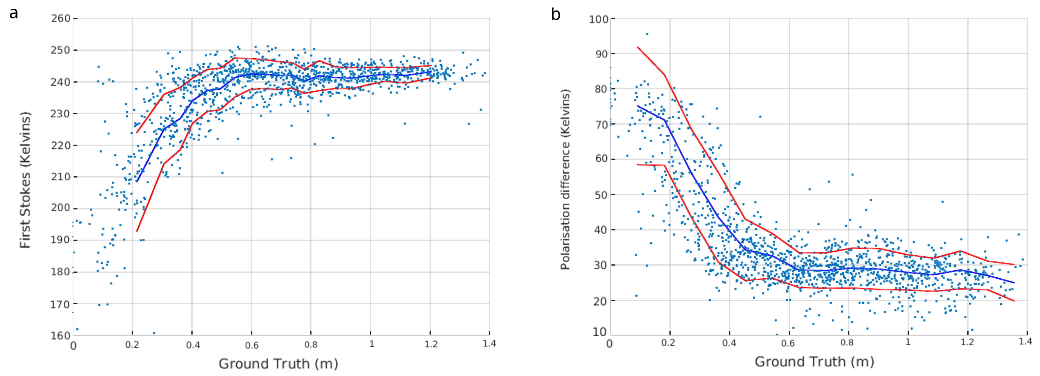
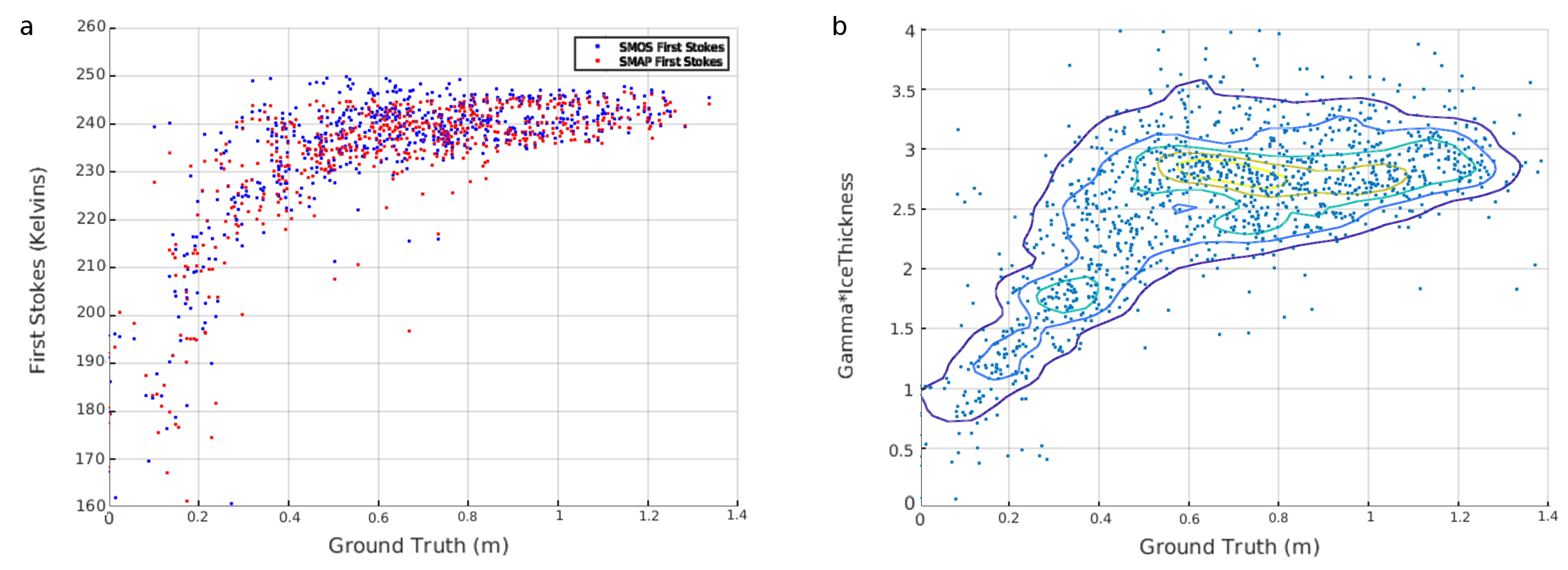
5.1. L-band Response to SIT

Using the ground truth as described in the previous section allows establishing the relation between SMOS and SMAP L-band First Stokes parameter, the PD and the SIT parameter. Figure 3 and Figure 4 show some L-band parameters as functions of the ground truth, which is filtered with a 95% SIC threshold in all cases. It should be noticed that recent efforts for characterizing the L-band response to ice thickness were hindered by the distribution and characteristics of the ground truth used [2,14,22]. On the one hand, the spatial distribution of the ground truth is limited to those regions sampled by ships. On the other hand, campaigns are normally carried out at the end of winter or in spring, therefore a thickness seasonal bias can be expected [14,22]. The author in [2] uses the Ocean ReAnalysis System 5 (ORAS5) modeled ice thickness for their comparison against SMOS SIT. They notice an overestimation of the ORAS5 with respect to SMOS SIT. This is attributed to the simplified representation of thin ice by the model (see [2] for further details).

Figure 3 displays the relationship between the First Stokes and PD parameters and the daily ULS ground truth. The First Stokes parameter shows a large dispersion for thin ice which decreases with increasing ice thickness. Such a decrease in dispersion reveals a saturation of the response of TB to large SIT values (i.e., above 0.6 m). The signal saturates at a value of ∼240 Kelvins. The standard deviation of the TB at large SIT values is in fact an estimation of the radiometric error of the observation system, because at such SIT values, the signal no longer responds to the geophysical parameters and the variability can be mainly attributed to the radiometric noise.

A theoretical relationship between TB and ice thickness based in the incoherent Burke model can be found in [10] and [12]. We note here that larger dispersion is seen for very thin ice while other comparisons between these parameters show that the largest dispersion is found at around 20 cm ice thickness [12,13]. Probably, several physical mechanisms not considered in the theoretical model can be affecting the TB response to thin ice, such as the impact of ice surface temperature and ice surface roughness variations, among others.

The relationship between SMOS PD and the ground truth can be found in Figure 3b. The PD presents a constant but larger standard deviation (with respect to the case of the First Stokes parameter) for ice thinner than 0.6 m, and for thicker ice the PD saturates at a value slightly below ∼30 Kelvins. The PD intersects with the ordinate axis at ∼70–80 Kelvins. In contrast, [13] indicates an intersection at around 50 Kelvins. We attribute this difference either to a wrongly classified thickness with the CFDD model by [13] or to the inclusion of pixels with different SICs in their analysis.

In order to confirm the L-band response to SIT, as shown by SMOS data (see Figure 3), we perform the same analysis but with SMAP TB. The comparison between SMOS and SMAP TB responses to ice thickness is shown in Figure 4a. The L-band signal response from both sensors presents very similar patterns, including larger dispersion for thin ice and saturation for thick ice. Nonetheless, SMAP TBs are slightly lower for thick ice than those of SMAP, something that can be a consequence of SMOS residual biases [41].

We estimated the standard deviation of the ice thickness retrieval by propagating the TB error to the SIT according to Equation (2). Surprisingly, the standard deviation of ice thickness increases with increasing thickness, as opposed to what happens with the TB. This is due to the formulae used in the thickness retrieval and the larger sensitivity of TB to SIT for thin ice.

The limit of validity of the empirical retrieval is located around the 0.5 m SIT [11,13]. In order to further constrain this limit, we analyzed the factor within the exponential term in Equation (2), $\gamma d$, which corresponds to a normalized thickness. The scatter plot of Figure 4b evidences the relation between ground truth and the normalized thickness. As expected, we see an almost linear relation for ice thinner than 0.6 m. Besides, the dispersion of the parameter increases with ice thickness and finally, for thicker ice, the sensitivity of TB to SIT is completely lost. The scatter points in that region are distributed around a horizontal line (hence, the attenuation factor $\gamma$ is meaningless in that region). Obviously, this limitation applies only to the pure empirical retrieval. The thickness retrieval can be extended to thicker ice using a radiative transfer model and assuming a lognormal distribution [12]. However, this approach can be sensitive to the auxiliary fields used, such as SIC, temperature and salinity, whose uncertainties can be difficult to quantify [2].

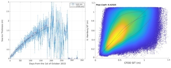
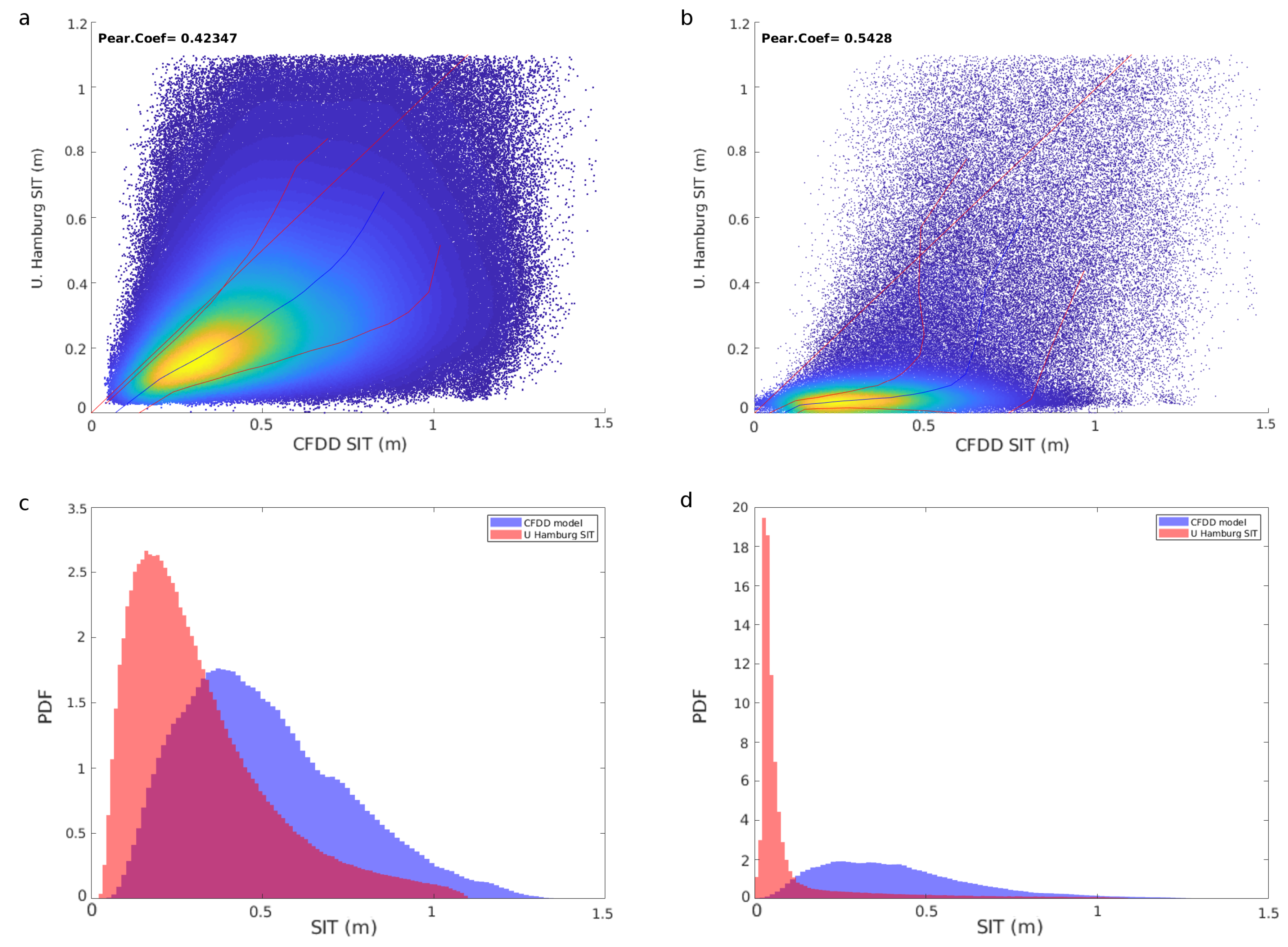
5.2. Assessment of UH SIT

The direct comparison between the UH ice thickness and the ground truth reveals that the product underestimates thin sea ice and overestimates thickness larger than 0.3 m (see Figure 5a). This underestimation for thin ice and its relationship with SIC has been widely reported in the literature [2,12]. Considering that CFDD is already overestimating the ULS ground truth for thick ice (see Figure 2), a larger thickness overestimation of the UH product with respect to ULS is expected for thick ice (see Figure 5b and Section 4). The ice thickness standard deviation increases with thickness (see Figure 5b). The observed decrease in the standard deviation for large thickness is due to the decrease of the scatter region analyzed in the calculation.

The CFDD thickness and the ULS scatter plots against the UH SIT reveal with their similarity that the proposed homogeneity hypothesis works fine during the freeze-up periods. This situation provides a solid ground for extending the ULS ground truth with the CFDD ice thickness.

The Probability Density Functions (PDFs) for the freeze-up period for SIC over 90% reveals that the modes values are of similar value for UH and CFDD SITs (see Figure 5). Moreover, the shape of both PDFs are similar. However, UH PDF shows a smoother shape, with gentle slopes and a larger amount of occurrences for thickness above 0.5 m (see Figure 5d). Interestingly, a different PDF is observed for UH SIT during October, at the beginning of the freeze-up period (see Figure 5c). In this case, the modes of both distributions are coincidental as was the case for the whole-winter period. However, the shapes of the distributions are markedly different, even when considering that the CFDD model SIT is around observable values for the SMOS-based L-band SIT retrieval valid range (i.e., from 0.1 to 0.6 m), indicating poor-quality SMOS SIT retrievals, even at these favorable conditions (i.e., for high SIC conditions). A possible explanation for this change on the distribution shape could be the application of the lognormal distribution to the largest thickness values [12]. This change in the shape of the distribution is no longer visible for lower SICs.

The analysis of the distributions with lower SIC values (see Figure 6) indicates that the UH product bias increases with decreasing SIC. Furthermore, the UH SIT distribution is more peaky with decreasing SIC. The increasing negative bias of the product with decreasing SIC has already been reported by [12]. The peaky behavior of the distribution might reveal that the retrieval algorithm is saturated for low SIC values. On the other hand, the thickness distribution for SICs between 70% and 90%, while having a bias, presents a very similar shape to that of the CFDD SIT (see Figure 6c). The latter facilitates a possible readjustment of the product using a simple shift. The distribution of SIT in cases with lower SICs has both a large bias and peaks at lower SIT values (see Figure 6d). In this case, a readjustment would require both a shift and a rescaling provided that the ice thickness signal is still present in the measured TB and is not contaminated by the ocean signal.

The UH SIT product well reproduces the distribution for the whole freeze-up period for high SIC values (see Figure 5d). However, we recognize the inability of the UH algorithm to represent the real distribution of SITs for high SIC (i.e., above 90%) during specific periods of the year (e.g., October). However, this distribution facilitate that UH product better represents the end of winter fully developed ice for high SICs. During the same period of the year, when lower SICs are considered, UH product departs from CFDD ice thickness. Moreover, we see both the increasing underestimation and kurtosis (peakiness) of the distributions with decreasing SICs (see Figure 6). The satellite sampling which permits a daily coverage for the whole Arctic region [15] contrasts with the limitations of the thickness retrieval for specific periods of the year (see Figure 5c). The inability of the UH product to capture the temporal trend of the ice thickness at high SICs is a significant concern since the satellite temporal resolution is left unexploited (i.e., the retrievals do not properly reflect the real ice thickness distribution for a given time). The latter leaves the door open for future improvements with a temporally enhanced thickness retrieval.

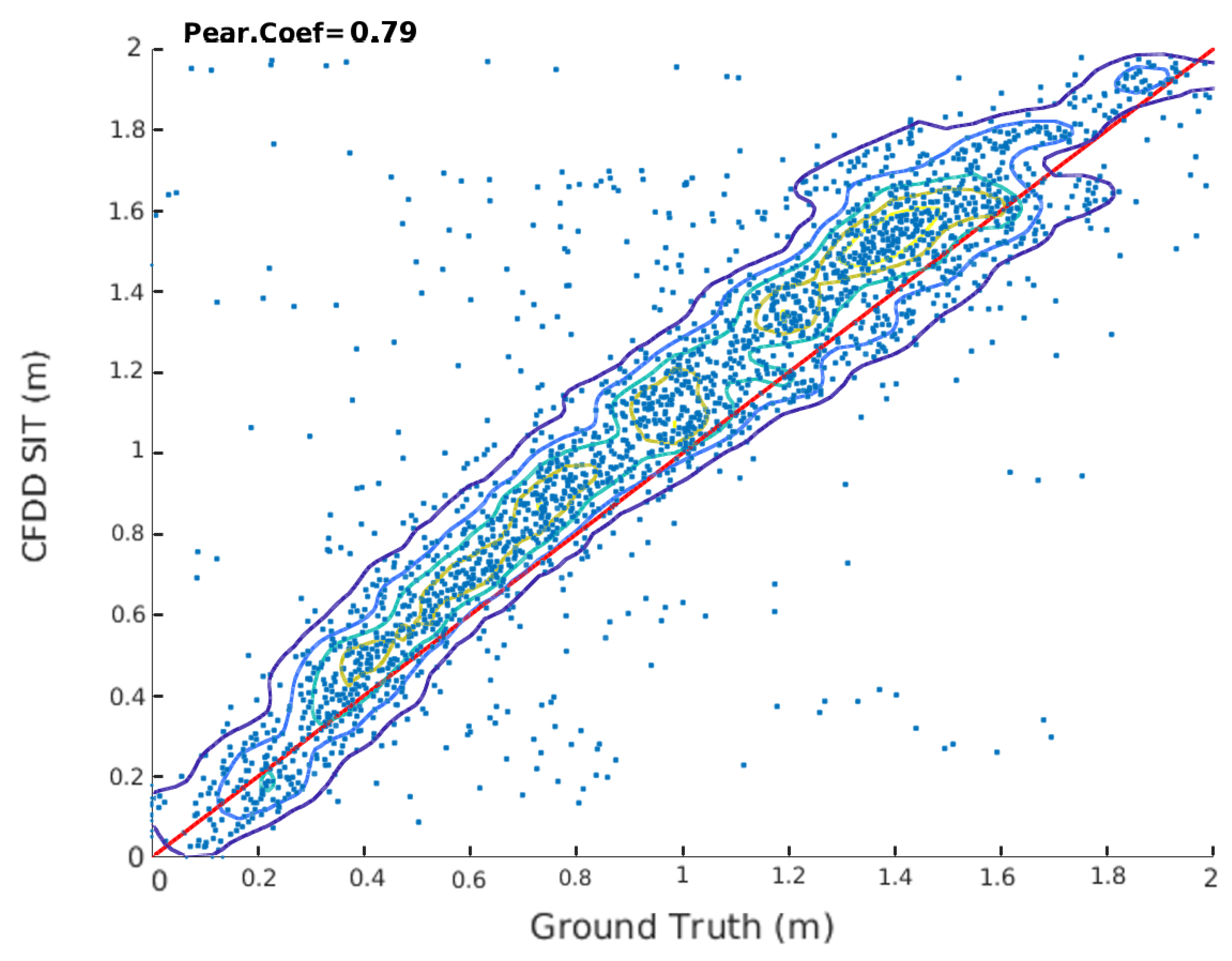
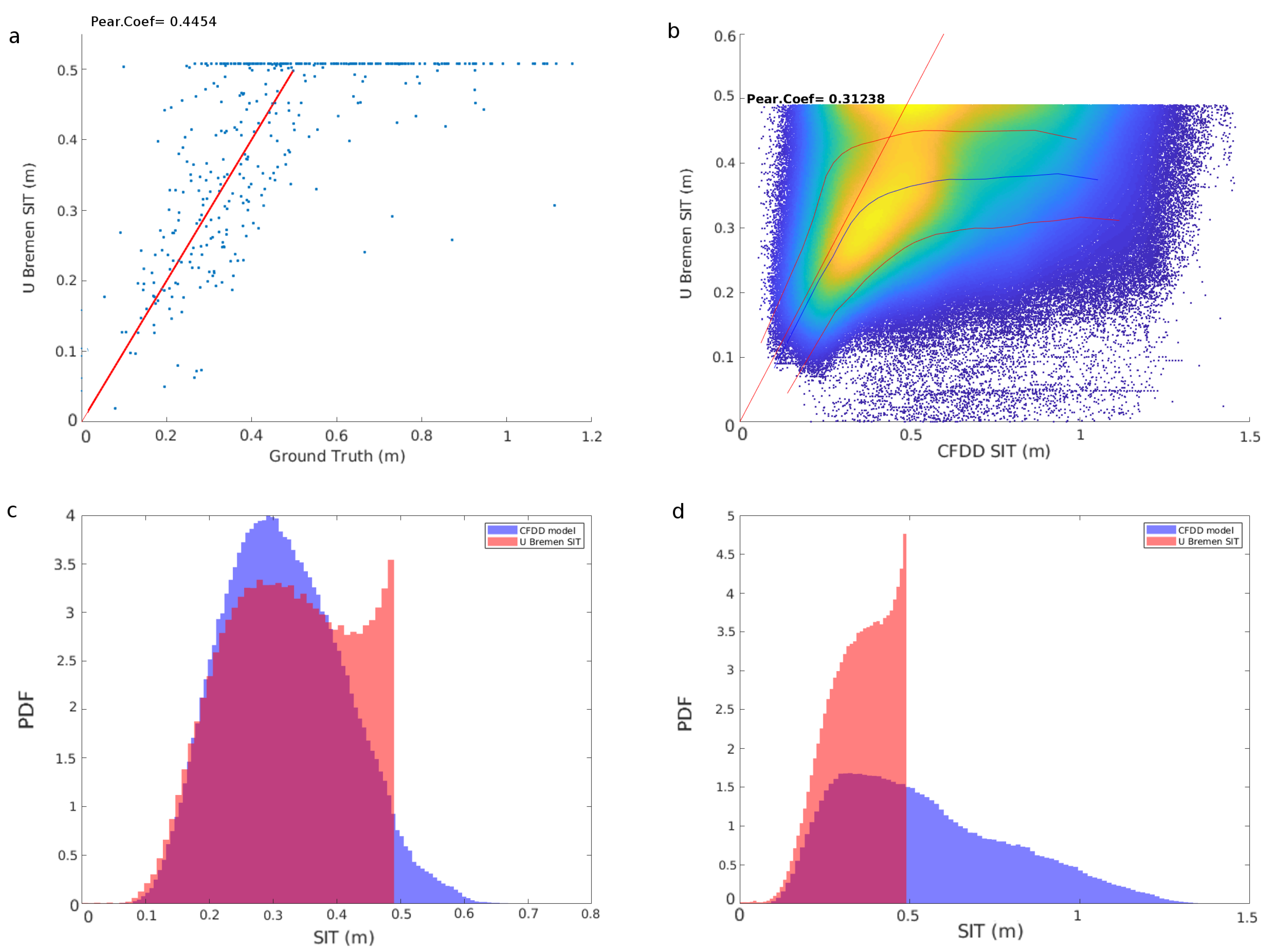
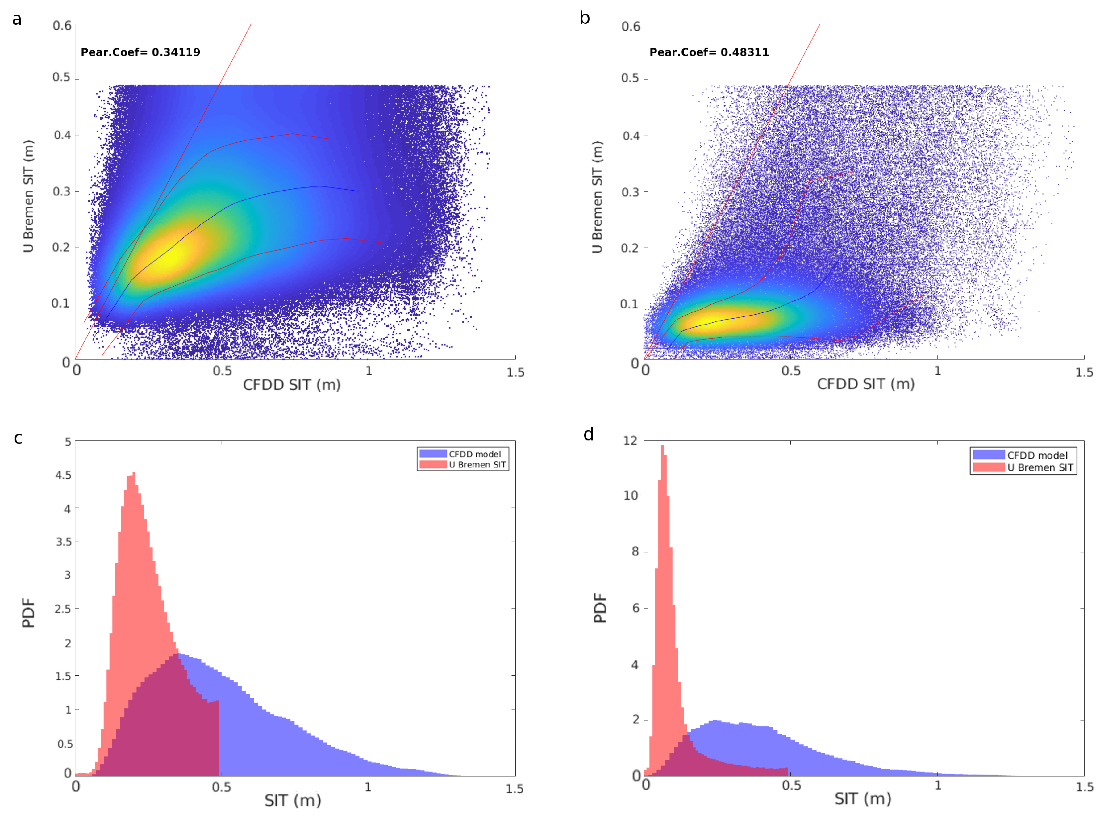
5.3. Assessment of UB SIT

The following comparisons were carried out filtering the UB SIT based on the UH restrictions of saturation and uncertainty. The methodology makes the comparison between products and ground truth more consistent and reliable, because we are comparing the same datasets. The analyzed UB SIT cells are sometimes saturated and sometimes fall within the observable thickness range, when saturated they are also filtered (i.e., above 0.5 m). The scatter plot between the buoy ULS thickness and the UB SIT indicates that the UB product underestimates SIT for the whole freeze-up period (see Figure 7b). The UB thickness shows a large amount of occurrences near the saturation limit. We interpret this as an indication that the algorithm is trying to represent in the range of half a meter CFDD thickness values that are clearly over their own retrieval limit (see Figure 7d). We also observe that ice thickness standard deviation increases with thickness (see Figure 7b). In contrast with the UH product, only a slight SIT underestimation is present in the UB product for thickness below 0.4 m, indicating a relatively higher accuracy of the latter within the mentioned thickness range.

Here again, as what happened with the UH SIT, the CFDD thickness and the ULS scatter plots’ similarity supports the proposed homogeneity hypothesis. Therefore, we have further support for using the CFDD SIT as an Arctic-wide proxy of SIT ground truth.

Indeed, the UB SIT marginal distribution resembles that of CFDD, for the month of October and SIC above 90% (see Figure 7c). The CFDD thickness values are within the observable L-band thickness range (0–0.5 m), and therefore they are expected to be resolved as they do (as opposed to UH product, see Section 5.2). The good fit comes as no surprise since the UB product is based on the CFDD model and the NCEP/NCAR surface reanalysis auxiliary data [13]. The observed good fit during October is no longer seen for later periods (i.e., from November to January) when UB is not able to resolve CFDD thickness values lying over the retrieval limit (see Figure 7d).

The UB SIT behavior when considering decreasing SIC values is similar to that of the UH product, i.e., an increasing bias and a more peaky distribution on the thinner thickness range (see Figure 8). The distributions reveal that the UB product is wrongly classifying thickness above 0.5 m, by setting them to a fixed value of 0.5 m. The wrongly classified CFDD thickness, calculated after filtering the saturated UB SIT, amount to 50% of the total (this percentage is calculated for the whole freeze-up period, considering values of SIC above 90%). The UB thickness products caps the retrievals at 0.5 m [13] taking into account the limits of the empirical retrieval. By doing so, they are indirectly forcing an artificial saturation visible in all comparisons. On the positive side, we see the related bias of the acquisition for lower SICs, a similar behavior seen for both UB (see Figure 8c,d) and UH (Figure 6a,d) SIT, although the former shows a slightly smaller bias (with respect to ground truth) than the latter.

5.4. Applicability of the L-band SIT Retrieval Methodology

Assuming that L-band technology is only sensitive to thin ice conditions, the coverage of potentially useful L-band SIT retrievals is analyzed in this section.

Figure 9a shows the sea ice extent for all sea ice cells (i.e., SIC above 15%) and for those cells with specific ice conditions (red curve) and retrievable thin ice (green curve), while Figure 9b shows the latter as percentages with respect to the total sea ice extent. Figure 9b shows that relative percentages of retrievable thickness are highest at the beginning of the freeze-up period (i.e., October–November). Furthermore, when considering the optimal retrievable thickness range (i.e., below 0.5 m), this part of the year has also the largest share of observable ice thickness. Interestingly, as the freezing period progresses, the respective shares of observable thickness drop, but between them, the optimal retrievable thickness presents a further drop below 5% of the total sea ice extent (see Figure 9b).

It is also relevant to stress the limited temporal coverage of the L-band based SIT products, mainly valid during the freeze-up period and in regions of high SIC values (e.g., during October–November in the Northern Hemisphere). These optimally observable regions are typically located outside the multi-year ice holding half-ringed shape (i.e., a partial ring spanning from the northern coasts of Canada and Russia); eventually, this ring-shaped structure closes when reaching the Bering Strait. These regions shrink in size as the winter progresses (see Figure 9b), thus leading to poor-quality SIT retrievals due to the relatively low spatial resolution of the SMOS satellite. Therefore, optimal retrievable values are expected to be mainly located in these temporally and spatially-varying regions.

6. Conclusions

We have characterized the brightness temperature response to SIT using the processed upward looking sonar ground truth during the freeze-up period between October and January from BGEP from WHOI. TB shows a larger dispersion for thin sea ice, increases with SIT and saturates for ice thicker than 0.6 m at approximately 240 Kelvins where the effect of SMOS radiometric uncertainty (radiometric noise) is visible. PD intersects the ordinates axis between 70 and 80 Kelvins and saturates for ice thicker than 0.6 m at approximately 30 Kelvins. The observed dispersion of the TB propagates into the ice thickness estimation with a standard deviation that increases with ice thickness. The analysis of the attenuation parameter of the empirical retrieval reveals the lack of response of the TB to SIT thicker than 0.6 m.

The year-round, cost-effective, accurate record of ULS SIT and the lack of validation data stresses the strong need of deploying and maintaining more measuring units at appropriate locations of the Arctic Ocean. This approach would probably improve the quality and usefulness of validation data with respect to current costly ship-based campaigns performed so far for gathering SIT ground truth with EM [14,22,23], that are also very limited as they can only be done during late winter–early spring months due to the need of helicopter which entails measuring a fully developed ice pack therefore skewing the reference dataset.

The detailed comparison between CFDD-model SIT and ULS ground truth evidenced their strong correlation during the freeze-up period. We have taken advantage of this correlation to use the estimated CFDD SIT as a reference dataset during the freeze-up periods. Furthermore, we saw the similarity of the scatter plots between CFDD and ULS against UH and UB SIT products revealing again the strength of the proposed homogeneity hypothesis. The extension of the ground truth with the model-based thickness allowed characterizing the L-band ice thickness products in different scenarios. The analysis showed that L-band SIT present a clear dependency on SIC while this parameter is not considered in current SIT estimations [12,13].

The comparison between the CFDD SIT and UH SIT product at 90% SIC shows that their modes are coincident during the whole freeze-up period and also partially at other periods. UH SIT slightly underestimates for thicknesses below 0.3 and overestimates for thicker ice. However, the shapes of the PDFs of CFDD SIT and UH SIT, while being similar for the whole winter, becomes notoriously different at specific months. On the other hand, as the freezing period advances UH SIT mode corresponds to the CFDD SIT mode. This change in the shape of the distribution is probably needed to accommodate thickness values outside the L-band observational range and probably relates to the lognormal distribution [12]. As SIC is gradually lowered in the comparison, there is a trend of increasing bias and the UH distribution becomes concentrated at low thicknesses. The shape of both distributions are very similar when the SIC is between 70% and 90%, an encouraging starting point for improving the already visible bias at this concentration range.

The comparison between the CFDD SIT and UB SIT product at 90% SIC indicates that UB SIT fits the ground truth very closely for thickness below 0.4 m. For thicker ice, UB SIT has a tendency to give a saturated response. This saturation stems from the fact that many CFDD thickness values (around 50%) over half a meter are wrongly classified by UB. However, the thickness distribution for October presents a shape very close to that of CFDD distribution. The latter comes as no surprise since [13] product is trained using the CFDD SIT model as a reference. Nonetheless, as the freeze-up period continues, the CFDD SIT distribution displaces to larger thickness outside the empirical retrieval observable range. In these cases UB SIT saturation is more pronounced. As SIC is decreased in the comparison, UB SIT presents an increasing negative bias and its distribution peaks at lower thickness (following exactly the same behavior as the UH product).

The former analysis permits us to understand the current limitations of SMOS-based ice thickness products. These limitations are not only related to the retrieval methodology but also to the geographical extent where L-band based SIT is applicable. There are specific periods of the year when optimal retrieval conditions are only reached for 5% or less of the whole sea ice Arctic coverage. This scarce coverage challenges the consideration of L-band-based SIT as an Arctic wide product. Regarding the methodological limitations, we indicate a minimum of ∼90% SIC for a successful thickness retrieval during the freeze-up period when the ice pack thickness remains below half a meter.

The observed limitations of the retrieval methodologies strongly suggest future lines of improvement. Considering the daily temporal resolution of the satellites, a temporally enhanced SIT retrieval would be a step ahead. This temporal adjustment would allow to present a temporally consistent SIT product with no variations in its behavior during the winter. The second line of improvement stems from the need of considering SIC as a required variable for SIT retrieval. This would permit adjusting the thickness inversion depending on the considered SIC. If the latter is not possible, indicating at least the ice concentration for the specific retrieved values as a quality flag is an absolute must. This would give the user fundamental information about the quality of the estimated ice thickness.

References

1. Ivanova, N.; Pedersen, L.T.; Tonboe, R.T.; Kern, S.; Heygster, G.; Lavergne, T.; Sørensen, A.; Saldo, R.; Dybkjær, G.; Brucker, L.; et al. Inter-comparison and evaluation of sea ice algorithms: Towards further identification of challenges and optimal approach using passive microwave observations. Cryosphere 2015, 9, 1797–1817. [Google Scholar] [CrossRef] [Green Version]
2. Tietsche, S.; Alonso-Balmaseda, M.; Rosnay, P.; Zuo, H.; Tian-Kunze, X.; Kaleschke, L. Thin Arctic sea ice in L-band observations and an ocean reanalysis. Cryosphere 2018, 12, 2051–2072. [Google Scholar] [CrossRef] [Green Version]
3. Maykut, G.A. Energy exchange over young sea ice in the central Arctic. J. Geophys. Res. 1978, 83, 3646. [Google Scholar] [CrossRef]
4. Kwok, R.; Cunningham, G.F.; Zwally, H.J.; Yi, D. Ice, Cloud, and land Elevation Satellite (ICESat) over Arctic sea ice: Retrieval of freeboard. J. Geophys. Res. 2007, 112. [Google Scholar] [CrossRef] [Green Version]
5. Kwok, R.; Cunningham, G.F. ICESat over Arctic sea ice: Estimation of snow depth and ice thickness. J. Geophys. Res. 2008, 113. [Google Scholar] [CrossRef]
6. Zwally, H.J.; Yi, D.; Kwok, R.; Zhao, Y. ICESat measurements of sea ice freeboard and estimates of sea ice thickness in the Weddell Sea. J. Geophys. Res. 2008, 113. [Google Scholar] [CrossRef] [Green Version]
7. Laxon, S.W.; Giles, K.A.; Ridout, A.L.; Wingham, D.J.; Willatt, R.; Cullen, R.; Kwok, R.; Schweiger, A.; Zhang, J.; Haas, C.; et al. CryoSat-2 estimates of Arctic sea ice thickness and volume. Geophys. Res. Lett. 2013, 40, 732–737. [Google Scholar] [CrossRef] [Green Version]
8. Mäkynen, M.; Cheng, B.; Similä, M. On the accuracy of thin-ice thickness retrieval using MODIS thermal imagery over Arctic first-year ice. Ann. Glaciol. 2013, 54, 87–96. [Google Scholar] [CrossRef] [Green Version]
9. Menashi, J.D.; Germain, K.M.S.; Swift, C.T.; Comiso, J.C.; Lohanick, A.W. Low-frequency passive-microwave observations of sea ice in the Weddell Sea. J. Geophys. Res. 1993, 98, 22569. [Google Scholar] [CrossRef]
10. Kaleschke, L.; Maaß, N.; Haas, C.; Hendricks, S.; Heygster, G.; Tonboe, R.T. A sea-ice thickness retrieval model for 1.4 GHz radiometry and application to airborne measurements over low salinity sea-ice. Cryosphere 2010, 4, 583–592. [Google Scholar] [CrossRef] [Green Version]
11. Kaleschke, L.; Tian-Kunze, X.; Maaß, N.; Mäkynen, M.; Drusch, M. Sea ice thickness retrieval from SMOS brightness temperatures during the Arctic freeze-up period. Geophys. Res. Lett. 2012, 39, L05501. [Google Scholar] [CrossRef]
12. Tian-Kunze, X.; Kaleschke, L.; Maaß, N.; Mäkynen, M.; Serra, N.; Drusch, M.; Krumpen, T. SMOS-derived thin sea ice thickness: Algorithm baseline, product specifications and initial verification. Cryosphere 2014, 8, 997–1018. [Google Scholar] [CrossRef] [Green Version]
13. Huntemann, M.; Heygster, G.; Kaleschke, L.; Krumpen, T.; Mäkynen, M.; Drusch, M. Empirical sea ice thickness retrieval during the freeze-up period from SMOS high incident angle observations. Cryosphere 2014, 8, 439–451. [Google Scholar] [CrossRef] [Green Version]
14. Kaleschke, L.; Tian-Kunze, X.; Maaß, N.; Beitsch, A.; Wernecke, A.; Miernecki, M.; Müller, G.; Fock, B.H.; Gierisch, A.M.; Schlünzen, K.H.; et al. SMOS sea ice product: Operational application and validation in the Barents Sea marginal ice zone. Remote Sens. Environ. 2016, 180, 264–273. [Google Scholar] [CrossRef]
15. Kerr, Y.; Waldteufel, P.; Wigneron, J.P.; Martinuzzi, J.; Font, J.; Berger, M. Soil moisture retrieval from space: The Soil Moisture and Ocean Salinity (SMOS) mission. IEEE Trans. Geosci. Remote Sens. 2001, 39, 1729–1735. [Google Scholar] [CrossRef]
16. Entekhabi, D.; Njoku, E.G.; O’Neill, P.E.; Kellogg, K.H.; Crow, W.T.; Edelstein, W.N.; Entin, J.K.; Goodman, S.D.; Jackson, T.J.; Johnson, J.; et al. The Soil Moisture Active Passive (SMAP) Mission. Proc. IEEE 2010, 98, 704–716. [Google Scholar] [CrossRef]
17. Zine, S.; Boutin, J.; Font, J.; Reul, N.; Waldteufel, P.; Gabarro, C.; Tenerelli, J.; Petitcolin, F.; Vergely, J.L.; Talone, M.; et al. Overview of the SMOS Sea Surface Salinity Prototype Processor. IEEE Trans. Geosci. Remote Sens. 2008, 46, 621–645. [Google Scholar] [CrossRef]
18. Font, J.; Camps, A.; Borges, A.; Martín-Neira, M.; Boutin, J.; Reul, N.; Kerr, Y.H.; Hahne, A.; Mecklenburg, S. SMOS: The Challenging Sea Surface Salinity Measurement From Space. Proc. IEEE 2010, 98, 649–665. [Google Scholar] [CrossRef] [Green Version]
19. O’Neill, P.; Chan, S.; Njoku, E.; Jackson, T.; Bindlish, R. SMAP L3 Radiometer Global Daily 36 km EASE-Grid Soil Moisture. Version 2016, 4, R14010. [Google Scholar] [CrossRef]
20. Mecklenburg, S.; Drusch, M.; Kaleschke, L.; Rodriguez-Fernandez, N.; Reul, N.; Kerr, Y.; Font, J.; Martin-Neira, M.; Oliva, R.; Daganzo-Eusebio, E.; et al. ESA’s Soil Moisture and Ocean Salinity mission: From science to operational applications. Remote Sens. Environ. 2016, 180, 3–18. [Google Scholar] [CrossRef]
21. Paţilea, C.; Heygster, G.; Huntemann, M.; Spreen, G. Combined SMAP–SMOS thin sea ice thickness retrieval. Cryosphere 2019, 13, 675–691. [Google Scholar] [CrossRef] [Green Version]
22. Maaß, N.; Kaleschke, L.; Tian–kunze, X.; Mäkynen, M.; Drusch, M.; Krumpen, T.; Hendricks, S.; Lensu, M.; Haapala, J.; Haas, C. Validation of SMOS sea ice thickness retrieval in the northern Baltic Sea. Tellus A Dyn. Meteorol. Oceanogr. 2015, 67, 24617. [Google Scholar] [CrossRef]
23. Haas, C.; Lobach, J.; Hendricks, S.; Rabenstein, L.; Pfaffling, A. Helicopter-borne measurements of sea ice thickness, using a small and lightweight, digital EM system. J. Appl. Geophys. 2009, 67, 234–241. [Google Scholar] [CrossRef] [Green Version]
24. Melling, H.; Johnston, P.H.; Riedel, D.A. Measurements of the Underside Topography of Sea Ice by Moored Subsea Sonar. J. Atmos. Ocean. Technol. 1995, 12, 589–602. [Google Scholar] [CrossRef]
25. Gabarro, C.; Turiel, A.; Elosegui, P.; Pla-Resina, J.A.; Portabella, M. New methodology to estimate Arctic sea ice concentration from SMOS combining brightness temperature differences in a maximum-likelihood estimator. Cryosphere 2017, 11, 1987–2002. [Google Scholar] [CrossRef] [Green Version]
26. Corbella, I.; Torres, F.; Duffo, N.; González-Gambau, V.; Pablos, M.; Duran, I.; Martín-Neira, M. MIRAS Calibration and Performance: Results From the SMOS In-Orbit Commissioning Phase. IEEE Trans. Geosci. Remote Sens. 2011, 49, 3147–3155. [Google Scholar] [CrossRef]
27. Camps, A.; Vall-llossera, M.; Duffo, N.; Torres, F.; Corbella, I. Performance of sea surface salinity and soil moisture retrieval algorithms with different auxiliary datasets in 2-D L-band aperture synthesis interferometric radiometers. IEEE Trans. Geosci. Remote Sens. 2005, 43, 1189–1200. [Google Scholar] [CrossRef]
28. Chan, S.K.; Bindlish, R.; O’Neill, P.E.; Njoku, E.; Jackson, T.; Colliander, A.; Chen, F.; Burgin, M.; Dunbar, S.; Piepmeier, J.; et al. Assessment of the SMAP Passive Soil Moisture Product. IEEE Trans. Geosci. Remote Sens. 2016, 54, 4994–5007. [Google Scholar] [CrossRef]
29. Lannoy, G.J.M.D.; Reichle, R.H.; Peng, J.; Kerr, Y.; Castro, R.; Kim, E.J.; Liu, Q. Converting Between SMOS and SMAP Level-1 Brightness Temperature Observations Over Nonfrozen Land. IEEE Geosci. Remote Sens. Lett. 2015, 12, 1908–1912. [Google Scholar] [CrossRef]
30. Brumley, B.; Cabrera, R.; Deines, K.; Terray, E. Performance of a broad-band acoustic Doppler current profiler. IEEE J. Ocean. Eng. 1991, 16, 402–407. [Google Scholar] [CrossRef]
31. Tonboe, R.; Lavelle, J.; Pfeiffer, R.H.; Howe, E. Product User Manual for OSI SAF Global Sea Ice Concentration; OSI-401-b & EUMETSAT; Danish Meteorological Institute: Copenhagen, Denmark, 2017. [Google Scholar]
32. Tschudi, M. Polar Pathfinder Daily 25 km EASE-Grid Sea Ice Motion Vectors; NASA National Snow and Ice Data Center Distributed Active Archive Center: Boulder, CO, USA, 2019. [Google Scholar] [CrossRef]
33. Kalnay, E.; Kanamitsu, M.; Kistler, R.; Collins, W.; Deaven, D.; Gandin, L.; Iredell, M.; Saha, S.; White, G.; Woollen, J.; et al. The NCEP/NCAR 40-Year Reanalysis Project. Bull. Am. Meteorol. Soc. 1996, 77, 437–472. [Google Scholar] [CrossRef] [Green Version]
34. Mooney, P.A.; Mulligan, F.J.; Fealy, R. Comparison of ERA-40, ERA-Interim and NCEP/NCAR reanalysis data with observed surface air temperatures over Ireland. Int. J. Climatol. 2011, 31, 545–557. [Google Scholar] [CrossRef] [Green Version]
35. Bilello, M.A. Formation, Growth, and Decay of Sea-Ice in the Canadian Arctic Archipelago. ARCTIC 1961, 14. [Google Scholar] [CrossRef]
36. Weeks, W.F. On Sea Ice; University of Alaska Press: College, AK, USA, 2010. [Google Scholar]
37. Ryvlin, A.I. Method of forecasting flexural strength of an ice cover. Probl. Arct. Antarct. 1974, 45, 79–86. [Google Scholar]
38. Key, J.; McLaren, A.S. Fractal nature of the sea ice draft profile. Geophys. Res. Lett. 1991, 18, 1437–1440. [Google Scholar] [CrossRef]
39. Maaß, N.; Kaleschke, L.; Tian-Kunze, X.; Drusch, M. Snow thickness retrieval over thick Arctic sea ice using SMOS satellite data. Cryosphere 2013, 7, 1971–1989. [Google Scholar] [CrossRef] [Green Version]
40. Wessel, P.; Smith, W.H.F. A global, self-consistent, hierarchical, high-resolution shoreline database. J. Geophys. Res. Solid Earth 1996, 101, 8741–8743. [Google Scholar] [CrossRef] [Green Version]
41. Schmitt, A.; Kaleschke, L. A Consistent Combination of Brightness Temperatures from SMOS and SMAP over Polar Oceans for Sea Ice Applications. Remote Sens. 2018, 10, 553. [Google Scholar] [CrossRef] [Green Version]
Figure 1. (a) Location of Woods Hole Oceanographic Institution (WHOI) buoys in the Beaufort Sea. The map uses the Arctic Polar Stereographic projection (EPSG: 3995) [40]. (b) Temporal evolution of the ice thickness measured by Buoy C (red dots) and modeled by Cumulative Freezing Degree Days (CFDD) (black line) over the freeze-up period in 2015. (c) Comparison between the modeled CFDD and Upward Looking Sonar (ULS) ground truth gathered during the first three months of the freeze-up period.
Remotesensing 12 00650 g001
Figure 2. Comparison of the modeled CFDD Sea Ice Thickness (SIT) and the ULS ground truth. Contour lines in scatter plots herein describe the normalized density surface. Contours show a 20% step increase in density in all cases. Pearson’s correlation coefficient used herein is defined as the covariance of two variables divided by the product of their standard deviations.
Remotesensing 12 00650 g002
Figure 3. (a) Soil Moisture and Ocean Salinity (SMOS) First Stokes parameter calculated for 0–40° incidence angles against ULS derived SIT. (b) SMOS Polarization Difference (PD) at 50° incidence angle. The blue line represents the average and the red lines plus and minus one standard deviation.
Remotesensing 12 00650 g003
Figure 4. (a) SMOS and Soil Moisture Active Passive (SMAP) Brightness Temperatures (TB) First Stokes response to ULS derived ice thickness at 40° incidence angle. (b) Normalized thickness from the empirical retrieval against ground truth (see Equation (2)).
Remotesensing 12 00650 g004
Figure 5. (a) Comparison between the ULS ground truth and the University of Hamburg (UH) ice thickness. Soil Moisture and Ocean Salinity (SMOS) thickness uncertainty and saturation ratio are always below 1 m and 90% respectively. The red line represents the identity line. Ground truth was acquired for the freeze-up periods between 2010 and 2017. (b) Comparison between the modeled CFDD SIT and UH ice thickness for the freeze-up periods between 2010 and 2017. SMOS thickness uncertainty and saturation ratio are always below 1 m and 90% respectively. The mean and standard deviations are depicted with a blue and red lines respectively. (c) Probability Density Functions (PDFs) of CFDD and UH SIT during October between the years 2010 and 2017. (d) PDFs of CFDD and UH SIT for case during the freeze-up periods between 2010 and 2017 with SIC over 90% in all cases.
Remotesensing 12 00650 g005
Figure 6. Comparison between the modeled CFDD SIT and the UH ice thickness. (a) SIC is between 70% and 90%. (b) SIC is between 30% and 50%. SMOS thickness uncertainty and saturation ratio are always below 1 m and 90% respectively. The mean and standard deviations are depicted with a blue and red lines respectively. (c) PDFs of CFDD and UH SIT for case a. (d) PDFs of CFDD and UH SIT for case b.
Remotesensing 12 00650 g006
Figure 7. (a) Comparison between the ground truth measured by the upward looking sonar and the University of Bremen (UB) ice thickness. SMOS thickness uncertainty and saturation ratio are always below 1 m and 90% respectively. The red line represents the identity line. Ground truth was acquired for the freeze-up periods between 2010 and 2017. (b) Comparison between the modeled CFDD SIT and the UB ice thickness for the freeze-up periods between 2010 and 2017. SMOS thickness uncertainty and saturation ratio are always below 1 m and 90% respectively. The mean and standard deviations are depicted with a blue and red lines respectively. (c) PDFs of CFDD and UB SIT during October between the years 2010 and 2017. (d) PDFs of CFDD and UB SIT for the freeze-up periods between 2010 and 2017 with SIC over 90% in all cases.
Remotesensing 12 00650 g007
Figure 8. Comparison between the modeled CFDD SIT and the UB ice thickness. (a) SIC is between 70% and 90%. (b) SIC is between 30% and 50%. SMOS thickness uncertainty and saturation ratio are always below 1 m and 90% respectively. The mean and standard deviations are depicted with a blue and red lines respectively. (c) PDFs of CFDD and UB SIT for case a. (d) PDFs of CFDD and UB SIT for case b.
Remotesensing 12 00650 g008
Figure 9. (a) Sea ice extent during the freeze-up period of 2011. The blue line depicts the full sea ice extent. The red line for ice that has <90% saturation, <1 m uncertainty and >90% SIC. The green line represents the same conditions as the red line but only for SIT below 0.5 m. (b) Same red and green lines as in (a) but shown as percentage of the total (blue line).
Remotesensing 12 00650 g009