Lightweight Integrated Solution for a UAV-Borne Hyperspectral Imaging System


1
Key Laboratory of Digital Earth Science, Institute of Remote Sensing and Digital Earth, Chinese Academy of Sciences, Beijing 100094, China
2
University of Chinese Academy of Sciences, Beijing 100049, China
3
Beijing Golden Way Scientific Co., Ltd., Beijing 100015, China
*
Author to whom correspondence should be addressed.
Remote Sens. 2020, 12(4), 657; https://0-doi-org.brum.beds.ac.uk/10.3390/rs12040657
Submission received: 2 December 2019
/
Accepted: 11 February 2020
/
Published: 17 February 2020
(This article belongs to the Special Issue Trends in UAV Remote Sensing Applications)
Abstract
:The rapid development of unmanned aerial vehicles (UAVs), miniature hyperspectral imagers, and relevant instruments has facilitated the transition of UAV-borne hyperspectral imaging systems from concept to reality. Given the merits and demerits of existing similar UAV hyperspectral systems, we presented a lightweight, integrated solution for hyperspectral imaging systems including a data acquisition and processing unit. A pushbroom hyperspectral imager was selected owing to its superior radiometric performance. The imager was combined with a stabilizing gimbal and global-positioning system combined with an inertial measurement unit (GPS/IMU) system to form the image acquisition system. The postprocessing software included the radiance transform, surface reflectance computation, geometric referencing, and mosaic functions. The geometric distortion of the image was further significantly decreased by a postgeometric referencing software unit; this used an improved method suitable for UAV pushbroom images and showed more robust performance when compared with current methods. Two typical experiments, one of which included the case in which the stabilizing gimbal failed to function, demonstrated the stable performance of the acquisition system and data processing system. The result shows that the relative georectification accuracy of images between the adjacent flight lines was on the order of 0.7–1.5 m and 2.7–13.1 m for cases with spatial resolutions of 5.5 cm and 32.4 cm, respectively.
1. Introduction
Unmanned aerial vehicles (UAVs), also called drones or unmanned aircraft systems (UASs), have witnessed rapid development over the last two decades and have been used in various remote sensing applications such as crop disease detection, environmental monitoring, and infrastructure inspection [1]. UAVs are classified as either fixed-wing or multirotor-type UAVs [2]. Fixed-wing UAVs have the advantages of superior stability, longer flying time, and large-scale data acquisition ability; however, they require some space to land and take-off. Multirotor UAVs can take off vertically and fly as slowly as expected, or even hover if needed; however, they have the drawbacks of shorter flying times and lower payload weights. To take advantage of both types of UAVs, hybrid UAVs that possess the main features of fixed-wing UAVs and integrate rotating wings have also been proposed recently [2]. Meanwhile, many hyperspectral remote imagers that are small and lightweight, and are thus suitable for UAVs, have been developed. Some typical imagers include Micro-Hyperspec (Headwall Photonics) [3], Cubert UHD 185 (Cubert) [4], Bayspec OCI (OCI is a phonetic spelling of “All Seeing Eye”, BaySpec) [5], and Rikola (SENOP) [6]. Several other imagers have also been reviewed [2,7,8]. These mini hyperspectral imagers can be operated in different imaging modes (e.g., pushbroom, snapshot, and spectral scanning) to yield data of varying quality in spectral, geometric, or radiometric terms. Micro-Hyperspec is a typical pushbroom imager with a high signal-to-noise ratio (SNR) and high spectral resolution; however, its geometric referencing and mosaics still prove to be an obstacle for data processing [7]. In comparison, the Rikola imager uses a Fabry–Perot interferometer (FPI) to acquire the whole 2D plane per band at once; however, accurate geometric matching among different spectral bands is a challenge, especially when ground objects are in motion [9,10]. UHD 185 is a snapshot imager that captures 3D data, but with relatively low spatial resolution and with only 50 × 50 hyperspectral pixels [11].
In addition to the UAV and the hyperspectral imager, other complementary components, such as a global-positioning system combined with an inertial measurement unit (GPS/IMU), a stabilizing gimbal and storage device, and data processing software, are also essential components of the system. Thus, many commercial companies seek to develop comprehensive UAV hyperspectral solutions for applications ranging from data acquisition to data processing. Headwall Photonics recently proposed a compact UAV hyperspectral system called Nano-Hyperspec [12,13] that includes an advanced GPS/IMU and Hyperspec III software. Ground reflectance can be obtained using this software if reflectance panels are placed at the target site. Similarly, Rikola developed software for image acquisition mode setting, spectral viewing, and radiance data conversion from raw data [10]. However, not all commercial solutions are perfect and capable of catering to users’ requirements of price, spectral performance, and spatial width. Nano-Hyperspec relies on the in-built high-precision GPS/IMU, and its software is able to mosaic adjacent images solely on the basis of the pixel geographic locations after the images are georeferenced using GPS/IMU data. Rapid changes in flight attitude or GPS/IMU data records would introduce obvious errors. Furthermore, postprocessing functions such as geometric matching among different spectral bands and image mosaicking are not provided.
Given the needs for UAV hyperspectral applications and the tradeoff relationship among weight, spectral data, and spatial performance, we herein propose a lightweight integrated solution for a UAV hyperspectral system that includes a UAV platform, a Micro-Hyperspec imager, flight control and data acquisition units, and data processing software. The system is designed to provide a convenient instrument for acquiring hyperspectral data and complementary functions for obtaining radiometrically and geometrically rectified images.
2. System Configuration
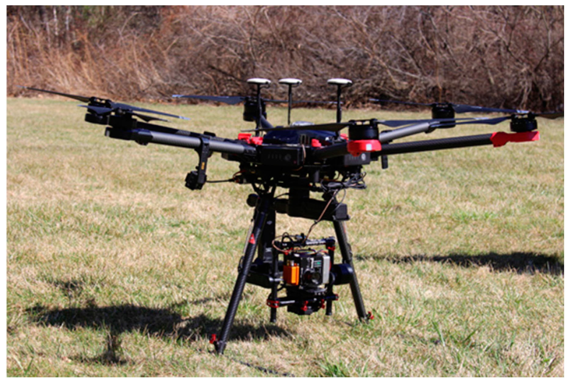
After consideration of the spectral and spatial requirements for most applications, the Micro-Hyperspec VNIR A-Series imager—exhibiting 1004 spatial pixels and 324 bands from 400 to 1000 nm at a maximum—was selected as the hyperspectral image acquisition instrument. Lucieer et al. [14] integrated a UAV hyperspectral system with the Micro-Hyperspec imager and other components on a multirotor UAV without a gimbal to provide extra stability; however, the synchronization between the imager and the GPS/IMU was not well designed. Jaud et al. [15] proposed a hyperspectral system named Hyper-DRELIO for a multirotor UAV by using the Micro-Hyperspec imager as a core component. Hyper-DRELIO adopted an IMU with high accuracy (0.05° for roll and pitch), which used a gimbal, and synchronized the imaging module and navigation module on the basis of central processing unit (CPU) timestamps. The Micro-Hyperspec imager employs an all-reflective and concentric optical layout to guarantee high spectral and spatial resolution and to minimize smiling and keystone effects; detailed specifications can be found in [3]. A six-rotor UAV was used because it offers the advantages of low cost and ease of operation. In addition to these two main devices, the GPS/IMU, stabilizing gimbal, and data acquisition and processing software were also integrated into the system (Figure 1). Figure 2 shows a photograph of the entire integrated system resting on the ground. Apart from the UAV, the other onboard devices had a total weight of ≈3.9 kg (the weights of Headwall hyperspectral imager plus lens, hyperspectral camera lens, GPS/IMU unit, data collection and storage unit (DCSU), global navigation satellite systems (GNSS) antenna, gimbal, and cables of 680, 74, 48.5, 515, 99.1, 2300, and 183.4 g). The batteries of the Matrice 600 Pro UAV allow 16 min of system function; however, the effective imaging duration cannot exceed 8–13 min to allow for the duration of the ascent, descent, and cushion phases. Considering the maximum frame rate of 90 HZ (50 HZ is a typical setting) of the hyperspectral imager and the maximum imaging flight duration of 13 min, the maximum data volume collected during one flight is ≈46 GB. Therefore, the storage capacity of the 64 GB CompactFlash (CF) card was enough to store the hyperspectral data.
The hyperspectral imager and GPS/IMU were combined and connected to the DCSU, which was controlled by the data acquisition software to acquire hyperspectral images and GPS/IMU data and store them in a CF card inserted into the DCSU. The three devices—imager, GPS/IMU, and DCSU—were mounted in a suitable stabilizing gimbal framework that enabled the imager to observe the ground surface nearly in the nadir direction with a relatively stable attitude. The gimbal was especially vital for pushbroom hyperspectral imagers such as Micro-Hyperspec, as it reduced the severe geometric distortion in the flight direction. The gimbal framework and the above three main devices were mounted on the UAV. The flight path, speed, and altitude of the UAV were controlled by the flight control software, which is usually provided by the UAV supplier. The maximum flight altitude of the Matrice 600 Pro could be above 2000 m (Table 1); however, a lower attitude is always selected to collect high-resolution data. The UAV’s speed, determined by the frame frequency and the instantaneous field of view (IFOV) of hyperspectral imager, as well as its flight altitude should be adjusted to avoid scanning gaps when collecting data. After data acquisition, data processing software was applied to the raw data to correct for geometric distortion and to derive the radiance or ground reflectance images. In addition, the software integrated an image mosaic function that helped to stitch several small images into a large-scale image. Some components of the system (i.e., imager, GPS/IMU, stabilizing gimbal, UAV, and its flight control software) were purchased from commercial companies. Table 1 lists their primary specifications. Other components such as the data acquisition software, DCSU, and data processing software were custom-made by the authors and are described in detail in the following subsections.
3. DCSU and Data Acquisition Software
The DCSU was connected to the hyperspectral imager and the GPS/IMU unit on the stabilizing gimbal. It communicated with the hyperspectral imager using a camera link cable, controlled the imager observation procedure, and exported data from the imager to the CF card inserted in the DCSU. It also communicated with the GPS/IMU via a universal serial bus (USB) cable and stored GPS/IMU data in its memory. To synchronize the imager and GPS/IMU, a pulse signal was sent by the imaging module to the GPS/IMU module just before each line was scanned. Then, each GPS/IMU signal recorded closest to the pulse sent by the imaging module was labeled and recorded together with the label of the corresponding line scanned. Further, the DCSU offered a port to connect with the UAV and to accept a signal from the UAV to determine whether to start or to stop the imager’s work. The total weight of the DCSU was ≈500 g. Figure 3 shows a structural schematic and a photograph of the DCSU.
A data acquisition software program was developed to allow the DCSU to drive the imager, GPS/IMU, and CF card, as well as to ensure that they worked properly after setting certain parameters such as the integration time, gain, and number of spectral bands for hyperspectral data collection. Further, the latest data collected by the GPS/IMU can be displayed on the software interface to help evaluate the accuracy of the position and attitude (Figure 4). It is advisable to begin data collection once the horizontal position accuracy surpasses 10 m. Then, the hyperspectral imager commenced operation upon receiving a pulse signal with a width greater than 1.6 ms. The hyperspectral data were stored in the CF card and could be output in the band interleaved by line (BIL) format by the data acquisition software. The original GPS/IMU data were automatically resampled to correspond with each scanning line of the hyperspectral data and transformed into American standard code for information interchange (ASCII) format after downloading hyperspectral data from the DCSU through the transfer software (Figure 4b). The GPS/IMU ASCII file was sent to the data processing software to perform geometric referencing of the image.
4. Data Processing Software
Owing to the complexity in UAV data acquisition conditions, basic data processing capabilities, especially in terms of radiance transform, surface reflectance computation, geometric referencing, and stripe stitching are very important in ensuring that the UAV hyperspectral data can be used for further quantitative applications. Although the principles of UAV data processing are generally similar to those of data processing for manned vehicles, specific adjustments are still needed for a better match with our hyperspectral data acquisition process. Figure 5 shows the main interface and main functions of the software.
4.1. Radiance and Surface Reflectance Computation
Periodic radiometric calibration of the hyperspectral imager in a laboratory is recommended. As a vital complementary component, the in situ experiment also provided an opportunity to ascertain the change in the radiometric performance of the UAV hyperspectral imager using recently developed methods [20,21,22]. The radiance image (L) was derived by subtracting dark currents (B) from the raw digital number image (DN), followed by the application of the gain coefficients (A), as follows:
where i, j, and k represent the column index, row index, and band index, respectively.
The gain coefficients and dark currents were automatically computed as intermediate parameters by the radiance computation module after inputting the dark current and radiance files from the laboratory calibration procedure.
A key step in the surface reflectance retrieval from remote sensing data is atmospheric correction (AC), which serves to reduce the absorption and scattering influence of aerosols and atmospheric molecules. Several AC-related algorithms, which can be divided into two categories (i.e., physical and empirical algorithms), have been developed in recent decades. On the basis of radiometric transfer codes such as 6SV [23] or MODTRAN [24], physical methods have been implemented in several typical commercial AC software packages—these include Atmospheric and Topographic Correction (ATCOR) [2,25,26], Atmospheric Correction Now (ACORN) [27], Fast Line-of-sight Atmospheric Analysis of Hypercubes (FLAASH) [28,29,30], and High-accuracy Atmospheric Correction for Hyperspectral Data (HATCH) [31]. One of the typical empirical methods is called the empirical line method (ELM); it uses the in situ reflectance measurements obtained over a pair of bright and dark objects to derive the atmospheric correction parameters [32]. The atmospheric variation in space can be ignored and the ELM works well over a small acquisition region [2]. A three-parameter empirical method was proposed to compensate for the multiple scattering effect (more evident in heavy aerosol burden conditions) ignored by the ELM method, as follows:
where L is the image radiance calculated by Equation (1); is the surface reflectance; A, B, and C are the transform coefficients between ground reflectance and the radiance measured by the UAV imager, representing path radiance, bottom atmospheric albedo, and an additional parameter depending on atmospheric and geometric conditions, respectively. Thus, at least three standard panels or tarps with different reflectances were placed within the flight area to derive these three parameters.
4.2. Georeferencing and Mosaicking
The UAV image acquired by the pushbroom imager showed evident geometric distortion, which is the biggest hindrance to its widespread application. Theoretically, the accurate position of each pixel can be predicted using the geometric parameters (i.e., focal length and physical pixel size), position and attitude parameters from the GPS/IMU, and relationship between the GPS/IMU and the imager (i.e., transform parameters between their individual coordinate systems) [33]. The principle used for the geometric correction of airborne pushbroom imagery applies to UAV imagery; however, the latter is more complex. Both the gimbal jitter and the measurement accuracy of the GPS/IMU affect the geometric referencing results of UAV pushbroom images [2]. Moreover, the UAV platform may move forward more slowly or quickly than expected, or even move backward suddenly, owing to strong atmospheric turbulence. Consequently, certain regions are scanned more or less frequently or even multiple times. Therefore, the current geometric referencing procedure cannot be directly applied to UAV pushbroom images. Given these factors, a modified georeferencing procedure was used, the steps of which are described below:
- (1)
- Screening the abnormal records in the GPS/IMU file. Table 2 lists the entries of a typical GPS/IMU file in ASCII format. The GPS/IMU records sometimes contain abnormal geographic position or attitude parameter values as a result of unknown factors. The abnormal values are very large (much more than 1.0 × 10¹⁰) in latitude, longitude, and height. Therefore, a simple criterion was set to screen them by determining whether the latitude and longitude values were out of a meaningful geographic scope (i.e., −180° to 180° of longitude and −90° to 90° of latitude). Finally, the abnormal values can be replaced by the average values of the adjacent lines.
- (2)
- Calculating the projected map coordinates for each pixel. This step is similar to the ordinate geometric referencing procedure used for manned airborne pushbroom images involving collinearity equations and including several coordinate transformations [15,34,35]. The focal length and physical pixel size and the expected projected map coordinate (e.g., Universal Transverse Mercator (UTM) or Gauss–Kruger coordinate) should be known after the image is georeferenced.
- (3)
- Resampling from original data. The geometric referencing results must be resampled into a regular grid. A resampling strategy is always used to find the accurate position in the original raw image for a certain pixel in the projected image space. One georeferencing method involving a geographic lookup table (GLT) developed by ENVI could work well for satellite data or manned airborne pushbroom images; however, it always failed for the UAV pushbroom images in our experience. An alternative strategy was to assign a reasonable value for the gridded pixel by using the nearest projected pixels or considering the weights of the surrounding pixels projected from the original image to the projected image space (Equation (3)):where P denotes the pixel in the projected image with the column index i and row index j; k (1, ..., n) refers to the index of the pixel projected within one pixel distance near P (i.e., from i-0.5 to i-0.5 and from j-0.5 to j + 0.5); G is the neighboring pixel of P(i, j) after being projected from the original image position () into the new position () of the projected image; and w is the weight of the pixel calculated by the area it contributes to the final pixel G. To avoid oversampling, it is recommended that the resampling resolution should not be set to a value higher than the real one determined by flight height, imager focal length, and pixel size.
- (4)
- Filling in the gaps using the neighbor pixels. Such gaps usually appear when wind gusts suddenly push the UAV forward at a speed that exceeds the speed expected according to its exposure time and flight height. Thus, it is better to fill in the gap lines by weighting the upper and lower valid pixels in the direction along the flight direction. In our resampling strategy, the georeferencing image was rotated at a certain angle to align the flight direction along the image column. The gap was much easier to fill by just using the pixels in the upper and lower rows.
After the georeferencing correction was completed for each flight strip, image mosaicking was used to combine small strips into a relatively large image. Owing to the limited geometric correction accuracy of the georeferencing image, the strips could not be stitched together using only their georeferenced coordinates. The scale-invariant feature transform (SIFT) features were first extracted and the geographic relationship between features in the overlapping area was used to filter out the obviously wrong matching features. Then, the RANSAC method, which was originally used for picture stitching [36], was further used to find optimal matching features between the two adjacent georeferenced flights of hyperspectral data. The stitching process was performed for all spectral bands of hyperspectral data as a subsequent step.
5. Results
The whole system was tested using several flight experiments and data processing tests designed to improve its robustness. Two typical experiments are described below to demonstrate the data acquisition and processing results.
5.1. Zhuozhou Experiment
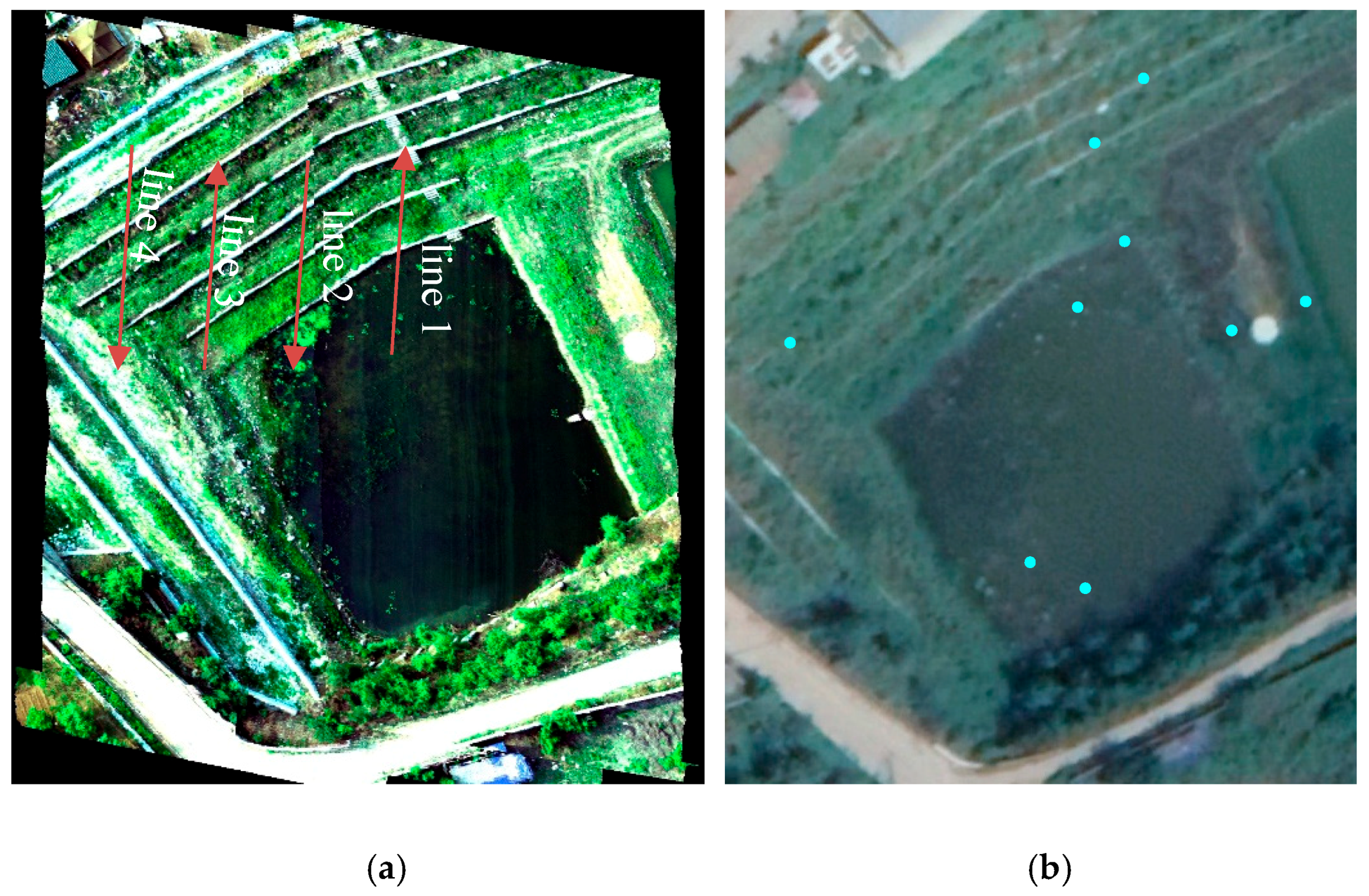
The system was evaluated following the first flight experiment conducted over Zhuozhou (39°33′16.8″N, 115°47′47.1″E), China, on 18 May 2018. Four flight strips were acquired; however, the stabilizing gimbal did not function in this experiment. Consequently, evident distortion can be found in the original images. A camera lens with a focal length of 17 mm was used and the flight height above the ground was ≈170 m. The ground resolution of the image is 0.055 m. Figure 6 shows the flight strips before and after georeferencing. Figure 7 shows a comparison of the mosaicked image with the satellite image acquired on 17 April 2018, from Google Earth. The results indicated a reliable UAV hyperspectral acquisition system and satisfactory data processing results, although the GPS/IMU did not have a very high accuracy and the stabilizing gimbal failed to function.
5.2. Hong Kong Experiment
A flight experiment was performed to verify the performance of the whole system further over Hong Kong (22°29′00″N, 114°02′04.5″E) on 7 August 2018. A camera lens with a focal length of 8 mm was used and nine flight strips were acquired. The flight height above the ground was ≈320 m and the ground resolution of the image is 0.324 m. The stabilizing gimbal worked well, and even the original image did not show high-frequency distortion among image rows. Figure 8 and Figure 9 respectively show the first four strips before and after georeferencing and the result of mosaicking nine strips.
5.3. Geometric Correction Accuracy Evaluation
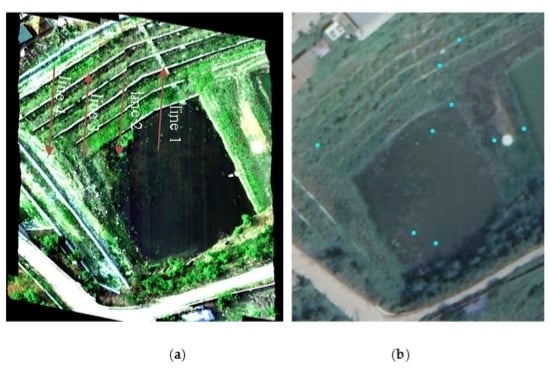
Owing to the lack of the ground measured ground control points (GCPs), the absolute georeferencing accuracy was impossible to evaluate. However, the SkySat ortho images with spatial resolution of 1.0 m and position accuracy of less than 10 m [37] were used to evaluate the geometric accuracy of the georeferencing images acquired over Zhuozhou and Hong Kong (Figure 6 and Figure 8). With 9 and 25 selected controls points (Figure 7b and Figure 9b), the horizontal root mean square error (RMSE) of the georeferencing results were 5.26 and 7.49 m in the Zhouzhou and Hong Kong experiments, respectively. Although such accuracy estimation was not based on in situ measurements of the control points, it still provided a reference for the absolute geometric accuracy of the georeferencing results.
In addition, the relative georeferencing accuracy between the adjacent flight lines was assessed by using the same featured points in their overlap area. More matching points could be easily found in the larger overlap region. Therefore, over 50 and 7–9 points were selected for evaluating the relative geometric accuracy of images acquired over Zhuozhou and Hong Kong, respectively. The results (Figure 10) show that the relative geometric positions differred by 10–40 pixels (0.7–1.5 m and 2.7–13.1 m for Zhuozhou and Hong Kong, respectively) between two adjacent fight lines. However, the relative position errors varied with different flight lines, for which the accuracy was likely to be affected by boresight error, orientation parameter measured errors, and flight conditions. Similar findings were also reported by other researchers [15].
6. Discussion
The integrated system constitutes a stable hyperspectral data acquisition and processing solution, as proved by several experiments. We focused on the two significant process steps of the UAV onboard pushbroom imager, namely, georeferencing and surface reflectance retrieval. A stabilizing gimbal and a GPS/IMU with moderate accuracy were mounted on the UAV to minimize the apparent geometric distortion. Reasonable georeferencing results were achieved in the Zhuozhou and Hong Kong experiments with the optimal geometric referencing method, even though the stabilizing gimbal failed to function in the former case. The mosaicked UAV image was very similar to a high-resolution satellite image in terms of geometric characteristics. As a comparison, the orthorectified result (Figure 11) in [14] still shows evident geometric distortion as judged from the measuring tape owing to the lack of a stabilizing gimbal and high-frequency GPS/IMU. Additionally, this orthorectified image contained many gaps.
For further discussion, the dataset acquired in the Zhuozhou experiment was used as an example. The altitude changed significantly at the end or beginning of each flight strip (red rectangles in Figure 6), and the raw image in these regions appeared to be almost unusable. It is hard to recognize the roof of the building in the lower right corner of Figure 6g (corresponding to the upper left corner of Figure 6h). Figure 11a shows data for the UAV course reversal at the beginning of the flight strip for Figure 6g.
Usually, it is hard to process the overlap data unless the overlap flight images are separated. In addition, the roll angles changed drastically, indicating that the UAV shook dramatically, which was the main reason for the geometric distortion shown in the images acquired during the Zhuozhou experiment. However, our refined georeferencing strategy permitted processing without separating or discarding overlapping flight image parts.
The longitude and latitude positions of each pixel were easy to compute using collinear equations (Figure 12) [33]. The map of the longitude and latitude for each pixel further showed the complicated geometric distortions of the UAV pushbroom images, especially in the case without the stabilizing gimbal. We used the geographic position file to generate a GLT file and then used ENVI software to perform geometric referencing of the raw data; however, this process failed. This failure was attributed primarily to the fact that the geographic positions of the pixels in the UAV image did not change continuously. Furthermore, the gap-filling step following image georeferencing was used to avoid spatial discontinuity when the UAV was suddenly pushed forward by wind gusts.
Additionally, the PARGE software [34] was used to process these data, and the georeferencing results matched those obtained using our methods. However, one georeferencing image processed by PARGE contained gaps not seen in the image processed using our methods (Figure 13).
Pushbroom image stitching can still be improved not only because the image georeferencing accuracy was not high enough but also because the accuracy was not consistent across scanning lines. Although the RANSAC method was used to build the transform relations between adjacent strips, the stitching was still problematic in areas without many features such as roads and buildings. In the future, it would be beneficial to add a small frame camera to assist in refining the external oriental parameters (i.e., position and angle parameters) of each scan line of the pushbroom images following initial georeferencing using the GPS/IMU data [38]. By doing this, different strips acquired by the UAV can be stitched together with satisfactory accuracy.
The traditional ELM is always applied to imagery acquired over a small area. As a comparison, the three-parameter ELM was used to derive the surface reflectance from the UAV imagery acquired by the Micro-Hyperspec imager over Baoding (38.87°N, 115.33°E), Hebei province, China, on 28 June 2014 [21]. During the experiment, the reflectances were measured over the three tarps (i.e., with reflectances of 5%, 20%, and 60%, respectively) and the black mesh was measured (Figure 14a). Three tarp reflectances were used in three-parameter ELM to derive coefficients in Equation (2) and to compute the surface reflectance accordingly. Meanwhile, two tarps with reflectances of ≈20% and 60% were used in traditional ELM. The retrieved reflectance of the black mesh by the two methods was compared with the in situ measured reflectance (Figure 14b). The retrieved reflectance by the three-parameter ELM was closer to the measured reflectance, with an REMS of 0.38% in the spectral range before 902 nm compared with that of 2.0% by the traditional ELM. The three-parameter ELM compensated for the multiple scattering effect between the ground and the atmosphere, which was more evident when the aerosol optical depth (AOD) became large. As mentioned in [21], the AOD at 550 nm was 0.54 on the day when data were acquired in the experiment in Baoding. Therefore, the multiple scattering effect between the ground and the bottom of the atmosphere could not be ignored. The three-parameter ELM is recommended to derive the reflectance of UAV imagery, especially in non-ideal weather conditions.
7. Conclusions
We presented herein a lightweight integrated solution for a UAV-mounted hyperspectral imaging system. The data acquisition system integrated a hyperspectral imager, GPS/IMU system, stabilizing gimbal, and DCSU. Postprocessing software was developed to transform the raw data into the radiometric and geometric rectified radiance and surface reflectance data. Further, the mosaic result obtained by stitching different strips together using the present algorithm was of limited accuracy and will be further improved after adding a red-green-blue (RGB) frame camera. The whole system achieved satisfactory performance by optimizing the tradeoff among factors such as actual application requirements, device weight, and instrument specifications. Although the pushbroom hyperspectral imager has inherent deficiencies in geometric rectification, we chose to use this type of imager in the system because of its superior spectral performance and its wide spatial dimensions (e.g., the Headwall Micro-Hyperspec has 1004 pixels). The geometric distortion of the image was significantly reduced by the stabilizing gimbal unit and the postprocessing geometric correction software unit.
Moreover, the boresight of the hyperspectral imager relative to the GPS/IMU should be calibrated to make the whole system achieve better geometric accuracy. Further, the GPS/IMU with a higher attitude measurement accuracy (0.05° for roll and pitch of SBG System Ekinox-D IMU) was very helpful for minimizing the high-frequency vibration of the UAV image. In the future, an RGB frame camera will be added to the system to further increase the consistency in terms of geometric accuracy among different scanning lines and reduce stitching errors between adjacent strips.
Author Contributions
H.Z., B.Z., and Z.W. conceptualized the whole system. Q.H. and C.W. performed the experiments and collected relevant data. H.Z. and Q.H. processed the data. H.Z. contributed to the analysis and discussion and wrote the paper. All authors have read and agreed to the published version of the manuscript.
Funding
National Key R&D Program of China: 2016YFB0500301; National Natural Science Foundation of China: 41771397; National Key R&D Program of China: 2016YFB0500304; National Key R&D Program of China: 2016YFD0300603.
Acknowledgments
This research was supported by the National Key R&D Program of China (2016YFB0500301), National Natural Science Foundation of China (41771397), and National Key R&D Program of China (2016YFB0500304 and 2016YFD0300603). We thank ReSe Applications LLC (https://www.rese-apps.com/software/index.html) for providing the PARGE trial to process the UAV data. We also thank Ambit Geospatial Solution (www.ambit-geospatial.com.hk) for their assistance in the data acquisition and field experiments. Further, we would like to thank Editage (www.editage.cn) for English language editing.
Conflicts of Interest
The authors have no conflict of interest to declare.
References
- Colomina, I.; Molina, P. Unmanned aerial systems for photogrammetry and remote sensing: A review. ISPRS J. Photogramm. Remote Sens. 2014, 92, 79–97. [Google Scholar] [CrossRef] [Green Version]
- Zhong, Y.; Wang, X.; Xu, Y.; Wang, S.; Jia, T.; Hu, X.; Zhao, J.; Wei, L.; Zhang, L. Mini-UAV-Borne Hyperspectral Remote Sensing: From Observation and Processing to Applications. IEEE Geosci. Remote Sens. Mag. 2018, 6, 46–62. [Google Scholar] [CrossRef]
- Photonics. Available online: http://www.headwallphotonics.com (accessed on 22 May 2019).
- Cubert. Available online: https://cubert-gmbh.com/spectral-cameras/ (accessed on 22 May 2019).
- BaySpec. Available online: https://www.bayspec.com (accessed on 22 May 2019).
- SENOP. Available online: https://senop.fi/en/optronics-hyperspectral (accessed on 7 October 2019).
- Adão, T.; Hruška, J.; Pádua, L.; Bessa, J.; Peres, E.; Morais, R.; Sousa, J. Hyperspectral Imaging: A Review on UAV-Based Sensors, Data Processing and Applications for Agriculture and Forestry. Remote Sens. 2017, 9, 1110. [Google Scholar] [CrossRef] [Green Version]
- Gao, L.; Smith, R.T. Optical hyperspectral imaging in microscopy and spectroscopy - a review of data acquisition. J. Biophotonics 2015, 8, 441–456. [Google Scholar] [CrossRef] [PubMed] [Green Version]
- Strauch, M.; Livshits, I.L.; Bociort, F.; Urbach, H.P. Wide-angle spectral imaging using a Fabry-Pérot interferometer. J. Eur. Opt. Soc. Rapid Publ. 2015, 10. [Google Scholar] [CrossRef] [Green Version]
- Mäkeläinen, A.; Saari, H.; Hippi, I.; Sarkeala, J.; Soukkamäki, J. 2D Hyperspectral frame imager camera data in photo- grammetric mosaicking. In Proceedings of the ISPRS International Archives of the Photogrammetry, Remote Sensing and Spatial Information Sciences (UAV-g2013), Rostock, Germany, 4–6 September 2013; Volume XL-1/W2, pp. 263–268. [Google Scholar]
- Bareth, G.; Aasen, H.; Bendig, J.; Gnyp, M.L.; Bolten, A.; Jung, A.; Michels, R.; Soukkamäki, J. Low-weight and UAV-based Hyperspectral Full-frame Cameras for Monitoring Crops: Spectral Comparison with Portable Spectroradiometer Measurements. Photogramm. Fernerkund. Geoinf. 2015, 2015, 69–79. [Google Scholar] [CrossRef]
- Nano-Hyperspec. Available online: https://cdn2.hubspot.net/hubfs/145999/Nano-Hyperspec_Oct19.pdf (accessed on 22 May 2019).
- Hill, S.L.; Clemens, P. Miniaturization of sub-meter resolution hyperspectral imagers on unmanned aerial systems. In Proceedings of the SPIE 9104, Spectral Imaging Sensor Technologies: Innovation Driving Advanced Application Capabilities, Baltimore, MD, USA, 28 May 2014. [Google Scholar]
- Lucieer, A.; Malenovský, Z.; Veness, T.; Wallace, L. HyperUAS-Imaging Spectroscopy from a Multirotor Unmanned Aircraft System. J. Field Robot. 2014, 31, 571–590. [Google Scholar] [CrossRef] [Green Version]
- Jaud, M.; Le Dantec, N.; Ammann, J.; Grandjean, P.; Constantin, D.; Akhtman, Y.; Barbieux, K.; Allemand, P.; Delacourt, C.; Merminod, B. Direct Georeferencing of a Pushbroom, Lightweight Hyperspectral System for Mini-UAV Applications. Remote Sens. 2018, 10, 204. [Google Scholar] [CrossRef] [Green Version]
- Hyperspec® MV.X. Available online: https://www.headwallphotonics.com/hyperspectral-sensors (accessed on 9 October 2019).
- SBG Ellipse2-N. Available online: http://www.canalgeomatics.com/product/ellipse2-n-miniature-ins-gps/?gclid=Cj0KCQjwivbsBRDsARIsADyISJ8QVollVsPQDd7fwsE3kyzeD4t7EYZZMP1EmcBE5x1lUiNMp8n8YEAaAmmcEALw_wcB (accessed on 9 October 2019).
- Ronin-MX. Available online: https://www.dji.com/ronin-mx/info#specs (accessed on 9 October 2019).
- Matrice 600 Pro. Available online: https://www.dji.com/matrice600-pro/info#specs (accessed on 9 October 2019).
- Zhang, H.; Zhang, B.; Chen, Z.; Huang, Z. Vicarious Radiometric Calibration of the Hyperspectral Imaging Microsatellites SPARK-01 and -02 over Dunhuang, China. Remote Sens. 2018, 10, 120. [Google Scholar] [CrossRef] [Green Version]
- Haiwei, L.; Hao, Z.; Bing, Z.; Zhengchao, C.; Minhua, Y.; Yaqiong, Z. A Method Suitable for Vicarious Calibration of a UAV Hyperspectral Remote Sensor. IEEE J. Sel. Top. Appl. Earth Obs. Remote Sens. 2015, 8, 3209–3223. [Google Scholar] [CrossRef]
- Brook, A.; Polinova, M.; Ben-Dor, E. Fine tuning of the SVC method for airborne hyperspectral sensors: The BRDF correction of the calibration nets targets. Remote Sens. Environ. 2018, 204, 861–871. [Google Scholar] [CrossRef]
- Kotchenova, S.Y.; Vermote, E.F.; Levy, R.; Lyapustin, A. Radiative transfer codes for atmospheric correction and aerosol retrieval: Intercomparison study. Appl. Opt. 2008, 47, 2215–2226. [Google Scholar] [CrossRef] [PubMed] [Green Version]
- Berk, A.; Conforti, P.; Kennett, R.; Perkins, T.; Hawes, F.; Bosch, J.v.d. MODTRAN® 6: A major upgrade of the MODTRAN® radiative transfer code. In Proceedings of the 2014 6th Workshop on Hyperspectral Image and Signal Processing: Evolution in Remote Sensing (WHISPERS), Lausanne, Switzerland, 24–27 June 2014; pp. 1–4. [Google Scholar]
- Richter, R. Correction of atmospheric and topographic effects for high spatial resolution satellite imagery. Int. J. Remote Sens. 1997, 18, 1099–1111. [Google Scholar] [CrossRef]
- Richter, R.; Schläpfer, D. Atmospheric/Topographic Correction for Satellite Imagery: ATCOR-2/3 User Guide. Available online: http://www.rese.ch/pdf/atcor3_manual.pdf (accessed on 12 February 2020).
- Miller, C.J. Performance assessment of ACORN atmospheric correction algorithm. In Proceedings of the SPIE 4725, Algorithms and Technologies for Multispectral, Hyperspectral, and Ultraspectral Imagery VIII, Orlando, FL, USA, 2 August 2002. [Google Scholar] [CrossRef]
- Matthew, M.W.; Adler-Golden, S.M.; Berk, A.; Richtsmeier, S.C.; Levine, R.Y.; Bernstein, L.S.; Acharya, P.K.; Anderson, G.P.; Felde, G.W.; Hoke, M.L.; et al. Status of atmospheric correction using a MODTRAN4-based algorithm. In Proceedings of the SPIE 4049, Algorithms for Multispectral, Hyperspectral, and Ultraspectral Imagery VI, Orlando, FL, USA, 23 August 2000. [Google Scholar] [CrossRef]
- Anderson, G.P.; Pukall, B.; Allred, C.L.; Jeong, L.S.; Hoke, M.; Chetwynd, J.H.; Adler-Golden, S.M.; Berk, A.; Bernstein, L.S.; Richtsmeier, S.C.; et al. FLAASH and MODTRAN4: state-of-the-art atmospheric correction for hyperspectral data. In Proceedings of the 1999 IEEE Aerospace Conference, Proceedings (Cat. No. 99TH8403), Aspen, CO, USA, 7 March 1999; Volume 174, pp. 177–181. [Google Scholar]
- Adler-Golden, S.M.; Matthew, M.W.; Bernstein, L.S.; Levine, R.Y.; Berk, A.; Richtsmeier, S.C.; Acharya, P.K.; Anderson, G.P.; Felde, J.W.; Gardner, J.A.; et al. Atmospheric correction for shortwave spectral imagery based on MODTRAN4. In Proceedings of the SPIE 3753, Imaging Spectrometry V, Denver, CO, USA, 27 October 1999. [Google Scholar] [CrossRef]
- Zheng, Q.; Kindel, B.C.; Goetz, A.F.H. The High Accuracy Atmospheric Correction for Hyperspectral Data (HATCH) model. IEEE Trans. Geosci. Remote Sens. 2003, 41, 1223–1231. [Google Scholar] [CrossRef]
- Smith, G.M.; Milton, E.J. The use of the empirical line method to calibrate remotely sensed data to reflectance. Int. J. Remote Sens. 2010, 20, 2653–2662. [Google Scholar] [CrossRef]
- Turner, D.; Lucieer, A.; McCabe, M.; Parkes, S.; Clarke, I. Pushbroom Hyperspectral Imaging from an Unmanned Aircraft System (Uas) – Geometric Processingworkflow and Accuracy Assessment. Isprs - Int. Arch. Photogramm. Remote Sens. Spat. Inf. Sci. 2017, XLII-2/W6, 379–384. [Google Scholar] [CrossRef] [Green Version]
- Schläpfer, D.; Richter, R. Geo-atmospheric processing of airborne imaging spectrometry data. Part 1: Parametric orthorectification. Int. J. Remote Sens. 2010, 23, 2609–2630. [Google Scholar] [CrossRef]
- Gabrlik, P.; Cour-Harbo, A.l.; Kalvodova, P.; Zalud, L.; Janata, P. Calibration and accuracy assessment in a direct georeferencing system for UAS photogrammetry. Int. J. Remote Sens. 2018, 39, 4931–4959. [Google Scholar] [CrossRef] [Green Version]
- Fischler, M.A.; Bolles, R.C. Random sample consensus: A paradigm for model fitting with applications to image analysis and automated cartography. Commun. ACM 1981, 24, 381–395. [Google Scholar] [CrossRef]
- Planet. Planet Imagery Product Specifications. Available online: https://assets.planet.com/docs/Planet_Combined_Imagery_Product_Specs_letter_screen.pdf (accessed on 16 March 2019).
- Barbieux, K. Pushbroom Hyperspectral Data Orientation by Combining Feature-Based and Area-Based Co-Registration Techniques. Remote Sens. 2018, 10, 645. [Google Scholar] [CrossRef] [Green Version]
Figure 1.
Scheme of unmanned aerial vehicle (UAV) hyperspectral imaging system integration.

Figure 2.
Photograph of UAV hyperspectral imaging system.

Figure 3.
(a) Schematic and (b) photograph of data collection and storage unit (DCSU).

Figure 4.
Interface of (a) data acquisition software and (b) data transfer software.

Figure 5.
Main interface of processing software.

Figure 6.
Four flight image strips (a,c,e,g) before and (b,d,f,h) after georeferencing shown in true color with infrared, red, and green bands. Figure 6b,d,f,h show the results of rotating the georeferenced images clockwise by 350.64°, 349.11°, 348.35°, and 348.80°, respectively.. The red rectangles show the severe distortion area in each flight strip.

Figure 7.
Comparison of the (a) mosaicked image by stitching Figure 6b,d,f,h with the (b) satellite image acquired on 4 September 2018, from Google Earth.
Figure 7.
Comparison of the (a) mosaicked image by stitching Figure 6b,d,f,h with the (b) satellite image acquired on 4 September 2018, from Google Earth.

Figure 8.
Four flight image strips (a,c,e,g) before and (b,d,f,h) after georeferencing shown in pseudo color with infrared, red, and green bands. Figure 8b,d,f,h show the results of rotating the georeferenced images clockwise by 239.61°, 65.07°, 241.74°, and 64.26°, respectively.
Figure 8.
Four flight image strips (a,c,e,g) before and (b,d,f,h) after georeferencing shown in pseudo color with infrared, red, and green bands. Figure 8b,d,f,h show the results of rotating the georeferenced images clockwise by 239.61°, 65.07°, 241.74°, and 64.26°, respectively.

Figure 9.
Comparison of (a) mosaicked image with a (b) satellite image acquired on 28 October 2018 from Google Earth.
Figure 9.
Comparison of (a) mosaicked image with a (b) satellite image acquired on 28 October 2018 from Google Earth.

Figure 10.
Relative georeferencing errors between two adjacent images (a) acquired over Zhouzhou (lines 1–4 are labeled in Figure 7) and (b) acquired over Hong Kong (lines 1–9 are labeled in Figure 9).


Figure 11.
Part of flight GPS/INS data in last 500 rows in Figure 6g: (a) latitude and longitude data and (b) rolling angles.
Figure 11.
Part of flight GPS/INS data in last 500 rows in Figure 6g: (a) latitude and longitude data and (b) rolling angles.

Figure 12.
Geographic positions for each pixel in Figure 6g: (a) latitude values and (b) longitude values.
Figure 12.
Geographic positions for each pixel in Figure 6g: (a) latitude values and (b) longitude values.

Figure 13.
Georeferencing imagery of flight line 7 (Figure 9a) acquired over Hong Kong processed by (a) PARGE and (b) our method.
Figure 13.
Georeferencing imagery of flight line 7 (Figure 9a) acquired over Hong Kong processed by (a) PARGE and (b) our method.

Figure 14.
Part of the data acquired over Baoding in 2014 and retrieval results: (a) pixels in rectangles were used for surface reflectance retrieval and validation, and (b) comparison of retrieval results with in situ measurement.
Figure 14.
Part of the data acquired over Baoding in 2014 and retrieval results: (a) pixels in rectangles were used for surface reflectance retrieval and validation, and (b) comparison of retrieval results with in situ measurement.


Table 1.
Main specifications for some components of the hyperspectral UAV system.
| Component | Parameter | Specification |
|---|---|---|
| Imager (Headwall Micro-Hyperspec VNIR A-Series [16]) | Wavelength | 400–1000 nm |
| Spatial pixels | 1004 | |
| Bit depth | 12-bit | |
| Full width at half maximum (max.) (FWHM) | 5.8 nm | |
| Frame rate | ≥30 HZ | |
| Pixel size | 7.4 µm | |
| Focal plane array | Silicon CCD | |
| Weight | 0.68 kg | |
| Signal-to-noise ratio (SNR) | ≥60 | |
| GPS/IMU (SBG Ellipse2-N [17]) | Roll and pitch accuracy | 0.1° |
| Heading accuracy | 0.5° | |
| Position accuracy | 2 m | |
| Output rate | 200 HZ | |
| Weight | 47 g | |
| Gimbal (DJI Ronin-MX 3-Axis Gimbal Stabilizer [18]) | Rotation range | pitch: −150°–270° roll: −110°–110° yaw: 360° |
| Follow speed | pitch: 100°/s roll: 30°/s yaw: 200°/s | |
| Stabilization accuracy | ±0.02° | |
| Weight | 2.15 kg | |
| Load capacity | 4.5 kg | |
| UAV (Matrice 600 Pro [19]) | Dimensions (mm) | 1668 (L) × 1518 (W) × 727 (H) |
| Weight (with batteries) | 10 kg | |
| Max. takeoff weight | 15.5 kg | |
| Max. speed | 65 km/h (no wind) | |
| Hovering Accuracy | Vertical: ±0.5 m, horizontal: ±1.5 m | |
| Max. Wind Resistance | 8 m/s | |
| Max. Service Ceiling Above Sea Level | 2500 m by 2170R propellers; 4500 m by 2195 propellers | |
| Operating temperature | −10 to 40 °C | |
| Max. transmission distance | 3.5 km |
Table 2.
Entries recorded by global-positioning system combined with an inertial measurement unit (GPS/IMU) file in ASCII format.
Table 2.
Entries recorded by global-positioning system combined with an inertial measurement unit (GPS/IMU) file in ASCII format.
| Item | Unit | Data Type | Meaning | Example |
|---|---|---|---|---|
| No. | none | Integer | Row number of the image | 2948 |
| Time | none | String (yyyy/mm/dd hh:mm:ss) | Exposure time | 2018/05/18 15:21:49.424900 |
| Longitude | degree | Double | Geographic longitude | 121.9721375 |
| Latitude | degree | Double | Geographic latitude | 31.53649527 |
| Altitude | meter | Double | Elevation above sea level | 108.6938 |
| Roll | degree | Float | Roll angle | −1.38 |
| Pitch | degree | Float | Pitch angle | 2.21 |
| Yaw | degree | Float | Yaw angle | 150.68 |
© 2020 by the authors. Licensee MDPI, Basel, Switzerland. This article is an open access article distributed under the terms and conditions of the Creative Commons Attribution (CC BY) license (http://creativecommons.org/licenses/by/4.0/).
Share and Cite
MDPI and ACS Style
Zhang, H.; Zhang, B.; Wei, Z.; Wang, C.; Huang, Q. Lightweight Integrated Solution for a UAV-Borne Hyperspectral Imaging System. Remote Sens. 2020, 12, 657. https://0-doi-org.brum.beds.ac.uk/10.3390/rs12040657
AMA Style
Zhang H, Zhang B, Wei Z, Wang C, Huang Q. Lightweight Integrated Solution for a UAV-Borne Hyperspectral Imaging System. Remote Sensing. 2020; 12(4):657. https://0-doi-org.brum.beds.ac.uk/10.3390/rs12040657
Chicago/Turabian StyleZhang, Hao, Bing Zhang, Zhiqi Wei, Chenze Wang, and Qiao Huang. 2020. "Lightweight Integrated Solution for a UAV-Borne Hyperspectral Imaging System" Remote Sensing 12, no. 4: 657. https://0-doi-org.brum.beds.ac.uk/10.3390/rs12040657
Note that from the first issue of 2016, this journal uses article numbers instead of page numbers. See further details here.