Infrasound Observations of Atmospheric Disturbances Due to a Sequence of Explosive Eruptions at Mt. Shinmoedake in Japan on March 2018

Abstract

Thirty infrasound sensors have been operated over Japan since 2015. We developed the irregular array data processing in order to detect and estimate the parameters of the arrival source waves by using infrasound data related to the sequence of the volcanic eruption at Mt. Shinmoedake in March 2018. We found that the apparent velocity at the ground was equal to the acoustic velocity at particular reflection levels. The results were confirmed through a comparison of the findings of the apparent velocity with a wave propagation simulation on the basis of the azimuth, infrasound time arrivals, and the state of the atmospheric background using global atmospheric models. In addition, simple ideas for estimating horizontal wind speeds at certain atmospheric altitudes based on infrasound observation data and their validation and comparison were presented. The calculated upper wind speed and wind observed by radiosonde measurements were found to have a qualitative agreement. Propagation modeling for these events estimated celerities in the propagation direction to the sensors that were consistent with the tropospheric and stratospheric ducting. This study could inspire writers, in particular, and readers, in general, to take advantage of the benefits of infrasound wave remote-sensing for the study of the Earth’s atmospheric dynamics.

1. Introduction

Infrasound is classified as sound waves with frequencies below the ${}^{\prime }$normal${}^{\prime }$ limit of human hearing and is often cited as the frequency range 0.02–10 Hz [1]. These waves are generated from various human-made and natural sources and can propagate efficiently over regional and global scales of thousands of kilometers, with low intrinsic attenuation [2,3]. For instance, very large sources (e.g., massive volcanic eruptions) can produce inaudible waves dominated by very low frequencies, particularly in the near-infrasonic range of 1–20 Hz [4], and were found to be well-correlated across a local network, suggesting a contribution from point source infrasound [5].

The advantages of infrasound waves have been exploited by researchers studying the characteristics of sound sources across the globe. Since 2015, in a collaboration between national industries and the Earth Space and Exploration System Laboratory (ESESL) of Kochi University of Technology (KUT) in Japan, new instrument designs have been developed to increase land-use efficiency and integrate surface meteorological measurements with seismology components. In addition, the system has been deployed for operation in various locations in Japan, especially in the Shikoku Island region. Since the observation network was established, our sensors have successfully detected and recorded several natural phenomena that produced infrasound waves (e.g., explosive volcanic eruptions and an intense earthquake that occurred in Japan). Three explosive volcanic eruptions were detected by the sensor, at Mt. Aso in 2016, Mt. Sakurajima in 2017, and Mt. Shinmoedake in 2018.

The majority of high-amplitude volcanic infrasound is attributable to the eruptive acceleration of compressed volatiles from vents [5,6]. Such infrasound may result from either a long period of acceleration of erupted gas from a compact vent or from an impulsive source distributed over a large region. In both cases, it is possible to detect infrasound from the eruption. There have been several previous reports of infrasonic observations likely caused by volcanic eruptions. One of these reports was based on the examination of air pressure data from one station, combined with a verification method implemented at another station (i.e., cross-correlation) [7,8]. Other reports were based on the evaluation of air pressure measurements from small-array sensors at locations close to the mountain cauldron (i.e., <10 km) [4,9,10,11] and analyses of the International Monitoring System (IMS) infrasound network [12,13,14,15,16,17,18,19,20] using the progressive multi-channel correlation (PMCC) technique [21,22]. Similar way in Russia [23], Italy [24,25], and Ecuador [10] also detected lower frequency waves associated with volcanic eruptions, in which air pressure disturbances traveled radially and uniformly away from source points. In general, the sensor array system used is relatively close to the observed source point (d < 10 km) with a fairly homogeneous distance between sensors (close and equal distances). These investigations found some clear changes in air pressure originating from volcanic eruptions, with amplitudes of >20 Pa. However, the propagation speeds inferred from the infrasonic detection (0.02–0.05 Hz) reported in above previous studies varied considerably, with apparent velocities ranging from ∼338 to ∼420 m/s.

A common objective in infrasound data processing is the estimation of the arrival direction (azimuth) of the incoming signals. Several methods for determining the azimuth of a source have been implemented. Frequency-wavenumber (f-k) analysis in combination with delay and sum beamforming in the time domain of the incoming signals [26], using the PMCC algorithm [21,27], computes time delays and uses the sum of the delays between unique sensor pairs to establish relationships for estimation of the arrival direction of the source for each window of the data. These methods are conducted using regular arrays of closely spaced sensors. Recently, our lab carried out three-dimensional ray-tracing using the vertical of atmospheric profiles, e.g., horizontal wind and temperature, to figure out the sound propagation profiles.

This work primarily focused on the development new methods and their applications by using remote sensing with infrasound waves through the utilization of infrasound data analysis for studying the upper atmosphere. We focused on powerful transient signals that travel through the atmosphere, which provided us with a quantitative basis to estimate infrasound specifications through a Radar Beam Swinging method implementation into our infrasound data processing. Here, we present our findings on far field infrasound returns from Mnt. Shinmoedake in Japan (31.9098°N, 130.8863°E), which was observed during sequences of explosive activity in March 2018. These explosions have estimated results in a strong explosive range. The identified source was then used to estimate the horizontal atmospheric wind velocity at certain altitude from recorded signal properties. Depending on the background atmospheric condition at low-mid altitude, the arrival signals are observed during sequence of explosive volcanic activities. It was also found that the comparison of the atmospheric wind speed between the infrasound observation and the radiosonde observation are relatively in good agreement. It was also found that the comparison of the atmospheric wind speed between the infrasound observation and the radiosonde observation are relatively in good agreement. Additionally, the implementation of the Radar Beam Swinging into our infrasound sensor array system gives a possible way to detect the source waves for further atmospheric wind estimation, even though it still meets several limitation during the processing. However, our results suggest the utilities of infrasound techniques could be used for atmospheric study.

This manuscript is structured as follows. An overview of the infrasound network used in this study is described in Section 2. Section 3 provides a description of the instrument specifications, which is followed by a description of the data set in Section 4. The selection of the data is described in Section 5. Details of the evaluation tools used in the methodology are given in Section 6. The results and discussion focus on the potential use of the infrasound network for geophysical variability analyses of our findings regarding atmospheric disturbances.

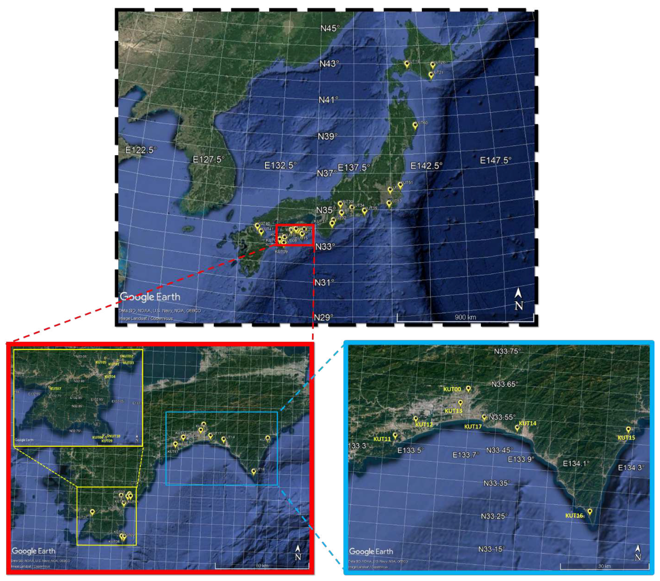
2. Infrasound Station Sites

The first operation of an infrasound sensor in Kuroshio city in Kochi prefecture occurred in 2016, following careful evaluation of the individual sensor performance. Currently, a total of 30 infrasound sensors are distributed uniformly over the Japanese islands and are in continuous operation. Providing an information about natural disaster such especially as earthquake and tsunami over the Shikoku region, the network likewise uses two different types compact sensors to ensure the detection of infrasound waves generated by both natural and man-made activities. The Japanese infrasound station network is shown in Figure 1, with their geographic coordinates listed in Table S1 in the supporting information. The network is denser on Shikoku Island, where it is used for the detection of natural disasters, such as tsunamis and volcanic eruptions.

3. Overall Description of the Instrument

Since 2005, KUT has collaborated with several local institutions in an initiative to build an infrasound sensor that is integrated with several micro-electro-mechanic system (MEMS) sensors to measure 3-axis acceleration in seismic waves, atmospheric temperature, atmospheric pressure, and the level of audible noise. The sensor system is also equipped with a signal processing unit for continuous real-time processing and network-connecting ports for data acquisition [28].

A full description of the specifications of the infrasound instrument is given in Table S2 in the supporting information and can be found in the company’s website [29]. The infrasound system, consisting of four types of high sensitivity sensors with additional of a dynamic data logger and a high speed digitizer, which is able to monitor the ambient condition of the environment (e.g., ground acceleration, local temperature, audible noise level, atmospheric pressure, and sound pressure level) and is therefore flexible to control through the internet connection. In 2016, we announced a total of five infrasound sensors were installed as a model area, and in 2017 we expanded the network to a total of 15 locations along the coastal area in Kochi Prefecture, and built a network to detect the arrival of tsunami-induced infrasound from the land surface.

At almost all stations, the four parameters are continuously digitized at 4 Hz by each individual sensor. The instrument was specially designed to be windproof and easy to install.

The sensor can be used to monitor infrasound sources from geophysical activities, such as volcanic eruptions, snow slides, landslides, thunderstorms, and tornadoes, as well as human-made activity (e.g., explosions, spaceship re-entry, etc.).

4. Overall Description of the Infrasound Data Set

The collection of observational data from our infrasound sensor network can be monitored through the KISONS-Kochi University of Technology Infrasound Observation Data Network System [30]. This data set includes the 3-D acceleration of earthquakes (Gal), audible sound (dB), atmospheric pressure (kPa), infrasound pressure (mPa), and sensor temperature (°C). They are provided for each time period of data needed by the user in the form of a comma separated value (CSV) file format, with file naming formats, such as SS_Y1Y1Y1Y1M1M1D1D1h1h1m1m1s1s1_Y2Y2Y2Y2M2M2D2D2h2 h2m2 m2s2 s2s2.csv, and the information in

Table 1. List of information on filename code.

Filename Code	Information
SS	Station code
$Y_n{Y}_n{Y}_n{Y}_n$	Year
$M_n{M}_n$	Month
$D_n{D}_n$	Day
$h_n{h}_n$	Hour
$m_n{m}_n$	Minnute
$s_n{s}_n$	Second

:

Index “n” describes the beginning (numbered 1) and end (numbered 2) of the time period over which data were selected. For the purposes of infrasound analysis, we recommend using the infrasound AC signal parameter (column 10 in the CSV file). It should be noted that the data displayed on the web page could change at any time due to maintenance and internal investigations of the system. Therefore, the availability and demand for data can vary and should be determined before use of the system. The observation data set used in this study can also be accessed in repository stores, such as Figshare [31].

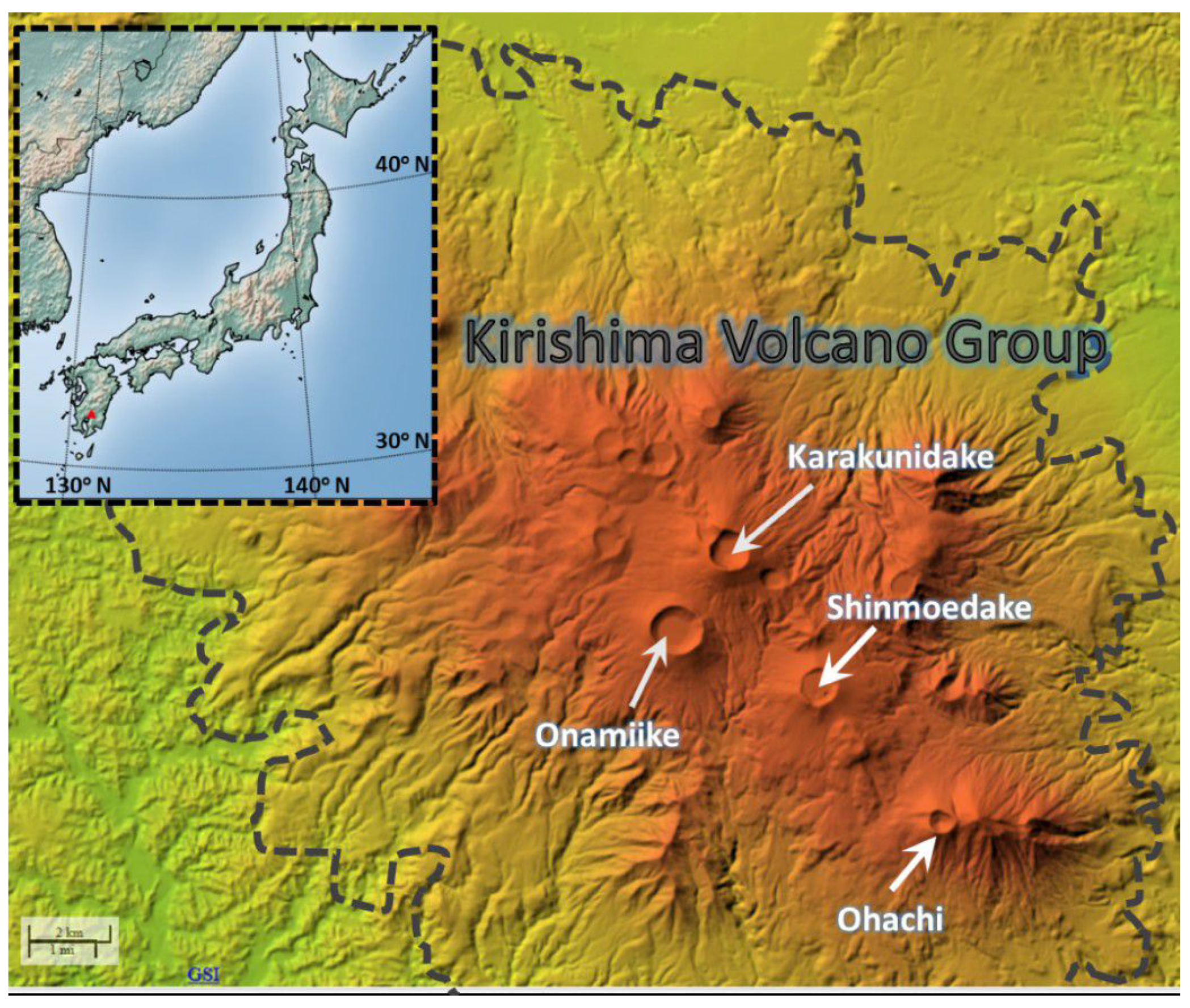
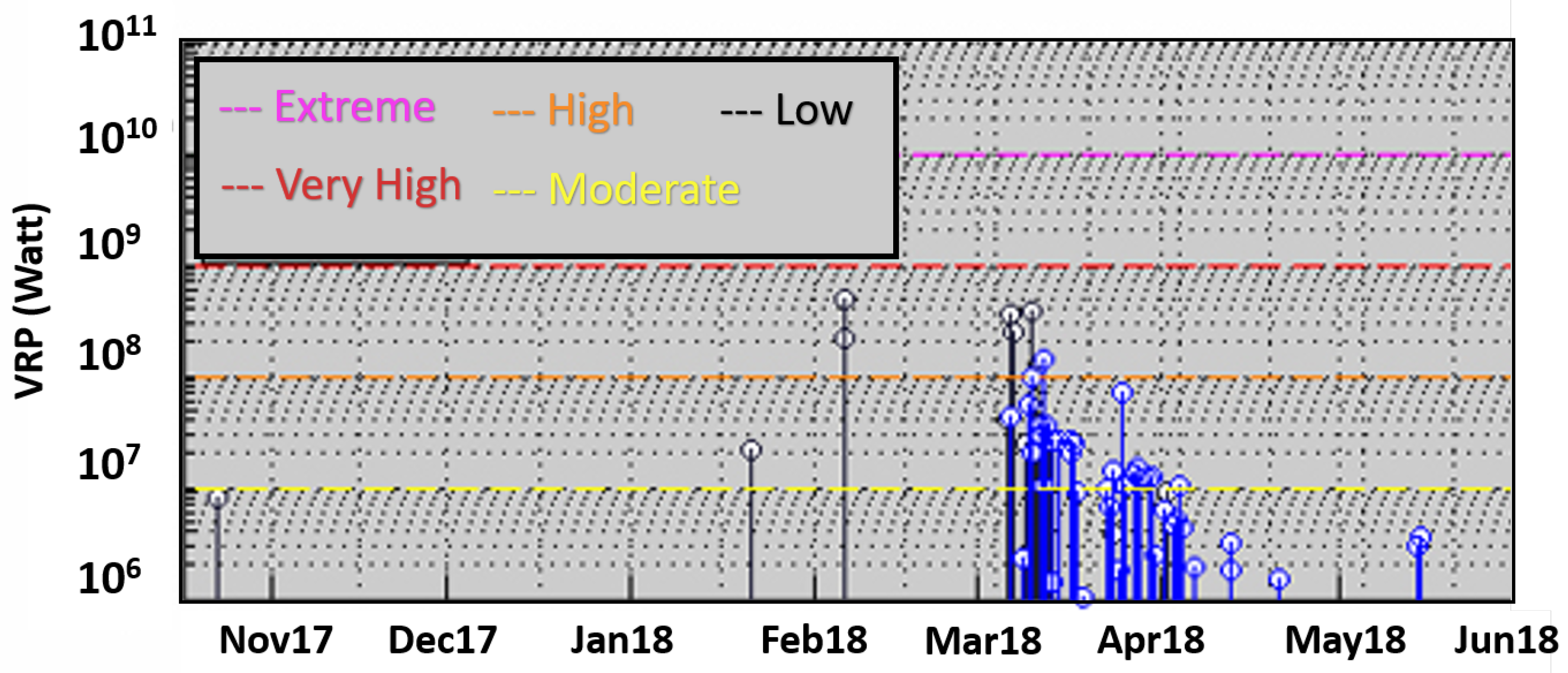
5. Activity at Mt. Shinmoedake in March, 2018

Mount Shinmoedake (elevation ∼1421 m), is a stratovolcano located in southwest Kyushu Island (31°34${}^{\prime }$46.33${}^{″}$N, 130°39${}^{\prime }$29.67${}^{″}$E) and is part of a cluster of volcanoes around Mt. Kirishima (red triangle in Figure 2).

Mount Shinmoedake is one of the currently active volcanoes in Japan. According to a report from the Japan Meteorological Agency (JMA), [32], volcanic activity suddenly recommenced at the beginning of March 2018, and persisted through to April 2018. Violent eruptions ejected ballistic projectiles and the resulting ash plume was blown away from the crater. Figure 3 shows an automated analysis of Moderate Resolution Imaging Spectroradiometer (MODIS) data distributed by the LANCE-MODIS data system and published on the Middle InfraRed Observation of Volcanic Activity (MIROVA) website [33]. The figure showing the thermal anomalies as the volcanic radiative power (VRP) in logarithmic scale, recorded at Mt. Shinmoedake volcano in 2018, clearly shows the sudden intense activity from early March to early April with the category of power intensity in range between moderate and very high, followed by isolated events in May and June 2018. The highest peak appeared and occurred on the 9th and 10th, where the eruption particularly produced the most significant air vibration. We also evaluated infrasound data recorded by the JMA during the major eruptions of the volcano at the start time shown in

Table 2. Recorded major eruptions of Mt. Shinmoedake in the period 10–25 March 2018. JST = Japan standard time.

Date of Eruption	Time (JST = UTC + 9)	Date of Eruption	Time (JST = UTC + 9)
9 March 2018	15:58	11 March 2018	04:05
10 March 2018	01:54		07:46
	04:27	12 March 2018	12:45
	10:15	15 March 2018	14:13
	13:32	25 March 2018	07:35
	18:11

.

Original infrasound data on 10 March 2018, at 01:54, 04:27, 10:15, and 18:11 Japan standard time [JST]), are shown in Figure 4. Strong signals and dense vibrations from the individual eruptions were recorded at stations KUT07, KUT08, KUT09, and KUT10. At the closest station to the crater (distance = 204.29 km), KUT07, a pressure change was first observed about 625 s after the eruption, with delays of another few seconds at other stations. Signals at the farthest station, KUT16 (342.90 km), showed relatively long arrival times (∼18 min) and similarly dense vibrations to those at stations KUT07, KUT08, KUT09, and KUT10. We also observed other signatures at stations KUT01-KUT05, with small volumes/amplitudes. Figures S1–S6 in the supporting information shows similar profiles for other time periods than those in Table 2. We found that twelve stations with different locations had their own signatures that were likely to have originated from several sources, such as waves from the seashore, referred to as microbaroms [34] and mountain-associated waves [35]. In this study, an attempt was made to minimize these to obtain infrasound data sourced from volcanic eruptions.

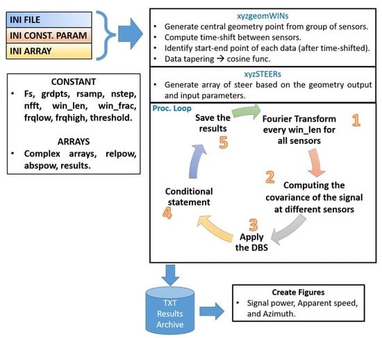
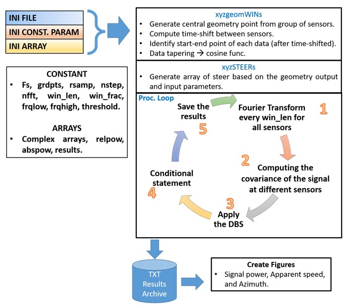
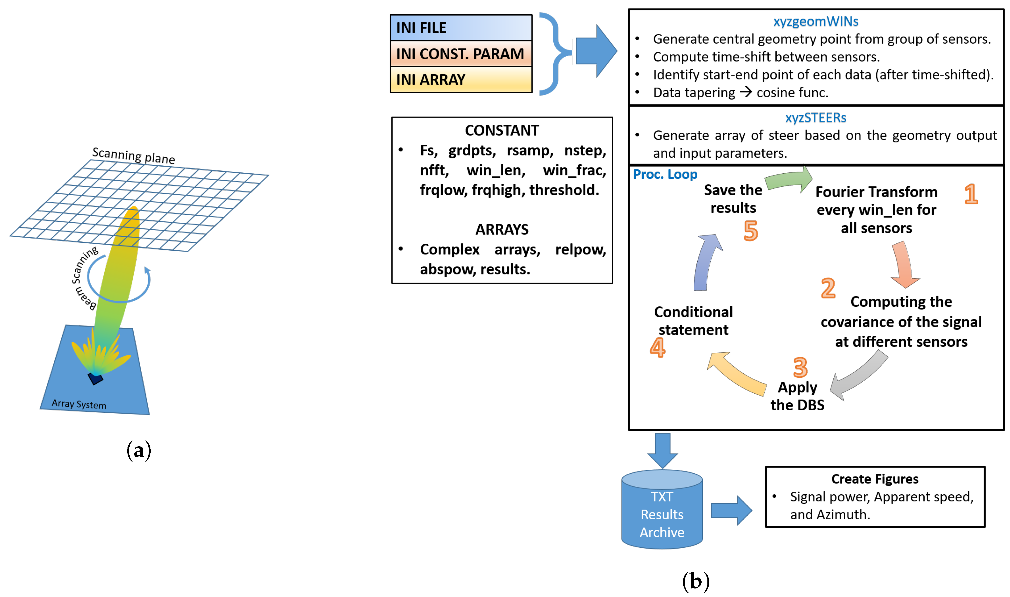
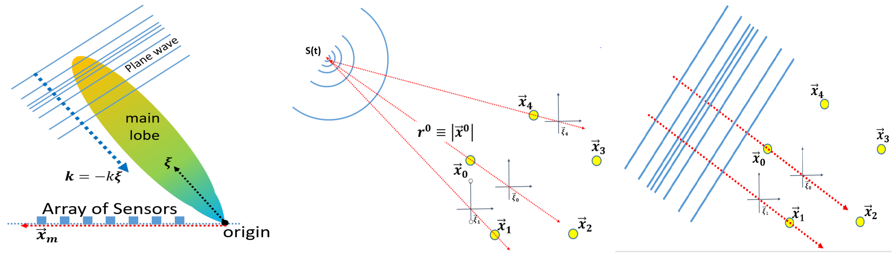
6. Basic Methodology

The basic idea of our approach was to use the set of delays between signals to detect the suspected source waves by steering the array beam to different directions or points in a horizontal scanning region (see Figure 5a).

For our analysis, there were two main data processing steps. Firstly, we evaluated the ambient noise at each individual station to estimate the occurrence probability for each frequency bin of the recorded signals. In this step, we parsed the continuous time series for each station into segments (1-h time series) that overlapped by 50% and distributed them continuously throughout the day. This overlapping reduced the variance in power spectral density (PSD) estimates. The PSD processing computed repeating fast-Fourier transforms (FFT) for each of the separate overlapping time bins of the 1-h time series. The final PSD estimates for the 1-h data were then calculated as the 5th and 95th percentiles of the distribution of individual PSD curves. Plots of the PSDs for our entire period of interest were generated from all individual stations and used for analysis and data quality control.

Secondly, we determined output parameters from irregular array signal processing, such as angle of arrival (azimuth), signal power, the apparent speed, and correlation index. Figure 5b shows schematics that illustrate the processes undertaken in this step. In more detail, at the beginning, several constants and parameters are initialized beside the recorded files. Then, it comes into the main process that split in three sub-processes as follows: (1) The 1st sub-process is called “xyzgeomWINs”, where four actions are executed firstly; (2) the process moves to the 2nd part, named “xyzSTEERs”, which generates a steering array based on the delays between observed signals; and (3) the level of signal coherency between sensors was evaluated for all windowed data at every time shift increment. During this process, rotation scanning to a specific point, based on the calculated time lag between the multiple sensors and a cosine-tapered window function of a certain period length, with the time overlap as a data discontinuity reducer, was applied in the source detection scheme. The window length was chosen to be proportional to the envelope width of the recorded signals. This process continued until the end of the observation data time was reached, and parameters, such as the azimuth angle, signal strength, apparent velocity, and correlation index, were obtained.

To estimate the atmospheric layer where the signal was deflected or refracted down toward the sensor on the Earth, infrasound wave propagation modeling was applied. The propagation modeling used in this study was an approximation of the planar parabolic equation (PE) method [36], with a nonlinear ray tracing model as an addition of the method to draw propagation paths and estimate the arrival time in a three-dimensional inhomogeneous moving medium and the atmospheric background [37]. This method is used to estimate the power loss of a wave transmission as a function of range and altitude. The simulation was run to examine a frequency of 1.25 Hz out to 500 km for the sequence of eruptions listed in Table 2. The frequency range is chosen in order to eliminate the frequency of the interference signals, such as microbarom signals, at around 0.2 Hz and the other mountain wave signals at around 0.7 Hz. The frequency of 1.25 Hz is the center of our band pass filter (1.0–1.5 Hz). This 1.25 Hz frequency is chosen to avoid the remaining harmonic of those interference signals. For the atmospheric absorption of sound, the method used the parameters from Reference [38], which works well even in the upper atmosphere up to 160 km. The simulation also assumed a ground boundary condition as a perfect reflector (rigid plane and no topography).

For a typical source, as listed in Table 2, the sound level at the receiver position depends on the ground conditions, barriers, and meteorological conditions between the source and receiver. In this study, we concentrated on wind effects for sound propagation and ray tracing simulations, assuming the ground surface is perfect reflector without any topography. Therefore, the deviations between the different calculations were caused by parameter variations in the atmospheric profiles. The most important atmospheric effect considered in the study was the refraction caused by wind and vertical atmospheric parameters obtained by the Modern-Era Retrospective analysis for Research and Applications, Version 2 (MERRA-2) and Naval Research Laboratory Mass Spectrometer and Incoherent Scatter Radar, Exosphere (NRLMSISE-00) global atmospheric models. For this study, the 3-h time-averaged horizontal wind, pressure, and temperature fields were accessed via the GMAO web service (Goddard Earth Sciences Data and Information Services Center) [39]. The neutral atmospheric density is retrieved from the model provided by the Community Coordinated Modeling Center [40] in order to complement the atmospheric background conditions in the simulation.

As illustrated in Figure 6, assuming a planar of m-th sensors at locations ${\overrightarrow{x}}_m$ in the xy-plane of our coordinates. The idea of our beam-scanning calculations is quite simple: if a propagating signal is present in an array’s aperture, the sensor outputs are individually weighted and delayed, and then all signals are added together, reinforcing the signal with respect to noise or waves propagating in different directions. The delays that reinforce the signal are directly related to the length of time it takes for the signal to propagate between sensors. In Figure 6, the signal denoted by s(t), traveling from the source at the point ${\overrightarrow{x}}_0$ and an array of all m-th sensors located at $\left\{{\overrightarrow{x}}_m,m=0,\cdots ,M-1\right\}$. The array’s phase center can be defined as the vector quantity $\sum {\overrightarrow{x}}_m$. For simplicity, we choose the origin of our coordinate system to coincide with the phase center, ${\sum }_{m=0}^{M-1}{\overrightarrow{x}}_m=0$. The possible absence of a sensor at the array’s phase center does not preclude using it as the origin and defining all the sensor positions relative to it. The waveform measured by the m-th sensor is $y_m\left(t\right)=f\left({\overrightarrow{x}}_m,t\right)$. The output of our beam-scanning is $z\left(t\right)\equiv {\sum }_{m=0}^{M-1}{w}_m{y}_m\left(t-{\Delta }_m\right)$, where $w_m$ and ${\Delta }_m$ are the amplitude weight and the sensor delay, applying to the output of each sensor. We use the cosine taper function as the amplitude weight to reduce discontinuity between signals. The delays are adjusted to focus the array’s beam on signals propagating in a particular direction ${\overrightarrow{\xi }}_0=-{\overrightarrow{x}}_0/\left|{\overrightarrow{x}}_0\right|$. Similarly, at the m-th sensor, the direction of propagation vector ${\overrightarrow{\xi }}_0$ equals ${\overrightarrow{\xi }}_{0,m}=\left({\overrightarrow{x}}_m-{\overrightarrow{x}}_0\right)/r_{0,m}$, where $r_{0,m}$ is the distance between m-th sensor location and ${\overrightarrow{x}}_0$. In the applications, the origin of the source is undetermined whether the source is located in the near or far field. Thus, for far-field (plane wave) propagation, the vector ${\overrightarrow{\xi }}_0$ does not vary with sensor location, however, for near-field sources, the apparent direction of propagation varies across the array and is thus defined relative to the m-th sensor, ${\overrightarrow{\xi }}_{0,m}$ (see Figure 6). Our case assumes that a far-field source radiates a plane wave having signal s(t) propagates across our array of all m-th sensors in the direction ${\overrightarrow{\xi }}_0$. The waveform within the array’s aperture is given by $f\left(\overrightarrow{x},t\right)=s\left(t-{\overrightarrow{\alpha }}_0·\overrightarrow{x}\right)$, where ${\overrightarrow{\alpha }}_0={\overrightarrow{\xi }}_0/c$ is the slowness vector. At a particular sensor, the waveform is expressed by $y_m\left(t\right)=s\left(t-{\overrightarrow{\alpha }}_0·{\overrightarrow{x}}_m\right)$; the signal output of our beam-scanning becomes $z\left(t\right)={\sum }_{m=0}^{M-1}{w}_{m}s\left(t-{\Delta }_m-{\overrightarrow{\alpha }}_0·{\overrightarrow{x}}_m\right)$. The set of sensor delay is given by ${\Delta }_m=-\overrightarrow{\alpha }·{\overrightarrow{x}}_m=\frac{-\overrightarrow{\xi }·{\overrightarrow{x}}_m}{c}$, thus the output of beam-scanning signal z(t) becomes $z\left(t\right)={\sum }_{m=0}^{M-1}{w}_{m}s\left(t+\left(\overrightarrow{\alpha }-\overrightarrow{{\alpha }_0}\right)·{\overrightarrow{x}}_m\right)$. The output of the velocity vector can be used to calculate the arrival angle of the target, defined by $ta{n}^{-1}\left(\frac{{\alpha }_{0,Y}}{{\alpha }_{0,X}}\right)$, as well as the apparent speed proportional to $\frac{1}{{\overrightarrow{\alpha }}_0}$, where ${\alpha }_{0,X}$ and ${\alpha }_{0,Y}$ are the slowness in the x and y axes, respectively.

For the purposes of computation, we first consider the input to a single sensor at the location ${\overrightarrow{x}}_m$ in terms of a phase shift rather than time delay as $y_m\left(t-{\Delta }_m\right)=y_m\left(t\right)·e^{-i\omega {\Delta }_m}$, where $y_m\left(t\right)=e^{-i\left(\omega t-\overrightarrow{k}·{\overrightarrow{x}}_m\right)}$ and the term of $e^{-i\omega {\Delta }_m}$ represents the phase delay associated with the signal at the m-th sensor, called steering vector e. The beam-scanning output may again be expressed as $z\left(t\right)={\sum }_{m=0}^{M-1}{w}_m·y_m\left(t\right)·e^{-i\omega {\Delta }_m}$. Then, if the phase delay is included in the received signal vector $\overrightarrow{Y}$ $=y_m\left(t\right)·e^{-i\omega {\Delta }_m}$, the term $z\left(t\right)$ in vector notation becomes $\overrightarrow{z}$ = ${\overrightarrow{w}}^H$$\overrightarrow{Y}$, where ${\overrightarrow{w}}^H$ is the weighting vector, and H denotes the complex conjugate transpose. Assuming that the array has already steered to a particular direction, the power of the output signal could be estimated by $P\left(\overrightarrow{z}\right)={\sigma }^2=\mathbb{E}\left\{{\left|\overrightarrow{z}\right|}^2\right\}={\overrightarrow{w}}^H\mathbb{R}\overrightarrow{w}$, where $\mathbb{R}=\mathbb{E}\left\{\overrightarrow{Y}{\overrightarrow{Y}}^H\right\}$ is the correlation matrix of the incoming signal. Using the term of steering vector $\mathit{e}$, the power spectral density of the array output may then be given by using the correlation matrix $\mathbb{R}$ and the steering vector $\overrightarrow{e}$ as $P\left(\overrightarrow{e}\right)={\overrightarrow{e}}^H\mathbb{R}\overrightarrow{e}$. In order to have the beam of our array been unity gain in the output, the power of variance P(z) of the output signal z(t) should be minimized. The solution for optimum weight with respect to this can be given by $\overrightarrow{w}={\displaystyle \frac{{\mathbb{R}}^{-1}\overrightarrow{e}}{\overrightarrow{e}{\mathbb{R}}^{-1}\overrightarrow{e}}}$, and the power becomes ${\displaystyle \frac{1}{{\overrightarrow{e}}^H{\mathbb{R}}^{-1}\overrightarrow{e}}}$.

Finally, we determined the upper wind speed, and then, the direction of the properties of the signal can be recorded. We consider the sound velocity and wind velocity are the function of z and the heterogeneous of the multi-layered Earth’s atmosphere, where each sound ray segment undergoes refraction in such an altitude, which makes the ray becomes more curved and horizontal at its ape; therefore, the trace velocity on the surface is approximately equal to the effective sound speed along its propagating path at the altitude there. This relation may then given by by $c_{tr}^{\prime }=\nu c_{tr}$, where $c_{tr}^{\prime }$, $c_{tr}$, and $\nu$ are referred to as the effective sound speed at an altitude of the reflection, the trace velocity, and the constant factor, i.e., the initial launch angle and atmospheric properties. Trace velocity is constant, along with the ray path, as long as range-independent. In the case of wind case, the trace velocity, using the dispersion relation $\omega =ck$, is given by

$$c_{tr}=\frac{c\left(z\right)}{sin\theta }+w\left(z\right),$$

where $w\left(z\right)$ is the wind velocity at the altitude of z, and $\theta$ is the zenith angle. At the turning $z_{tr}$, the zenith angle is $\theta =\pi /2$; hence, we obtain

$$c_{tr}^{\prime }=c\left(z_{tr}\right)+w\left(z_{tr}\right).$$

7. Results and Discussion

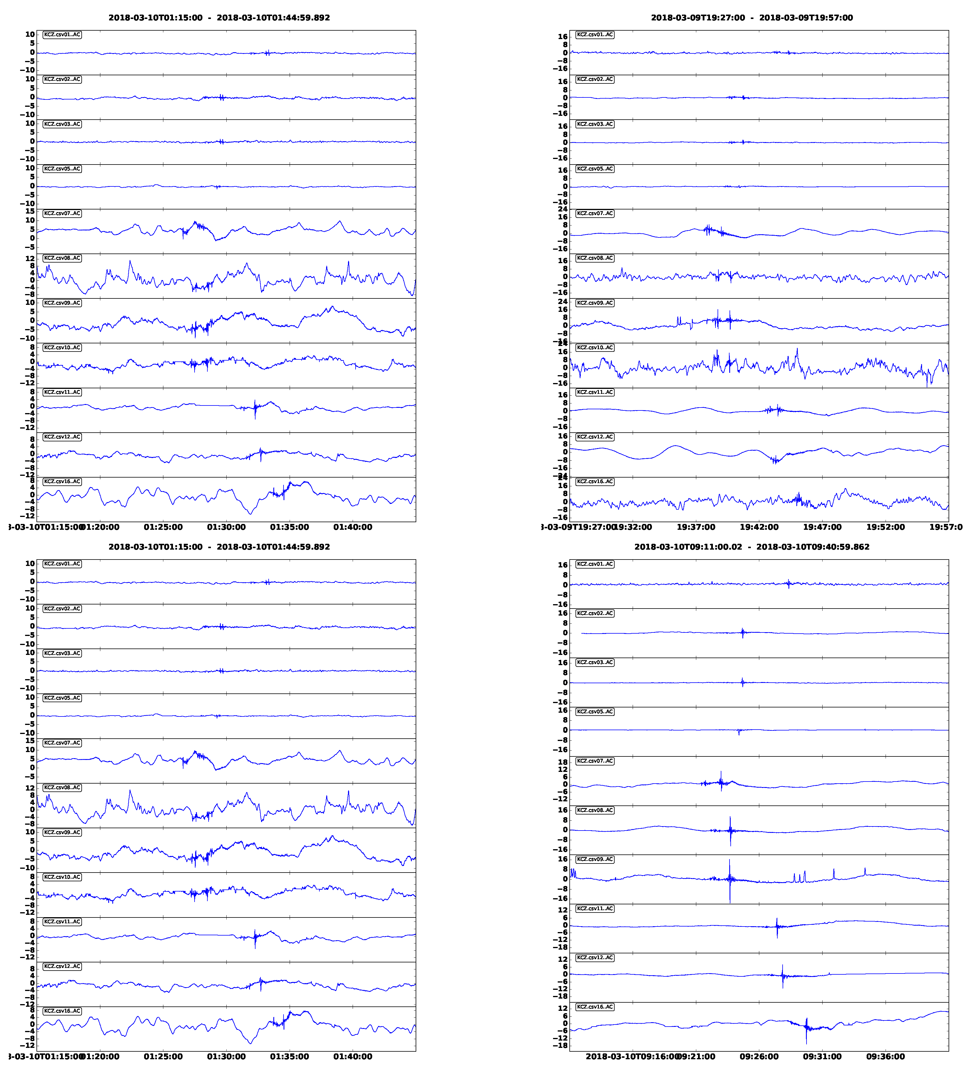
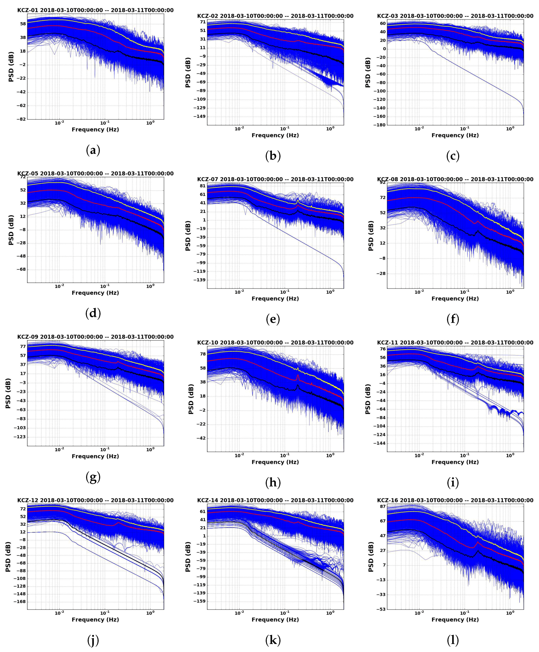
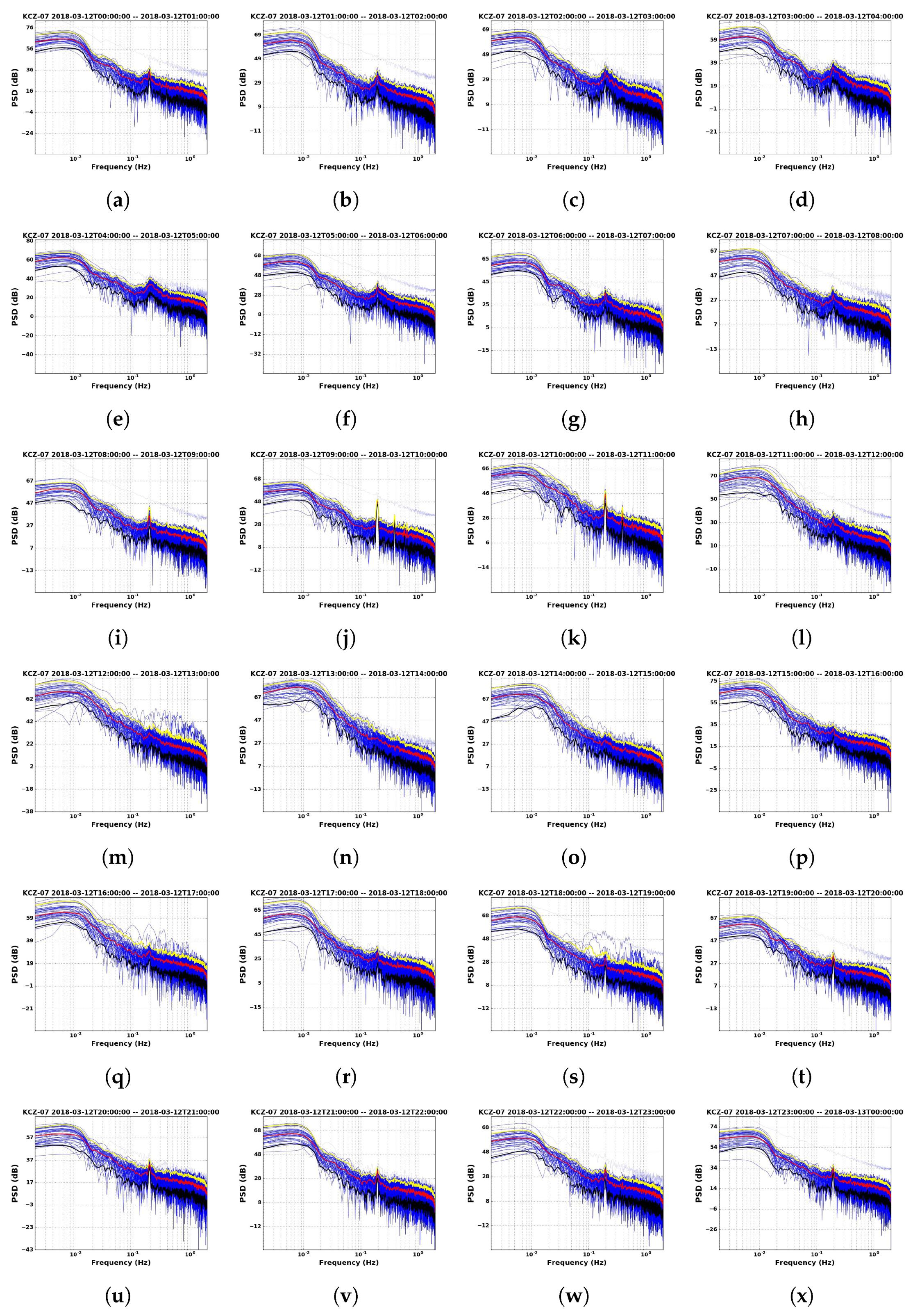
7.1. Coherent Ambient Infrasonic Noise across Stations on Shikoku Island, Japan

Before proceeding to the next analysis steps, which involved filtering signals to reduce noise and the contributions from signals originating from sources that were not of interest, we first applied our method to evaluate the amount of coherent ambient noise for an infrasonic source, using 6–12 h of data at the same times as the eruption events described in Section 5.

It should be noted that all installed sensors are surrounded by mountainous areas, and some of them are close to the ocean. Previous studies investigated mountain-associated infrasound waves by using small arrays of infrasound sensors [41,42]. It was found that the orographically generated infrasonic waves were continuous, with frequencies in the range 0.007–0.1 Hz, and their amplitudes were usually fairly small but occasionally exceeded 1 Pa. The airflow over mountain ranges can generate low-frequency infrasonic waves that can propagate over distances of up to 10–20 km. There is strong evidence that a significant proportion of the events observed in this study were related to wave oscillations at the surface of the ocean (e.g., microbaroms and surf). These ubiquitous waves have frequencies in the range 0.12–0.35 Hz for microbarom sources [34], and 1–20 Hz for sea surf [9]. The microbaroms are also usually characterized by an energy peak between 0.2 and 0.3 Hz in the background infrasound noise and are known to interfere with the detection of explosive events [13] and long-range volcanic eruption signals [43]. As shown in Figure 7, as well as Figures S7–S9 in the supplementary file, the observations at all locations were dominated by these typical airflow signals. More comprehensively, Figure 7 shows an example set of PSD-noise plots for 12 stations on Shikoku Island during a one-day period on 10 March 2018, from consecutive 3-min data segments. PSD for selected stations draw in blue, the 5th and 95th percentiles are plotted in red and black, and the median is in white. Three-min windows and cosine-tapper are used to minimize smoothing of the amplitude distribution in the outer of each data window. All plots of PSD were generated for all stations and used for data quality control and interpretation. Figures S10–S12 in the supplementary file show a set of PSD plots for stations on Shikoku Island for three time periods (e.g., September, November, and December) when the volcano was not in the active phase. Based on all PSDs, the interpretations were as follows. (1) A bit slope spectrum appeared in the data during the time period of the volcanic eruption. These patterns are thought due to the existence of time gaps in the data (Figure 7b,c,e,g,i–k). (2) At stations located on the mountain slope, such as stations KUT05 (Figure 7d), KUT 01 (Figure 7a), and KUT02 (Figure 7b), mountain winds mostly affected the characteristics of the recorded data as infrasonic pressure anomalies. This resulted in the spectral distribution, in the frequency range between 0.01 and 0.1 Hz, undergoing a wide expansion, which depressed the microbarom signals. We noted that the mountain-associated waves were predominantly recorded at the stations in mountainous regions. (3) Signals with a high intensity in the frequency of about 0.2 Hz, commonly called microbaroms, appeared to dominate the recorded data from the stations located close to the ocean (e.g., KUT07 (Figure 7e), KUT08 (Figure 7f), KUT09 (Figure 7g), KUT10 (Figure 7h), KUT14 (Figure 7k), and KUT16 (Figure 7l)). (4) There were monthly seasonal changes in the cumulative signals recorded by each sensor. The total signal recorded during the winter period was more intense than in the opposite season [44,45]. Through global atmosphere circulation, especially in the mid-latitude region, jet stream flows stronger during winter period than the opposite one. (5) Finally, as an addition to the PSD results described above, a comparison was made of the daily background noise among all individual stations. Their variations at infrasound stations were highly variable by season, time of day, and station. Station KUT07 was selected as a sample for the examination of daily PSD variations because it was more responsive to the changes in spectral variations of the received signals. As a result, similar to Bowman’s study, our findings found no significant peak anomalies in the infrasonic noise spectra during noontime (Figure 8). Other similar profiles for other stations during the same time period are shown in Figures S13–S14 in the supplementary file. The dominant frequency found in the PSD profile was then used as the basis for selecting filtered frequencies in our array processing scheme, described in Section 6.

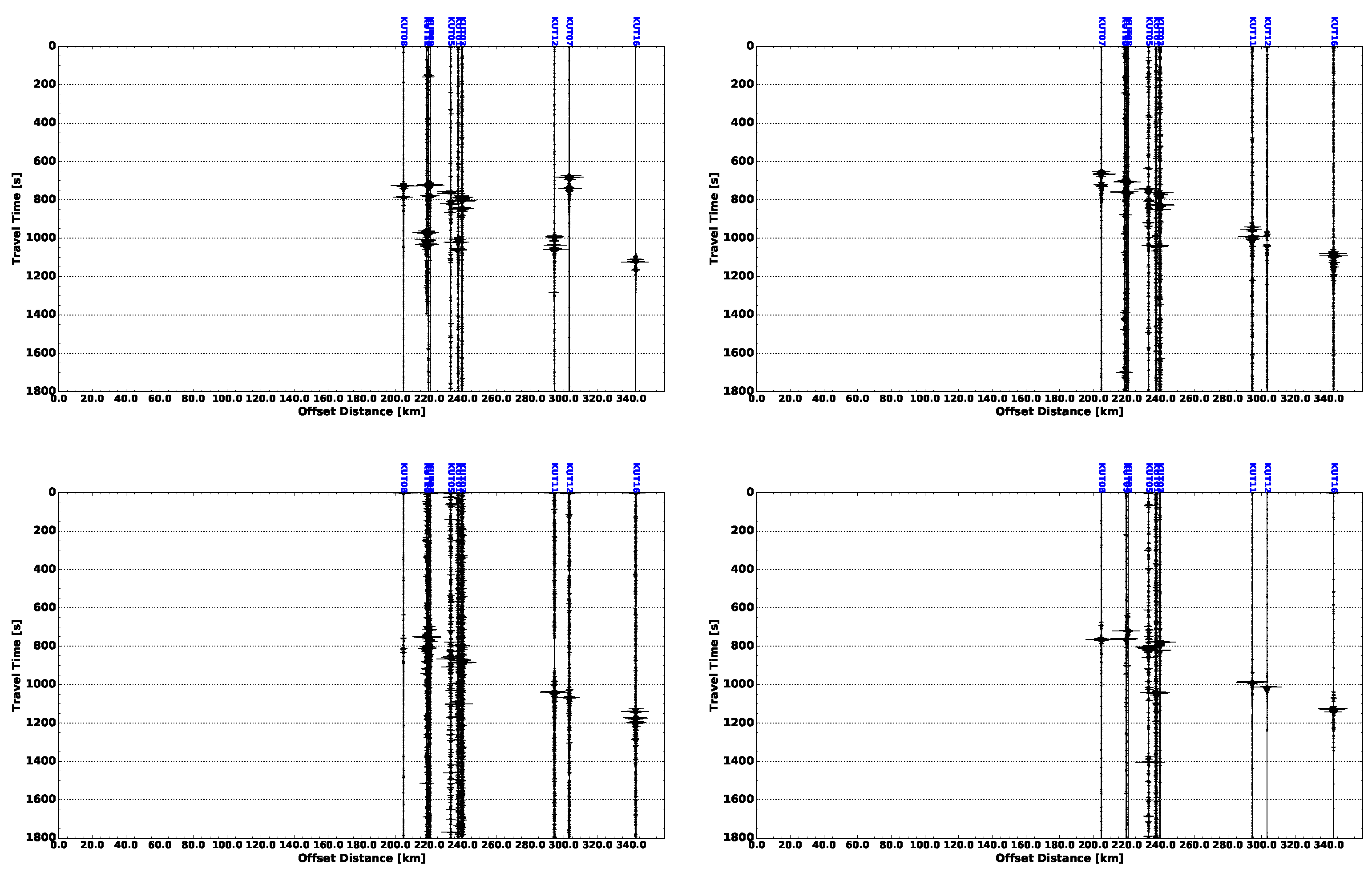
7.2. Infrasound Propagation during the March 2018 Eruptions at Mt. Shinmoedake in Japan

Infrasound generated by explosive eruptions of the volcano was recorded by typical microphones at various distances from the crater. In general, the observed signals traveled across the infrasound stations at near-acoustic wave speeds, indicating that the infrasonic wave fronts propagated a great distance across the Earth’s surface.

In combination with automated processing, the infrasound data provides a basis for more detailed propagation studies assessing wave characteristics. When the location of the source can be associated with a known infrasound source, confidence in estimations of the source localization and propagation speed from the events is high. To illustrate these properties, we focused on data from events described in Section 5, where the origin time determined for each event is shown in Table 2. Each event generates multiple arrival times at different stations, where the times increase as a function of propagation distance (Figure 9). These figures show typical records for the Mt. Shinmoedake eruptions during March, 2018, from stations across Shikoku Island, after bandpass filtering between 1.0 and 1.5 Hz, avoiding the interference signals from the sources described in Section 7.1 (based on Figure 4). Similar plots for the events on 11 and 12 March 2018, are shown in Figures S15 and S16 in the supplementary file. Each figure clearly shows the propagation of the disturbance signature at ∼625 s after the explosion. To estimate the propagation speed of the incoming waves, an envelope of source waves was calculated based on the absolute amplitude of the infrasonic waves recorded at the infrasound stations. In general, four terms could be used to characterize such signals: the beginning, transition, middle, and end periods of the sound wave. To estimate the starting point of each suspected detection, the gradient of the slope at the beginning of the wave envelope was calculated by the elevation angle larger than 45°. Each estimated point corresponds to the position and time of a suspected detection. The gradient of the data for six samples, obtained using numerical linear regression, was used to estimate the propagation speed (see

Table 3. Overall summary of the calculated propagation speeds of the detected signals.

No.	Event Time (JST)	${\mathit{t}}_{\mathit{detection}}$ (after Event Time, s)	$\mathbf{\Delta }$t (s)	Estimated Speed (m/s)
1	0154 on 10 March 2018	657	413	334.18
2	0427 on 10 March 2018	637	398	346.78
3	1015 on 10 March 2018	683	419	329.40
4	1118 on 10 March 2018	625	409	337.45
5	0405 on 11 March 2018	659	406	339.95
6	1245 on 10 March 2018	652	416	331.77

). The propagation speed of the detected signals from the sequence explosive eruption of Mt. Shinmoedake on March 2018 was estimated to be 336.6 ± 6.3 m/s.

Notably, this propagation speed (∼336 m/s) is the speed that the wave travel on the surface from the closest station, sensor number KUT07 to the farthest one, sensor number KUT16. In this case, the sound velocity is about 333 m/s. In a report of Campus in 2006, they estimated a similarly low propagation speed (∼324 m/s) for the 2005 eruption of Lascar volcano in northern Chile, which was recorded by an IMS station about 800 km from the crater [18]. For another event, the 2002 eruption of the Hekla Volcano in the Iceland, Liszka and Garces, in 2002 [14] found that the infrasound propagation speed varied between 315 and 324 m/s. Meanwhile, a higher speed was also detected by an IMS station. The 2005 eruption of Mt. St. Helens generated low-frequency waves traveling at about 352 m/s [18]. The discrepancy between the two eruptions is understandable since the two types of disturbance occurred at different locations.

However, in general, infrasound in the atmosphere propagates at the sound speed of around 340 m/s near the surface/or ground. It is also generally accepted that infrasound propagates at a velocity that typically varies with temperature and the fundamental properties of the propagation medium, as well as the wind velocity [46]. From the above, the speed inferred from our analysis (∼336 m/s) is in the range of typical propagation speeds of infrasonic pressure disturbances from both natural and artificial explosion sources (e.g., chemical and nuclear explosions) [47,48].

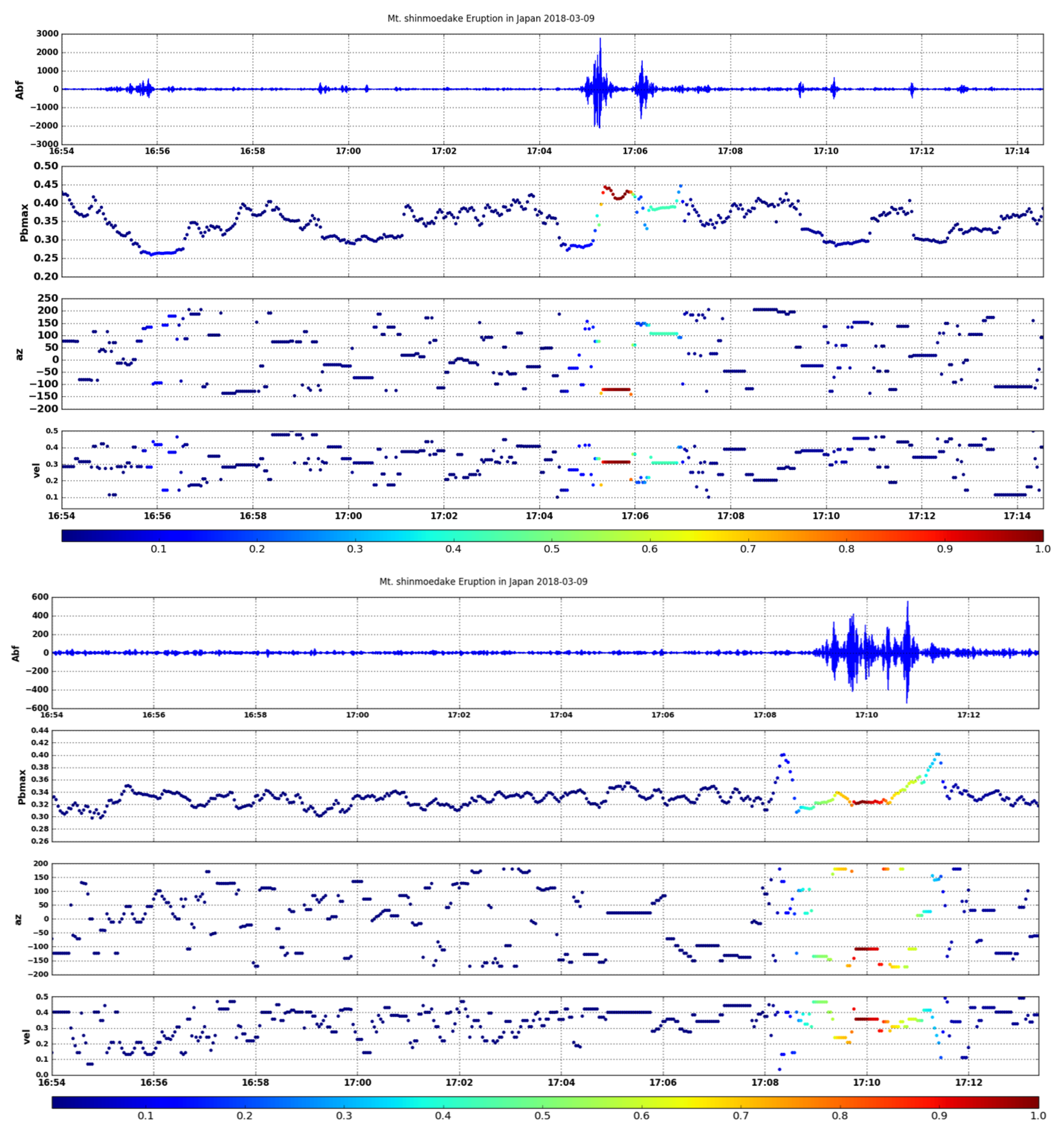
7.3. Infrasound Source Detection

After applying the spectral analysis technique to all infrasound data recorded several hours after the event, it was found that the dataset indicated a peak high spectral density value of around 0.2 Hz, which was the microbarom signal. To avoid this dominant microbarom signal, the frequency range was band-pass filtered with range of 1.0–1.5 Hz. This frequency range was then applied to the filtered data to detect signals in the second process described in Section 6. Figure 10 shows the typical results of the detection process from our calculation, applied to selected station data in the period following the first Mt. Shinmoedake eruption on 9 March 2018, at 06:58 UTC. The figure shows data from four stations located close to the volcano (top panel in Figure 10) and three stations located around 290 km from the source point (bottom panel in Figure 10). From top to bottom, the figure shows the stacked signals received after bandpass filtering, the maximum power at every processing step, the arrival direction as the azimuth angle, and the velocity along the waveform. The color scale indicates the correlation coefficient for the corresponding time window and is a measure of the statistical significance of the source detection. In the recorded data for 9 March 2018, at 06:58 UTC, all of the infrasound data detected by the sensors were propagated at constant speeds, but the estimated azimuths of the incoming signals differed slightly from the actual location of the volcano, which was likely due to the presence of winds and the surface height (i.e., hills), which can cause a signal’s path to stray from the arc of a circle that connects the source to the sensors. A second example is shown in the bottom panel of Figure 10, where the recorded signals were taken from sensors located around 290 km from the infrasound source. In this figure, the signal amplitude is clearly lower amplitude than the result of the upper panel due to many factors, such as topographic absorption and atmospheric conditions. In addition, there was an indication of signals originating from the lower stratosphere within the stable velocity area seen in the velocity panel. A signal phase higher than the sound speed at the ground will be refracted back to the ground along a path where their effective sound speed is approximately equal to the apparent velocity. The apparent speed is calculated based on the sequence signals that is recorded by the sensor at station located close to the source (top panel in Figure 10), indicating the arrival signal as a refraction from the layer at about the troposphere. Meanwhile, the apparent speed in the bottom of Figure 10, showing higher speed than the speed shown in the top panel in Figure 10. Therefore, in the bottom panel in Figure 10, the arrival wave is deducted as a result of refraction at the altitude higher than the troposphere (e.g., stratosphere) due to the flow strength of jet stream on both layers. Generally, jet stream on the stratosphere has a speed higher than on the troposphere. In identifying signal phases and their propagation paths, the celerities, apparent velocities, and back azimuths can be used as a consistency check.

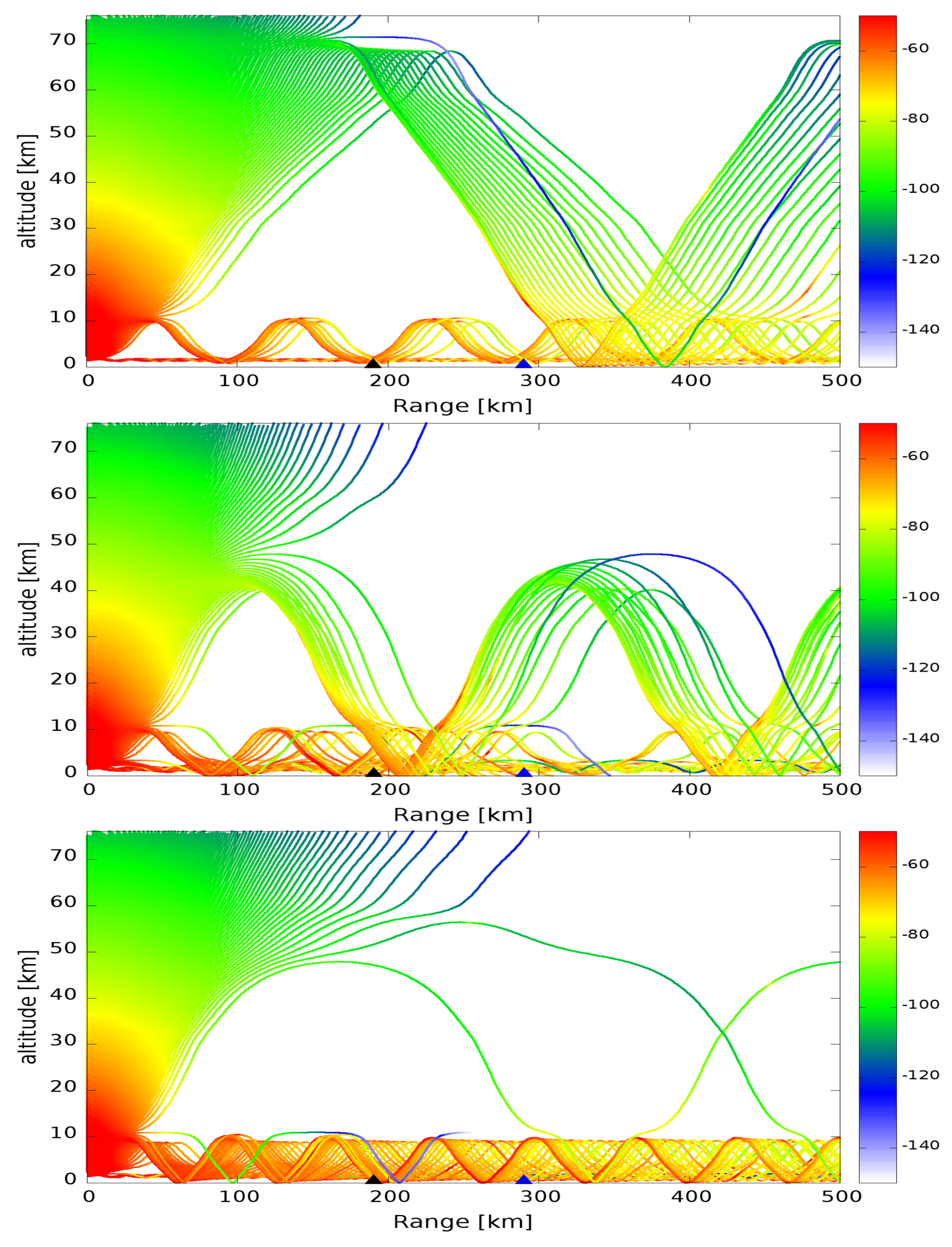
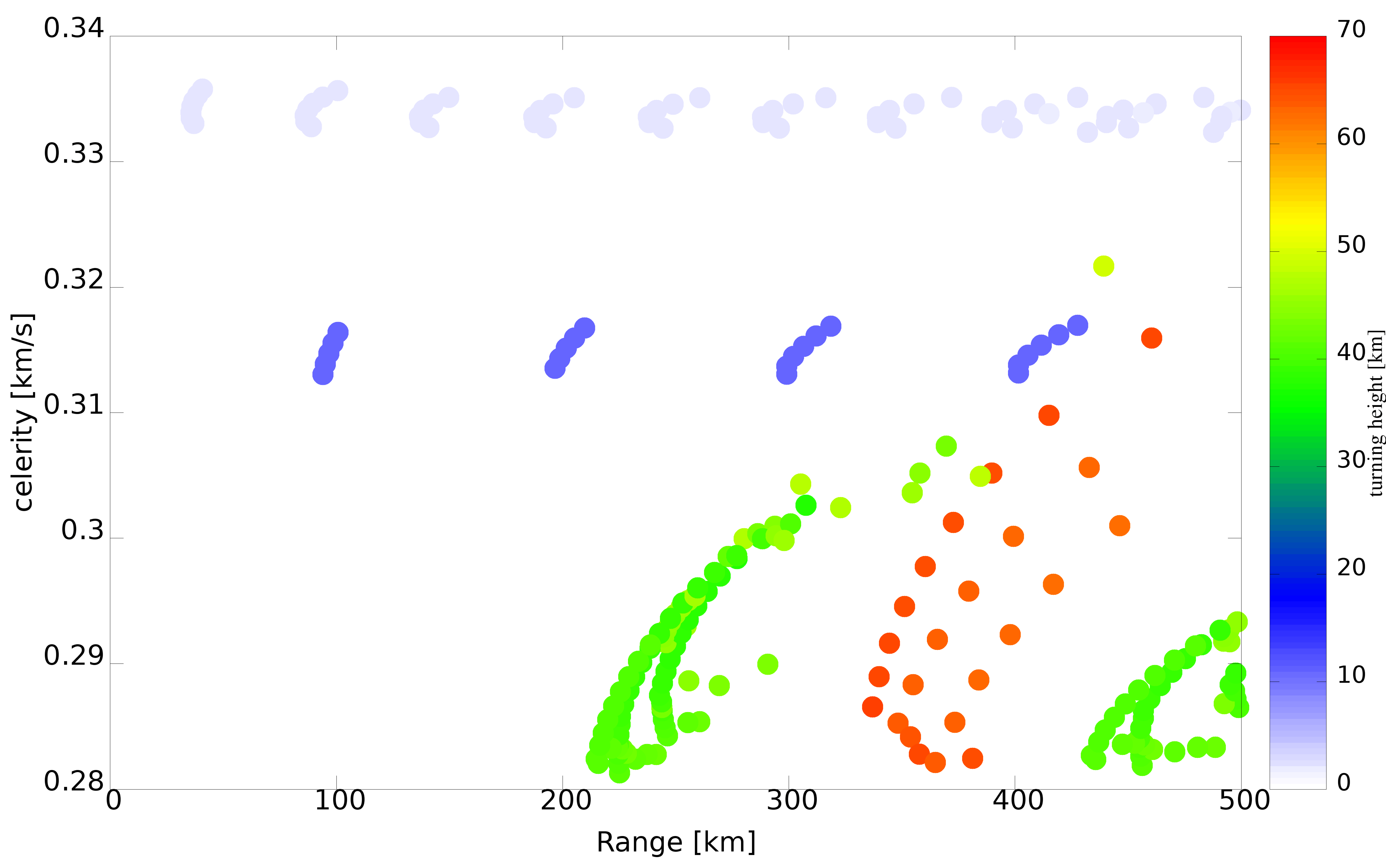
7.4. Infrasound Ray-Propagation

To explain the asymmetry of the location results and to make an infrasound source map, a wave propagation simulation was performed for a broad source area using the planar approximation parabolic equation (PE) method as described in Section 6, and empirical atmospheric data from MERRA-2 and NRLMSISE-00 models were used to predict the power of wave transmission depending on elevation and distance. The resulting MERRA-2 atmospheric specifications provided global estimates of the winds, temperature, and pressure up to 75 km altitude at 3 h intervals and were used in the wave propagation calculations. To account for atmospheric density, available lower and middle atmospheric data were typically provided by the NRLMSISE-00 empirical model.

Figure 11 shows the atmospheric background state above Mt. Shinmoedake on 9 March 2018, at 04:30 UTC. The left panel depicts the eastward and northward winds, denoted by blue and red lines, respectively. Fundamental atmospheric components are shown in the right panel. Long-range sound propagation is primarily determined by horizontal wind components and temperature gradients in terms of altitude, time, and geographic location. Sound is refracted downwards by positive temperature gradients ($\frac{dT}{dz}$> 0), and the sound speed at the refraction layer is larger and equal to the sound speed at the ground, $c\left(z_{tr}\right)\ge c\left(0\right)$ in the windless condition. In the wind case, horizontal wind components, such as positive wind shear, may give play important role in the refraction process. As shown in Figure 11, in the troposphere, temperature decreased up to altitudes below 20 km but, interestingly, a positive temperature gradient occurred twice around altitudes of 5 and 10 km. The layer above this, the stratosphere, was characterized by a strong positive temperature gradient that was predominantly due to the absorption of solar energy in the ozone layer. A smaller layer above it, the stratopause, had a local maximum vertical temperature at an altitude of around 40 to 50 km. In the mesosphere, the temperature decreased dramatically to the minimum state. Obviously, the zonal wind speed was higher than its meridional counterpart in two regions, the altitudes above 10 to 20 km and 30 to 60 km. The maximum value of these jet streams at altitudes near the stratopause and tropopause may have contributed to a ducting layer that refracted sound propagation in a downward direction. Furthermore, during the event, the winds were characterized by a moderately strong eastward zonal wind jet, peaking at ∼40, ∼44, and ∼57 m/s at altitudes of 10, 55, and 68 km, respectively. The meridional winds were greatest at an altitude of 40–60 km. Both the zonal and meridional components of the tropospheric winds had a positive direction, triggering a tropospheric jet to the northeast. For propagation to the north, the sound was predicted to be ducted in the stratosphere, beginning at an altitude of ∼60 km. The main features of the wind specification in the period of 9 March 2018, at 04:30 UTC were a dominance of strong eastward and northward jet streams, peaking at ∼60 and ∼10 km for the stratospheric and tropospheric jets, respectively.

The effective sound speed profiles for propagation to the east predominantly reflected these two wind jets, with great tropospheric and stratospheric ducting predicted for the selected event beginning at altitude ∼10 and ∼60 km. In Figure 12, the along-path wind speed is represented by the difference between the adiabatic (blue line) and effective sound speed (red line) in all directions of wave propagation. It is clearly shown that the westerly wind has a significant impact by completing the formation of the tropo-stratopause sound duct. There was no sound ducting predicted for the west and south propagation, but there was significant tropo-stratospheric ducting for the north and east propagation. Additionally, in this case, the jet stream was large enough to have a qualitative impact on the effective sound speed profiles.

By incorporating the calculated horizontal wind components and vertical atmospheric parameters from the models (see Figure 11), upper altitude reflections of infrasound sources from the north to the east were obtained, as shown in Figure 12. According to the classical ray theory, strong arrivals (totally ducted) were refracted from altitudes for which the effective sound speed was larger than the adiabatic sound speed at the source level (purple shaded color). Figure 12 shows that, for northern propagation, the ducting layer was formed at altitudes above 60 km, although the effective speed of sound at the height of 10 km (see Figure 12) appeared to be greater than the adiabatic sound speed and was a possible candidate for the ducting process; however, the index of the sound speed ratio was not sufficient to form a ducting layer due to the weak meridional component at this height. In the east and northeast propagation, shown in Figure 12, infrasound waves were refracted back to the ground by two different layers, at 40 and 10 km (for eastward propagation) and above 45 and 10 km (for northeast propagation). The eastward and northeastward propagations had three dominant sound speed ratios, which occurred at altitudes around 10 and 40 km. Both profiles had the same index ratio at an altitude of 10 km, but at altitudes above 40 km, they began to show different behaviors in each direction of propagation. For the eastward direction in Figure 13, in addition to being deflected at an altitude of 10 km, the infrasound wave was guided back to the ground at an altitude of 40 km and less of the wave energy propagated to the higher altitude. This was presumably because the index of the two sound speed ratios at an altitude of 40 km in the profile of eastward propagation was significant enough to produce a ducting layer that could guide the wave back to the ground. Infrasound wave energy could possibly have a bias for the upper layer when the index of the two sound speed ratios at a lower altitude was not sufficient to trigger the ducting process, as seen in the east and northeastward propagation profile and clearly in the relationship shown in Figure 12 for similar propagation directions.

The wind jet streams that flowed eastward during the event were significantly larger than those that flowed in the opposite direction. The jet stream produced large tropospheric channels to the east and northeast at an altitude of about 10 km, and in the stratosphere at an altitude of ∼40 to 60 km. At the stations used in this study, which were located northeast of the source location, some tropospheric and stratospheric arrivals were recorded. Based on Figure 9, as well as Figures S12 and S13 in the supplementary file, two examples of station groups were selected, with the results shown in Figure 10. The first and second groups of stations were each about 190 and 290 km from the source location (marked by the black and blue triangles in Figure 13). In addition, at our selected stations, which were located at a distance of about 190 km northeast from the source, only the arrival of the tropospheric north-east propagation was estimated throughout the day, mainly due to the strong wind jet flow around the troposphere and a negative inversion in the boundary layer, with a positive temperature gradient. For the second station group (marked by blue triangles), the two northeast propagation arrivals from the troposphere and stratosphere were estimated throughout the day, because of the presence of the two jet streams in those layers.

In the case of the Mt. Shinmoedake explosion on 9 March 2018, the rays intersecting an area of radius ∼500 km, centered on the source point (marked by the red triangle), were selected to construct a power transmission map (Figure 14). The color code shows the intensity of the power strength at the arrival of the infrasound for each area of the grid. This figure shows the effect of the wind jet corresponding to the background condition of the vertical atmosphere above the source, with the blue colors indicating higher observed amplitudes. As expected, waves propagated over a large area to the northeast of the volcanic region as a potential infrasound source, thus defining a large possible source area. At the time of the eruption, the strong zonal wind blowing toward the northeast would limit the detection of sources west of the volcano. The intensity of the partial strength (blue) repeated itself in concentric bands, resulting from some dominant deflection to the ground. Fortunately, several infrasonic stations detected signature signals from volcanic eruptions, with two phases arriving from the stratosphere and troposphere. The arrival of tropospheric infrasonic waves dominated the signal reception in the first station group, while the stratospheric arrivals were received at the second station group. In addition, the attenuation was very high, with a high absorption power estimated to the south and west after ∼300 km from the source point. In other situations, although the northeast propagation generally dominated, a small number of our sensors in the eastern part of Shikoku Island detected the event.

The various phases of an infrasonic arrival observed by sensors on the ground are determined by the type of propagation path. The paths are predominantly through the tropospheric, stratospheric, and thermospheric waveguides, and depend on their travel times. A wave quantity called celerity can be used to infer the properties of the signal phase. The celerity is defined as the ratio of the range to travel time for one or several multipath bounces and is a measure of the horizontal propagation speed and the path length. Consequently, the closer the propagation path to the horizontal, the closer the speed is to the speed of sound on the ground. Signals that travel along the troposphere obviously arrive first, with celerities close to the speed of sound at the ground. Above the troposphere, stratospheric arrivals have smaller celerities, usually ranging from 0.28 and 0.31 km/s [49]. Finally, the predicted turning height as a function of range and celerity was determined to infer the signal phase properties and propagation paths. We presented a typical example of the analysis of data from the Mt. Shinmoedake eruption period on 9 March 2018, at 06:58 UTC, which enabled a detailed study of sound propagation over time. From classical ray theory, we inferred that the waveguide would be fully channeled if the effective sound velocity at a certain height was relatively large against the sound speed at the ground. The results were shown as the turning height, with the function of celerity and range shown in Figure 15. Typically, three types of arrival were estimated. The first type of arrivals, were called boundary arrivals and were turned back at a height around ∼5 km, with a celerity range of between 0.33 and 0.34 km/s. The second type turned back at altitudes around ∼10–20 km, with an estimated celerity around 0.31 km/s. Along the stratospheric path, there was a double turning height at the same range of celerity of about 0.28 to 0.30 km/s. It was clearly shown that the presence of a strong horizontal wind flow at altitude could alter the length of time required to travel through their path. This effect is shown as a slope pattern in each turning height.

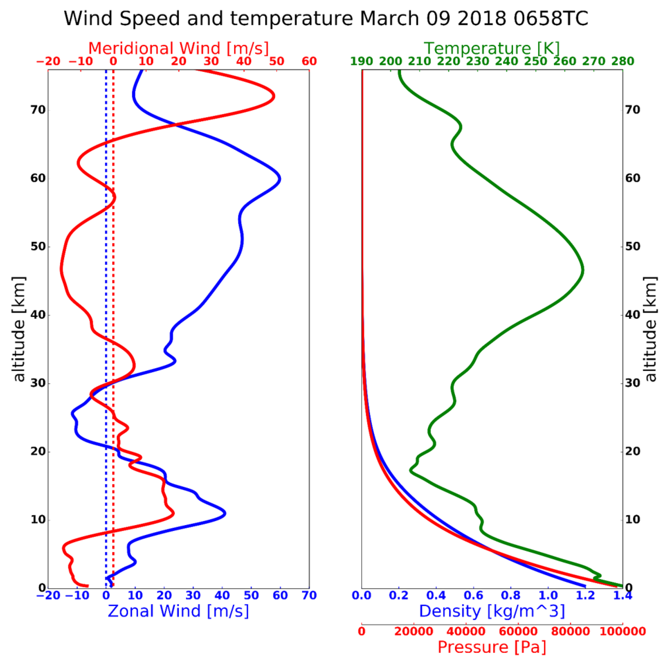
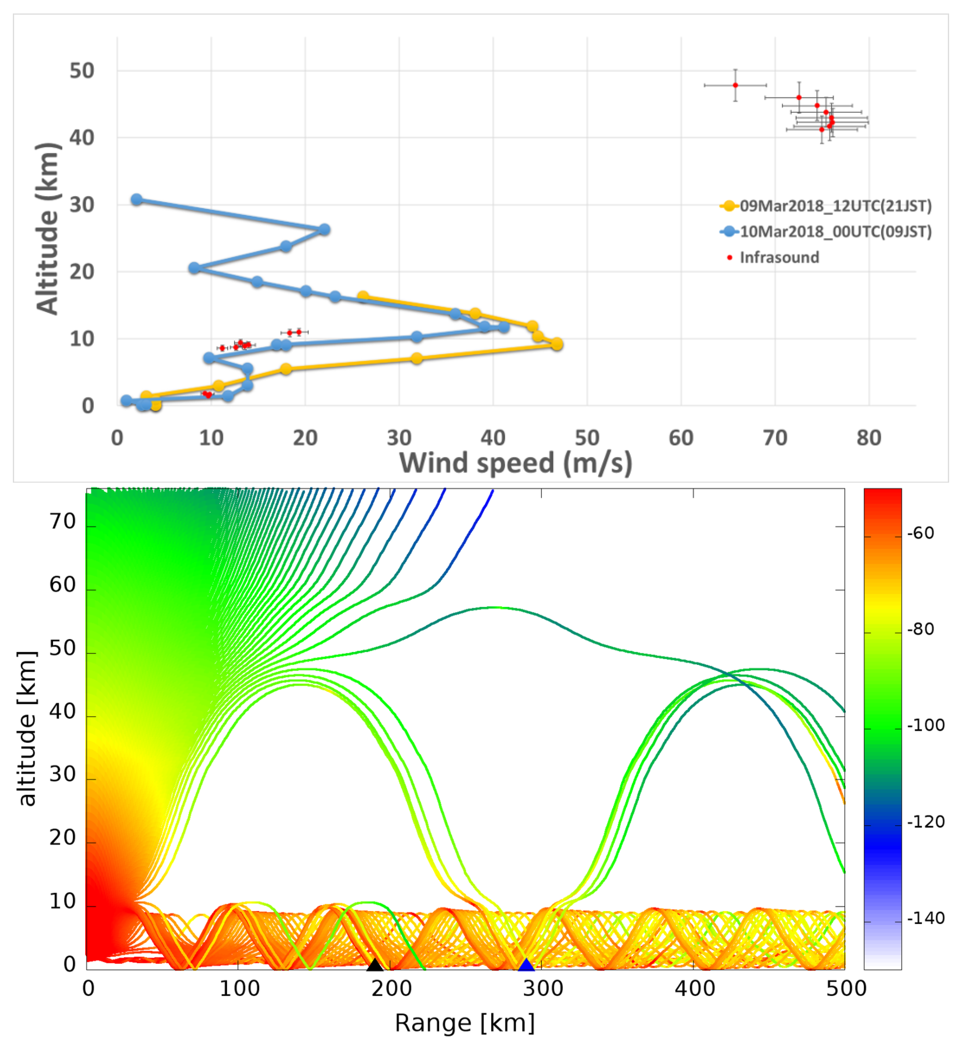
7.5. Comparison of Wind Speed

Two dubiety were found in the approach of atmospheric wind estimation, and one was the exact turning altitude to be estimated and the temperature at this altitude to also be obtained. The altitude level of reflection was estimated by the procedure described in Reference [44] and implemented in the acoustic ray tracing model [36], including the possibility of atmospheric wind, and three fundamental atmospheric profiles, retrieved from MERRA-2 and NRLMSISE-00 models for corresponding time periods above the source location. By applying the initial winds and temperature during the events into the acoustic ray tracing model, the level of infrasonic reflection in a real azimuth propagation from the source are obtained as given in the ray plot (Figure 16, bottom). Rays are plotted at 1° intervals of incidence angles. The stratospheric reflection at about 46 km as a result of the stratospheric jet stream at that time. The rays with lower angles of incidence were not reflected back to the ground which is probably due to the dissipation effects that attenuate the signal.

Figure 17 shows a typical result of radiosonde observation on 9 March 2018 at 00:00 UTC and 12:00 UTC above Shinomisaki station, Japan (33.45°N, 135.77°E). The observation data can be accessed from the JMA database [50] and NOAA (National Oceanic and Atmospheric Administration) [51]. The jet stream in the troposphere, around 10 km of altitude flows strongly in the northeast direction as similar as the MERRA-2 model shown in Figure 11.

Using the result on 9 March 2018 at 06:58 UTC as an example, the sound speed at an altitude of about 40 km was rather low ( 299 m/s at 41 km,

Table 4. Trace velocity, sound speed, and wind speed.

Trace Velocity (km/s)	Computed Reflection Level (km)	Speed of Sound at Reflecting Level (km/s)	Computed wind at Reflecting Level (m/s)
0.3350	1.4399	0.3253	9.7222
0.3350	1.5166	0.3253	9.7253
0.3350	1.5961	0.3252	9.8042
0.3350	1.6845	0.3252	9.8399
0.3350	1.8324	0.3256	9.3737
0.3350	9.5787	0.3238	11.2130
0.3350	9.7079	0.3223	12.6592
0.3350	9.8632	0.3214	13.5737
0.3350	10.0666	0.3210	13.9832
0.3350	10.3885	0.3219	13.1369
0.3350	10.8367	0.3166	18.3671
0.3350	10.9657	0.3157	19.3458
0.3732	41.1735	0.2982	74.9928
0.3732	41.6614	0.2974	75.8096
0.3732	42.2479	0.2971	76.1437
0.3732	42.9495	0.2972	76.0207
0.3732	43.7830	0.2978	75.4465
0.3732	44.7582	0.2987	74.4873
0.3732	45.9465	0.3006	72.5645
0.3732	47.7888	0.3074	65.7910

), indicating the propagation velocity in this layer. Array processing estimated a trace velocity in the propagation direction toward the sensors, with a particular azimuth and speed. As the estimation of trace velocity, based on the recorded signals in this period, was about 375 m/s, the wind over our station at about 41 km was about 76 m/s. In the troposphere, the east wind speeds above our stations at altitudes of 9 and 10 km were about 51 and 53 m/s, respectively. Wind velocity results for this period are shown in the right column of Table 4. The strong wind jets controlled the observed arrivals and further illustrated the importance of the zonal wind jet on propagation simulation. The atmospheric specifications up to the lower stratosphere were sufficient for qualitative propagation simulations. The ray tracing and parabolic modeling of the array are shown in the bottom of Figure 16. Ray tracing predicted the arrival phase of the troposphere at the closest station to the source, labeled as a black triangle, and the arrival phase of the stratosphere at the other station, labeled as a blue triangle, with the sound speed and reflection level given in Table 4.

Typical velocity results for the recorded signals on 9 March 2018 at 06:58 UTC and a comparison with the radiosonde data from local observation at height up to 30 km are presented in Figure 16. A comparison of the calculated wind velocities and radiosonde observation up to the altitude of the radiosonde indicated a qualitative agreement. However, there is still a need to obtain calculated wind velocities above the radiosonde altitude for a comparison with direct measurements (e.g., a stratospheric balloon experiment). The other calculated wind velocities and their comparisons for the the eruption times listed in Table 2 are shown in Tables S3–S7 of the supplementary file.

8. Conclusions

We conducted an analysis of infrasonic data regarding the suspected signatures of an infrasonic pressure disturbance, which was likely to have been caused by an explosive eruption of Mt. Shinmoedake in Japan during the time period listed in Table 2. Specifically, we evaluated individual infrasound data from various stations to identify the characteristics of a particular wave, mostly in terms of its strength, arrival angle, and propagation speed.

Using data from an infrasonic sensor located on Shikoku Island, we then concluded that the propagation speed of the infrasound disturbance associated with the eruption was 336.6 ± 6.3 m/s. The propagation speed was calculated based on the distance between the sensor and the crater, and the delay time between each eruption event and the time of the first detection of the disturbance observed at each infrasonic station. The calculated propagation velocities of around 336 m/s were within the typical range of propagation speeds for similar eruptions [18], which have been observed and analyzed previously. They were also in general agreement with the effective speed of propagation of sound waves [1].

The implementation of the RBS concept into an irregular infrasound array system gives a possible way to detect the source waves, in which the parameter output of the detected source waves are then used for further atmospheric wind velocity estimation. The comparison of the atmospheric wind speed between the infrasound observation and the regional radiosonde observation are relatively in good agreement, although the wind at above the radiosonde altitude still remains works for validations and comparisons through a further improvement of approaches. A knowledge of the trace velocity at these reflection levels would, therefore, be sufficient to calculate the wind speed at the reflection altitudes, giving results that were consistent with direct observations.

The simulation of wave propagation for the Mt. Shinmoedake eruption on 9 March 2018 predicted a map of the distribution of high amplitude arrivals in the northeast direction from the source point. The atmospheric profile in the upper stratosphere was sufficient for qualitative simulations. The strong wind jets further indicated the importance of horizontal wind in the detection and propagation of source waves. Unobserved upper atmospheric arrivals to the sensor arrays were likely in the locations that were still in the range of the shadow zone. However, the arrays did record valuable infrasound arrivals where the western and central array clearly recorded signatures that corresponded to well-estimated tropospheric and stratospheric arrivals.

In summary, we developed a relatively low-cost infrasound sensor array with an irregular shape configuration, our data processing technique for the source detection, and the horizontal wind speed estimation. The sensors were capable of detecting a series of anomalous infrasonic pressure disturbances associated with eruptions of Mt. Shinmoedake during March 2018. We develop a novel irregular array processing for the detection of the infrasound source waves using the common radar scanning scheme. We also introduced a novel idea for the horizontal wind speed estimation using the infrasound observation. The wind speed estimated from infrasound observation showed a profile which is close to the profile obtained by radiosonde. However, it still needs some validations for the estimated wind at above the radiosonde altitude. In addition, as the methods and approaches described in this paper are still based on the general assumptions for simplifying the analysis, we recommend the same procedure be tested for other types of infrasound sources, with some additional adaptive parameters in the procedure.

References

1. Drob, D.P.; Picone, J.M.; Garcés, M. Global morphology of infrasound propagation. J. Geophys. Res. Atmos. 2003, 108. [Google Scholar] [CrossRef]
2. Evers, L.; Haak, H. Tracing a meteoric trajectory with infrasound. Geophys. Res. Lett. 2003, 30, 2246. [Google Scholar] [CrossRef]
3. Garces, M.; Caron, P.; Hetzer, C.; Le Pichon, A.; Bass, H.; Drob, D.; Bhattacharyya, J. Deep infrasound radiated by the Sumatra earthquake and tsunami. Eos Trans. Am. Geophys. Union 2005, 86. [Google Scholar] [CrossRef]
4. Johnson, J.B.; Aster, R.C.; Kyle, P.R. Volcanic eruptions observed with infrasound. Geophys. Res. Lett. 2004, 31. [Google Scholar] [CrossRef]
5. Johnson, J. Generation and propagation of infrasonic airwaves from volcanic explosions. J. Volcanol. Geotherm. Res. 2003, 121, 1–14. [Google Scholar] [CrossRef]
6. Gabrielson, T.B. Infrasound. In Encyclopedia of Acoustics; John Wiley, Ltd.: Chichester, UK, 2007; Chapter 33; pp. 367–372. [Google Scholar] [CrossRef]
7. Ichihara, M.; Takeo, M.; Yokoo, A.; Oikawa, J.; Ohminato, T. Monitoring volcanic activity using correlation patterns between infrasound and ground motion. Geophys. Res. Lett. 2012, 39. [Google Scholar] [CrossRef]
8. Matoza, R.S.; Fee, D. Infrasonic component of volcano-seismic eruption tremor. Geophys. Res. Lett. 2014, 41, 1964–1970. [Google Scholar] [CrossRef] [Green Version]
9. Garcés, M.; Hetzer, C.; Merrifield, M.; Willis, M.; Aucan, J. Observations of surf infrasound in Hawaii. Geophys. Res. Lett. 2003, 30. [Google Scholar] [CrossRef]
10. Johnson, J.B.; Lees, J.M.; Yepes, H. Volcanic eruptions, lightning, and a waterfall: Differentiating the menagerie of infrasound in the Ecuadorian jungle. Geophys. Res. Lett. 2006, 33. [Google Scholar] [CrossRef]
11. Ripepe, M.; Coltelli, M.; Privitera, E.; Gresta, S.; Moretti, M.; Piccinini, D. Seismic and infrasonic evidences for an impulsive source of the shallow volcanic tremor at Mt. Etna, Italy. Geophys. Res. Lett. 2001, 28, 1071–1074. [Google Scholar] [CrossRef]
12. Goerke, V.H.; Young, J.M.; Cook, R.K. Infrasonic observations of the May 16, 1963, volcanic explosion on the island of Bali. J. Geophys. Res. 1965, 70, 6017–6022. [Google Scholar] [CrossRef]
13. Evers, L.G.; Haak, H.W. Listening to sounds from an exploding meteor and oceanic waves. Geophys. Res. Lett. 2001, 28, 41–44. [Google Scholar] [CrossRef]
14. Liszka, L.; Garces, M.A. Infrasonic Observations of the Hekla Eruption of February 26, 2000. J. Low Freq. Noise Vib. Act. Control 2002, 21, 1–8. [Google Scholar] [CrossRef] [Green Version]
15. Christie, D.; Kennett, B.; Tarlowski, C. Detection of Regional and Distant Atmospheric Explosions at IMS Infrasound Stations. In Proceedings of the Infrasound Technology Workshop, Kailua-Kona, Hawaii, 12–15 November 2001. [Google Scholar]
16. Campus, P.; Christie, D.R.; Brown, D. Detection of infrasound from the eruption of Manam volcano on January 27, 2005. In Proceedings of the Infrasound Technology Workshop, Tahiti, French Polynesia, 28 November–2 December 2005. [Google Scholar]
17. Evers, L.; Haak, H. The detectability of infrasound in The Netherlands from the Italian volcano Mt. Etna. J. Atmos. Solar-Terr. Phys. 2005, 67, 259–268. [Google Scholar] [CrossRef]
18. Campus, P. Monitoring volcanic eruptions with the IMS infrasound network. Inframatics 2006, 15, 6–12. [Google Scholar]
19. Campus, P. The IMS infrasound network: Detection of a large variety of events including volcanic eruptions. In Proceedings of the 8th International Conference on Theoretical and Computational Acoustics, Crete, Greece, 2–5 July 2007. [Google Scholar]
20. Caudron, C.; Taisne, B.; Garcés, M.; Alexis, L.P.; Mialle, P. On the use of remote infrasound and seismic stations to constrain the eruptive sequence and intensity for the 2014 Kelud eruption. Geophys. Res. Lett. 2015, 42, 6614–6621. [Google Scholar] [CrossRef]
21. Cansi, Y. An automatic seismic event processing for detection and location: The PMCC Method. Geophys. Res. Lett. 1995, 22, 1021–1024. [Google Scholar] [CrossRef]
22. Cansi, Y.; Le Pichon, A. Infrasound Event Detection Using the Progressive Multi-Channel Correlation Algorithm. In Handbook of Signal Processing in Acoustics; Springer: New York, NY, USA, 2009; pp. 1425–1435. [Google Scholar] [CrossRef]
23. Lopez, T.; Fee, D.; Prata, F.; Dehn, J. Characterization and interpretation of volcanic activity at Karymsky Volcano, Kamchatka, Russia, using observations of infrasound, volcanic emissions, and thermal imagery. Geochem. Geophys. Geosyst. 2013, 14, 5106–5127. [Google Scholar] [CrossRef]
24. Marchetti, E.; Ripepe, M.; Ulivieri, G.; Caffo, S.; Privitera, E. Infrasonic evidences for branched conduit dynamics at Mt. Etna volcano, Italy. Geophys. Res. Lett. 2009, 36. [Google Scholar] [CrossRef]
25. Ripepe, M.; De Angelis, S.; Lacanna, G.; Voight, B. Observation of infrasonic and gravity waves at Soufrière Hills Volcano, Montserrat. Geophys. Res. Lett. 2010, 37. [Google Scholar] [CrossRef]
26. Olson, J.V.; Szuberla, C.A. Processing Infrasonic Array Data. In Handbook of Signal Processing in Acoustics; Havelock, D., Kuwano, S., Vorländer, M., Eds.; Springer: New York, NY, USA, 2008; pp. 1487–1496. [Google Scholar] [CrossRef]
27. Cansi, Y.; Klinger, Y. An automated data processing method for mini-arrays. News Lett 1997, 11, 2–4. [Google Scholar]
28. Yamamoto, M.Y.; Yokota, A. Infrasound Monitoring for Disaster Prevention from Geophysical Destructions. In Proceedings of the 5th Internationnl Symposium on Frontier Technology 2015 (ISFT 2015), Kunming, China, 24–28 July 2015. [Google Scholar]
29. SAYA Inc. Infrasound Sensor ADX3I-INF01LE. Multifunction-I/O XIII. Available online: https://www.saya-net.com/products/INF01.html (accessed on 22 February 2020).
30. Kochi University of Technology (KUT). Kochi University of Technology InfraSound Observation Data Monitoring System. Real Time Infrasound Data - KUT. Available online: http://infrasound.kochi-tech.ac.jp/infrasound/graph.php (accessed on 20 January 2019).
31. Space Laboratory of KUT. KUT Infrasound March 2018. Available online: https://figshare.com/articles/KUT_Infrasound_March2018/8319824/1 (accessed on 26 November 2019).
32. Japan Meteorological Agency (JMA). Monthly Volcanic Activity Report; Tokyo, Japan, 2018. Available online: https://www.data.jma.go.jp/svd/vois/data/tokyo/eng/volcano_activity/monthly.htm. (accessed on 26 November 2019).
33. MIROVA. Middle InfraRed Observation of Volcanic Activity - Thermal Anomalies. Available online: http://www.mirovaweb.it/?action=about (accessed on 13 January 2018).
34. Garcés, M.; Willis, M.; Hetzer, C.; Le Pichon, A.; Drob, D. On using ocean swells for continuous infrasonic measurements of winds and temperature in the lower, middle, and upper atmosphere. Geophys. Res. Lett. 2004, 31. [Google Scholar] [CrossRef]
35. Landès, M.; Ceranna, L.; Le Pichon, A.; Matoza, R.S. Localization of microbarom sources using the IMS infrasound network. J. Geophys. Res. Atmos. 2012, 117. [Google Scholar] [CrossRef] [Green Version]
36. Waxler, R.M.; Assink, J.D.; Hetzer, C.; Velea, D. NCPAprop—A software package for infrasound propagation modeling. J. Acoust. Soc. Am. 2017, 141, 3627. [Google Scholar] [CrossRef]
37. Gossard, E.E.; Hooke, W.H. Waves in the atmosphere: Atmospheric infrasound and gravity waves: Their generation and propagation. In Developments in Atmospheric Science 2; Elsevier Scientific: Amsterdam, The Netherlands, 1975; pp. 423–440. [Google Scholar]
38. Sutherland, L.C.; Bass, H.E. Atmospheric absorption in the atmosphere up to 160 km. J. Acoust. Soc. Am. 2004, 115, 1012–1032. [Google Scholar] [CrossRef]
39. Goddard Earth Sciences Data and Information Services Center (GES DISC). Global Modelling and Assimilation Office (GMAO) (2015). Available online: https://disc.gsfc.nasa.gov/datasets/M2T3NVASM_V5.12.4. (accessed on 12 February 2018).
40. Community Coordinated Modeling Center-NASA. NRLMSISE-00 Atmosphere Model 2001. Available online: https://ccmc.gsfc.nasa.gov/modelweb/models/nrlmsise00.php (accessed on 12 February 2018).
41. Wilson, C.R.; Olson, J.V. Mountain associated waves at I53US and I55US in Alaska and Antartica in the frequency passband from 0.015 to 0.10 Hz. Inframatics 2003, 3, 6–10. [Google Scholar]
42. Wilson, C.R.; Szuberla, C.A.L.; Olson, J.V. High-latitude Observations of Infrasound from Alaska and Antarctica: Mountain Associated Waves and Geomagnetic/Auroral Infrasonic Signals. In Infrasound Monitoring for Atmospheric Studies; Le Pichon, A., Blanc, E., Hauchecorne, A., Eds.; Springer: Dordrecht, The Netherlands, 2009; pp. 415–454. [Google Scholar] [CrossRef]
43. Matoza, R.S.; Vergoz, J.; Le Pichon, A.; Ceranna, L.; Green, D.N.; Evers, L.G.; Ripepe, M.; Campus, P.; Liszka, L.; Kvaerna, T.; et al. Long-range acoustic observations of the Eyjafjallajökull eruption, Iceland, April–May 2010. Geophys. Res. Lett. 2011, 38. [Google Scholar] [CrossRef] [Green Version]
44. Donn, W.L.; Rind, D. Natural Infrasound as an Atmospheric Probe. Geophys. J. Int. 1971, 26, 111–133. [Google Scholar] [CrossRef] [Green Version]
45. Donn, W.L.; Rind, D. Microbaroms and the Temperature and Wind of the Upper Atmosphere. J. Atmos. Sci. 1972, 29, 156–172. [Google Scholar] [CrossRef] [Green Version]
46. Evers, L.G.; Haak, H.W. The Characteristics of Infrasound, its Propagation and Some Early History. In Infrasound Monitoring for Atmospheric Studies; Le Pichon, A., Blanc, E., Hauchecorne, A., Eds.; Springer: Dordrecht, The Netherlands, 2009; pp. 3–27. [Google Scholar] [CrossRef]
47. Assink, J.; Averbuch, G.; Shani-Kadmiel, S.; Smets, P.; Evers, L. A Seismo-Acoustic Analysis of the 2017 North Korean Nuclear Test. Seismol. Res. Lett. 2018, 89, 2025–2033. [Google Scholar] [CrossRef] [Green Version]
48. Ceranna, L.; Le Pichon, A.; Green, D.N.; Mialle, P. The Buncefield explosion: A benchmark for infrasound analysis across Central Europe. Geophys. J. Int. 2009, 177, 491–508. [Google Scholar] [CrossRef] [Green Version]
49. Brown, D.J.; Katz, C.N.; Le Bras, R.; Flanagan, M.P.; Wang, J.; Gault, A.K. Infrasonic Signal Detection and Source Location at the Prototype International Data Centre. Pure Appl. Geophys. 2002, 159, 1081–1125. [Google Scholar] [CrossRef]
50. Japan Meteorological Agency (JMA). High-rise Meteorological Observation Database. Available online: https://www.data.jma.go.jp/obd/stats/etrn/upper/ (accessed on 8 July 2019).
51. National Oceanic and Atmospheric Administration (NOAA). NOAA/ESRL Radiosonde Database. Available online: https://ruc.noaa.gov/raobs/ (accessed on 8 July 2019).
Figure 1. The locations of infrasound sensors (type: ADXII-INF01) in Japan. (top) Distribution of sensor location over Japan; (bottom) infrasound sensor location over Shikoku island, Japan.
Remotesensing 12 00728 g001
Figure 2. Topographic map of Mt. Shinmoedake and the Mt. Kirishima volcano cluster. Image is taken from Japan Meteorological Agency (JMA) website.
Remotesensing 12 00728 g002
Figure 3. Log of the radiative power of Mt. Shinmoedake, Japan, during 2018 (table is taken from the Middle InfraRed Observation of Volcanic Activity (MIROVA) website, [33]. The color lines, respectively, describe for extreme level (pink); very high level (red); high level (orange); moderate level (yellow); and low level (black).
Remotesensing 12 00728 g003
Figure 4. Records of infrasonic pressure data for 10 March 2018, at 01:54 Japan standard time (JST) (top-left), 04:27 JST (top-right), 10:15 JST (bottom-left), and 18:11 JST (bottom-right), showing the arrival times of air pressure disturbances for stations on Shikoku Island following the Mt. Shinmoedake eruption on 10 March 2018. The x-axis is the observation time in UTC, and the y-axis is the infrasonic pressure in Pa.
Remotesensing 12 00728 g004
Figure 5. The illustration of the approach used in this study. (a) The idea behind Radar Beam Swinging in steering the beam of the array on a scanning plane to detect a suspected source waves. (b) Schematic illustrating the steps in our approach to determine the arrival direction and propagation speed of the incoming signal’s source.
Remotesensing 12 00728 g005
Figure 6. The phase center of the array is the origin of a coordinate system. x 0 denote as a source location emits a signal s(t) that propagates to the array in a particular direction ξ 0 . The distance between the origin and the source is r x 0 . (Left) Illustration of sensor array, the direction represented by a main lobe and a plane wave incident from direction of the main lobe. (Right) The illustration for far-field propagation, the apparent direction of propagation does not vary with sensor location.
Remotesensing 12 00728 g006
Figure 7. A set of power spectral density (PSD) plots for stationson Shikoku Island during a one-day period on 10 March 2018 (blue). The 5th and 95th percentiles (black and red) and the median (white) for each plot. Figure (al) show the PSD results of the one-day signals recorded by sensor KUT01, KUT02, KUT03, KUT05, KUT07, KUT08, KUT09, KUT10, KUT11, KUT12, KUT14, and KUT16, respectively.
Remotesensing 12 00728 g007
Figure 8. Power spectral density (PSD) for station KUT07 on 12 March 2018 for all time intervals (blue), the 5th and 95th percentiles (yellow and black), and the median (white) value for each time interval. The rows group plots by 1-h time intervals for 4 h. Figure (ax) respectively show the PSD results of the one-hour signals recorded by sensor KUT07.
Remotesensing 12 00728 g008
Figure 9. Records of the Mt. Shinmoedake eruptions on 10 March 2018, at 01:54 JST (top-left), 04:27 JST (top-right), 10:15 JST (bottom-left), and 18:11 JST (bottom-right), from the stations on Shikoku Island. The results are filtered in the frequency range 1.0–1.5 Hz based on the PDF plot shown in Figure 4.
Remotesensing 12 00728 g009
Figure 10. (Top panel) Array processing results for the 9 March 2018 at 06:58 UTC based on the data of the closest station to the source point. Clear arrival with both arrival direction and apparent velocity are presented in stable value. The detection is colored by the coherent coefficient. (Bottom panel) Similar processing on the same period based on the second group of station data.
Remotesensing 12 00728 g010
Figure 11. Modern-Era Retrospective analysis for Research and Applications, Version 2 (MERRA-2) and Naval Research Laboratory Mass Spectrometer and Incoherent Scatter Radar, Exosphere (NRLMSISE-00) atmospheric profiles above the source for use in the wave propagation calculation. (left panel) Winds, with the eastward winds as a blue solid line and northward winds as a blue dotted line. (right panel) Fundamental atmospheric parameters, vertical temperature, density, and pressure shown in green, blue, and red lines.
Remotesensing 12 00728 g011
Figure 12. Effective sound speed comparisons for Modern-Era Retrospective analysis for Research and Applications, Version 2 (MERRA-2) and Naval Research Laboratory Mass Spectrometer and Incoherent Scatter Radar, Exosphere (NRLMSISE-00) model specifications above Mt. Shinmoedake on 9 March 2018, at 04:30 UTC. Purple shading represents the condition when c e f f ≥ c.
Remotesensing 12 00728 g012
Figure 13. Ray tracing plot for the power transmission from Mt. Shinmoedake at 0 km at the left edge of the plot out to 500 km. The plot was constructed using atmospheric data for 9 March 2018, at 04:30 UTC. The top, middle, and bottom figures show the results for the northward, eastward, and northeastward propagation directions, respectively. The color plot represents the sound wave power transmission in dB per km of propagation of the infrasonic wave at a frequency of 1.25 Hz.
Remotesensing 12 00728 g013
Figure 14. Sound wave power maps in dB for 9 March 2018, at 04:30 UTC from the 1.25 Hz propagation modeling. The red triangle is the Mt. Shinmoedake volcano. The color plot represents the sound wave power loss in dB, where the blue is a larger loss than the green.
Remotesensing 12 00728 g014
Figure 15. Celerity-range diagram. The colored dots represent troposphere and stratosphere ducting according to the turning height.
Remotesensing 12 00728 g015
Figure 16. Typical results on 9 March 2018, at 06:58 UTC. (top) Wind velocity obtained by calculation (red dot) and radiosonde observations (blue and yellow circles). (bottom) Typical ray-tracing results for a real azimuth propagation from the source to the array sensor. The colored dots represent troposphere and stratosphere ducting according to the turning height. The colored plot represents sound wave power transmission in dB per kilometer of propagation of the infrasonic wave at a frequency of 1.25 Hz.
Remotesensing 12 00728 g016
Figure 17. A typical result from radiosonde observation above Shinomisaki station, Japan (33.45°N, 135.77°E), on 9 March 2018 at 00 UTC (the first line panel) and 12 UTC (the second line panel). The zonal and the meridional winds are, respectively, drawn in blue and yellow lines.
Remotesensing 12 00728 g017