Performance Assessment of ICESat-2 Laser Altimeter Data for Water-Level Measurement over Lakes and Reservoirs in China

Abstract

Although the Advanced Topographic Laser Altimeter System (ATLAS) onboard the Ice, Cloud, and Land Elevation Satellite-2 (ICESat-2) was primarily designed for glacier and sea-ice measurement, it can also be applied to monitor lake surface height (LSH). However, its performance in monitoring lakes/reservoirs has rarely been assessed. Here, we report an accuracy evaluation of the ICESat-2 laser altimetry data over 30 reservoirs in China using gauge data. To show its characteristics in large-scale lake monitoring, we also applied an advanced radar altimeter SARAL (Satellite for ARgos and ALtika) and the first laser altimeter ICESat (Ice, Cloud and land Elevation Satellite) to investigate all lakes and reservoirs (>10 km²) in China. We found that the ICESat-2 has a greatly improved altimetric capability, and the relative altimetric error was 0.06 m, while the relative altimetric error was 0.25 m for SARAL. Compared with SARAL and ICESat data, ICESat-2 data had the lowest measurement uncertainty (the standard deviation of along-track heights; 0.02 m vs. 0.17 m and 0.07 m), the greatest temporal frequency (3.43 vs. 1.35 and 1.48 times per year), and the second greatest lake coverage (636 vs. 814 and 311 lakes). The precise LSH profiles derived from the ICESat-2 data showed that most lakes (90% of 636 lakes) had a quasi-horizontal LSH profile (measurement uncertainty <0.05 m), and special methods are needed for mountainous lakes or shallow lakes to extract precise LSHs.

1. Introduction

Lakes and reservoirs are highly sensitive to climate change [1,2] and human activities [3]. Monitoring their dynamics from space is important for water management and drought monitoring [4,5,6,7], especially for remote and less developed regions where hydrological data is rare or hard to access [8,9].

Satellite altimetry is an important tool for monitoring lake surface height (LSH) [10,11,12,13], but faces several difficulties in large-scale lake studies. First, there are large spatial gaps between tracks (dozens to hundreds of kilometers) and many lakes are unmonitored. Second, precedent altimeters usually have large temporal gaps, such as the first laser altimeter ICESat (Ice, Cloud, and Land Elevation Satellite) [14,15] which cannot describe the lake seasonality in detail. Third, conventional altimeters usually have large altimetric error in LSH for some small lakes because they usually have a large footprint size (several kilometers), resulting in mixed signals contaminated by the surrounding land (waveform pollution). Therefore, spatial, temporal gaps, and altimetric error are three main evaluation factors that should be considered in evaluating whether an altimeter is suitable for large-scale lake monitoring.

The Ice, Cloud, and Land Elevation Satellite-2 (ICESat-2), carrying the Advanced Topographic Laser Altimeter System (ATLAS), was launched on 15 September 2018. Although its primary science objectives are monitoring polar glaciers, sea ice, and forests, it is also applicable to monitor inland waters [16]. Compared with other space-borne altimeters, the ICESat-2 is unique for adopting a micro-pulse multi-beam photon counting approach. It has six beams (three pairs) and provides a denser coverage around the world than its predecessor ICESat. Between pairs, beams are separated by a cross-track interval of ~3 km. For each beam pair, a strong and weak beam are located at the two sides of the reference ground track with an interval of 90 m. In addition, it has a small footprint (~17 m) and a dense along-track sampling (~0.7 m), because it adopts a micro-pulse laser and a high repetition rate 10 kHz.

The ICESat-2 is expected to have several advantages in lake monitoring, considering its advanced altimetry technology. However, few studies have evaluated its performance over inland waters. Zhang et al. [17] applied the ICESat-2 data to monitor Tibetan Plateau lakes and found that the ICESat-2 had a dense lake coverage (doubled the lake number observed by ICESat) and a high altimetric precision (the elevation difference is 0.02 m on 3 December 2018 at Lake Qinghai). However, an overall assessment of the ICESat-2 at large spatial scale, and a comparison with conventional altimetry data, have not been performed in terms of lake coverage, temporal frequency, and altimetric error. The altimetric error can be quantitatively estimated when gauge water levels are available. However, gauge data from most lakes are not accessible. Therefore, the measurement uncertainty (the standard deviation of along-track heights) of LSH can be used as an alternative, considering that the final LSH would be precise if the measurement uncertainty is low. For conventional radar altimeters, the measurement uncertainty is mainly caused by waveform pollution and non-horizontal LSH profile. The LSH profile may be non-horizontal if the elevation reference surface is not parallel to the lake surface [18,19,20] or the lake mask is too large. Routinely, the mean (or median) is taken as the final LSH after outlier removal [14,21,22]. When the LSH profile is not horizontal, the mean value may be an improper statistic. For ICESat-2, it is expected to have precise LSH measurements per footprint, considering its advanced altimetry technology. Therefore, the measurement uncertainty revealed by the ICESat-2 may provide a more objective depiction of the LSH profile, which may help answer such questions as: (1) is it feasible to take the mean (median) as the final LSH after outlier removal?; and (2) which kind of lake needs additional correction to drive precise LSHs?

The objectives of this study are to: (1) evaluate ICESat-2′s altimetric precision, using daily gauge water level; (2) explore the ICESat-2′s capability in large-scale lake survey, in terms of lake coverage, temporal frequency and measurement uncertainty in LSH, compared with the ICESat and an advanced radar altimeter AltiKa onboard the Satellite for ARgos and ALtika (SARAL); and (3) map the measurement uncertainty of the ICESat-2 in China, and try to answer the two questions raised above.

2. Study Area and Datasets

We extensively studied lakes and reservoirs (>10 km²) in China, using altimetry data of three satellites and the specific characteristics of the three missions are shown in

Table 1. Characteristics of the Ice, Cloud, and Land Elevation Satellite-2 (ICESat-2), Satellite for ARgos and ALtika (SARAL), and Ice, Cloud, and Land Elevation Satellite (ICESat) missions.

Mission	ICESat-2	SARAL	ICESat
Agency	National Aeronautics and Space Administraion (NASA)	Centre National d’Etudes Spatiales (CNES), Indian Space Research Organization (ISRO)	NASA
Instrument	Advanced Topographic Laser Altimeter System (ATLAS)	AltiKa	Geoscience Laser Altimeter System (GLAS)
Band, wavelength	Green, 532 nm	Ka, 8 mm	Infrared, 1064 nm; Green, 532 nm
Operation time	2018. 09~present	2013. 02~present	2003. 01~2009. 10
Orbit altitude (km)	500	800	600
Inclination angle (°)	92	98.55	94
Repeat cycle (day)	91	35	183, 91
Beam number	Six beams (3 pairs)	Single beam	Single beam
Footprint diameter (m)	~17	~1400	~72
Sampling interval (m)	~0.7	~170	~172

.

2.1. Study Area

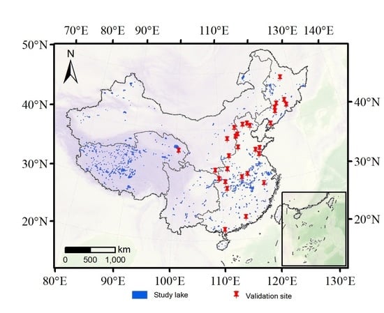
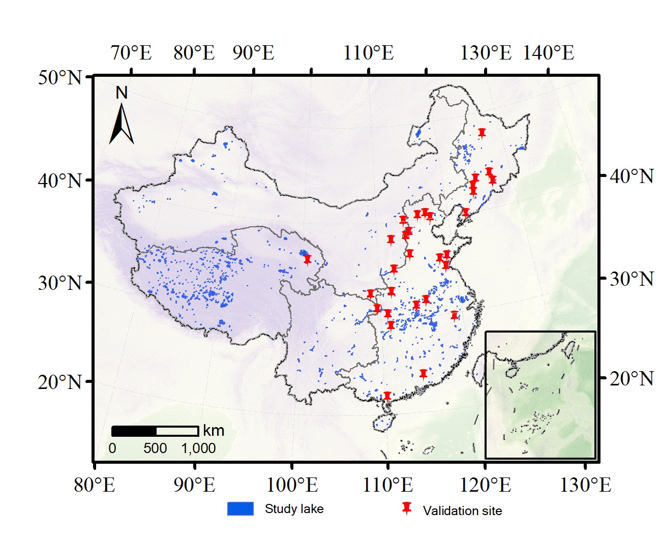
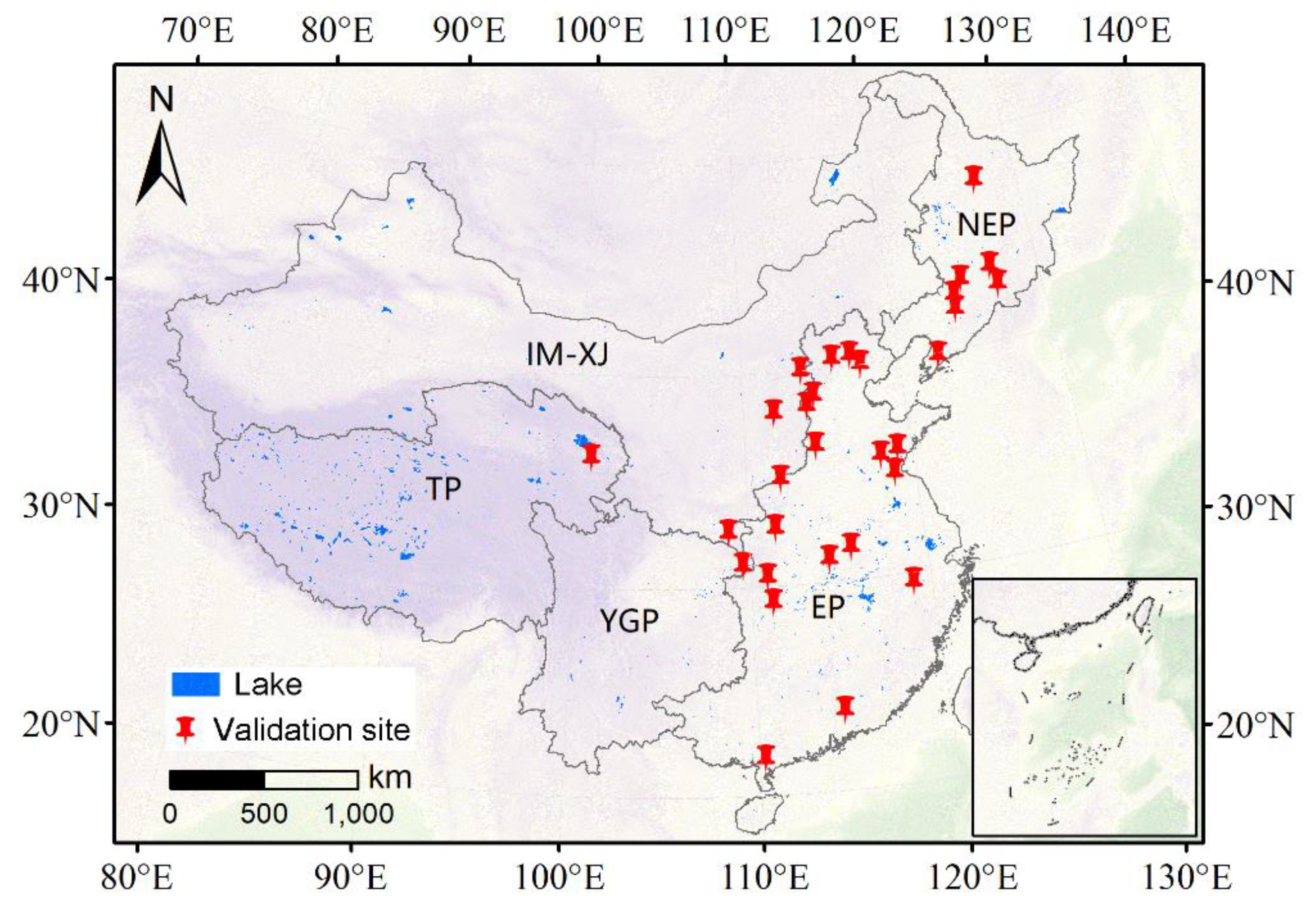
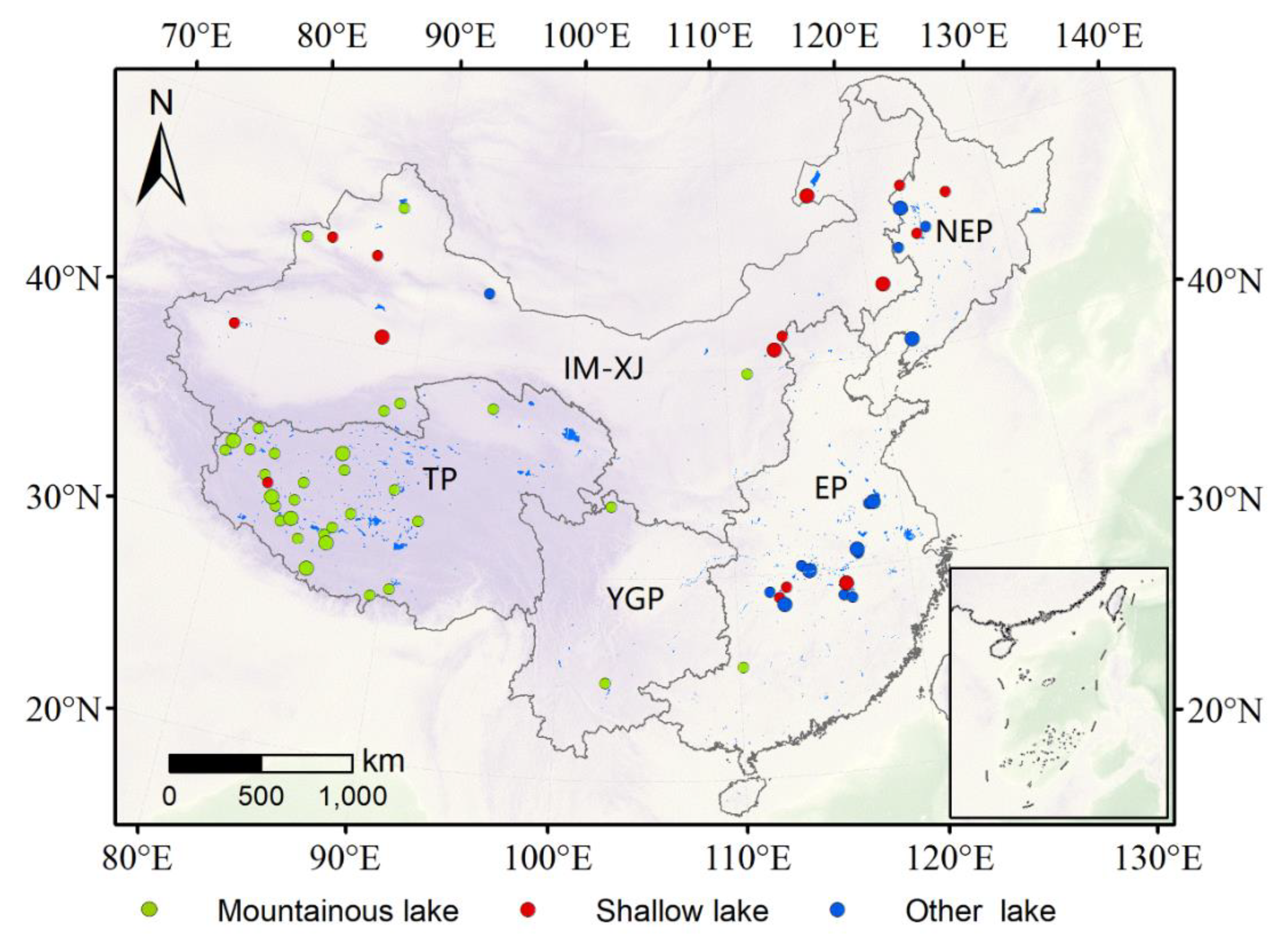
We studied all lakes and reservoirs greater than 10 km² in China (Figure 1), which include most lake types worldwide. There are numerous high-altitude lakes in the Tibetan plateau (TP), floodplain lakes in the Eastern Plain (EP), high-latitude lakes in the Northeastern Plain (NEP), and shallow lakes in the Inner Mongolia–Xinjiang region (IM–XJ). The lake boundaries were delineated by HydroLAKES (https://www.hydrosheds.org/page/hydrolakes), which is a database providing shoreline polygons for global lakes greater than 0.1 km² [23]. Furthermore, we visually modified the boundaries in some places where surface water has varied greatly, with the aid of Google Earth.

2.2. ICESat-2

We utilized the latest ATLAS/ICESat-2 L3A (ATL13) product, which provides water surface height for inland water bodies. Up to 02 December 2019, data from 13 October 2018 to 2 May 2019 are available from the National Snow and Ice Data Center (NSIDC; https://nsidc.org/data/atl13) [25]. The ATL13 dataset provides along-track heights for lakes, rivers, and wetlands with reference to the Earth Gravitational Model 2008 (EGM2008). Along with the height product, quality control fields are also provided. We adopted the higher version of the ICESat-2 data if several versions were provided.

2.3. SARAL

We also collected altimetry data of the SARAL, which is the first Ka-band altimetry mission conducted by the Centre National d’Etudes Spatiales (CNES) and Indian Space Research Organization (ISRO). The SARAL has some improvements compared with traditional radar altimeters, in terms of footprint size, vertical range sampling interval, and along-track sampling rate, and it has demonstrated some advantages in lake monitoring [26,27,28,29].

The Sensor Geophysical Data Record (SGDR) of the SARAL from February 2013 to October 2019 (0–35 and 100–133 cycles) were downloaded from the CNES Archiving, Validation, and Interpretation of Satellite Oceanographic (AVISO+) team (ftp://avisoftp.cnes.fr/AVISO/). During the study period, SARAL operated in a repetitive orbit before 04 July 2016. After that, it started a drifting phase (DP) and its orbit decayed naturally.

2.4. ICESat

As the precursor of the ICESat-2, the ICESat was the first space-borne laser altimetry mission, and it operated from 2003 to 2009. We collected ICESat products over inland waters from the ICESat derived inland water surface spot heights (IWSH) database (https://0-data-bris-ac-uk.brum.beds.ac.uk/data/dataset) developed by the University of Bristol [30,31]. It is a freely accessible water-level database for water bodies wider than 3 arcsec (~93 m).

2.5. Gauge Data

Since December 2018, we collected the gauge water level of 30 reservoirs every day from China Hydrology (http://xxfb.mwr.cn/ssIndex.html) which publishes near real-time water level data for most Chinese reservoirs and rivers. To guarantee the quality of the collected data, we carefully checked the water-level time series of each reservoir. The gauge data were used to assess the altimetric precision of the ICESat-2. As a comparison, we also validated the SARAL-DP data with the same gauge data. However, the vertical datum is unknown and inconsistent because the sites are maintained by different agencies.

3. Method

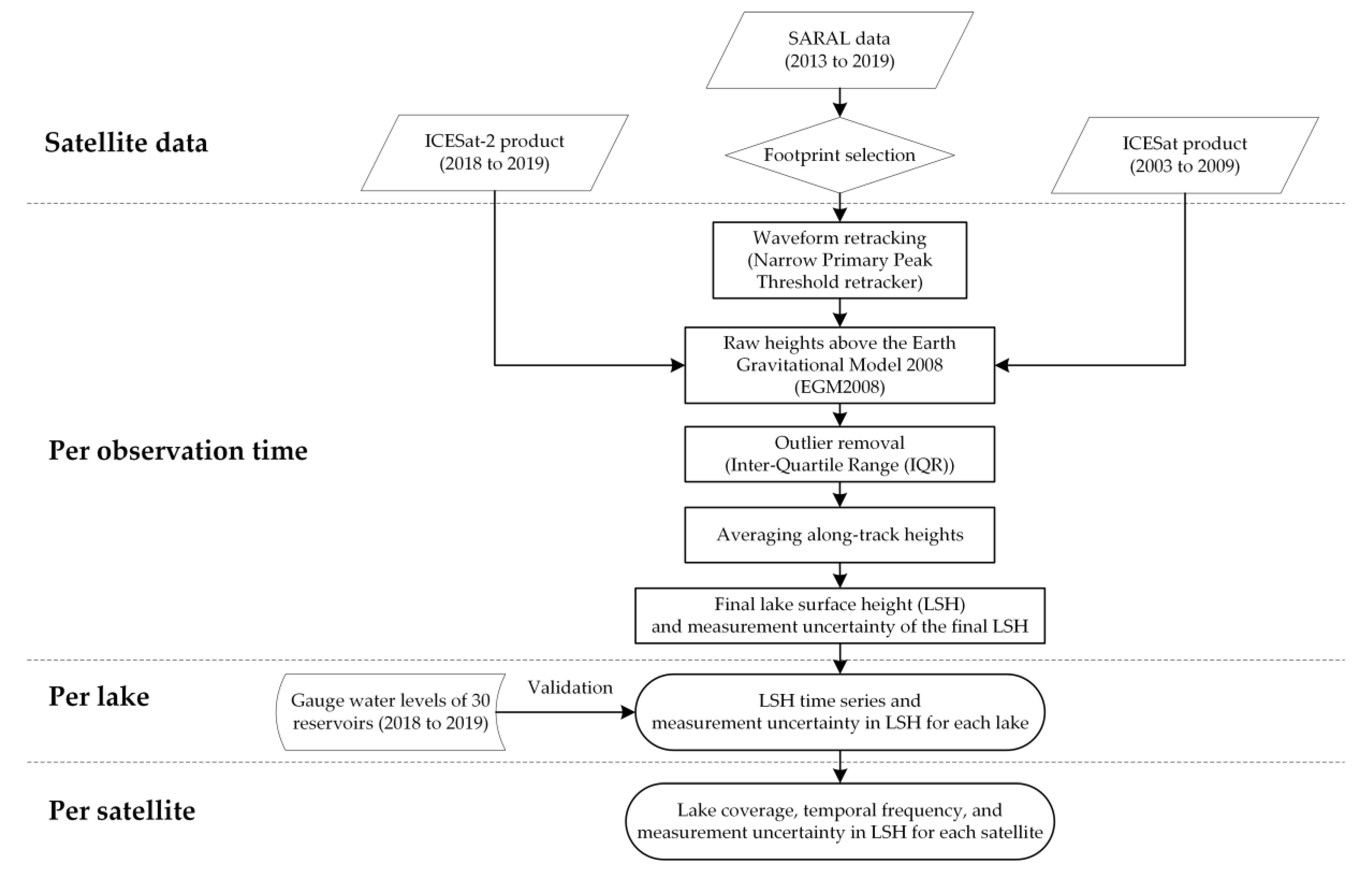
A satellite altimeter works by emitting and receiving pulse signals, and the satellite–ground distance can be estimated by recording the time lapse. We derived the altimetric LSH time series from the ICESat-2, SARAL, and the ICESat data. The ICESat-2 and ICESat products provide LSH results. SARAL data provide original ranges and we performed additional waveform retracking (described in Section 3.2) to derive precise LSHs. The workflow of LSH extraction is shown in Figure 2.

3.1. Extracting Water-Level Time Series from ICESat-2

There are three main steps to process the ICESat-2 ATL13 data. First, we utilized footprints within the lake boundary. Second, we derived the final LSH after dropping outliers and averaging along-track heights for each observation time. Finally, we constructed the LSH time series.

3.1.1. Lake Surface Height Extraction

When the ICESat-2 flies over a lake, numerous radar echoes return from the lake surface, owing to its dense along-track sampling rate and the configuration of six beams. To derive a reliable LSH, we averaged the along-track LSHs after outlier removal. To detect outliers, an inter-quartile range (IQR) method was applied, and mild outliers were detected by the 1.5 times of the difference between the third and first quartiles (1, 2).

$$\mathrm{IQR}=q_{0.75}-q_{0.25}$$

(1)

$${\mathrm{LSH}}_{outlier}>q_{0.75}+1.5\ast \mathrm{IQR} or {\mathrm{LSH}}_{outlier}<q_{0.25} - 1.5\ast \mathrm{IQR}$$

(2)

where $q_{0.25}$ and $q_{0.75}$ are the first and third quartiles of measured LSHs, ${\mathrm{LSH}}_{outlier}$ are the detected outliers which are beyond the fence [ $q_{0.25}$ − 1.5 $\mathrm{IQR}$, $q_{0.75}$ + 1.5 $\mathrm{IQR}]$.

3.1.2. Measurement Uncertainty in Water Surface Height Extraction

For each observation time, there are multiple observations ($x$) along-track. To describe the uncertainty of the final LSH per observation time, the standard deviation (SD) of observations (after outlier removal) is used as an evaluation index.

Each lake was observed multiple times. To represent the uncertainty of the lake, the median of SDs (MSD) of all observation times was taken as an evaluation index.

Each satellite observed a great number of lakes. To indicate the measurement uncertainty in LSH of the satellite, the median of MSDs (MMSD) of all lakes was taken as an evaluation index.

For MSD and MMSD, the median was used to indicate the magnitude of SD and MSD, because it is more robust to outliers and the frequency distribution of SD and MSD are positively skewed.

$$S{D}_j=\sqrt{\frac{{{\displaystyle \sum }}_{i=1}^m{\left(x_i-\overline{x}\right)}^2}{m}}$$

(3)

$$MS{D}_k=\mathrm{median}\left(S{D}_1,S{D}_2,\dots S{D}_n\right)$$

(4)

$$MMSD=\mathrm{median}\left(MS{D}_1,MS{D}_2,\cdots ,MS{D}_l\right)$$

(5)

where $i$, $j$, $k$ are the $i$-th observations at the $j$-th time for the $k$-th lake, and $m$, $n$ and $l$ are the number of along-track observations, observation times and covered lakes, respectively.

3.2. Extracting Water-Level Time Series from the SARAL and ICESat

Different from laser altimeters, SARAL has a relatively great footprint size (1.40 km) and some lakes face a waveform pollution problem. Thus, we processed the original waveform data of SARAL to alleviate waveform pollution. To exclude observations of poor quality, we developed a footprint selection procedure that preserved valid SARAL footprints with an automatic gain control (AGC) greater than 30 dB or corrected backscatter coefficient Sig0 greater than 10 dB, by analyzing substantial footprints on different types of ground. The basic principle of deriving an LSH is by subtracting the satellite-ground range ($R_0$) from the satellite altitude ($H_{\mathrm{sat}}$). To get a precise epoch when the radar altimeter illuminates the lake, we applied a Narrow Primary Peak Threshold retracker (NPPT) [32] to get a range correction ($\Delta R$). NPPT takes the subwaveform of maximum energy as the water reflection considering the strong reflection characteristics of water, and it has been widely applied to investigate Chinese lakes and reservoirs [33,34].

Considering the in-path time delay, we also applied troposphere (wet and dry) correction ($R_{td} \mathrm{and} R_{tw}$) and ionosphere correction ($R_I$). Finally, geophysical correction was applied, including pole tide and solid earth tide correction ($C_{\mathrm{pt}} \mathrm{and}{C}_{\mathrm{set}}$) and vertical datum correction ($C_{\mathrm{geoid}}$; from ellipsoid height to EGM2008 height).

$$\mathrm{LSH}=H_{\mathrm{sat}}-\left(R_0+\Delta R+R_{td}+R_{tw}+R_I\right)-C_{\mathrm{pt}}-C_{\mathrm{set}}-C_{\mathrm{geoid}}$$

(6)

As with ICESat-2, we applied the same outlier removal method for SARAL and ICESat per cycle and the average height is taken as the final LSH. To assess the uncertainty of the LSH time series of each lake, the MSD was calculated, and the MMSD of all lakes was calculated to indicate the measurement uncertainty of each satellite.

3.3. Evaluating the Altimetric Precision of ICESat-2 and SARAL

Comparing altimetric water levels with gauge water levels from the same day, we evaluated the altimetric precision of ICESat-2 and SARAL over 30 reservoirs. Three evaluation metrics were used: (1) mean absolute error (MAE); (2) SD; and (3) Pearson correlation coefficient (CC).

MAE and SD describe the absolute and relative altimetric error of the derived LSH time series. To be specific, MAE and SD are the mean and standard deviation of the difference between the altimetric heights and gauge water levels. CC describes the correlation relationship between the two data sources. The formulations of the three metrics are as below:

$$\mathrm{MAE}=\frac{{{\displaystyle \sum }}_{p=1}^N\left(h_p-H_p\right)}{N}$$

(7)

$$\mathrm{SD}=\sqrt{\frac{{{\displaystyle \sum }}_{p=1}^N{\left(\left(h_p-H_p\right)-MAE\right)}^2}{N}}$$

(8)

$$\mathrm{CC}=\frac{{{\displaystyle \sum }}_{p=1}^N\left(h_p-\overline{h}\right)\left(H_p-\overline{H}\right)}{\sqrt{{{\displaystyle \sum }}_{p=1}^N{\left(h_p-\overline{h}\right)}^2}\sqrt{{{\displaystyle \sum }}_{p=1}^N{\left(H_p-\overline{H}\right)}^2}}$$

(9)

where $h$ is altimetric water level, H is gauge water level, p is the p-th validation data, N is the number of validation data, $\overline{h}$ is the average of altimetric water levels, and $\overline{H}$ is the average of gauge water levels.

4. Results and Discussion

From October 2018 to May 2019, the ICESat-2 has covered about three-fourths of lakes (636 out of 862) of HydroLAKES. Note that ‘lake’ is a general term in places where the distinction between lake and reservoir is not critical. Due to the short time span (about seven months), 61% of all lakes have only one or two observations, and some large lakes with narrow shapes have more observations. Lake Hulun has the maximum observation number (15 times).

4.1. Altimetric Precision of the ICESat-2 Data

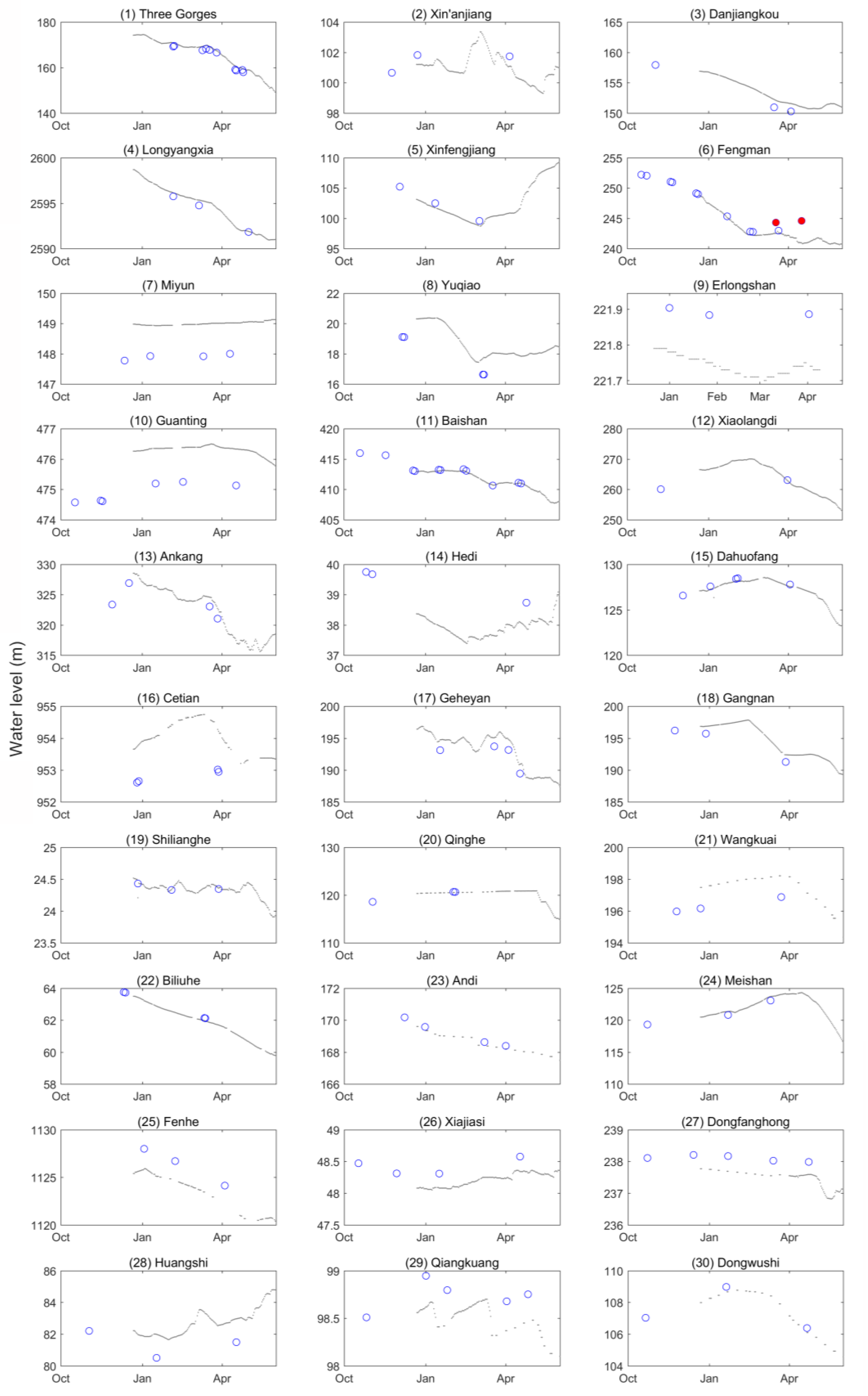
The performance of the ICESat-2 has been validated over 30 reservoirs (Figure 3). Altimetric LSHs are in good consistency with gauge records, even though the systematic bias may not be uniform because the vertical datums are different. The specific validation results and evaluation metrics are listed in

Table A1. Validation results of ICESat-2 and SARAL over 30 reservoirs.

ID	Name	Latitude (°)	Longitude (°)	Area (km2)	ICESat-2					SARAL
					MSD (m)	Num	MAE (m)	SD (m)	CC	No Footprint Selection		After Footprint Selection (This Study)
										Num	MAE (m)	MSD (m)	Num	MAE (m)	SD (m)	CC
1	Three Gorges	30.35	108.88	852	0.01	10	−1.35	0.40	1.00 **	34	365.96	5.11	1	113.32	/	/
2	Xin‘anjiang	29.60	118.92	424	0.03	2	0.64	0.03	1.00	10	−19.38	0.26	7	0.05	2.18	0.78 *
3	Danjiangkou	32.68	111.35	286	0.02	2	−1.31	0.01	1.00	8	43.83	0.34	5	-2.09	1.64	0.95 **
4	Longyangxia	36.03	100.71	285	0.02	3	−0.35	0.27	1.00 *	7	0.39	0.09	7	0.36	0.24	0.99 **
5	Xinfengjiang	23.90	114.53	264	0.02	2	0.77	0.00	1.00	7	74.36	0.27	4	0.63	0.21	0.99 **
6	Fengman	43.46	126.96	194	0.02	6	1.16	1.32	0.43	7	33.40	0.15	4	12.62	20.87	−0.83
7	Miyun	40.51	116.93	122	0.01	3	−1.04	0.03	0.73	4	22.29	0.37	2	−2.02	2.24	−1.00
8	Yuqiao	40.04	117.59	119	0.03	2	−1.10	0.05	−1.00	4	−23.37	0.22	2	1.29	1.83	−1.00
9	Erlongshan	43.20	124.86	98	0.03	3	0.13	0.01	0.94	2	0.66	0.17	2	0.66	0.25	1.00
10	Guanting	40.35	115.73	90	0.02	3	−1.16	0.03	0.99	3	31.15	0.20	2	−0.48	0.25	1.00
11	Baishan	42.54	127.35	85	0.02	7	0.11	0.08	1.00 *	5	44.41	0.16	4	0.53	0.43	0.89
12	Xiaolangdi	34.99	112.07	62	0.02	1	0.13	/	/	4	106.33	/	/	/	/	/
13	Ankang	32.54	108.68	57	0.02	2	−1.61	0.12	1.00	1	168.07	/	/	/	/	/
14	Hedi	21.80	110.33	52	0.02	1	0.84	/	/	3	1.79	0.19	3	1.79	0.28	1.00 *°
15	Dahuofang	41.88	124.21	51	0.01	4	0.27	0.02	1.00 **	5	16.62	0.25	4	9.90	20.90	0.39
16	Cetian	39.92	113.64	47	0.01	4	−1.20	0.08	1.00 **	3	76.10	/	/	/	/	/
17	Geheyan	30.42	110.89	41	0.01	4	−1.53	0.15	1.00 **	2	173.65	/	/	/	/	/
18	Gangnan	38.34	113.93	39	0.02	2	−1.14	0.03	1.00	5	33.14	0.39	2	−0.70	0.08	1.00
19	Shilianghe	34.78	118.81	39	0.01	3	0.07	0.12	−0.97	2	0.58	0.17	1	0.80	/	/
20	Qinghe	42.54	124.29	37	0.02	2	0.14	0.02	/	3	24.92	0.31	2	19.71	26.97	−1.00
21	Wangkuai	38.77	114.42	34	0.01	2	−1.33	0.01	1.00	/	/	/	/	/	/	/
22	Biliuhe	39.87	122.49	32	0.02	2	0.17	0.01	1.00	/	/	/	/	/	/	/
23	Andi	35.69	118.08	26	0.02	2	0.21	0.03	1.00	/	/	/	/	/	/	/
24	Meishan	31.60	115.82	25	0.02	2	−0.58	0.06	1.00	1	121.78	/	/	/	/	/
25	Fenhe	38.09	111.88	21	0.01	1	2.12	/	/	1	−134.21	/	/	/	/	/
26	Xiajiasi	31.09	114.48	18	0.01	2	0.23	0.01	1.00	1	4.95	0.16	1	4.95	/	/
27	Dongfanghong	47.66	127.16	17	0.01	2	0.44	0.06	1.00	/	/	/	/	/	/	/
28	Huangshi	29.23	111.14	16	0.02	2	−1.48	0.01	1.00	1	−0.58	0.07	1	−0.58	/	/
29	Qiangkuang	35.86	119.15	14	0.02	2	0.32	0.01	1.00	1	1.20	0.13	1	1.20	/	/
30	Dongwushi	36.41	114.28	12	0.01	2	0.30	0.02	1.00	1	94.52	/	/	/	/	/

The number of validation data (‘Num’), measurement uncertainty (‘MSD’), absolute altimetric error (‘MAE’), relative altimetric error (‘SD’), and Pearson correlation coefficient (‘CC’) are shown. Note that symbol ‘**’ and ‘*’ in the top right corner of ‘CC’ indicates the significance of ‘CC’ at the confidence level of 0.01 and 0.05, and abnormal MAEs (>5 m) and SDs (>5 m) are in bold italics.

. Generally, no great absolute error was found (|MAE| < 5 m) and the relative error was generally low (SD < 0.50 m), except for Fengman Reservoir (SD = 1.32 m). To be specific, 21 reservoirs had a small SD, ranging from 0.00 m to 0.10 m. Five reservoirs had a moderate SD, ranging from 0.10–0.50 m. The great relative error of Fengman Reservoir was mainly caused by two abnormal observations (Figure 3(6)) when the reservoir began to thaw and when the stream bed was exposed as the water level dropped. In general, the mean relative error was 0.06 m for ICESat-2 if Fengman Reservoir was excluded.

As a comparison, we also validated the SARAL results with the same gauge data. From Table A1, we found that the ICESat-2 data has a superior measurement capability in LSH to the SARAL from the following aspects.

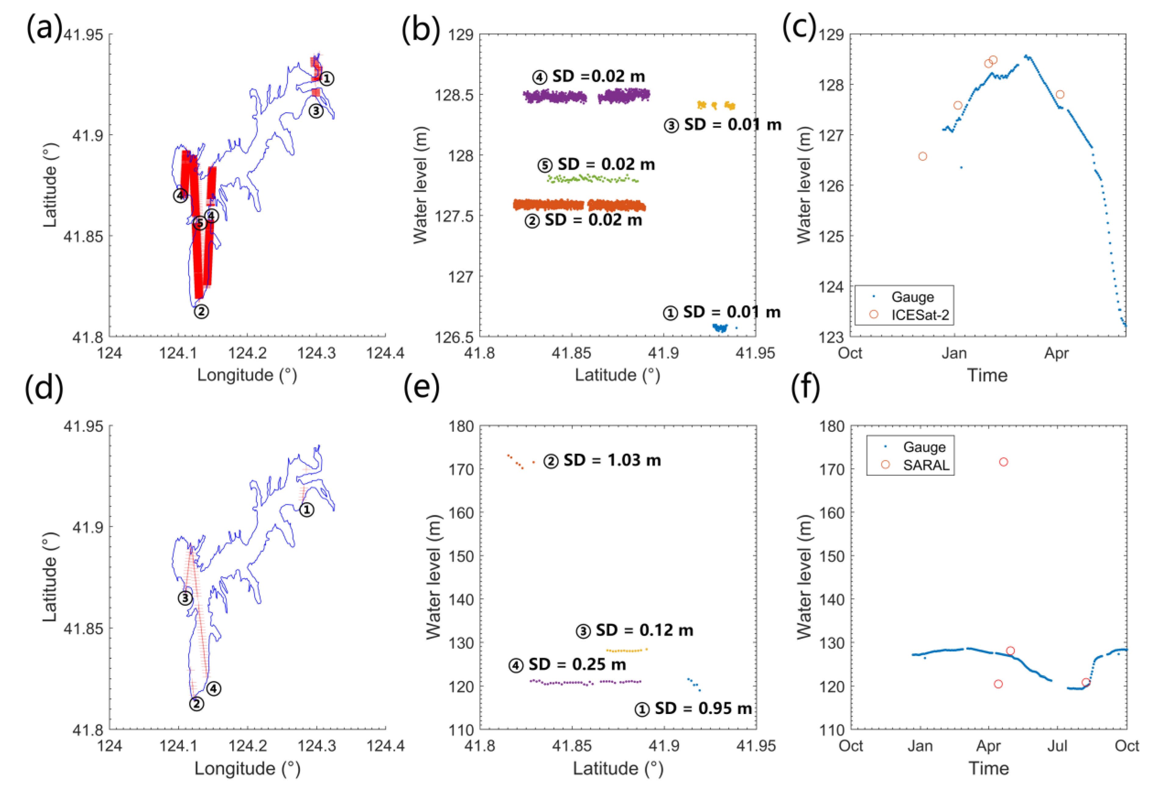
First, the ICESat-2 is less likely to be locked in surrounding mountains. For the SARAL, the length of range window is about 30 m, and the observed height is invalid and much higher than LSH (>30 m) if the range window has not been well adjusted to water surface. During our short validation time span, a reservoir with a large MAE (>5 m) indicates that it has invalid observations. Were no footprint selection was applied, only seven reservoirs would have reliable results (MAE<5 m). In this study, 15 reservoirs had reliable results following our footprint selection procedure, while all 30 reservoirs had reliable results for the ICESat-2. Although the SARAL has adopted an open-loop tracking mode when it flies over a narrow reservoir surrounded by mountains, the onboard tracking window may be locked at mountains and the weak water reflection has not been recorded. The ICESat-2 adopts three strong–weak beam pairs, which enables it to capture the weak water reflection. Take the Dahuofang Reservoir as an example, when the SARAL crossed the reservoir shore the second time (Figure 4d), the tracking window missed the water reflection, and the estimated water level was about 50 m higher than normal (Figure 4f). In contrast, though the ICESat-2 crossed the reservoir shore the first and third time (Figure 4a), it successfully captured the water reflection signal and no invalid heights are recorded in Figure 4c.

Second, the ICESat-2 captured a more precise LSH than the SARAL (0.06 m vs. 0.25 m in relative altimetric error), owing to its small footprint, dense sampling, and multi-beams characteristics. The SARAL results had a poor consistency with gauge records, and the relative error ranged from 0.08–2.24 m. To be specific, 11 reservoirs had normal SDs (<5 m). Among them, one reservoir had a small SD (<0.1 m), six reservoirs had moderate SDs (0.1 m–0.5 m), and four reservoirs had great SDs (>0.5 m). In general, the relative altimetric error was 0.25 m for the SARAL (four great SDs were excluded). Take the Dahuofang Reservoir as an example, when the satellite crossed the lake shore, the along-track LSHs varied greatly for the SARAL, while they were highly uniform for the ICESat-2 (Figure 4b,e).

4.2. Comparison with the SARAL and ICESat in Lake Coverage and Temporal Frequency

Different from optical images, space-borne altimeters only record data in the nadir direction and many regions are not monitored. To evaluate their capability in monitoring lake dynamics and lake seasonality at large scale, lake coverage and temporal frequency are two important factors. Out of the 862 lakes and reservoirs (>10 km²) studied here, the number of observed ones was used to indicate the lake coverage, and the median of annual observation frequency of covered lakes was used to indicate the temporal frequency.

Compared with SARAL and ICESat, ICESat-2 had a greatly improved spatial-temporal coverage in lake monitoring.

Table 2. Statistics on lake observations derived from the ICESat-2, ICESat, and SARAL data.

Satellite	Time Period	Number of Observed Lakes	Annual Observation Frequency	MMSD (m)
ICESat-2	2018.10–2019.05	636	3.43	0.02
SARAL (Repeat Phase, Drifting Phase)	2013.03–2019.10 (before 2016.07, after 2016.07)	814 (479, 802)	1.35 (2.63, 1.85)	0.17 (0.13, 0.15)
ICESat	2003.02–2009.10	311	1.48	0.07

The maximum number of observed lakes, maximum annual observation time and minimum measurement uncertainty (‘MMSD’) among the three satellites are in bold.

shows the statistics of lake coverage and temporal frequency of the three satellites. Compared with the SARAL, the ICESat-2 had a greatly densified temporal frequency (3.43 vs. 1.35), though the lake coverage decreased by a fifth (636 vs. 814). When the SARAL operated in the repeat orbit, the ICESat-2 had a wider lake coverage (636 vs. 479) and a denser temporal frequency (3.43 vs. 2.63). When the SARAL operated in a decaying orbit, the SARAL-DP data covered more lakes and the temporal frequency decreased as a compromise. Compared with the SARAL-DP data, the ICESat-2 data had a sparser lake coverage (636 vs. 802) and a denser temporal frequency (3.43 vs. 1.85). Compared with the ICESat, the ICESat-2 has a greatly densified lake coverage (636 vs. 311) and temporal frequency (3.43 vs. 1.48). In addition, the ICESat-2 tends to cover more lakes in the future, owing to an off-nadir pointing strategy over land areas.

4.3. Comparison with the SARAL and ICESat in Measurement Uncertainty

The final LSH of each observation time was derived by averaging the along-track heights after excluding outliers, which was of great uncertainty if the LSH profile was non-horizontal. MSD is a summary of measurement uncertainty for each lake, and MMSD is a summary of MSD for each satellite.

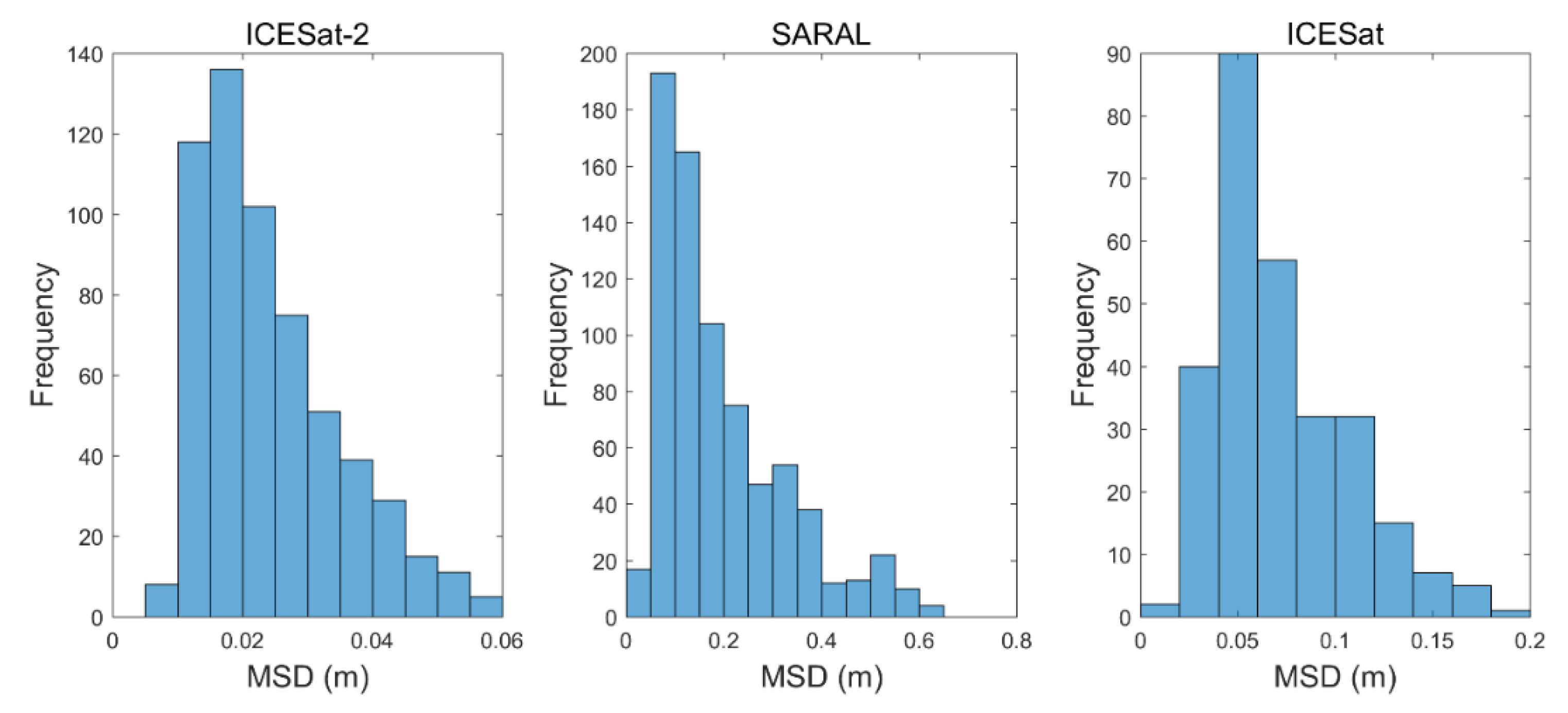
Compared with the SARAL and ICESat, the ICESat-2 had a considerably decreased measurement uncertainty (Figure 5) with an MMSD of 0.02 m (Table 2), compared to 0.17 m and 0.07 m for the SARAL and ICESat, respectively. It should be noted that the measurement capability of the SARAL was well maintained during the two phases [35], and the MMSD was comparable during the two phases (0.13 m vs. 0.15 m).

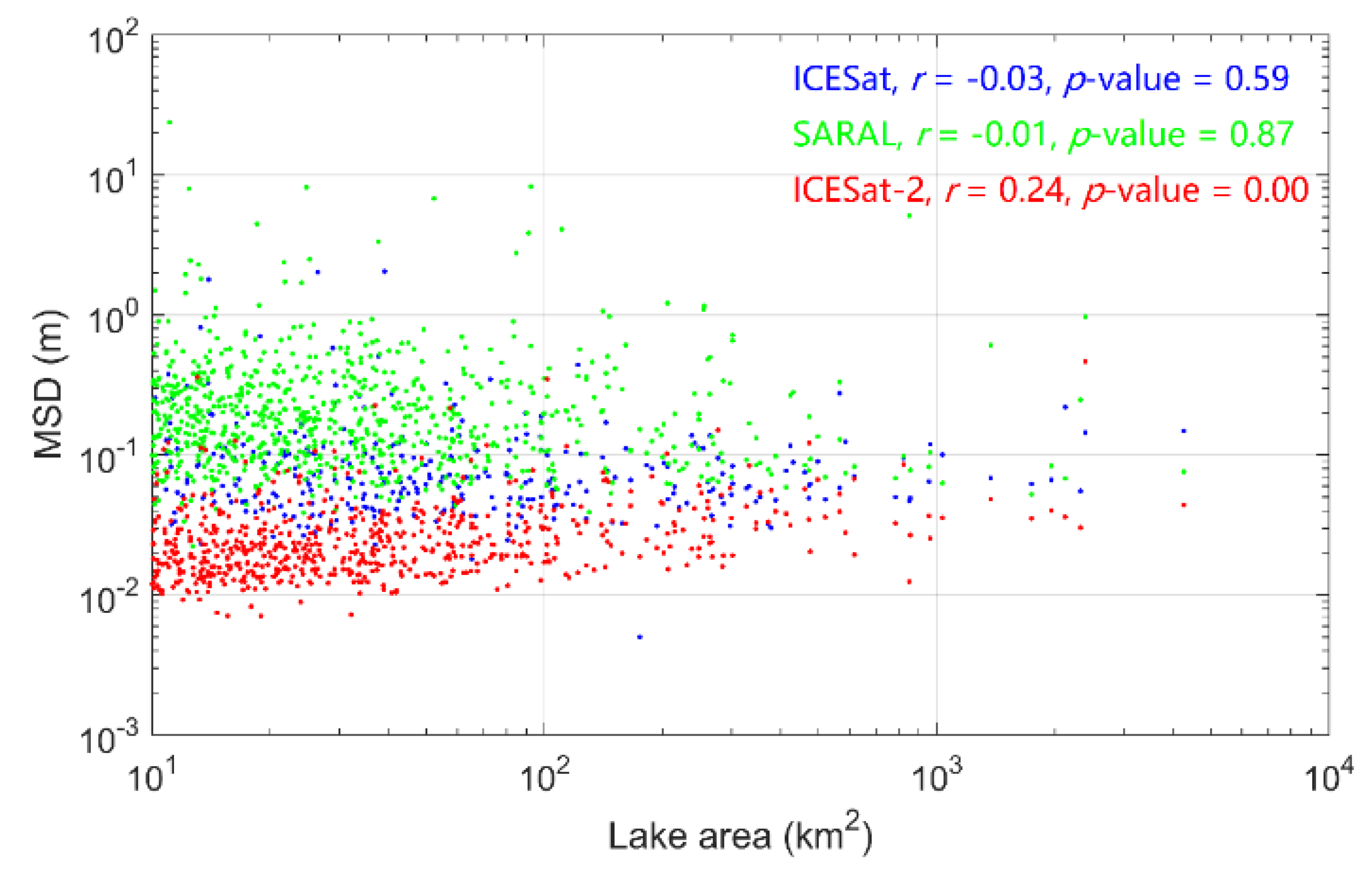
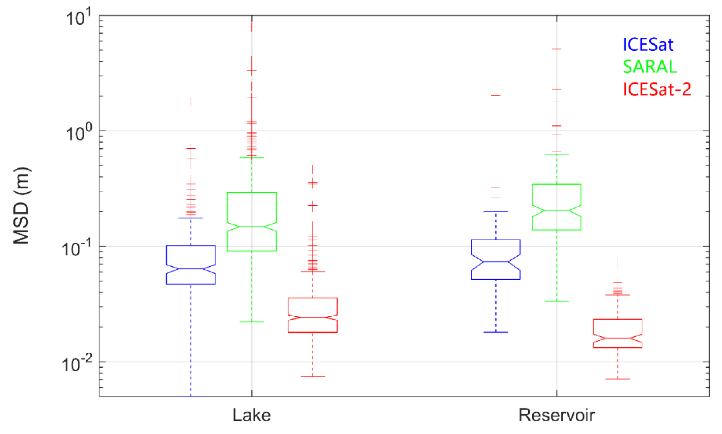
From the relationship between lake area and MSD (Figure 6), we found that the ICESat-2 had a significant positive correlation between MSD and lake area (r = 0.24, p-value = 0.00), suggesting that large lakes tend to have a great measurement uncertainty, while the relationship was not found for the ICESat and SARAL. It confirms that waveform pollution is no longer the main error source for the altimetric LSHs derived from the ICESat-2 data. Non-horizontal lake surface may be the main error source because large lakes usually have long cross sections. However, for the ICESat and SARAL, both waveform pollution and non-horizontal lake surface lead to the discrepancy of along-track heights. Thus, the correlation relationship was weak. In addition, the ICESat-2 had superior performance over reservoirs than lakes, which is in contrast to the ICESat or SARAL (Figure 7). Generally, reservoirs are located in rugged terrains with narrow shapes and long tails. The short cross section length may contribute to the small MSD.

4.4. Causes of Non-Horizontal LSH Profile for the ICESat-2

Different from point-based gauge stations, satellite altimetry measures multiple LSHs along-track. For the ICESat-2, the LSH of each footprint should be precise, considering its advanced altimetric capability. However, the final LSH may be of great uncertain if the LSH profile is not horizontal. We derived the MSDs of 636 lakes and found that 90% of all lakes had a quasi-horizontal LSH profile, with a small MSD varying from 0.01–0.05 m, while 63 lakes had a non-horizontal LSH profile (Figure 8). To be specific, 46 lakes had a moderate MSD (from 0.05–0.10 m), and 17 lakes had a great MSD (>0.10 m). By checking into the 63 lakes, we found that there were mainly three types of lakes. First, mountainous lakes in plateaus or valleys, such as the lakes in the Tibetan plateau (TP). Second, shallow lakes in arid regions or plains, such as the lakes in the Inner Mongolia–Xinjiang (IM–XJ) lake zone. Third, other lakes in plains or coastal areas, such as the lakes in the Eastern Plain (EP) and Northeastern Plain (NEP) zones. By checking into the LSH profiles, we think that the measurement uncertainty is closely related to geopotential undulation, lake mask, and lake flatness.

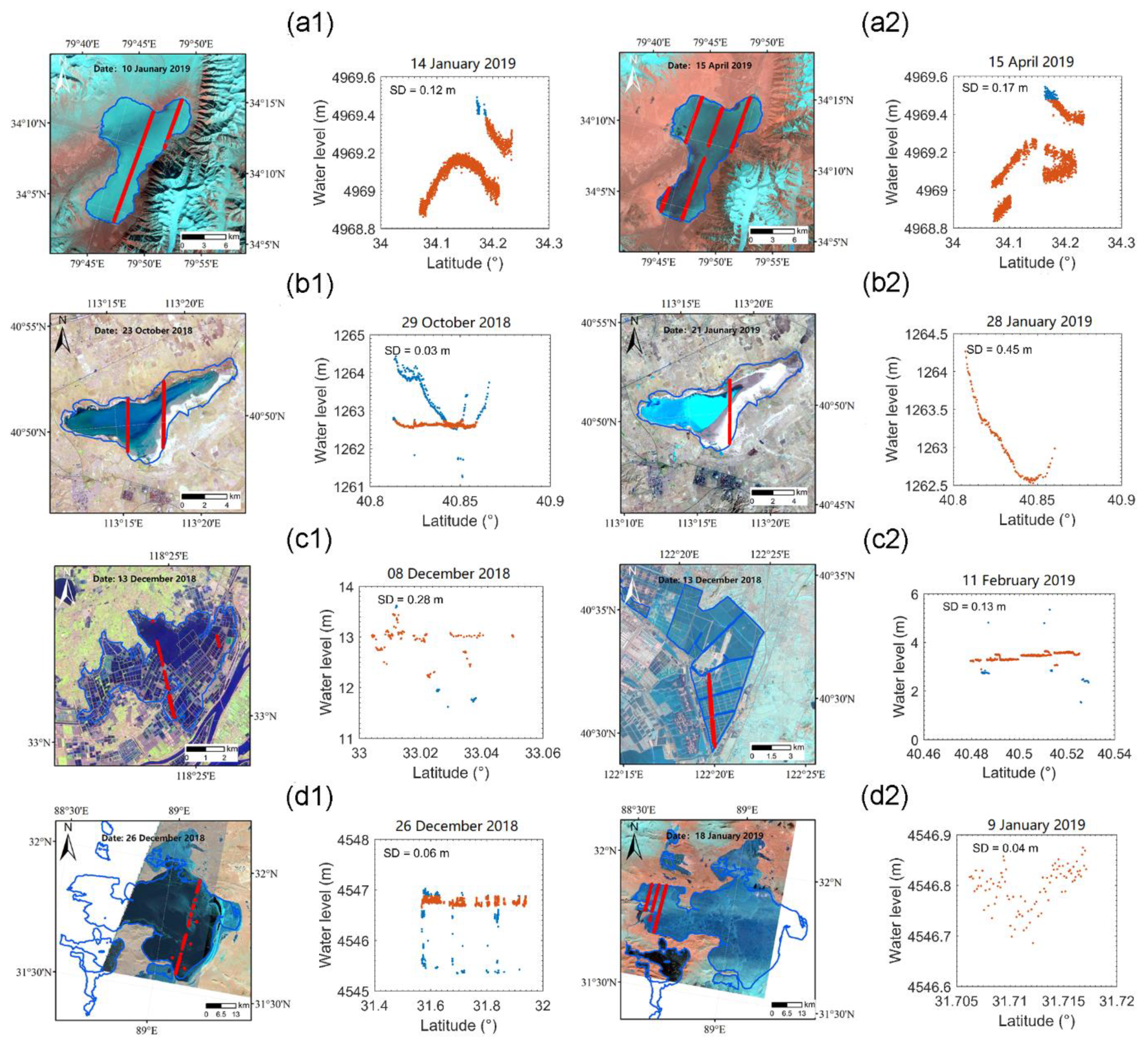
Geopotential undulation is an important cause of non-horizontal LSH profiles, especially for mountainous lakes, such as the lakes in the TP. Under the force of gravity, the lake surface follows the geopotential surface if the lake is calm. Unlike the geoidal surface where the gravitational potential energy equals zero, lake surface describes the shape of another geopotential of certain potential energy, and the two surfaces are neither parallel nor crossed. We used the geoid model EGM2008 as the elevation reference, and the lake surface might not be parallel to it, thus the observed LSH profile was irregular. In the TP, geopotential surface fluctuates greatly due to the uneven distribution of earth mass, and the discrepancy between geoid models may vary by up to several meters [36]. The observed along-track and inter-track discrepancy can reach several decimeters. For example, an alpine lake named Ze Co (Figure 9a1,a2) has a maximum elevation difference of ~0.60 m. At the two observation times, the LSH profile was similar for the longest cross section, and it suggests that the measurement uncertainty is a systematic error and it is hard to eliminate.

Lake mask is another important cause of non-horizontal LSH profile, especially for shallow lakes. Shallow lakes tend to have a large SD when the lake bed is exposed. For example, Lake Huangqihai, a shallow lake in Inner Mongolia, has a dramatic water area change in different seasons (Figure 9b1,b2), and the LSH profile may describe the lake bed profile when the lake dries up. It indicates that an advanced outlier removal method [37] or a dynamic water mask [38] is needed for shallow lakes, rather than adopting all footprints in a fixed lake boundary.

Uneven lake surface may also cause a non-horizontal LSH profile, especially for partitioned lakes or frozen lakes. Partitioned lakes may be separated into multiple fish ponds, and the observed profiles depict the elevation difference between ponds. In Figure 9c1,c2, the two lakes along the Yangtze River and Bohai Bay are partitioned, and the LSH profiles are irregular. It indicates that the LSH profile may be a good indicator of lake connectivity. In addition, high-altitude or high-latitude lakes tend to freeze in winter, and an irregular profile may be observed when the lake is not completely ice-covered. For example, when Selin Co was not completely frozen (Figure 9d1), the lake surface was irregular, while it was flat when the lake was completely frozen (Figure 9d2). It suggests that the ICESat-2 data may be valuable for the study of lake ice phenology [39,40].

5. Conclusions

In this study, we evaluated the altimetric precision of ICESat-2 ATL13 data using gauge data collected from 30 reservoirs. To explore the ICESat-2′s capability in large-scale lake monitoring, we applied it to investigate all lakes and reservoirs (>10 km²) in China, in terms of lake coverage, temporal frequency, and measurement uncertainty. To demonstrate its improvement with previous missions, we also applied the ICESat and SARAL to investigate all Chinese lakes and reservoirs.

Based on the evaluation result, we found that the ICESat-2 demonstrated an advanced altimetric capability in LSH extraction, and the relative error was about 0.06 m, while it was 0.25 m for the SARAL. The ICESat-2 also showed superior capability in large-scale lake monitoring. Compared with the ICESat, the lake coverage and the temporal frequency increased by 104% and 132%, and the measurement uncertainty decreased from 0.07 m to 0.02 m. Compared with the SARAL, the temporal frequency increased by 154%, and the measurement uncertainty decreased from 0.17 m to 0.02 m, though the lake coverage decreased by 22%. In addition, the precise LSH profiles delineated by the ICESat-2 data showed that most lakes (90% of 636 lakes) had a quasi-horizontal LSH profile and the measurement uncertainty was low (MSD < 0.05 m), while some mountainous and shallow lakes tended to have a large measurement uncertainty (MSD > 0.05 m).

This study provides an extensive assessment of ICESat-2 data. ICESat-2 has a bright prospect in monitoring lake dynamics and revealing lake seasonal patterns at large scale. This study further suggests that the routine method (take the median or mean) may be acceptable in determining the final LSH from multiple along-track heights. Dedicated methods are needed for some mountainous lakes or shallow lakes, to alleviate errors caused by geopotential undulation or inaccurate water mask.

References

- Robertson, D.M.; Ragotzkie, R.A. Changes in the thermal structure of moderate to large sized lakes in response to changes in air temperature. Aquat. Sci. 1990, 52, 360–380. [Google Scholar] [CrossRef]
- De Wit, M.; Stankiewicz, J. Changes in Surface Water Supply Across Africa with Predicted Climate Change. Science 2006, 311, 1917–1921. [Google Scholar] [CrossRef] [PubMed] [Green Version]
- Vorosmarty, C.J. Global Water Resources: Vulnerability from Climate Change and Population Growth. Science 2000, 289, 284–288. [Google Scholar] [CrossRef] [Green Version]
- Alsdorf, D.E.; Lettenmaier, D.P. Tracking Fresh Water from Space. Science 2003, 301, 1491–1494. [Google Scholar] [CrossRef] [PubMed] [Green Version]
- Crétaux, J.F.; Abarca-del-Río, R.; Bergé-Nguyen, M.; Arsen, A.; Drolon, V.; Clos, G.; Maisongrande, P. Lake Volume Monitoring from Space. Surv. Geophys. 2016, 37, 269–305. [Google Scholar] [CrossRef] [Green Version]
- Alsdorf, D.E.; Rodríguez, E.; Lettenmaier, D.P. Measuring surface water from space. Revi. Geophys. 2007, 45. [Google Scholar] [CrossRef]
- Van Den Hoek, J.; Getirana, A.; Jung, H.C.; Okeowo, M.A.; Lee, H. Monitoring Reservoir Drought Dynamics with Landsat and Radar/Lidar Altimetry Time Series in Persistently Cloudy Eastern Brazil. Remote Sens. 2019, 11, 827. [Google Scholar] [CrossRef] [Green Version]
- Yu, C. Chinas water crisis needs more than words. Nature 2011, 470, 307. [Google Scholar] [CrossRef]
- Vorosmarty, C.; Askew, A.; Grabs, W.; Barry, R.G.; Birkett, C.; Doll, P.; Goodison, B.; Hall, A.; Jenne, R.; Kitaev, L.; et al. Global water data: A newly endangered species. Eos Trans. Am. Geophys. Union 2001, 82, 54. [Google Scholar] [CrossRef]
- Birkett, C.M. The contribution of TOPEX/POSEIDON to the global monitoring of climatically sensitive lakes. J. Geophys. Res. 1995, 100, 25179. [Google Scholar] [CrossRef]
- Crétaux, J.-F.; Birkett, C. Lake studies from satellite radar altimetry. C R. Geosci. 2006, 338, 1098–1112. [Google Scholar] [CrossRef]
- Crétaux, J.F.; Jelinski, W.; Calmant, S.; Kouraev, A.; Vuglinski, V.; Bergé-Nguyen, M.; Gennero, M.C.; Nino, F.; Abarca Del Rio, R.; Cazenave, A.; et al. SOLS: A lake database to monitor in the Near Real Time water level and storage variations from remote sensing data. Adv. Space Res. 2011, 47, 149–1507. [Google Scholar] [CrossRef]
- Schwatke, C.; Dettmering, D.; Bosch, W.; Seitz, F. DAHITI—an innovative approach for estimating water level time series over inland waters using multi-mission satellite altimetry. Hydrol. Earth Syst. Sci. 2015, 19, 4345–4364. [Google Scholar] [CrossRef] [Green Version]
- Zhang, G.; Xie, H.; Kang, S.; Yi, D.; Ackley, S.F. Monitoring lake level changes on the Tibetan Plateau using ICESat altimetry data (2003–2009). Remote Sens. Environ. 2011, 115, 1733–1742. [Google Scholar] [CrossRef]
- Wang, X.; Gong, P.; Zhao, Y.; Xu, Y.; Cheng, X.; Niu, Z.; Luo, Z.; Huang, H.; Sun, F.; Li, X. Water-level changes in Chinas large lakes determined from ICESat/GLAS data. Remote Sens. Environ. 2013, 132, 131–144. [Google Scholar] [CrossRef]
- Markus, T.; Neumann, T.; Martino, A.; Abdalati, W.; Brunt, K.; Csatho, B.; Farrell, S.; Fricker, H.; Gardner, A.; Harding, D.; et al. The Ice, Cloud, and land Elevation Satellite-2 (ICESat-2): Science requirements, concept, and implementation. Remote Sens. Environ. 2017, 190, 260–273. [Google Scholar] [CrossRef]
- Zhang, G.; Chen, W.; Xie, H. Tibetan Plateaus Lake Level and Volume Changes From NASAs ICESat/ICESat-2 and Landsat Missions. Geophys. Res. Lett. 2019, 46, 13107–13118. [Google Scholar] [CrossRef]
- Yuan, C.; Gong, P.; Liu, C.; Ke, C. Water-volume variations of Lake Hulun estimated from serial Jason altimeters and Landsat TM/ETM+ images from 2002 to 2017. Int. J. Remote Sens. 2018, 40, 670–692. [Google Scholar] [CrossRef]
- Jiang, L.; Andersen, O.B.; Nielsen, K.; Zhang, G.; Bauer-Gottwein, P. Influence of local geoid variation on water surface elevation estimates derived from multi-mission altimetry for Lake Namco. Remote Sens. Environ. 2019, 221, 65–79. [Google Scholar] [CrossRef]
- Kleinherenbrink, M.; Lindenbergh, R.C.; Ditmar, P.G. Monitoring of lake level changes on the Tibetan Plateau and Tian Shan by retracking Cryosat SARIn waveforms. J. Hydrol. 2015, 521, 119–131. [Google Scholar] [CrossRef]
- Phan, V.H.; Lindenbergh, R.; Menenti, M. ICESat derived elevation changes of Tibetan lakes between 2003 and 2009. Int. J. Appl. Earth Observ. Geoinfor. 2012, 17, 12–22. [Google Scholar] [CrossRef]
- Kleinherenbrink, M.; Ditmar, P.G.; Lindenbergh, R.C. Retracking Cryosat data in the SARIn mode and robust lake level extraction. Remote Sens. Environ. 2014, 152, 38–50. [Google Scholar] [CrossRef]
- Messager, M.L.; Lehner, B.; Grill, G.; Nedeva, I.; Schmitt, O. Estimating the volume and age of water stored in global lakes using a geo-statistical approach. Nat. Commun. 2016, 7, 13603. [Google Scholar] [CrossRef] [PubMed]
- Ma, R.; Duan, H.; Hu, C.; Feng, X.; Li, A.; Ju, W.; Jiang, J.; Yang, G. A half-century of changes in China’s lakes: Global warming or human influence? Geophys. Res. Lett. 2010, 37. [Google Scholar] [CrossRef]
- Jasinski, M.F.; Stoll, J.D.; Hancock, D.; Robbins, J.; Nattala, J.; Pavelsky, T.M.; Morison, J.; Arp, C.D.; Jones, B.M. The ICESat-2 Science Team. ATLAS/ICESat-2 L3A Inland Water Surface Height, Version 1; NASA National Snow and Ice Data Center Distributed Active Archive Center: Boulder, CO, USA, 2019. [Google Scholar] [CrossRef]
- Bonnefond, P.; Verron, J.; Aublanc, J.; Babu, K.; Bergé-Nguyen, M.; Cancet, M.; Chaudhary, A.; Crétaux, J.-F.; Frappart, F.; Haines, B.; et al. The Benefits of the Ka-Band as Evidenced from the SARAL/AltiKa Altimetric Mission: Quality Assessment and Unique Characteristics of AltiKa Data. Remote Sens. 2018, 10, 83. [Google Scholar] [CrossRef] [Green Version]
- Verron, J.; Bonnefond, P.; Aouf, L.; Birol, F.; Bhowmick, S.; Calmant, S.; Conchy, T.; Crétaux, J.-F.; Dibarboure, G.; Dubey, A.; et al. The Benefits of the Ka-Band as Evidenced from the SARAL/AltiKa Altimetric Mission: Scientific Applications. Remote Sens. 2018, 10, 163. [Google Scholar] [CrossRef] [Green Version]
- Kao, H.-C.; Kuo, C.-Y.; Tseng, K.-H.; Shum, C.K.; Tseng, T.-P.; Jia, Y.-Y.; Yang, T.-Y.; Ali, T.A.; Yi, Y.; Hussain, D. Assessment of Cryosat-2 and SARAL/AltiKa altimetry for measuring inland water and coastal sea level variations: A case study on Tibetan Plateau lake and Taiwan Coast. Mar. Geod. 2019, 1–17. [Google Scholar] [CrossRef]
- Arsen, A.; Crétaux, J.-F.; Abarca del Rio, R. Use of SARAL/AltiKa over Mountainous Lakes, Intercomparison with Envisat Mission. Mar. Geod. 2015, 38, 534–548. [Google Scholar] [CrossRef]
- OLoughlin, F.E.; Neal, J.; Yamazaki, D.; Bates, P.D. ICESat-derived inland water surface spot heights. Water Resour. Res. 2016, 52, 3276–3284. [Google Scholar] [CrossRef] [Green Version]
- Loughlin, F.O.; Bates, P.D.; Neal, J.C.; Yamazaki, D. ICESat Derived Inland Water Surface Spot Heights (IWSH). 2015. Available online: https://0-doi-org.brum.beds.ac.uk/10.5523/bris.15hbqgewcrti51hmzp69bi4gky (accessed on 2 December 2019).
- Jain, M.; Andersen, O.B.; Dall, J.; Stenseng, L. Sea surface height determination in the Arctic using Cryosat-2 SAR data from primary peak empirical retrackers. Adv. Space Res. 2015, 55, 40–50. [Google Scholar] [CrossRef]
- Jiang, L.; Nielsen, K.; Andersen, O.B.; Bauer-Gottwein, P. Monitoring recent lake level variations on the Tibetan Plateau using CryoSat-2 SARIn mode data. J. Hydrol. 2017, 544, 109–124. [Google Scholar] [CrossRef] [Green Version]
- Jiang, L.; Nielsen, K.; Andersen, O.B.; Bauer-Gottwein, P. CryoSat-2 radar altimetry for monitoring freshwater resources of China. Remote Sens. Environ. 2017, 200, 125–139. [Google Scholar] [CrossRef] [Green Version]
- Dibarboure, G.; Lamy, A.; Pujol, M.-I.; Jettou, G. The Drifting Phase of SARAL: Securing Stable Ocean Mesoscale Sampling with an Unmaintained Decaying Altitude. Remote Sens. 2018, 10, 1051. [Google Scholar] [CrossRef] [Green Version]
- Sjöberg, L.E.; Bagherbandi, M. Quasigeoid-to-geoid determination by EGM08. Earth Sci. Inform. 2012, 5, 87–91. [Google Scholar] [CrossRef]
- Okeowo, M.A.; Lee, H.; Hossain, F.; Getirana, A. Automated Generation of Lakes and Reservoirs Water Elevation Changes From Satellite Radar Altimetry. IEEE J. Sel. Top. Appl. Earth Observ. Remote Sens. 2017, 10, 3465–3481. [Google Scholar] [CrossRef]
- Dubey, A.K.; Gupta, P.K.; Dutta, S.; Singh, R.P. An improved methodology to estimate river stage and discharge using Jason-2 satellite data. J. Hydrol. 2015, 529, 1776–1787. [Google Scholar] [CrossRef]
- Kouraev, A.V.; Kostianoy, A.G.; Lebedev, S.A. Ice cover and sea level of the Aral Sea from satellite altimetry and radiometry (1992–2006). J. Mar. Syst. 2009, 76, 272–286. [Google Scholar] [CrossRef]
- Kouraev, A.; Semovski, S.; Shimaraev, M.; Mognard, N.; Legresy, B.; Remy, F. Observations of Lake Baikal ice from satellite altimetry and radiometry. Remote Sens. Environ. 2007, 108, 240–253. [Google Scholar] [CrossRef]
Figure 1.
Distribution of lakes (and reservoirs) under this study and validation sites in China. In total, 862 lakes have been studied, and the lakes are divided into five zones according to Ma et al. [24]. EP, Eastern Plain; IM–XJ, Inner Mongolia–Xinjiang; NEP, Northeastern Plain; TP, Tibetan Plateau; YGP, Yunnan-Guizhou Plateau.
Figure 2.
Workflow of lake surface height extraction from data acquired by the Ice, Cloud, and Land Elevation Satellite-2 (ICESat-2), Satellite for ARgos and ALtika (SARAL), and Ice, Cloud, and Land Elevation Satellite (ICESat) missions.
Figure 3.
Comparison of water levels from the ICESat-2 data and gauge records over 30 reservoirs. The time span is from October 2018 to May 2019. Gauge water levels and observed water levels are shown in grey dots and blue circles, and altimetric water levels of large measurement uncertainty (the standard deviation of along-track heights is greater than 0.10 m) are marked with red dots.
Figure 4.
Example of water-level extraction at Dahuofang Reservoir by the ICESat-2 and SARAL data. (a–c) show the water level results of ICESat-2. (d–f) show the water level results of SARAL. For (a) and (d), the location of altimeter footprints (red cross) and the observation number are indicated. For (b) and (e), the estimated water levels along-track and the standard deviation of each observation time (SD) are indicated. For (c) and (f), the validation result, the gauge water level and altimetric water level are shown.
Figure 5.
Frequency distribution of measurement uncertainty (MSD) for the ICESat-2, SARAL, and ICESat data over Chinese lakes and reservoirs. Note than abnormal MSDs detected by the inter-quartile range (IQR) method are not included in the histogram.
Figure 6.
Relationship between MSD and lake (including reservoir) area for different satellites. For the ICESat, SARAL, and ICESat-2, the MSD of all lakes are shown in blue, green, and red dots, respectively. In addition, the correlation relationship of MSD and lake are also indicated by Pearson correlation coefficient (r).
Figure 7.
Comparison between lakes and reservoirs in MSD for different satellites. For the ICESat, SARAL, and ICESat-2, the distribution of MSD of lakes or reservoirs are shown in blue, green, and red boxes, respectively.
Figure 8.
Distribution of lakes with non-horizontal LSH profiles (MSD > 0.05 m). Lakes with moderate MSDs (0.05~0.10 m) are marked with smaller dots, and lakes with great MSDs (> 0.10 m) are marked with greater dots.
Figure 9.
Examples of water surface profile derived from the ICESat-2 data. In the eight insets, the left panel shows the location of footprints (red dots), and the right panel shows the LSH profile. In the left panel, Sentinel-2 images (acquired around the observation time of the ICESat-2) are used as background map, downloaded from the United States Geological Survey (https://glovis.usgs.gov/). In the right panel, the blue dots are outliers detected by the IQR method, and the orange dots are the remaining observations. (a1) and (a2) show the LSH profile of an alpine lake named Ze Co in the Tibetan plateau. (b1) and (b2) show the profile of a shallow lake named Huangqihai Lake in Inner Mongolia. (c1) shows the profile of a partitioned lake named Dou Lake nearby the Yangtze River. (c2) shows another partitioned lake in Bohai Bay. (d1) and (d2) show the profile of a seasonal frozen lake named Selin Co, and it is not completely frozen in (d1) and completely frozen in (d2).