The VIIRS-Based RST-FLARE Configuration: The Val d’Agri Oil Center Gas Flaring Investigation in Between 2015–2019

Abstract

The RST (Robust Satellite Techniques)-FLARE algorithm is a satellite-based method using a multitemporal statistical analysis of nighttime infrared signals strictly related to industrial hotspots, such as gas flares. The algorithm was designed for both identifying and characterizing gas flares in terms of radiant/emissive power. The Val d’Agri Oil Center (COVA) is a gas and oil pre-treatment plant operating for about two decades within an anthropized area of Basilicata region (southern Italy) where it represents a significant potential source of social and environmental impacts. RST-FLARE, developed to study and monitor the gas flaring activity of this site by means of MODIS (Moderate Resolution Imaging Spectroradiometer) data, has exported VIIRS (Visible Infrared Imaging Radiometer Suite) records by exploiting the improved spatial and spectral properties offered by this sensor. In this paper, the VIIRS-based configuration of RST-FLARE is presented and its application on the recent (2015-2019) gas flaring activity at COVA is analyzed and discussed. Its performance in gas flaring characterization is in good agreement with VIIRS Nightfire outputs to which RST-FLARE seems to provide some add-ons. The great consistency of radiant heat estimates computed with both RST-FLARE developed configurations allows proposing a multi-sensor RST-FLARE strategy for a more accurate multi-year analysis of gas flaring.

1. Introduction

The process of production of crude oil and natural gas necessarily requires the implementation of the gas flaring (GF) activity at the oil treatment plant, which is a routine practice either exploited as a means of disposal or as a safety measure to relieve pressure through the combustion of the associated gas generated during various industrial operations [1,2].

The environmental, social, and economic consequences associated with GF are clear since the 1990s [3,4,5] when regulations to measure flare gas for calculation of carbon dioxide (CO₂) tax in the petroleum activities were implemented in Norway [1]. GF is a 160-year-old industry practice [6] that contributes significantly to climate change by harming the environment through nearly 300 million tons of CO₂ equivalent emissions every year [7,8,9] and represents a considerable waste of a valuable non-renewable energy resource [6]. Nonetheless, the practice continues to this day for a variety of technical, regulatory, and/or economic constraints and, in some geographic areas, it records a growth because of the increased shale oil production (e.g., the United States) or political unrest and conflict (i.e., Venezuela) [6].

In 2002, the World Bank, supported by NOAA (National Oceanic and Atmospheric Administration), started to quantify and divulge the magnitude of this phenomenon in terms of places affected by GF and emissions (in terms of volumes of gas annually flared) on a country scale [10]. The remote sensing (RS) technology became the key source to infer this kind of information, in some cases, without requiring official information coming from environmental ministries or statistical agencies, which often results in uncertain, poor, and missing values [11,12]. In the following years, the satellite data potential in measuring gas flaring and providing reliable data on its localization and spatiotemporal evolution at both a local and global scale has been widely demonstrated [7].

During recent decades, several satellite algorithms have been developed “ad hoc” for the analysis of gas flaring, using the potential of new generation satellites data (e.g., VIIRS - Visible Infrared Imaging Radiometer Suite, OLI - Operational Land Imager, SLSTR - Sea and Land Surface Temperature Radiometer) [7,8,13,14,15,16,17,18,19,20,21,22,23] as well as the long-term archives guaranteed by older space missions (e.g., OLS - Operational Linescan System, (E)TM(+)-(Enhanced) Thematic Mapper (Plus), MODIS-Moderate Resolution Imaging Spectroradiometer, ATSR - Along Track Scanning Radiometer) [10,18,19,21,23,24,25,26,27,28,29,30,31,32,33]. All these satellite products have greatly helped to improve the reliability, completeness, and accuracy of GF related-information, which is useful for promoting activities and investments aimed at its progressive reduction. The peculiar spectral behavior of gas flares from visible (VIS) to infrared (IR) wavelengths is generally exploited to arrange a metric able to discriminate this type of sub-pixel hotspots among similar targets (e.g., fires). Most methods works on a global scale and includes a step for the identification of gas flaring sites and another one for their characterization in terms of temperature, area, and intensity (e.g., radiant power/heat, generally expressed in Watt [W]). Their final aim is the computation of gas flared volumes (in BCM, Billion Cubic Meters) emitted into the atmosphere. More recently, a set of research studies has been focused on the computation of GF emissions in two different ways: a “direct” approach, where satellite sensors capable of directly measuring the concentration of air pollutants into the vertical profile of the atmosphere are used [34,35,36,37], and an “indirect” scheme, where emissions are inferred from gas flare pixel features, like the infrared radiant heat or power [8,13,16,38].

It is widely recognized that the contribution of the petroleum industry to the environment degradation goes beyond the immediate vicinity of the oil producing areas [39]. The impact of GF is mainly global, but, to some extent, also regional and local. Its relevance clearly increases when the gas flare system is imbedded in an urban area [40], where the air quality impacts cause significant concerns [41]. This is the case of the Val d’Agri Oil Center (COVA), an oil and gas plant operating since 2001 in the industrial area of a small territory in Basilicata region (southern Italy). Citizens suffer from this plant for the potential impacts that its emissions could have on their environment and health, even though the plant is subject to very restrictive regional regulations and most of the associated gas is recovered for energy production [32].

The first GF-related analysis of COVA by satellite observations traces back to 2014 [32], when the RST-FLARE algorithm, based on the general RST (Robust Satellite Techniques) prescriptions [42,43,44], was developed and implemented using MODIS nighttime infrared data (both mid, MWIR, and thermal, LWIR, infrared channels). A linear regression model was defined to quantify with a low error rate (~2%). The volumes of gas annually burned at COVA.

In this work, for the first time, RST-FLARE has been ported on VIIRS nighttime data for two main reasons. First, it is expected that the MODIS sensor will not be able to properly work anymore since 2022 [45] and this will affect the possibility to further extend and apply the work already carried out exploiting its data. Secondly, VIIRS, representing the MODIS successor, provides data at improved spatial and spectral resolution. Furthermore, it is currently flying on the Suomi-NPP (since 2011) and JPSS-1 (since 2017) satellite missions, and it will also be flown on the JPSS-2, -3 and -4 satellites missions, scheduled to launch in 2021, 2026, and 2031, respectively, by ensuring a long-term observational continuity. Moving from MODIS to VIIRS, the RST-FLARE configuration needs to evolve and adapt to the main features of the more recent sensor by considering its better spectral capabilities. Thus, the first part of this paper examines the COVA thermal behavior by also using other independent satellite products [13,20] considering a temporal period from 2015 to 2019. Then, the VIIRS-based RST-FLARE configuration aimed at computing the radiant heat (in MW) of COVA, by a linear equation using the radiance excess to quantify the emission power of the source, is presented. The VNF (VIIRS Nightfire) outputs [13] were also used to develop the model. The methodology is described in Section 4.4 and results are shown in Section 5.

These outcomes may be used, coupled with MODIS ones, to monitor the COVA GF activity and, in a further step, to infer GF emissions (e.g., CO₂, CH₄). In this way, the radiance excess can be seen as an air quality proxy around the COVA area.

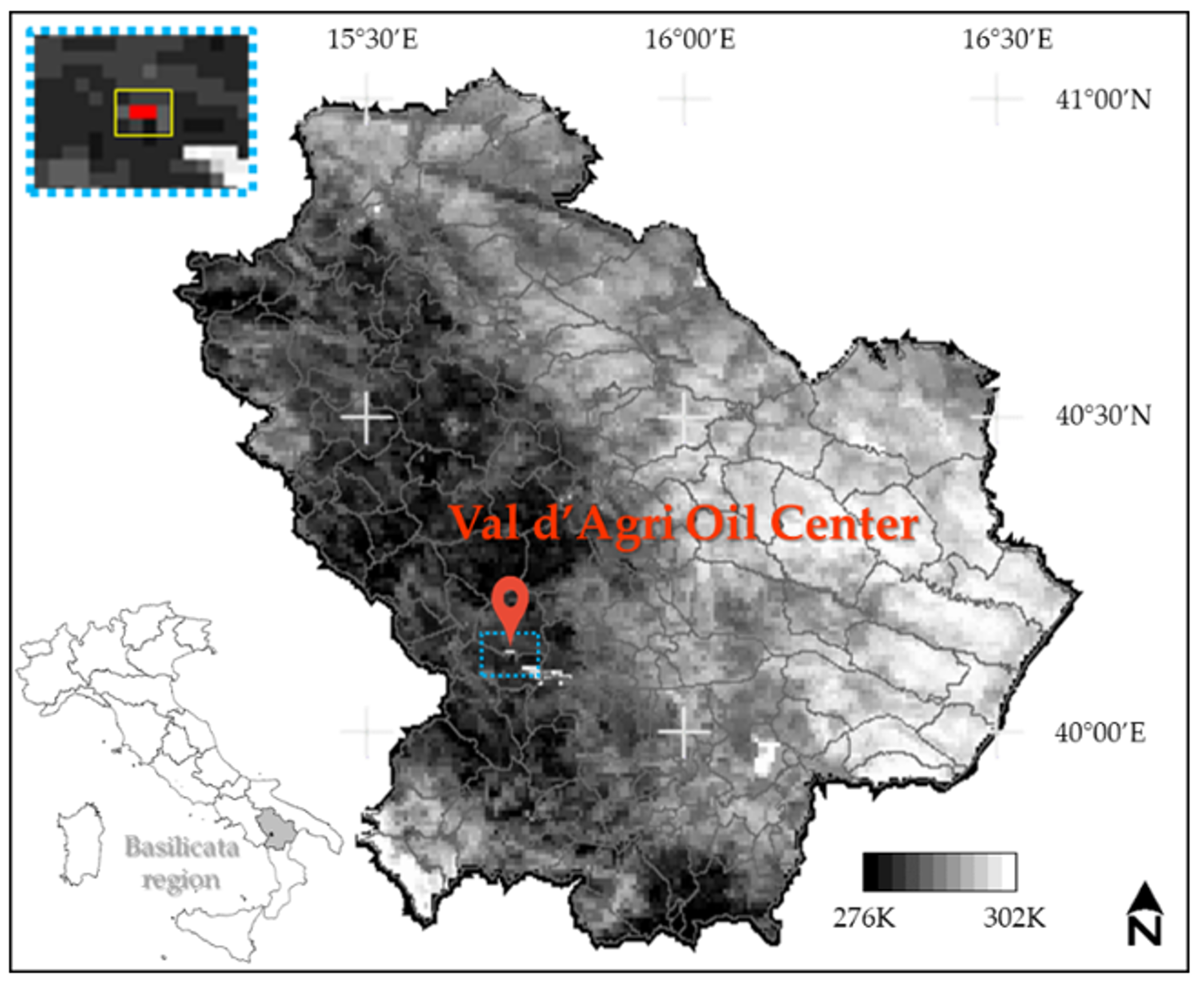
2. The Region of Interest

Basilicata region hosts the biggest onshore oil reservoir in Western Europe, which supplies over 10% of the Italian oil requirement. The oil is extracted from 24 wells that are currently in production in the Val d’Agri Concession (ENI 61%, Shell 39%), and then piped to the COVA in Viggiano (Figure 1) for its first treatment and sent through a pipeline to the Taranto refinery [46]. Currently, the COVA is the main onshore oil source in Italy (producing 77% of the national amount) by also supplying about half of the total gas production [47,48]. The Italian Ministry of Economic Development provides data on oil (in kg) and gas (in standard cubic meters, Sm³) production for the Val d’Agri Concession from 2004 to 2019 [48]. According to the last update of 23 November 2019, in the latest 15 years, the COVA produced a total of 55.00 million tons of oil and 17.43 billion Sm³ of associated gas (average annual value of 3.67 million tons and 1.16 billion Sm³, respectively) [48].

The COVA is the region of interest (ROI) in this study, namely the area within the yellow box shown in Figure 1, which makes it interesting for at least two main reasons.

First, it is located in an urbanized area, where inhabitants have been always worried about the plant potential impact on the health and ecosystem. Second, although it is inside an area of 100 km², with a dense environmental monitoring network (8 monitoring points/km²) [49], continuous information on the level of GF emissions released by this site (e.g., mass of GHGs, both CO₂ and CH₄, emissions as well as volumes of gas flared) are missing. The last “ground-truth” estimates about COVA GF provided by ENI date back to 2014 for both the volumes of gas sent to flaring (decreasing from 19.28 MSm³ in 2009 to 6.60 in 2014) and the CO₂ emissions from the treatment process and combustion activities (very stable around a mean value of 460 Mtons/year) [49,50,51]. Data on CO₂ emissions by gas flaring are limited to 2009-2011, when they represent less than 25% of the total [50]. This issue has pushed the local scientific community to bridge this gap by using satellite observing systems.

As anticipated in the introduction, the first satellite-based analysis of the COVA has been carried out by Reference [32] using MODIS data at 1 km of spatial resolution. In this paper, VIIRS data, with an improved spatial footprint of 750 m, have been exploited. The whole plant, whose size is 181.850 m² [47], spans more than two VIIRS 750 m pixels (Figure 1), with the gas flare system covering an area of ~800m². Such an area can be considered as a sub-pixel hot source, where the gas flaring phenomenon is managed through high level technologies allowing us to recover (and re-use for industrial and civil purposes) that most of the gas is carried out by the oil treatment [49]. In normal conditions, the torch burns a minimum amount of natural gas (soft gas), which feeds an almost invisible pilot flame. The volumes of gas flared by COVA are negligible when compared to most of worldwide upstream sites. For example, according to VNF estimates, in 2018, COVA flared 0.000907 BCM, while a Nigerian and Algerian upstream plant burned-off amounts 40-50 times greater (0.0037 and 0.044 BCM, mean value computed over the VNF detected sites, https://viirs.skytruth.org/apps/heatmap/flarevolume.html#).

3. Data

3.1. Satellite Data

Nighttime data acquired over COVA in the temporal range 1 January 2015 - 30 September 2019 by VIIRS sensors aboard Suomi-NPP (since October 2012) and JPSS-1 (since November 2017) satellites were collected and processed. The dataset includes images downloaded from the NOAA website (https://www.bou.class.noaa.gov/saa/products/welcome) as well as directly acquired by the receiving station installed at IMAA–CNR (Institute of Methodologies for Environmental Analysis - National Research Council), in Tito Scalo (Italy). 2.808 nighttime acquisitions were collected, with 2018 and 2019 representing 60% of the total, for the concurrent presence of both satellites. The VIIRS “Moderate” spatial resolution bands M07, M08, M10, M11, M12, M13, M14, M15, and M16 were selected to detect and characterize the COVA gas flare (

Table 1. Bands used.

	M07	M08	M10	M11	M12	M13	M14	M15	M16
Central wavelength [μm]	0.865	1.24	1.61	2.25	3.7	4.05	8.55	10.763	12.013
Band explanation	Near Infrared	Shortwave Infrared	Shortwave Infrared	Shortwave Infrared	Medium Infrared	Medium Infrared	Longwave Infrared	Longwave Infrared	Longwave Infrared
Processed data format	RD1	RD	RD	RD	RD/BT2	RD	RD	RD/BT	RD/BT

¹RD = Radiance. ²BT = Brightness Temperature.

). For the purposes of the study and the method applied, data were calibrated both as radiances (RD, W/(m²sr·µm)) and brightness temperatures (BT, K) values.

Starting from the Sensor Data Records (SDR), a portion centered over Italy (1800P x 1600L) re-projected in WGS84 Lat-Long projection, was produced for each of the VIIRS data included in the collected dataset. The ROI is a subset of this large area, corresponding to a box 4x3 (yellow box in Figure 1), where the COVA, in red, occupies the two central pixels (1386P – 1042L: Lat 40°18’34.20” N – Long 15°53’54.60” E, 1387P – 1042L: Lat 40°18’34.20” N – Long 15°54’19.80” E).

3.2. Ancillary Data

The ancillary data used in this study to assess the performances of the VIIRS-based RST-FLARE configuration in identifying hotspots at COVA were downloaded, as KML files, from the VIIRS Nightfire (VNF) “Nighttime Detection and Characterization of Combustion Sources” database, publicly available through the NCEI-EOG (National Centers for Environmental Information-Earth Observation Group) website (https://ngdc.noaa.gov/eog/viirs/download_viirs_fire.html). Two versions of the VNF algorithm are currently online, based on VIIRS observations provided by both CLASS (Comprehensive Large Array-data Stewardship System) and GRAVITE (Government Resource for Algorithm Verification, Independent Test, and Evaluation) portals. They mainly differ for the use of M11 in detecting combustion source, added in the latest version of VNF [52], since December 2017.

The VNF outputs cover the period from 31 March 2012 to 8 October 2019. The radiant heat (MW), temperature (K), and source footprint (m²) of the IR emitter are computed by a single (or dual) Planck curve fitting, depending on the number of bands (single, near-infrared - NIR or short-wave infrared - SWIR or multi-band, only in the MWIR or NIR/SWIR + MWIR) where the pixel is flagged as a combustion source [52]. The algorithm is able to detect combustion sources with temperature spanning from 400 K up to over 2500 K. The Planck curve fitting fails when hotspots are detected only in M10 (or M11). These cases, corresponding to dim sources, are designated as “non-conforming detections” (NCD).

The outputs (both hotspots, HS and NCD) provided by VNF for the COVA in the investigated temporal range are detailed in

Table 2. Detections over COVA in years 2015-2019.

Algorithm	Detection Type	2015	2016	2017	2018	2019	TOTAL
VNF	# Hotspots (HS)	10	4	5	35	49	103
	Non-conforming Detections (NCD)	10	16	18	100	116	260
	TOTAL	20	20	23	135	165	363

. In this work, the number of hotspots is the number of days in the same year, when the algorithm identifies one or more thermal anomalies over COVA. Hence, the real number of hotspots can be greater (or equal) than the days counted.

For the assessment of the VIIRS-based RST-FLARE outcomes, information provided by ENI through the three technical reports, referred to years 2012-2014, were exploited [49,50,51]. In addition, since 2016, a website dedicated by ENI to its role and activities in Basilicata (named “Eni in Basilicata”) was set up (https://www.eni.com/eni-basilicata/chi-siamo.page). The “News” section (https://www.eni.com/eni-basilicata/news/2019-elenco-news.page) collects all relevant events concerning the COVA from 2016 to date (the page is daily updated). For the purpose of this study,

Table 3. Significant periods of the COVA stop (source: “ENI in Basilicata” website).

	2015	2016	2017	2018
Time interval (reason)	27/01 – 06/02 (general plant shutdown)	20/02 – 26/02 (gas pipeline works) 16/04 – 12/08 (judicial seizure) 21/11 – 6/12 (flare system maintenance)	18/04 – 18/07 (political decision)	02/07 – 31/07 (ordinary maintenance work)
Total stop-days	11	142	91	30

lists the official long stop-periods (time interval and total days in the year) of the plant as well as the reasons of these interruptions (in the round brackets), used for the interpretation of results.

4. The Methods

A series of preliminary analyses were carried out to characterize the investigated site from a spectral point of view as well as to select the most suitable VIIRS bands to implement the RST-FLARE algorithm.

4.1. Temperatures Computed for COVA by VNF

First, the COVA site behavior in terms of temperature variation was assessed by exploiting the VNF outputs.

In detail, the temperature computed for the 103 hotspots detected over COVA by VNF between 1 January 2015 and 30 September 2019 (Figure 2) revealed that COVA exhibits a temperature lower than 1500 K in most cases (>70%). Temperature exceeds 1800 K only in one case (T=1878K on 4 August 2015 at 00.46GMT). The range 1300-1550 K was defined by Reference [14] as the crossover zone between temperatures recorded for gas flares and biomass burning by providing the first indication that COVA thermal emission can be seen both at SWIR and MWIR wavelengths.

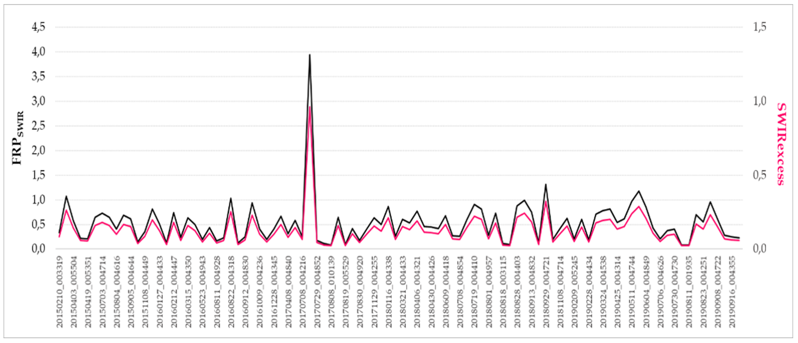
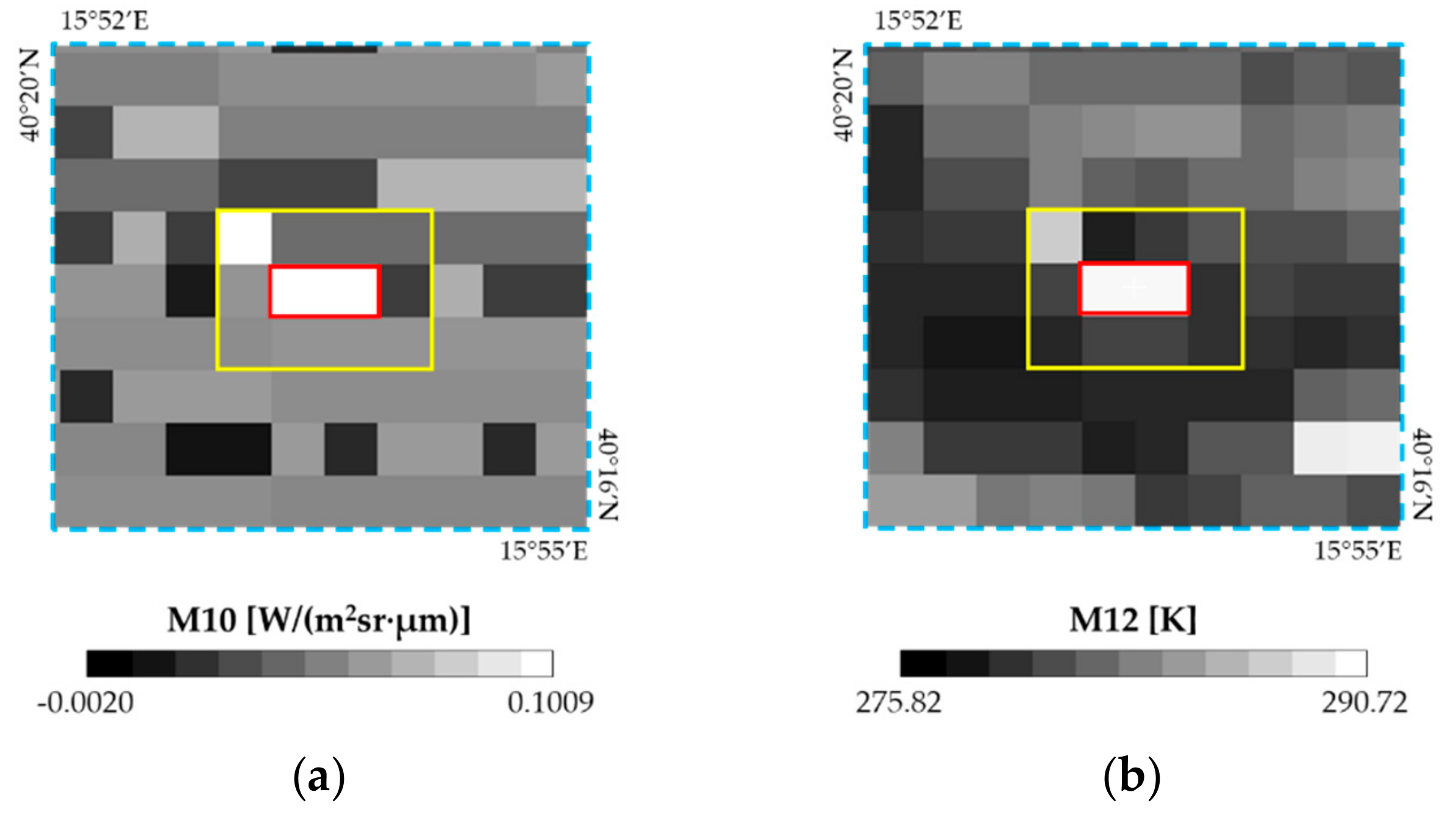
4.2. M10/M12 Radiances

Another test was carried out in order to confirm the peculiar COVA spectral behavior. According to Reference [20], the radiances ratio M10/M12 should range between 2.5-5.5 for gas flares at 1600–2200 K and 0–1.2 for landscape fires at 650–1330 K.

To assess such a behavior, 1.489 clear data (i.e., no cloudy pixels detected applying the method described in Section 4.4) for one of the two site-affected pixels (1386P–1042L) were analyzed in the above mentioned temporal period and compared to an “unperturbed” pixel very close to the site (1378P–1040L, Lat 40°19’24.60”N–Long 15°50’33.00”E), but far enough to be not thermally perturbed by COVA activity and not occupying any industrial activity (Figure 3).

The different behavior in terms of the M10/M12 ratio between the two sites is evident with the unperturbed pixel showing a value at around 0.02. The COVA is characterized by the ratio at least three times higher than the unperturbed pixel, but always below 1, except in one case, when it reaches the value of 2.205 (18 July 2017, at 00.55 GMT), which confirms the hybrid behavior of COVA concerning its thermal emission. “Hybrid” is meant in terms of the spectral behavior of COVA in both MIR and SWIR regions. This is further confirmed by looking at the signal recorded in the MWIR band (x-axis of Figure 3). COVA seems to show a very “warm” tail (BT_M12 > 293 K) with respect to the unperturbed pixel, which allows two main considerations. On one hand, such a result confirms that the COVA is almost an intermittent thermal emission source, On the other hand, due to its general low temperature, MWIR information can be profitably used to assess its behavior in support to the SWIR ones.

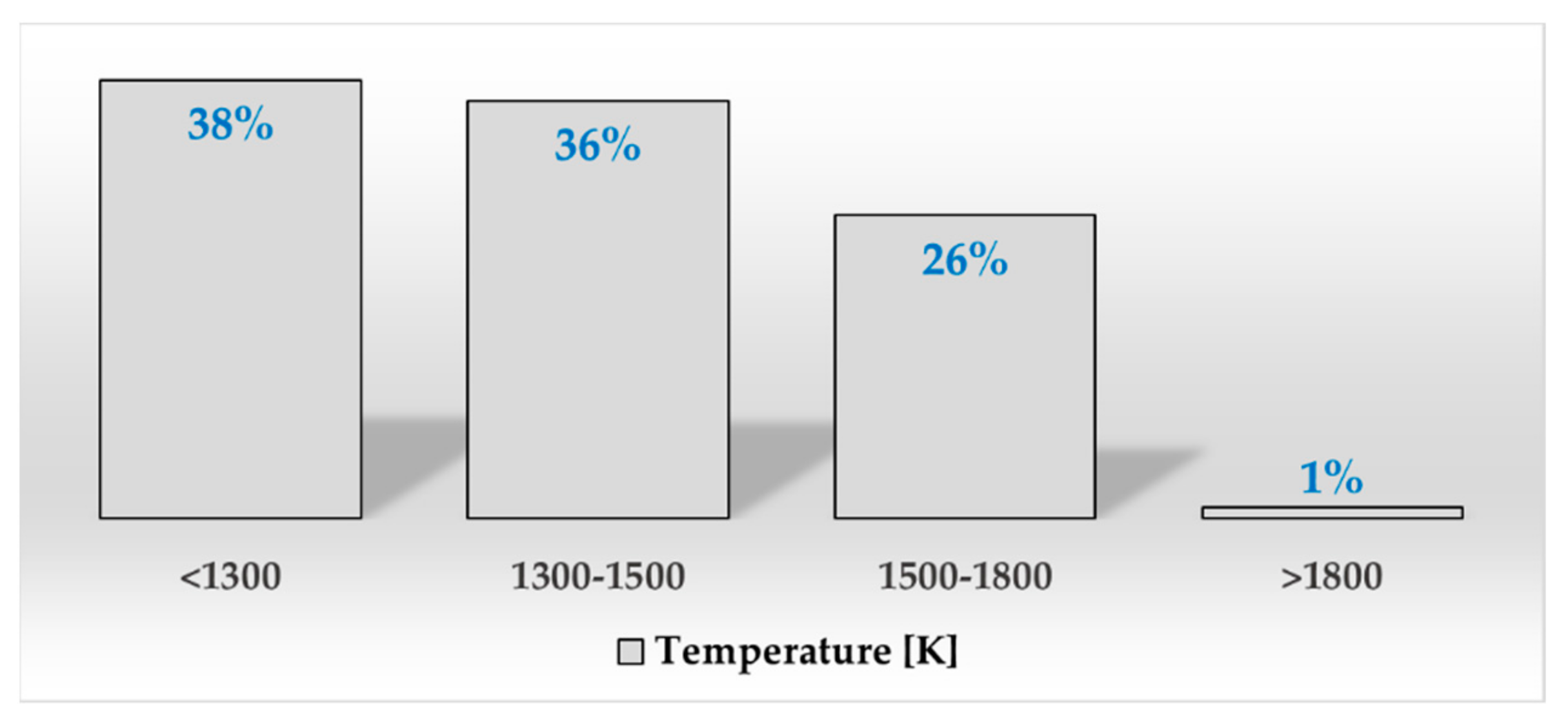
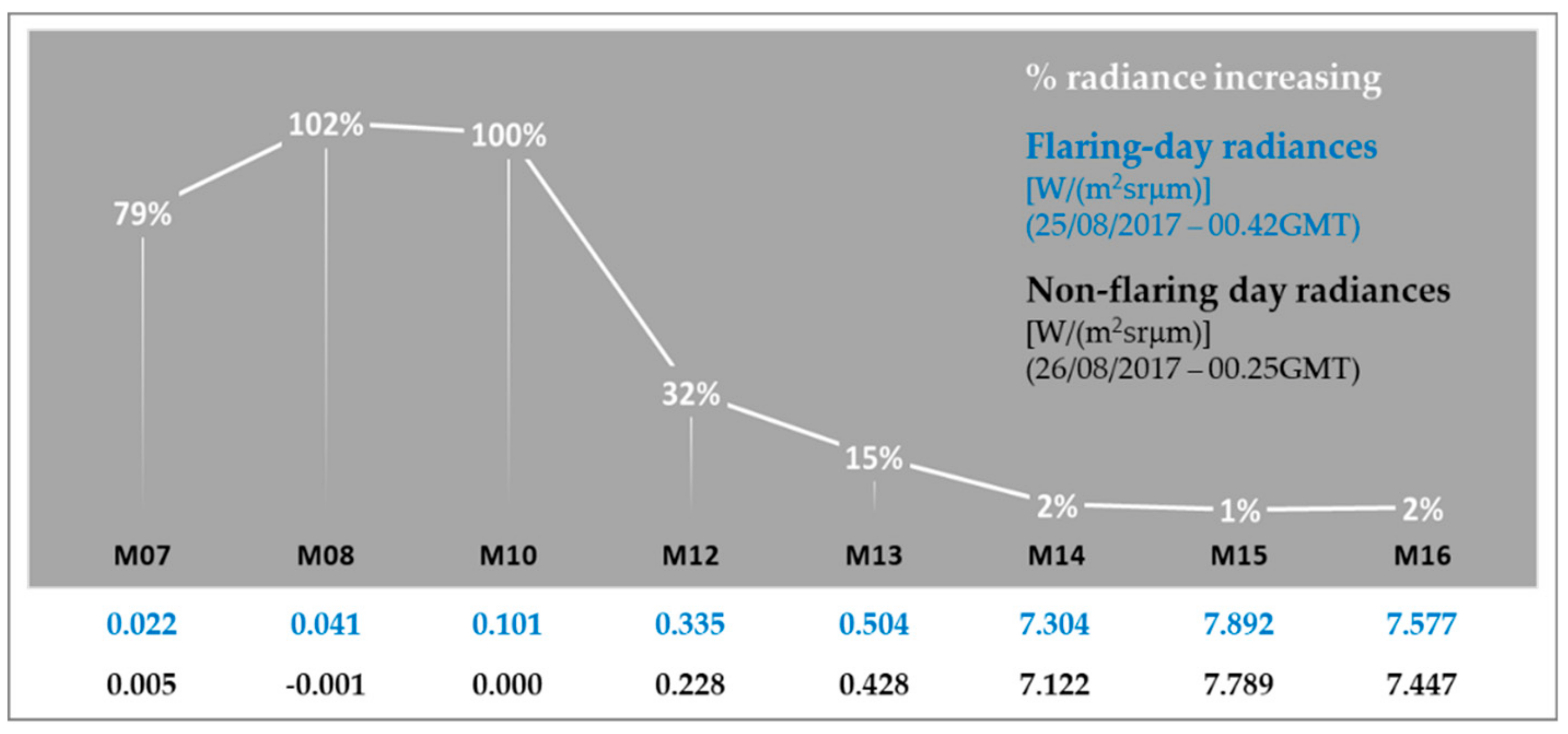
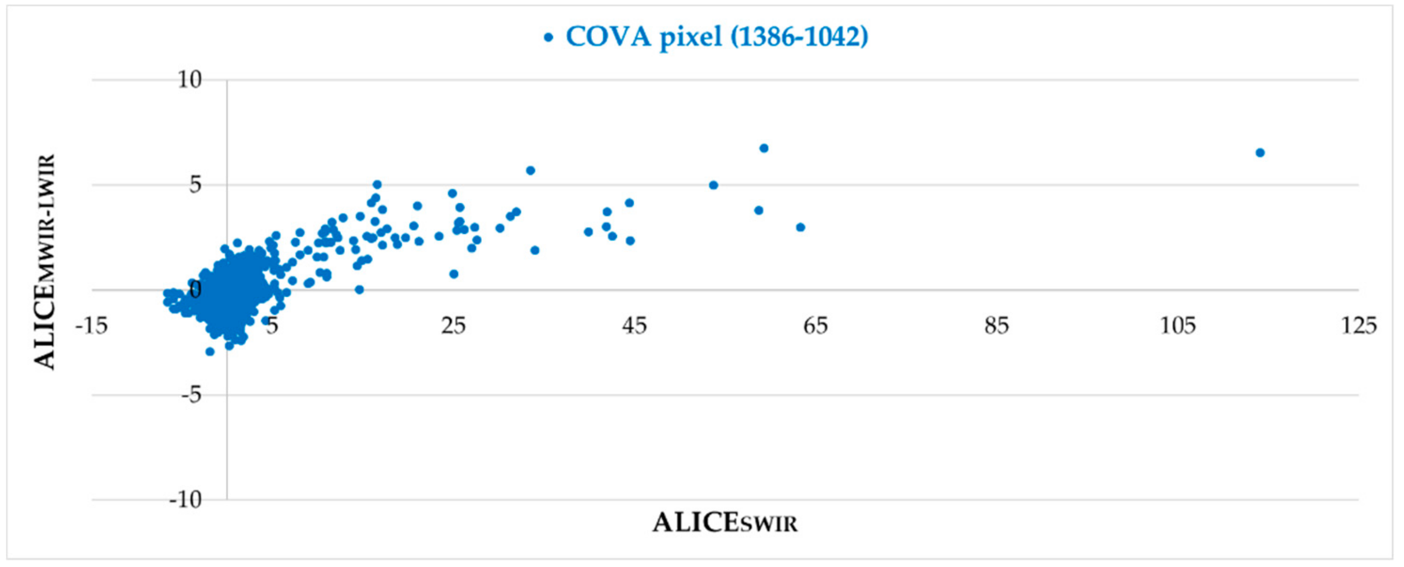
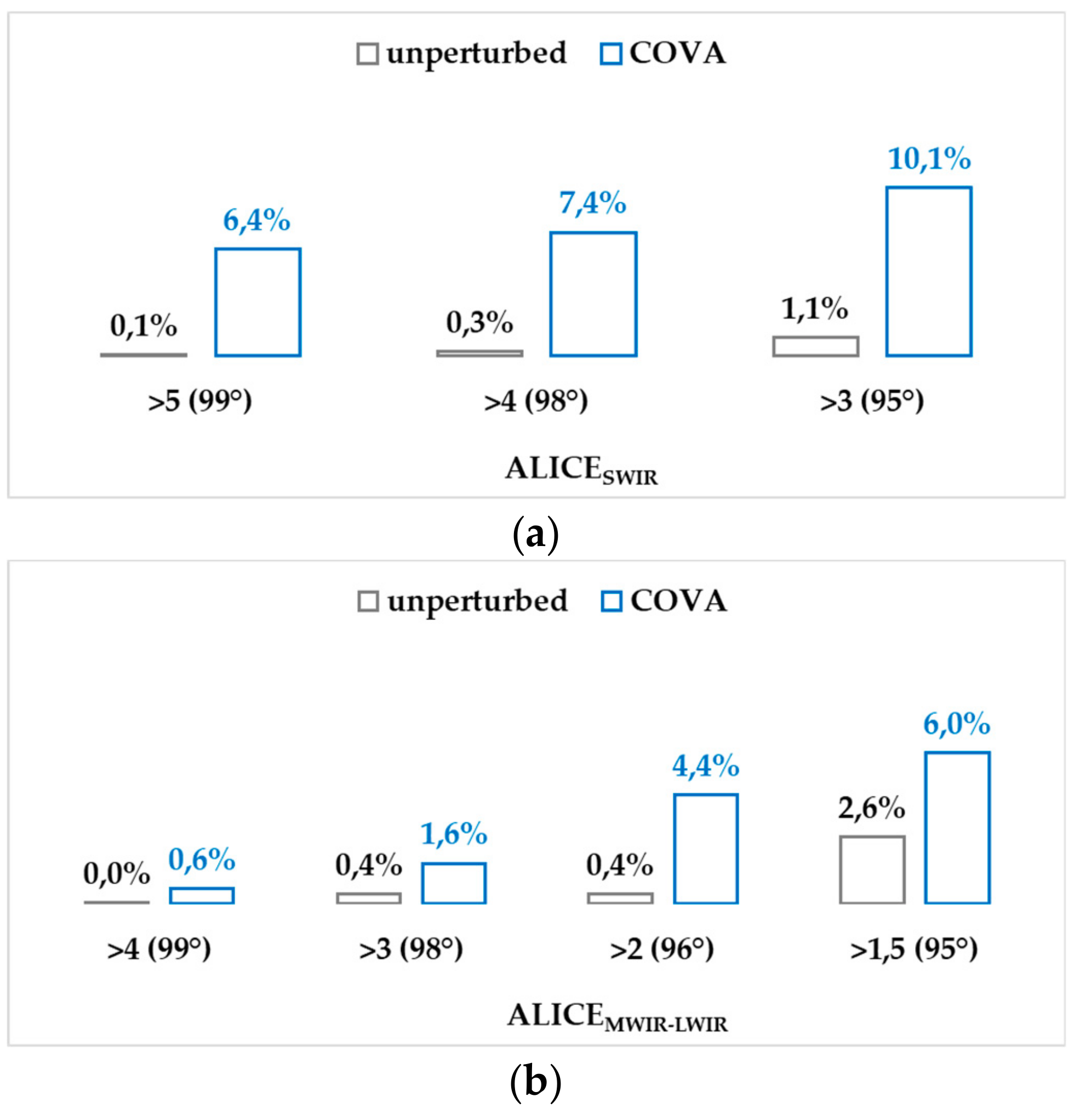
4.3. Spectral Characterization of COVA

Starting from the above considerations, two different VIIRS images were analyzed to better understand the spectral behavior of the COVA in the presence of a high level of thermal activity: the image of 25 August 2017, at 00.42GMT, characterized by clear evidence of a hotspot and the one on the next day (26 August 2017, at 00.25GMT) for which the pixel containing the gas flare does not show a significant thermal emission.

The radiances measured for the COVA pixel 1386P–1042L in these two images, in the spectral range from M07 to M16, are shown in Figure 4.

COVA shows two different thermal status in the two considered days. For an increasing plant temperature measured on 25 August 2017 (blue values in Figure 4), despite the one on 26 August (black values in Figure 4), the signal significantly raises at the lowest IR wavelengths (79%–100% at NIR-SWIR or M07-M10), moving to 32% and 2% from M12 to M14 and showing imperceptible variations in the LWIR (≤2% at M15, M16) (white line in Figure 4). This is an expected result by taking into account the output arising from the previous analyses. According to the Wien’s law, hot sources in the 1300-1550 temperature range have their emission peak in the NIR-SWIR spectral range with a smaller but still evident signal in the MWIR and any evident feature in the LWIR. Furthermore, combustion sources can be readily detected in the NIR and SWIR channels, dominated by background noise at night. Besides, using VIIRS short wavelength channels allows detecting smaller hot source areas across a broad range of temperatures [52]. In the MWIR, the higher signals can be associated to clouds, earth surface features, and combustion sources. In the LWIR, some of the largest flares shows faintly detectable signals [13,16].

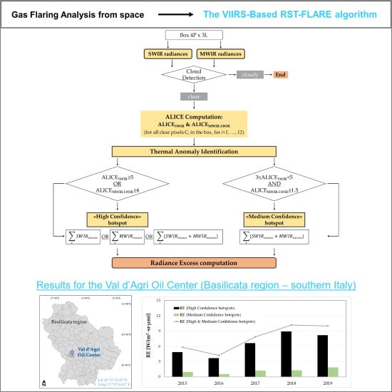
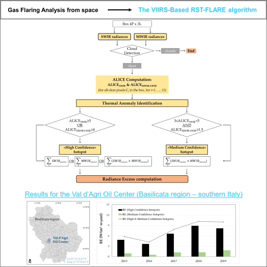
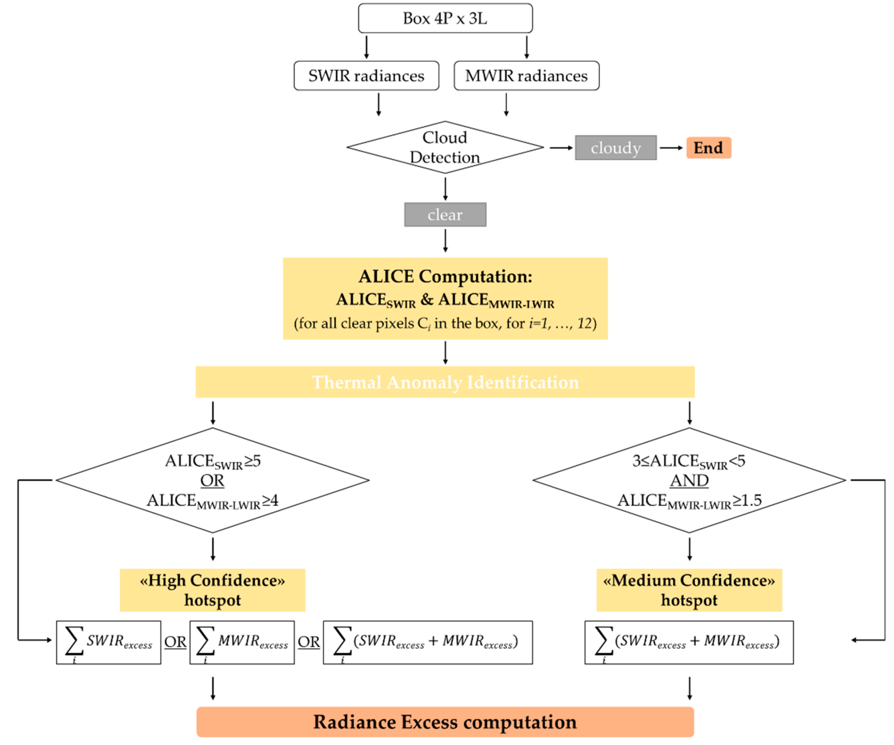
4.4. The VIIRS-Based RST-FLARE Algorithm

The strategy developed to identify thermal anomalies associated with gas flaring at COVA follows the general prescriptions of the RST-FLARE algorithm, previously implemented on multi temporal series of MODIS nighttime thermal data [32,33]. In this work, taking in mind the considerations shown in the previous paragraphs, the algorithm has been exported on VIIRS nighttime bands and the procedure was slightly modified (Figure 5). The main differences with the MODIS version rely on two aspects. The new configuration, in fact, i) works on a box 4 × 3 around the two COVA pixels (yellow box in Figure 1) and ii) takes into account the SWIR radiances in the same box to identify hotspots. The choice to consider a box instead of the two COVA-affected pixels (as done for MODIS) arose from the following considerations: i) residuals navigation errors may affect the hotspot detection, ii) when gas flares are observed at high satellite zenith angles, they result in larger source areas, which perturb more pixels [14]. The SWIR contribution has been included in order to improve the performances of RST-FLARE in detecting thermal anomalies and quantifying their radiant/emissive power.

The starting point of RST-FLARE is the collection of multi-year time series of satellite images over the region of interest, for defining, at a pixel level, the behavior of the signal under investigation in specific observational conditions [42,43,44]. To this aim, data are grouped on a monthly temporal scale. Only cloud-free pixels are used and marked as valid. Cloudy pixels are detected by applying the OCA approach (the One-channel Cloud-detection Approach) [53,54], using the LWIR brightness temperatures (i.e., VIIRS M16 channel). SWIR to MWIR signals measured in the COVA box were analyzed by following the scheme shown in Figure 5.

Following the previously shown VIIRS-based analyses of the thermal behavior of COVA pixels, two ALICE (Absolutely Llocal Index of Change of the Environment) indices are computed for each clear pixel in the box to identify, among the signals under investigation (SWIR and MWIR-LWIR), the ones associable with the presence of hotspots at the COVA site:

ALICE_SWIR = (SWIR_i - μ_SWIR,i)/σ_SWIR,i

(1)

ALICE_MWIR-LWIR = [(MWIR_i-LWIR_i) - μ_{MWIR,i-LWIR,i}]/σ_{MWIR,i-LWIR,i}

(2)

The ALICE index is assumed as a standardized variable characterized by a Gaussian behavior (i.e., with mean equal to zero and standard deviation equal to 1). This means that the probability of occurrence of values higher than 2 standard deviations is less than 2.28% and it becomes lower than 0.13% for values higher than 3. For each signal (SWIR or MWIR-LWIR), the normal behavior of each pixel is expressed by a mean value (μ) and a normal variability (σ). Hotspots are defined as pixels whose signal exceed a pre-defined confidence level value.

For the analyzed phenomenon, high values of both ALICEs are expected for the pixel at position i in the 4x3 box when COVA produces high thermal emissions. These thermal anomalies should indicate the occurrence of major fluctuations in the COVA combustion operations and/or to the gas flaring in emergency conditions.

The confidence levels were identified for each of the two investigated signals by a percentile analysis applied to the two-time series of ALICE indices computed on COVA pixels from 1 January 2015 to 30 September 2019 (Figure 6).

The choice of the above-mentioned confidence level also depends on the error committed in correctly identifying hotspots. Such an error is quantified by the percentage of thermal anomalies detected over the unperturbed pixel previously analyzed, characterized by the absence of any industrial activities, and by applying a specific threshold to the ALICE_SWIR and ALICE_MWIR-LWIR values (Figure 7).

By combining information acquired by the analysis of data in Figure 6 and Figure 7, two confidence levels were chosen and thermal anomalies were classified into two groups: “High Confidence” (HC) and “Medium Confidence” (MC) hotspots.

Using the 99th percentile, a threshold of 5 for the ALICE_SWIR and 4 for the ALICE_MWIR-LWIR was found (Figure 6), which implies that, in both cases, an error of 0.1% was found (Figure 7). Therefore, at these levels, HC hotspots are identified as:

ALICE_SWIR ≥ 5 or ALICE_MWIR-LWIR ≥ 4

(3)

Considering the 95th percentile, MC hotspots are discriminated at a detection level between 3 and 5 for the ALICE_SWIR and greater than 1.5 for the ALICE_MWIR-LWIR, respectively (Figure 6).

3 ≤ ALICE_SWIR < 5 and ALICE_MWIR-LWIR ≥ 1.5

(4)

At this level, a maximum error of 2.6% is committed (Figure 7).

Once the hotspot is detected within the box on a specific day, its thermal characterization is performed. Following Reference [33], the emissive power of the heat source is expressed in terms of radiance excess (RE), which corresponds to the deviation of the M10 or/and M12 radiances, depending on the way (i.e., level of confidence, HC or MC) the hotspot was identified with respect to a pre-defined background value. For each day, a daily RE is calculated as the sum of all REs computed for the hotspots detected within the 4x3 box. The daily records are then aggregated on an annual scale.

In detail, for HC hotspots, RE can be equal to:

$$\mathrm{REy}\left(\mathrm{SWIR}\right)={{\displaystyle \sum }}_{\mathrm{i},\mathrm{y}}(\mathrm{M}10\mathrm{hotspot}-<\mathrm{M}10\mathrm{bg}>) {\mathsf{\alpha }}_{\mathrm{y}} [\mathrm{W}/({\mathrm{m}}^2\mathrm{sr}·\mu \mathrm{m})]$$

(5)

$$\mathrm{REy}\left(\mathrm{MWIR}\right)={{\displaystyle \sum }}_{\mathrm{i},\mathrm{y}}(\mathrm{M}12\mathrm{hotspot}-<\mathrm{M}12\mathrm{bg}>){\mathsf{\alpha }}_{\mathrm{y}} [\mathrm{W}/({\mathrm{m}}^2\mathrm{sr}·\mu \mathrm{m})]$$

(6)

$$\mathrm{REy}=\left[\mathrm{REy}\left(\mathrm{SWIR}\right)+\mathrm{REy}\left(\mathrm{MWIR}\right)\right]{\mathsf{\alpha }}_{\mathrm{y}} [\mathrm{W}/({\mathrm{m}}^2\mathrm{sr}·\mu \mathrm{m}\left)\right]$$

(7)

where:

• y refers to each of the investigated years in the 2015-2019 period,
• i refers to each hotspot identified in the box (for i=1, …, 12),
• M10_hotspot (M12_hotspot) is the radiance measured in the VIIRS band M10 (M12) for the hotspot i,
• <M10_bg> (<M12_bg>), referring to the background, is equal to the spatial mean of the temporal average μ_M10(x,y) (μ_M12(x,y)) of the first neighboring pixels around the box,
• α_y is a coefficient which weighs the variability, between years, in sampling and cloud cover. It is computed as the ratio between the clear and total images. To take into account its variability in the considered temporal range, it has been normalized with respect to its maximum value computed within 5 years (α_y,max= 0.59).

For MC hotspots, RE corresponds to the sum of RE_y(SWIR) and RE_y(MWIR) (5).

Lastly, a short comment on the excess of radiance (RE), the metric used to quantify the radiative power of the gas flare pixel. RE is based on M10 and M12 signals, similar to the ones used in the methods suggested by Reference [20], i.e., the SWIR and MIR-Radiance methods, for gas flaring estimation. Both methods quantify the radiant power of a gas flare by computing the Fire Radiative Power (FRP) using M10 and M13 radiances, respectively (i.e., FRP_SWIR or FRP_MIR). The COVA peculiar behavior does not allow the use of the FRP formulas to accurately assess its radiant heat. On one side, the hybrid behavior of COVA, when generating anomalous (i.e., hotter than background) radiances not only at SWIR wavelengths but even (and, in some cases, exclusively) in MWIR spectral region, requires both responses to be taken into account. This is why the radiance excess, as the sum of both SWIR and MWIR contributions, should be the most appropriate way to characterize such a hot source. Additionally, using the MIR-Radiance method for considering the COVA MWIR contribution could not be proper for this kind of site since the M13 band (the one used in Reference [20] and for which the FRP coefficient is available) is less sensitive than M12 to GF-related hotspots at COVA (see Figure 2). For these reasons, it is expected the COVA radiant heat estimates carried out using only the SWIR-Radiance method or both Radiance methods will be affected by uncertainty because: i) not including the MWIR contribution (in the first case) or ii) not using the most suitable MWIR band for COVA gas flare (in the second one).

A direct comparison of SWIR_excess (in W/(m²·sr·µm)) and the FRP_SWIR values (in MW) both computed for the COVA pixel 1386P – 1042L for all useful data in years 2015-2019 showed a linear correlation coefficient (R) of 0.99 between the two temporal trends (Figure 8). This analysis demonstrated the high consistency of our estimates.

5. Results

This section provides a concise and precise description of the experimental results and their interpretation, together with a comparison with VNF products. A linear equation aimed at estimating the COVA radiant heat from its radiance excess has been developed.

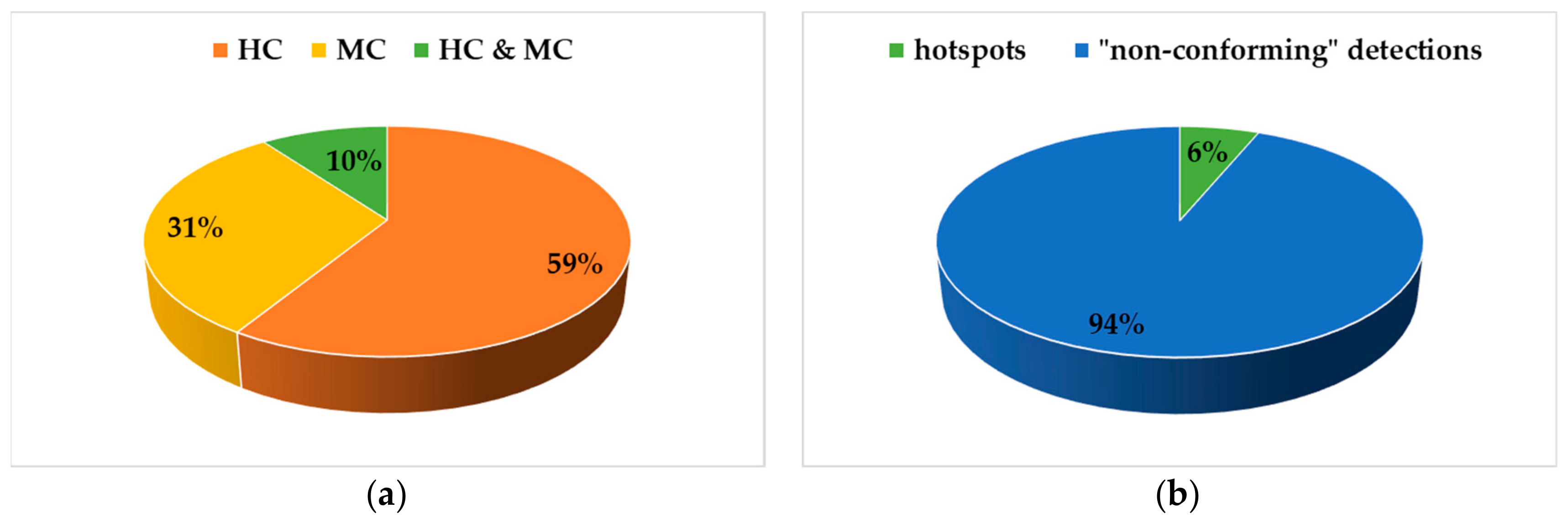
5.1. VIIRS-Based RST-FLARE Outputs

The VIIRS-based RST-FLARE outputs are shown below.

The developed algorithm identifies 275 hotspots from 2015 to 2019 (as the sum of the numbers in the last line in

Table 4. The VIIRS-based RST-FLARE hotspots detections, divided between HC and MC levels. The common dates with both HC and MC hotspots are in the third line.

	2015	2016	2017	2018	2019
# HC hotspots	23	28	28	55	58
# MC hotspots	11	5	9	10	27
HC and MC	4	2	6	9	/
TOTAL	38	35	43	74	85

), classified as High (HC) and Medium Confidence (MC) levels. The line “HC and MC” in Table 4 counts the days when RST-FLARE identified both HC and MC hotspots for pixels occupying different positions in the box matrix.

The number of days with hotspots is very stable between 2015 and 2017 (moving from 38 to 43, Table 4), with increasing values in the two following years, 2018 and 2019, almost double when compared to the previous ones. This is very likely due to the launch of a second satellite (i.e., JPSS-1) hosting the VIIRS sensor onboard.

The annual radiance excess computed for the hotspots belonging to two separated datasets (i.e., HC and MC) as well as the total one, which consists of their sum, is depicted in Figure 9.

Focusing on the Radiance Excess trend in the five-years period (gray line in Figure 9), its minimum is observed in 2016. Then it increases up to 2018, while slightly decreasing in 2019 (~2%). It is interesting to note that in both graphs the inflection point is in 2016, which is the year with the longest stop of COVA activities, and lasted in a total of almost five months (see Table 3).

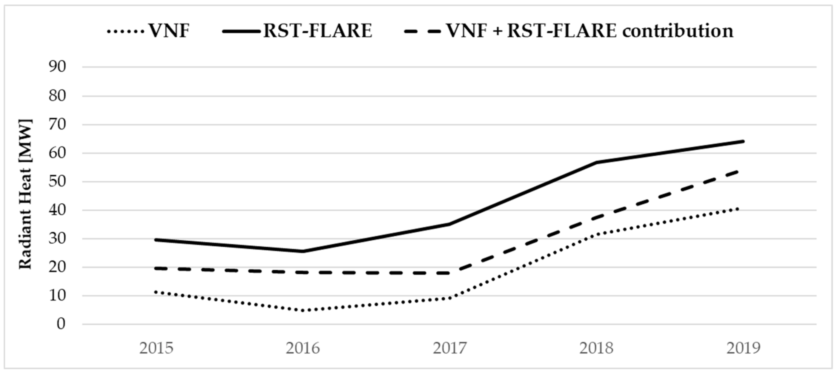
5.2. Comparison with VNF

The outputs provided by VIIRS-based RST-FLARE are tabulated in

Table 5. Summary and comparison between VNF and VIIRS-based RST-FLARE detections.

	Detection type	2015	2016	2017	2018	2019	TOTAL
VNF	HS + NCD	20	20	23	135	165	363
VIIRS-based RST-FLARE	TOTAL (HC& MC)	38	35	43	74	85	275
Match with VNF	(HC& MC) vs HS	10	4	5	30	41	90
	(HC& MC) vs NCD	9	16	12	9	20	66
	Total matches	19	20	17	39	61	156

by also displaying the comparison with VNF detections (already shown in Table 2).

The two datasets (first two lines in Table 5) are highly correlated (R=99%) in terms of temporal evolution along the considered period, with RST-FLARE detections almost doubling when compared to VNF between 2015 and 2017 and a turnaround in the following two years. This is mainly due to the additional use of M11 band in the VNF algorithm, which increased by 55% its performances in detecting combustion sources, even with a smaller size and lower temperatures [52].

A deeper investigation of the two outputs was conducted, focusing on the uncommon detections. The 119 RST-FLARE hotspots not detected by VNF (i.e., 275 – 156) are plotted in Figure 10a in terms of their distribution between the two levels of confidence (i.e., HC and MC) and the “mixed” hotspots (i.e., when they have been classified as both HC and MC). Figure 10b shows the 207 (i.e., 363-156) VNF hotspots, divided between hotspots and “non-conforming” detections, not identified by VIIRS-based RST-FLARE.

Most of VNF hotspots not identified by RST-FLARE are “non-conforming” detections (i.e., 94%). In 6% of cases (i.e., 13 hotspots), VNF identified hotspots over COVA. Two conditions might determine the RST-FLARE missing identifications compared to the VNF ones including the presence of clouds over the ROI and the values of ALICE indices below the selected confidence levels. A visual inspection of the M10 and M12 channels of all 13 imagery (5 in 2018 and 8 in 2019) confirmed that, although they were classified as cloudy by the OCA approach, hotspots are evident in the COVA box. This circumstance is typically observed in the case of very thin clouds that are not able to fully mask the signal coming from the surface but are still (and correctly) identified as cloudy days.

For a more quantitative comparison with VNF, the first analysis was devoted to investigate the temporal match of VIIRS-based RST-FLARE and VNF hotspots (HS), not considering the “non-conforming detections” (NCD) (Figure 11). Furthermore, 90 correspondences (same day and same hour of acquisition) were detected for COVA by both algorithms between 2015 and 2019 (see Table 5). Their characterization, along the considered period, in terms of RE and RH is shown in Figure 11, which confirms a satisfactory agreement between these two parameters (R=90%).

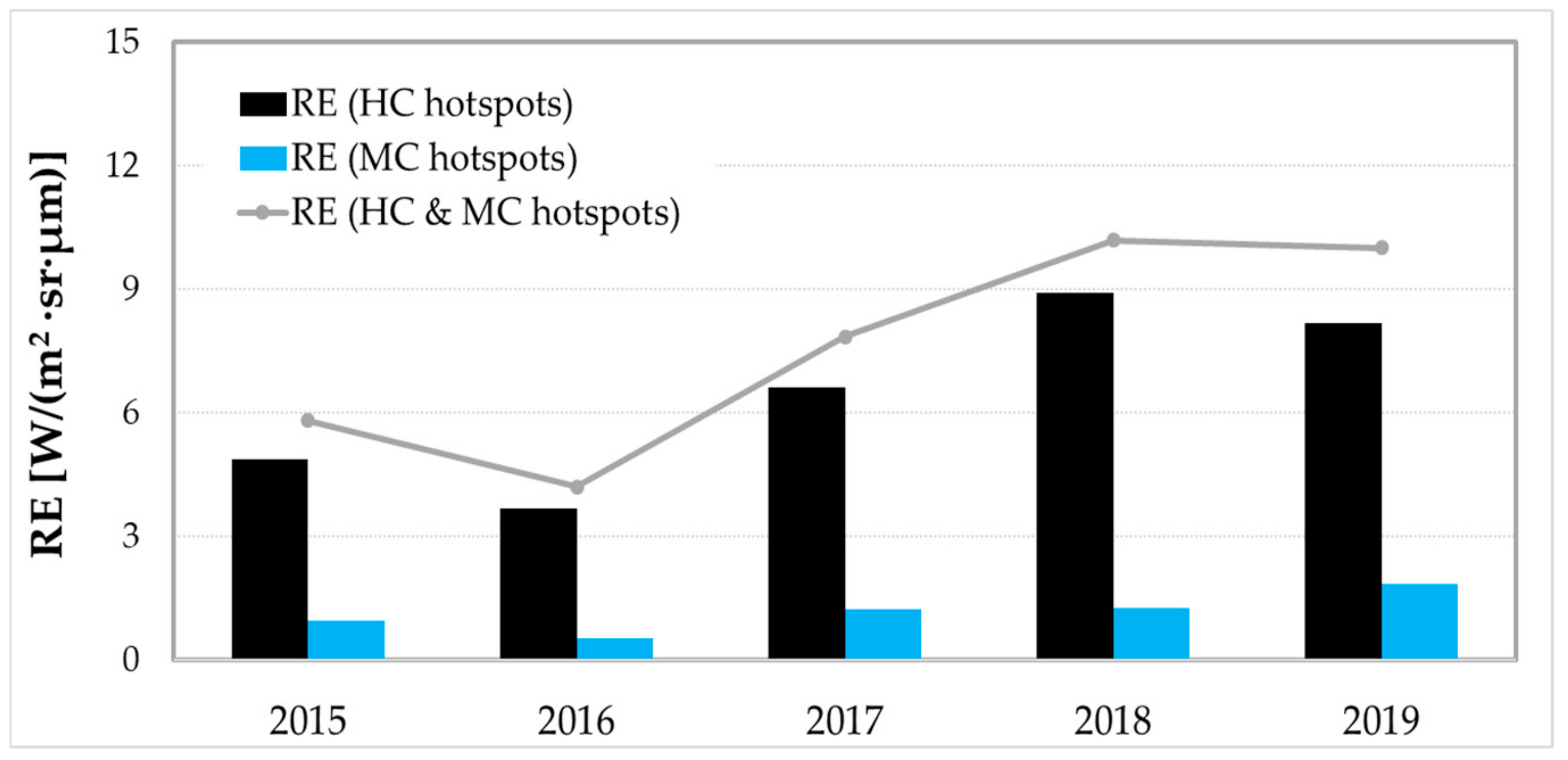
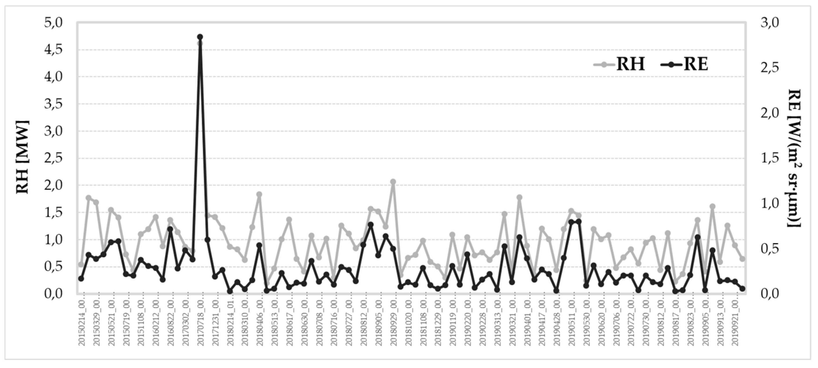
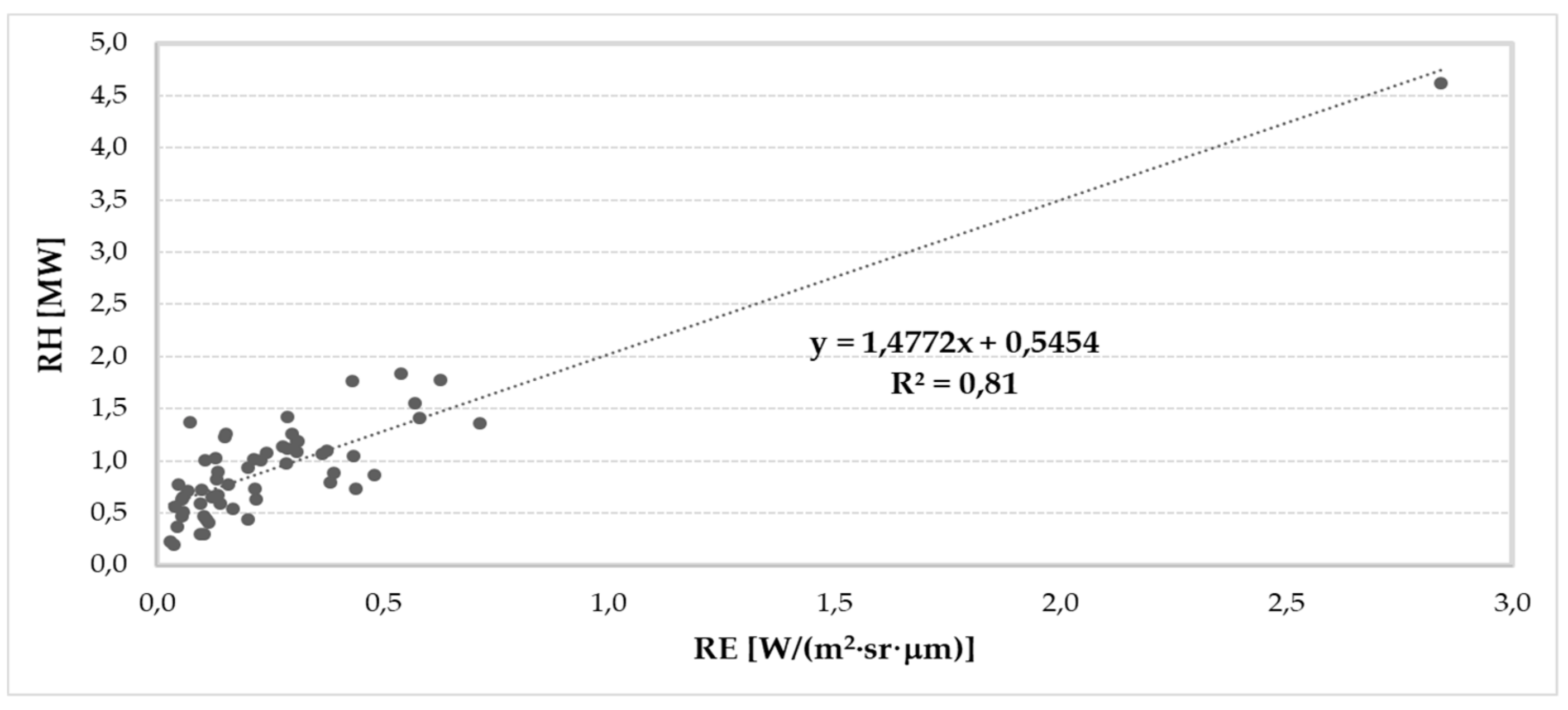
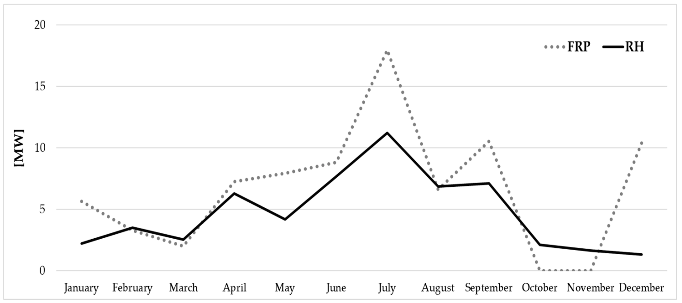
5.3. Radiant Heat Estimation

The high consistency between the two metrics allowed for developing a linear equation able to estimate RH using the corresponding RE for each detected RST-FLARE hotspot. This is a site-specific model developed to better characterize the COVA behavior using both SWIR and MWIR responses. To this aim, the 90 common detections were split into two different datasets: one (i.e., 60 records, equal to 67%, randomly selected among the 90 matchings) was used to calibrate a linear regression model aimed at computing the radiant heat from the radiant excess (R² = 0.81, Figure 12).

The other dataset, containing the remaining 30 detections, was exploited to validate the developed model (R² = 0.56, bias = 0.031, NRMSE (normalized root mean square error) = 17%). The equation in Figure 12 was then used to estimate RH even for the “non-conforming” VNF detections (i.e., 66 data). In fact, for these detections, the VNF scheme is not able to compute RH and, then, their indirect characterization, exploiting the RE provided by the RST-FLARE algorithm, can be particularly useful in these cases.

Figure 13 shows the radiant heat computed for COVA, for each year from 2015 to 2019, by RST-FLARE (for a total of 275 hotspots, black line in Figure 13), and VNF (for its 103 hotspots, black dotted line in Figure 13).

The RST-FLARE scheme allowed recovering 66 VNF “non-conforming” detections (25% of its total) that strongly increased the VNF RH estimates of the COVA plant (black dashed line in Figure 13).

This information can be used to update RH estimates in view of acquiring in-situ data about COVA volume emissions that can be used to develop a model aimed at inferring emitted volumes starting from radiant heat estimates.

6. Discussion

The VIIRS-based RST-FLARE algorithm developed in this work is able to provide the radiant heat RH (MW) of the COVA gas flare for each detected hotspot. It is derived from the radiance excess, RE, which adds up the VIIRS SWIR and MWIR contributions (at 1.61 and 3.7 μm, respectively) in case a thermal anomaly occurs at the COVA plant. The comparison with VNF estimates in the investigated temporal range (i.e., 2015-2019) widely demonstrated good agreement between the two independent products, especially in terms of their temporal trends. Moreover, the proposed model, when applied over the investigated source, seems capable of overcoming some limits of the VNF methodology in deriving RH estimates in the presence of lower level (i.e., “non-conforming detections”) thermal anomalies. In such a way, RST-FLARE-based RH estimates can complement VNF outputs, contributing to better characterize the COVA source in the time domain reliability of such products as well as their add-on value in improving VNF capability to quantify the radiant heat.

The proposed VIIRS-based algorithm represents a new configuration of the previous, MODIS-based, RST-FLARE technique. It has been proposed to: i) guarantee the continuity of gas flaring monitoring and investigation after the (possibly close) end of MODIS life, and ii) exploit the improved spatial and spectral resolutions of VIIRS with respect to MODIS. However, presently, the MODIS sensor is still operating very well and the related RST-FLARE configuration is routinely applied at COVA. Therefore, VIIRS-based findings can be also compared with the ones achieved by means of the original RST-FLARE configuration. The latter is using the FRP as the satellite metric aimed at computing the gas flare emissive power [32]. The VIIRS-based RH and MODIS-based FRP values, aggregated at an annual scale, in the temporal period 2015-2019, are shown in Figure 14. This figure highlights good agreement (R=88%) between the two metrics (with systematic higher FRP estimates) even though they are based on independent sensors data with different (spatial and spectral) features. Looking at the two curves in Figure 14, it is clear that they show a very similar behavior, with a minimum in 2016 and an increasing trend in the following years.

The inter-products comparison has been carried out at a monthly scale. As an example, the estimates provided for 2018 by RH and FRP are shown in Figure 15.

The high consistency of the two metrics is further confirmed (R=76%), especially in terms of their temporal trend (Figure 15), even though they provide different results in some months (e.g., December). The latter might be partially due to a cloud effect, which is expected to be more pronounced in the winter months. Figure 15 demonstrates the temporal consistency of the products, which clearly highlights even the possible add-on coming from the integration of two schemes in the thermal characterization of a gas flare. Focusing on October and November 2018, only VIIRS-based RST-FLARE is able to identify a hotspot at COVA (3 in October and 2 in November) and quantify their radiant heat. This is likely due to the better VIIRS spatial resolution as well as regarding the use of a SWIR channel (missed in MODIS nighttime imagery), particularly suitable for gas flaring analysis. To show an example, the M10 and M12 records measured in the COVA area on 8 November 2018, at 00.47 GMT, are shown in Figure 16 and are depicted in gray tones.

The two COVA affected pixels (red box in Figure 16) are the ones in the scene with the highest values in both SWIR and MWIR channels and clearly appear as highly radiant compared to the surrounding pixels.

All the above considerations suggest a higher performance to be expected from a multi-sensor RST-FLARE approach.

Future research studies will be addressed in two directions.

The MODIS-based RST-FLARE scheme is able to provide GF information for COVA since 2000, which characterizes this thermal source not only in terms of FRP but also in terms of gas volumes emitted into the atmosphere [32]. The portion of the MODIS-based configuration on the VIIRS IR Imagery bands (i.e., I4 and I5, centered at 3.74 and 11.45 μm, respectively) will be tested to guarantee the continuity of the provision of this type of information in view of assessing the possible improvements coming from the finer (i.e., 375 m versus 1000 m) spatial resolution of these data.

Furthermore, the possible contribution to COVA characterization coming from the usage of the M11 band (2.23-2.28 μm) will be investigated.

Lastly, due to the intrinsic independence of the RST approach from the local conditions, a further development will be the RST-FLARE implementation during daytime, to assess its performance in more difficult (i.e., in the presence of solar radiation) environmental conditions as well as to increase the sampling frequency and, consequently, the satellite-based monitoring capabilities of a gas flaring phenomenon.

7. Conclusions

In this work, an adapted version of the RST-FLARE algorithm for VIIRS data has been presented and results have been achieved by investigating the COVA oil and gas pre-treatment plant in Val d’Agri (Basilicata region, southern Italy), which have been shown and assessed for the period 2015-2019 including for a comparison with VNF (i.e., VIIRS Nightfire) records.

Findings confirm that RST-FLARE, originally designed and developed for MODIS mid-infrared data, can be properly ported on a different satellite/sensor system like the Suomi/NPP and JPSS-1 VIIRS SWIR and MWIR records.

Thermal anomalies detected over the COVA plant have been assessed by using independent VNF outputs, which confirms good agreement between the two procedures. A specific metric to quantify and characterize detected hotspots (i.e., Radiance Excess – RE) has been evaluated by investigating its relationship with an independent quantity, i.e., the Radiant Heat – RH, which is a standard output of the VNF technique. In addition, in this case, the two quantities have shown a very high correlation (R = 90%) by allowing RE to be used for quantitatively characterizing gas flare thermal sources. Lastly, the high RE-RH correlation allowed for designing a model capable of estimating RH values in cases when VNF is not able to provide any quantitative information (i.e., in correspondence of the “non-conforming detections”). This outcome would enable RST-FLARE as an additional source of information to be used for characterizing and quantifying gas flares, at least at a local scale, by complementing VNF outputs. The regression model converting RE in RH is site-specific being “ad hoc” developed for providing an accurate characterization of the COVA radiant heat to use in the next studies devoted to estimate COVA GF emissions. Its porting to other geographic areas and power plants requires data inherent to the investigated site for the coefficients’ calibration. The RST-FLARE algorithm, only based on satellite data for the RE, has a global applicability.

In perspective, since this more refined and complete information would contribute to better estimate of the quantity of gas volumes emitted into the atmosphere (in fact, as already largely demonstrated, the radiant power/heat of thermal sources is a proxy of emitted gas volumes), the potential add-on of RST-FLARE in this sense could be significant.

The demonstrated good consistency between the two RST-FLARE developed schemes, one based on nighttime MWIR MODIS channels and the other one based on SWIR and MWIR VIIRS acquisitions, further strengthen the potential of the proposed configuration in view of implementing a multi-sensor RST-FLARE strategy for the analysis of gas flaring sources and for assessing their environmental impacts.

References

1. Emam, E.A. Environmental Pollution and Measurement of Gas Flaring. Int. J. Sci. Res. Sci. Eng. Technol. 2016, 2, 252–262. [Google Scholar]
2. U.S. Department of Energy, Office of Oil and Natural Gas Office of Fossil Energy. Natural Gas Flaring and Venting: State and Federal Regulatory Overview, Trends, and Impacts; U.S. Department of Energy: Washington, DC, USA, 2019. [Google Scholar]
3. Soltanieh, M.; Zohrabian, A.; Gholipour, M.J.; Kalnay, E. A review of global gas flaring and venting and impact on the environment: Case study of Iran. Int. J. Greenh. Gas Control 2016, 49, 488–509. [Google Scholar] [CrossRef]
4. Nanok, J.K.; Onyango, C.O. A Socio-Economic and Environmental Analysis of the Effects of Oil Exploration on the Local Community in Lokichar, Turkana County, Kenya. Int. J. Manag. Econ. Soc. Sci. 2017, 6, 144–156. [Google Scholar]
5. Giwa, S.O.; Nwaokocha, C.N.; Kuye, S.I.; Adama, K.O. Gas flaring attendant impacts of criteria and particulate pollutants: A case of Niger Delta region of Nigeria. J. King Saud Univ. Eng. Sci. 2019, 31, 209–217. [Google Scholar] [CrossRef]
6. Global Gas Flaring Inches Higher for the First Time in Five Years. Available online: https://blogs.worldbank.org/opendata/global-gas-flaring-inches-higher-first-time-five-years (accessed on 3 February 2020).
7. Elvidge, C.D.; Bazilian, M.D.; Zhizhin, M.; Ghosh, T.; Baugh, K.E.; Hsu, F.-C. The potential role of natural gas flaring in meeting greenhouse gas mitigation targets. Energy Strategy Rev. 2018, 20, 156–162. [Google Scholar] [CrossRef]
8. Caseiro, A.; Gehrke, B.; Rücker, G.; Leimbach, D.; Kaiser, J.W. Gas flaring activity and black carbon emissions in 2017 derived from Sentinel-3A SLSTR. Earth Syst. Sci. 2019. [Google Scholar] [CrossRef] [Green Version]
9. Gervet, B. Gas Flaring Emission Contributes to Global Warming. Available online: https://www.ltu.se/cms_fs/1.5035!/gas%20flaring%20report%20-%20final.pdf (accessed on 3 February 2020).
10. Elvidge, C.D.; Ziskin, D.; Baugh, K.E.; Tuttle, B.T.; Ghosh, T.; Pack, D.W.; Erwin, E.H.; Zhizhin, M.A. A Fifteen Year Record of Global Natural Gas Flaring Derived from Satellite Data. Energies 2009, 2, 595–622. [Google Scholar] [CrossRef]
11. Wells, J.; Gaffigan, M. Natural Gas Flaring and Venting. Opportunities to Improve Data and Reduce Emissions. Report to the Honorable Jeff Bingaman, Ranking Minority Member, Committee on Energy and Natural Resources, U.S. Senate. July 2004. Available online: https://www.gao.gov/assets/250/243433.pdf (accessed on 3 February 2020).
12. Olabode, O.A.; Adebukola, E.O. Managing Gas Flaring and Allied Issues in the Oil and Gas Industry: Reflections on Nigeria. Mediterr. J. Soc. Sci. 2016, 7, 643–649. [Google Scholar]
13. Elvidge, C.D.; Zhizhin, M.; Hsu, F.-C.; Baugh, K.E. VIIRS Nightfire: Satellite pyrometry at night. Remote Sens. 2013, 5, 4423–4449. [Google Scholar] [CrossRef] [Green Version]
14. Elvidge, C.D.; Zhizhin, M.; Baugh, K.E.; Hsu, F.-C.; Ghosh, T. Methods for global survey of natural gas flaring from Visible Infrared Imaging Radiometer Suite data. Energies 2016, 9, 14. [Google Scholar] [CrossRef]
15. Chowdhury, S.; Shipman, T.; Chao, D.; Elvidge, C.D.; Zhizhin, M.; Hsu, F.C. Daytime gas flare detection using Landsat-8 multispectral data. In Proceedings of the IEEE International Geoscience Remote Sensing Symposium, Quebec City, QC, Canada, 13–18 July 2014. [Google Scholar]
16. Zhang, X.; Scheving, B.; Shoghli, B.; Zygarlicke, C.; Wocken, C. Quantifying gas flaring CH4 consumption using VIIRS. Remote Sens. 2015, 7, 9529–9541. [Google Scholar] [CrossRef] [Green Version]
17. Liu, Y.; Chao, S.; Yang, Y.; Zhou, M.; Zhan, W.; Cheng, W. Automatic extraction of offshore platforms using time-series Landsat-8 Operational Land Imager data. Remote Sens. Environ. 2016, 175, 73–91. [Google Scholar] [CrossRef]
18. Sharma, A.; Wang, J.; Lennartson, E.M. Intercomparison of MODIS and VIIRS Fire Products in Khanty-Mansiysk Russia: Implications for Characterizing Gas Flaring from Space. Atmosphere 2017, 8, 95. [Google Scholar] [CrossRef] [Green Version]
19. Caseiro, A.; Rücker, G.; Tiemann, J.; Leimbach, D.; Lorenz, E.; Frauenberger, O.; Kaiser, J.W. Persistent Hot Spot Detection and Characterisation Using SLSTR. Remote Sens. 2018, 10, 1118. [Google Scholar] [CrossRef] [Green Version]
20. Fisher, D.; Wooster, M.J. Shortwave IR Adaption of the Mid-Infrared Radiance Method of Fire Radiative Power (FRP) Retrieval for Assessing Industrial Gas Flaring Output. Remote Sens. 2018, 10, 30. [Google Scholar] [CrossRef] [Green Version]
21. Fisher, D.; Wooster, M.J. Multi-decade global gas flaring change inventoried using the ATSR-1, ATSR-2, AATSR and SLSTR data records. Remote Sens. Environ. 2019, 232. [Google Scholar] [CrossRef]
22. Liu, Y.; Hu, C.; Zhan, W.; Sun, C.; Murch, B.; Ma, L. Identifying industrial heat sources using time-series of the VIIRS Nightfire product with an object-oriented approach. Remote Sens. Environ. 2018, 204, 347–365. [Google Scholar] [CrossRef]
23. Liu, Y.; Hu, C.; Sun, C.; Zhan, W.; Sun, S.; Xu, B. Assessment of offshore oil/gas platform status in the northern Gulf of Mexico using multi-source satellite time-series images. Remote Sens. Environ. 2018, 208, 63–81. [Google Scholar] [CrossRef]
24. Elvidge, C.D.; Imhoff, M.L.; Baugh, K.E.; Hobson, V.R.; Nelson, I.; Safran, J.; Dietz, J.B.; Tuttle, B.T. Night-time lights of the world: 1994–1995. ISPRS J. Photogramm. Remote Sens. 2001, 56, 81–99. [Google Scholar] [CrossRef]
25. Elvidge, C.D.; Baugh, K.E.; Tuttle, B.T.; Howard, A.T.; Pack, D.W.; Milesi, C.; Erwin, E.H. A Twelve Year Record of National and Global Gas Flaring Volumes Estimated Using Satellite Data. Final Report to the World Bank. 30 May 2007. Available online: http://siteresources.worldbank.org/INTGGFR/Resources/DMSP_flares_20070530_b-sm.pdf (accessed on 3 February 2020).
26. Elvidge, C.D.; Baugh, K.; Tuttle, B.; Ziskin, D.; Ghosh, T.; Zhizhin, M.; Pack, D. Improving Satellite Data Estimation of Gas Flaring Volumes. Year Two Final Report to the GGFR. 17 August 2009. Available online: http://s3.amazonaws.com/zanran_storage/www.ngdc.noaa.gov/ContentPages/15507168.pdf (accessed on 3 February 2020).
27. Elvidge, C.D.; Baugh, K.E.; Ziskin, D.; Anderson, S.; Ghosh, T. Estimation of Gas Flaring Volumes Using Nasa Modis Fire Detection Products. NGDC Annual Report. 2011. Available online: https://ngdc.noaa.gov/eog/interest/flare_docs/NGDC_annual_report_20110209.pdf (accessed on 3 February 2020).
28. Casadio, S.; Arino, O.; Serpe, D. Gas flaring monitoring from space using the ATSR instrument series. Remote Sens. Environ. 2012, 116, 239–249. [Google Scholar] [CrossRef]
29. Casadio, S.; Arino, O.; Minchella, A. Use of ATSR and SAR measurements for the monitoring and characterisation of night-time gas flaring from off-shore platforms: The North Sea test case. Remote Sens. Environ. 2012, 123, 175–186. [Google Scholar] [CrossRef]
30. Anejionu, O.C.D.; Blackburn, G.A.; Whyatt, J.D. Satellite survey of gas flares: Development and application of a Landsat based technique in the Niger Delta. Int. J. Remote Sens. 2014, 35, 1900–1925. [Google Scholar] [CrossRef] [Green Version]
31. Anejionu, O.C.D.; Blackburn, G.A.; Whyatt, J.D. Detecting gas flares and estimating flaring volumes at individual flow stations using MODIS data. Remote Sens. Environ. 2015, 158, 81–94. [Google Scholar] [CrossRef] [Green Version]
32. Faruolo, M.; Coviello, I.; Filizzola, C.; Lacava, T.; Pergola, N.; Tramutoli, V. A satellite-based analysis of the Val d’Agri Oil Center (southern Italy) gas flaring emissions. Nat. Hazards Earth Syst. Sci. 2014, 14, 2783–2793. [Google Scholar] [CrossRef] [Green Version]
33. Faruolo, M.; Lacava, T.; Pergola, N.; Tramutoli, V. On the Potential of the RST-FLARE Algorithm for Gas Flaring Characterization from Space. Sensors 2018, 18, 2466. [Google Scholar] [CrossRef] [PubMed] [Green Version]
34. Huang, K.; Fu, J.S. A global gas flaring black carbon emission rate dataset from 1994 to 2012. Sci. Data 2016, 3. [Google Scholar] [CrossRef] [Green Version]
35. Li, C.; Hsu, N.C.; Krotkov, A.M.S.N.A.; Fu, J.S.; Lamsal, L.N.; Lee, J.; Tsay, S. Satellite observation of pollutant emissions from gas flaring activities near the Arctic. Atmos. Environ. 2016, 133, 1–11. [Google Scholar] [CrossRef]
36. Majid, A.; Martin, M.V.; Lamsal, L.; Duncan, B. A decade of changes in nitrogen oxides over regions of oil and natural gas activity in the United States. Elem. Sci. Anthr. 2017, 5. [Google Scholar] [CrossRef]
37. Zhang, Y.; Gautam, R.; Zavala-Araiza, D.; Jacob, D.J.; Zhang, R.; Zhu, L.; Sheng, J.-X.; Scarpelli, V. Satellite-observed changes in Mexico′s offshore gas flaring activity linked to oil/gas regulations. Geophys. Res. Lett. 2019, 46, 1879–1888. [Google Scholar] [CrossRef] [Green Version]
38. Deetz, K.; Vogel, B. Development of a new gas-flaring emission dataset for southern West Africa. Geosci. Model Dev. 2017, 10, 1607–1620. [Google Scholar] [CrossRef] [Green Version]
39. Emumejaye, K. Effects of Gas Flaring On Surface and Ground Water in Irri Town and Environs, Niger-Delta, Nigeria. J. Environ. Sci. Toxicol. Food Technol. 2012, 1, 29–33. [Google Scholar] [CrossRef]
40. Ismail, O.S.; Umukoro, G.E. Global Impact of Gas Flaring. Energy Power Eng. 2012, 4, 290–302. [Google Scholar] [CrossRef] [Green Version]
41. Ragothaman, A.; Anderson, W.A. Air Quality Impacts of Petroleum Refining and Petrochemical Industries. Environments 2019, 4, 66. [Google Scholar] [CrossRef] [Green Version]
42. Tramutoli, V. Robust AVHRR Techniques (RAT) for Environmental Monitoring: Theory and applications. In Proceedings of the SPIE, Barcelona, Spain, 11 December 1998; Vol. 3496. [Google Scholar]
43. Tramutoli, V. Robust Satellite Techniques (RST) for natural and environmental hazards monitoring and mitigation: Ten years of successful applications. In Proceedings of the 9th International Symposium on Physical Measurements and Signatures in Remote Sensing, Beijing, China, 17–19 October 2005; Volume XXXVI (7/W20), pp. 792–795. [Google Scholar]
44. Tramutoli, V. Robust Satellite Techniques (RST) for Natural and Environmental Hazards Monitoring and Mitigation: Theory and Applications. In Proceedings of the Fourth International Workshop on the Analysis of Multitemporal Remote Sensing Images, Louven, Belgium, 18–20 July 2007. [Google Scholar]
45. Sawyer, V.; Levy, R.C.; Mattoo, S.; Cureton, G.; Shi, Y.; Remer, L.A. Continuing the MODIS Dark Target Aerosol Time Series with VIIRS. Remote Sens. 2020, 12. [Google Scholar] [CrossRef] [Green Version]
46. ENI Upstream in Italy, Basilicata: The Biggest Onshore Deposit in Western Europe. Available online: https://www.eni.com/en_IT/operations/upstream/upstream-italy.page (accessed on 3 February 2020).
47. Centrali di Raccolta e Trattamento. Available online: https://unmig.mise.gov.it/index.php/it/dati/ricerca-e-coltivazione-di-idrocarburi/centrali-di-raccolta-e-trattamento (accessed on 3 February 2020).
48. Produzione Nazionale di Idrocarburi. Available online: https://unmig.mise.gov.it/index.php/it/dati/ricerca-e-coltivazione-di-idrocarburi/produzione-nazionale-di-idrocarburi (accessed on 3 February 2020).
49. ENI in Basilicata, Local Report 2014. Available online: https://www.eni.com/docs/it_IT/eni-basilicata/documenti/local-report-2014.pdf (accessed on 3 February 2020). (In Italian).
50. ENI in Basilicata, Local Report 2012. Available online: https://www.eni.com/docs/en_IT/enicom/publications-archive/sustainability/reports/eni-in-basilicata.pdf (accessed on 3 February 2020). (In Italian).
51. ENI in Basilicata, Local Report 2013. Available online: https://www.eni.com/docs/en_IT/enicom/publications-archive/publications/corporate-responsability/general/Local_Report_Basilicata2013.pdf (accessed on 3 February 2020). (In Italian).
52. Elvidge, C.D.; Zhizhin, M.; Baugh, K.; Hsu, F.C.; Ghosh, T. Extending Nighttime Combustion Source Detection Limits with Short Wavelength VIIRS Data. Remote Sens. 2019, 11, 395. [Google Scholar] [CrossRef] [Green Version]
53. Cuomo, V.; Filizzola, C.; Pergola, N.; Pietrapertosa, C.; Tramutoli, V. A self-sufficient approach for GERB cloudy radiance detection. Atmos. Res. 2004, 72, 39–56. [Google Scholar] [CrossRef]
54. Pietrapertosa, C.; Pergola, N.; Lanorte, V.; Tramutoli, V. Self Adaptive Algorithms for Change Detection: OCA (the One-channel Cloud-detection Approach) an adjustable method for cloudy and clear radiances detection. In Proceedings of the Technical Proceedings of the Eleventh International (A)TOVS Study Conference (ITSC-XI), Budapest, Hungary, 20–26 September 2000. [Google Scholar]
Figure 1. Red mark highlights the area of interest, located in the industrial area of Viggiano (Potenza, Basilicata region). The background-image is the VIIRS medium infrared channel (i.e., M12) acquired on 18 July, 2017 at 00.55 GMT, shown in gray tones of Brightness Temperatures (BT). The yellow box defines the investigated area, where the Val d’Agri Oil Center, in red, occupies the two central pixels.
Remotesensing 12 00819 g001
Figure 2. The frequency histogram of VNF temperatures computed for COVA in the temporal range 1 January 2015–30 September 2019.
Remotesensing 12 00819 g002
Figure 3. The radiances ratio M10/M12 and the M12 brightness temperatures measured in the cloud-free data for COVA (in blue) and unperturbed (in gray) pixels.
Remotesensing 12 00819 g003
Figure 4. Radiances values collected in the infrared (from NIR, M07 to LWIR, M16) on 25 (in blue) and 26 (in black) August 2017 for COVA pixel. The white line quantifies the percentage of radiance increasing in each band.
Remotesensing 12 00819 g004
Figure 5. VIIRS-based RST-FLARE processing flowchart.
Remotesensing 12 00819 g005
Figure 6. The scatter diagram of ALICESWIR (on x-axis) and ALICEMWIR-LWIR (on y-axis) values computed on the COVA pixel 1386P – 1042L.
Remotesensing 12 00819 g006
Figure 7. (a) Percentage of hotspots detected by using different confidence levels (characterized by a specific percentile value) of ALICESWIR for the unperturbed (gray histogram) and COVA (blue histogram) pixels, (b) like (a) for the ALICEMWIR-LWIR.
Remotesensing 12 00819 g007
Figure 8. The temporal trends of SWIRexcess and FRPSWIR are plotted.
Remotesensing 12 00819 g008
Figure 9. Radiance excess computed for the High Confidence (black histogram) and Medium Confidence (light blue histogram) detected hotspots. The gray line is their sum.
Remotesensing 12 00819 g009
Figure 10. (a) Distribution of VIIRS-based RST-FLARE detections “not identified” by VNF among the three confidence classes. (b) Distribution of VNF detections “not identified” by VIIRS-based RST-FLARE between hotspots and “non-conforming” detections.
Remotesensing 12 00819 g010
Figure 11. Temporal trend of radiant excess and radiant heat for the 90 common detections.
Remotesensing 12 00819 g011
Figure 12. Linear regression model.
Remotesensing 12 00819 g012
Figure 13. Annual radiant heat computed for COVA by RST-FLARE (black line) and VNF (black dotted line). The black dashed line highlights the contribution of RST-FLARE to VNF in computing the COVA RH.
Remotesensing 12 00819 g013
Figure 14. Annual emissive power computed for COVA by VIIRS-based RST-FLARE (black line), in terms of radiant heat and MODIS-based RST-FLARE (gray dotted line), as fire radiative power.
Remotesensing 12 00819 g014
Figure 15. Monthly estimates of COVA RH (black line) and FRP (gray dotted line) for 2018.
Remotesensing 12 00819 g015
Figure 16. (a) M10 radiances and (b) M12 brightness temperatures in the COVA surrounding area (yellow box) on 8 November 2018, at 00.47 GMT. The red box outlines the two COVA affected pixels.
Remotesensing 12 00819 g016