Temporal Variation and Spatial Structure of the Kuroshio-Induced Submesoscale Island Vortices Observed from GCOM-C and Himawari-8 Data


Abstract
:
1. Introduction
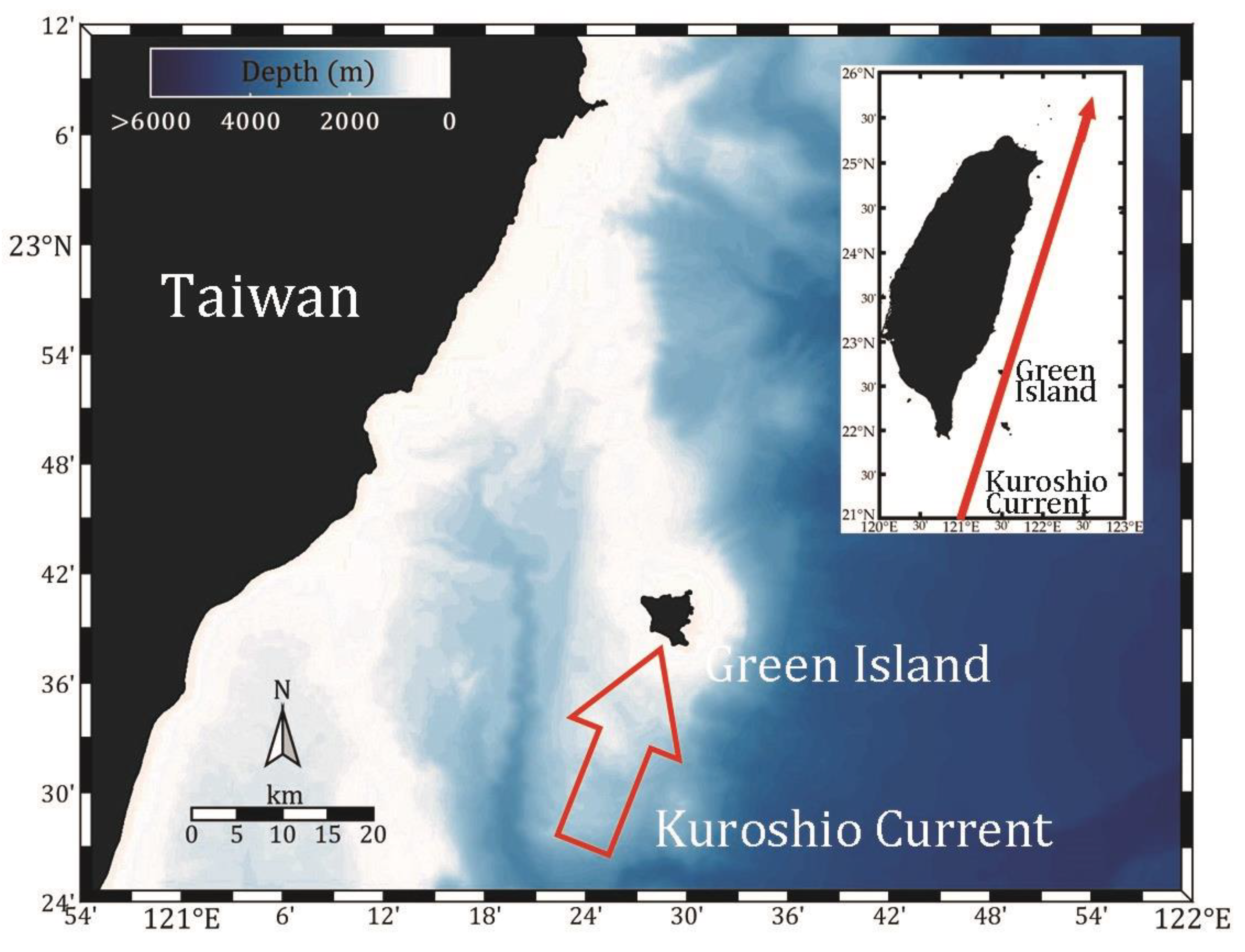
1.1. Background
1.2. Objectives
2. Materials and Methods
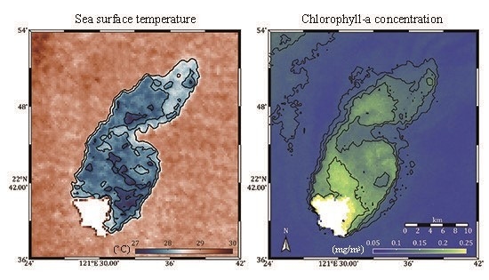
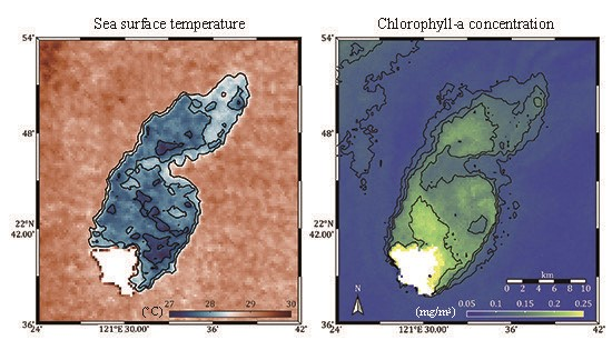
2.1. Sea Surface Temperature and Chlorophyll-a Concentration
2.2. Ocean Currents
2.3. Numerical Model
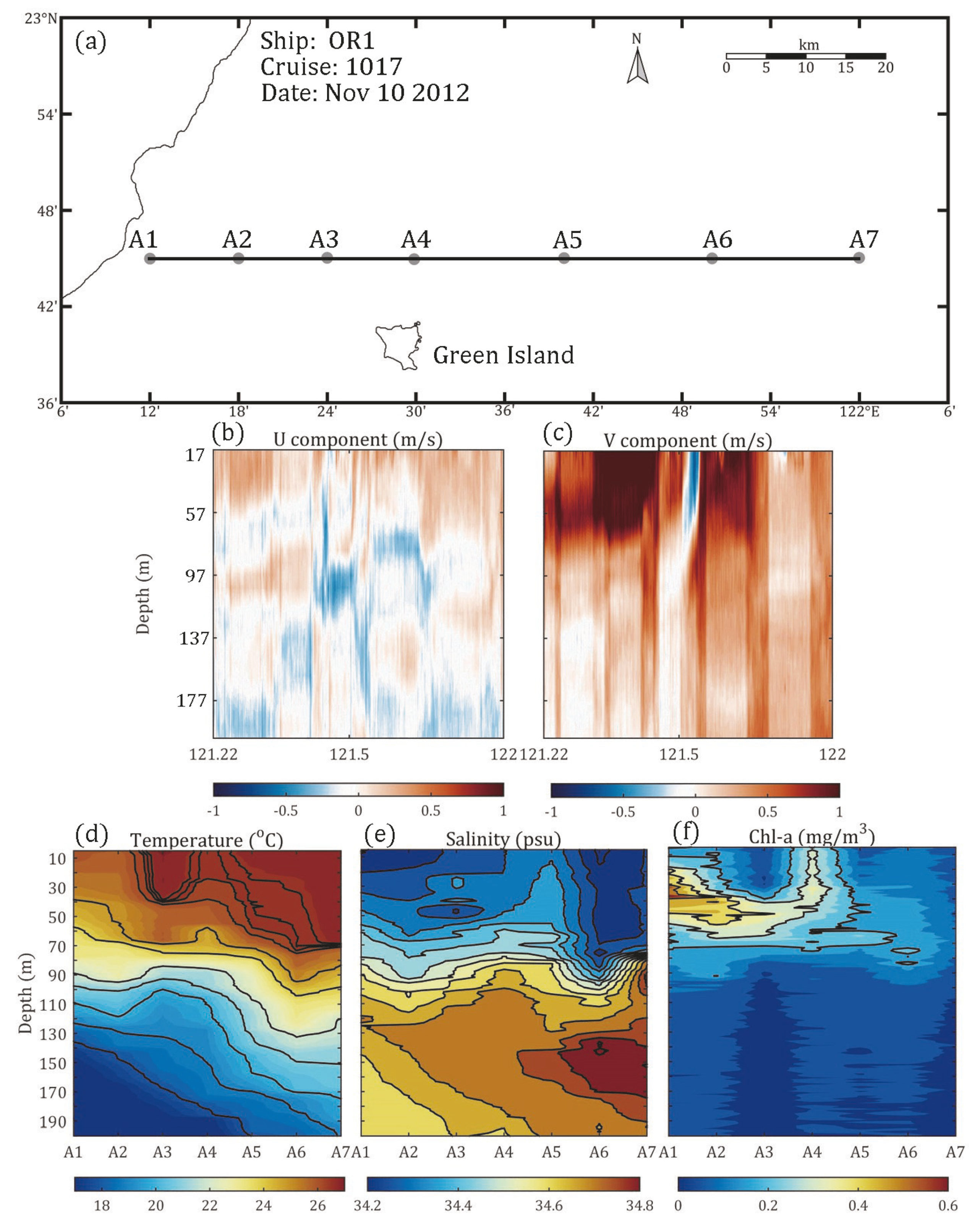
2.4. In-Situ Observation
3. Results
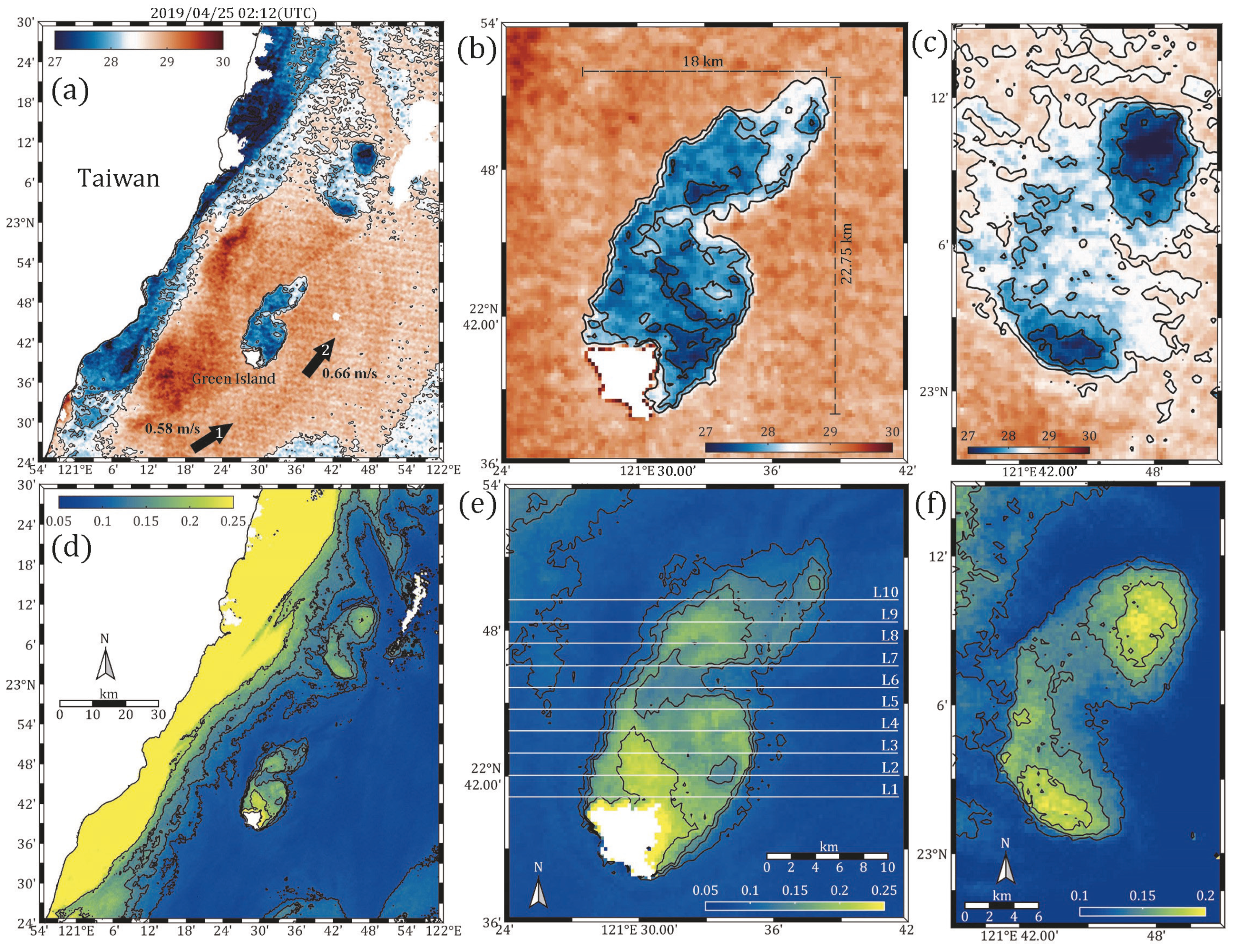
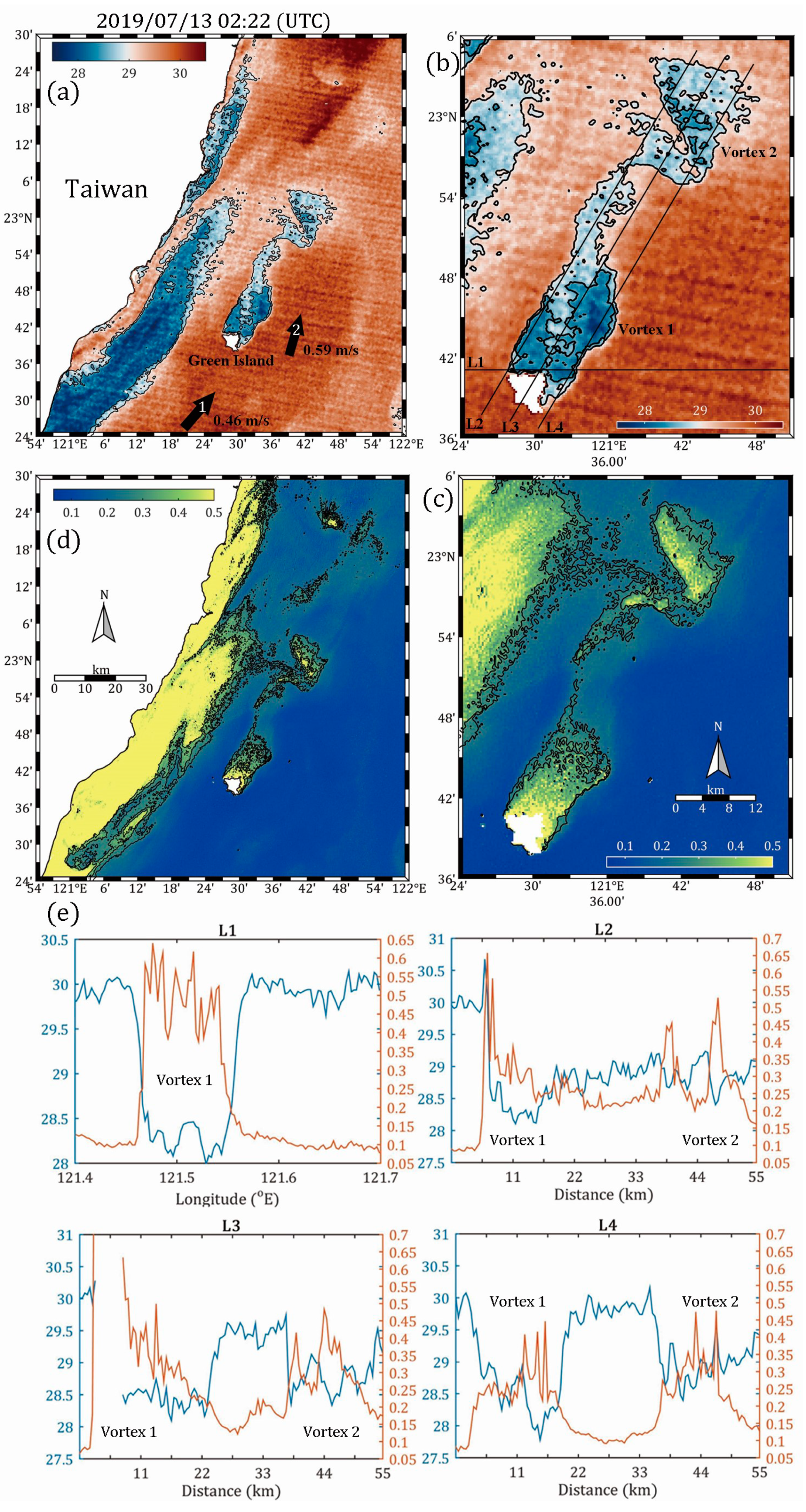
3.1. Field Experiment
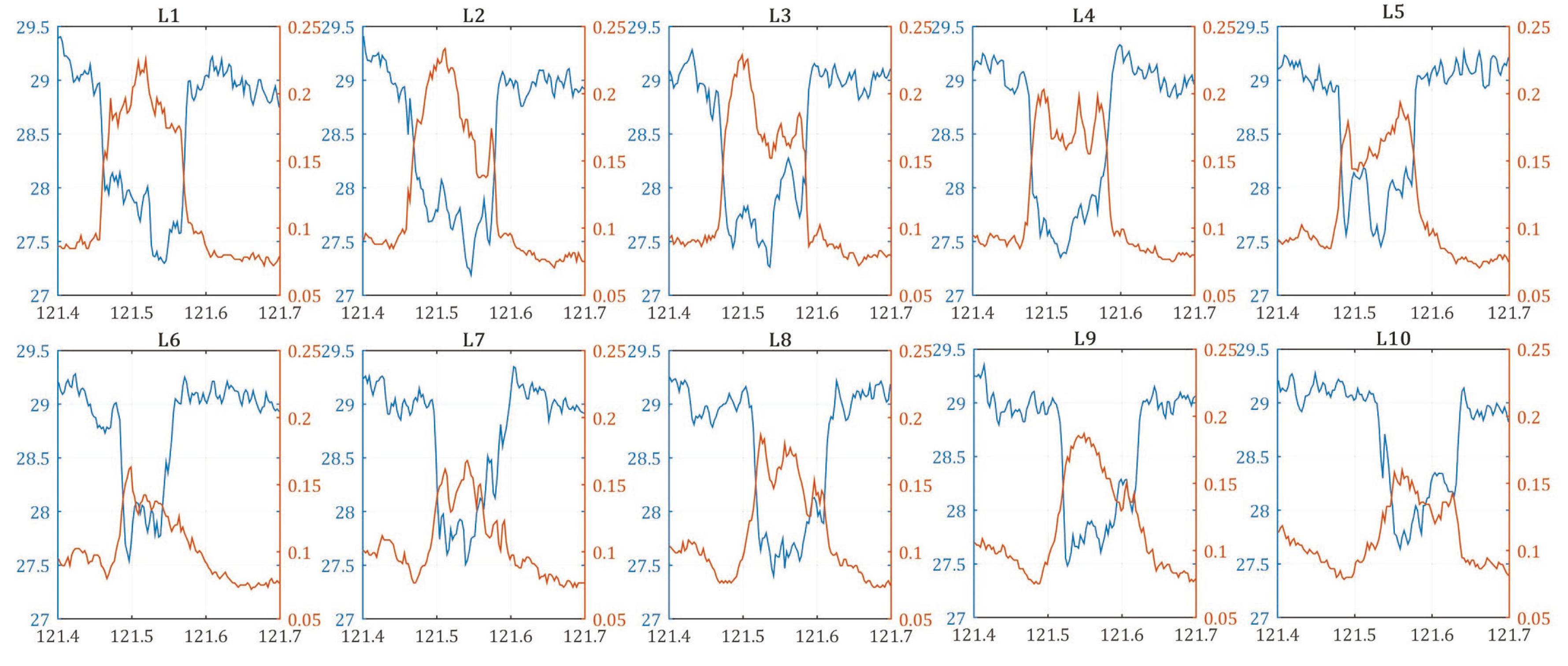
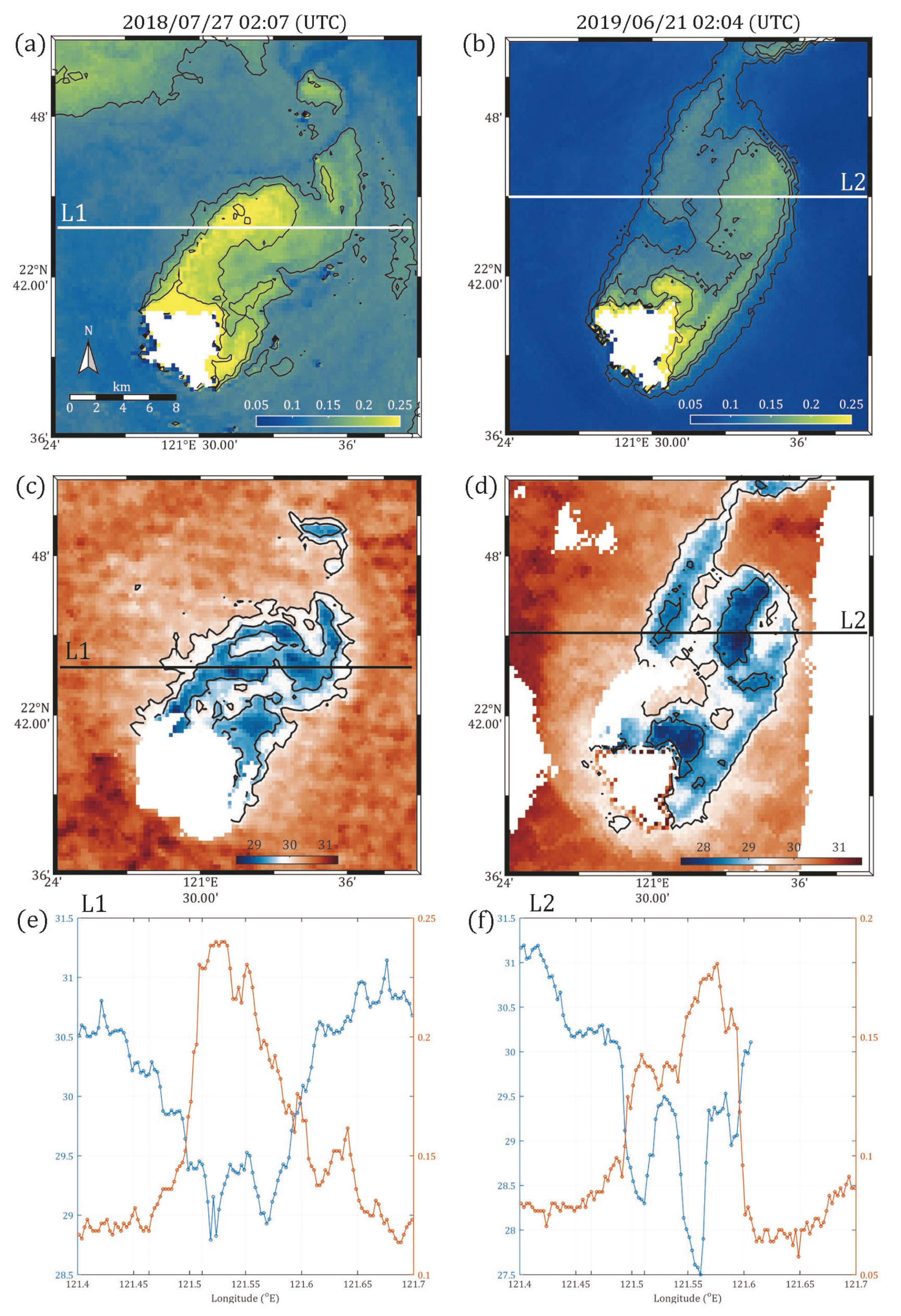
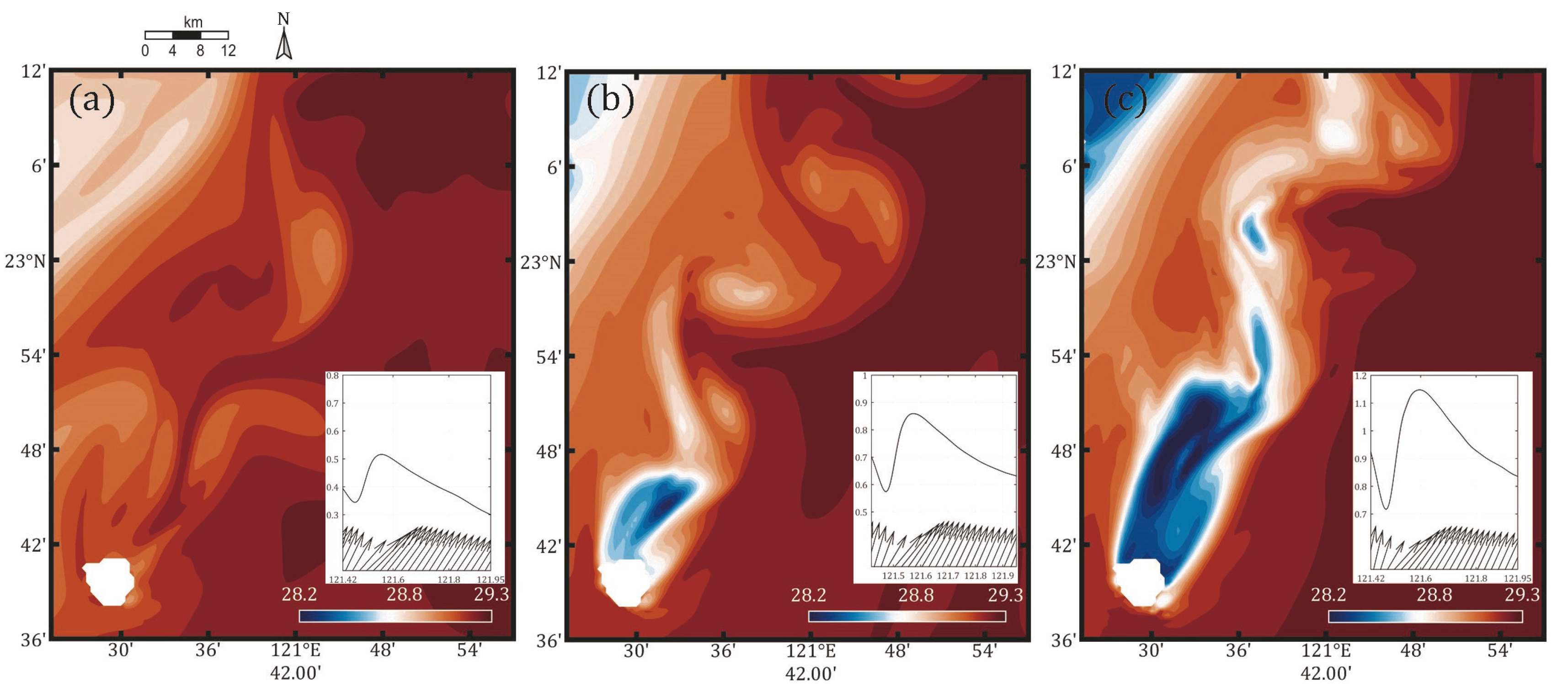
3.2. Spatial Structure of Island Wake
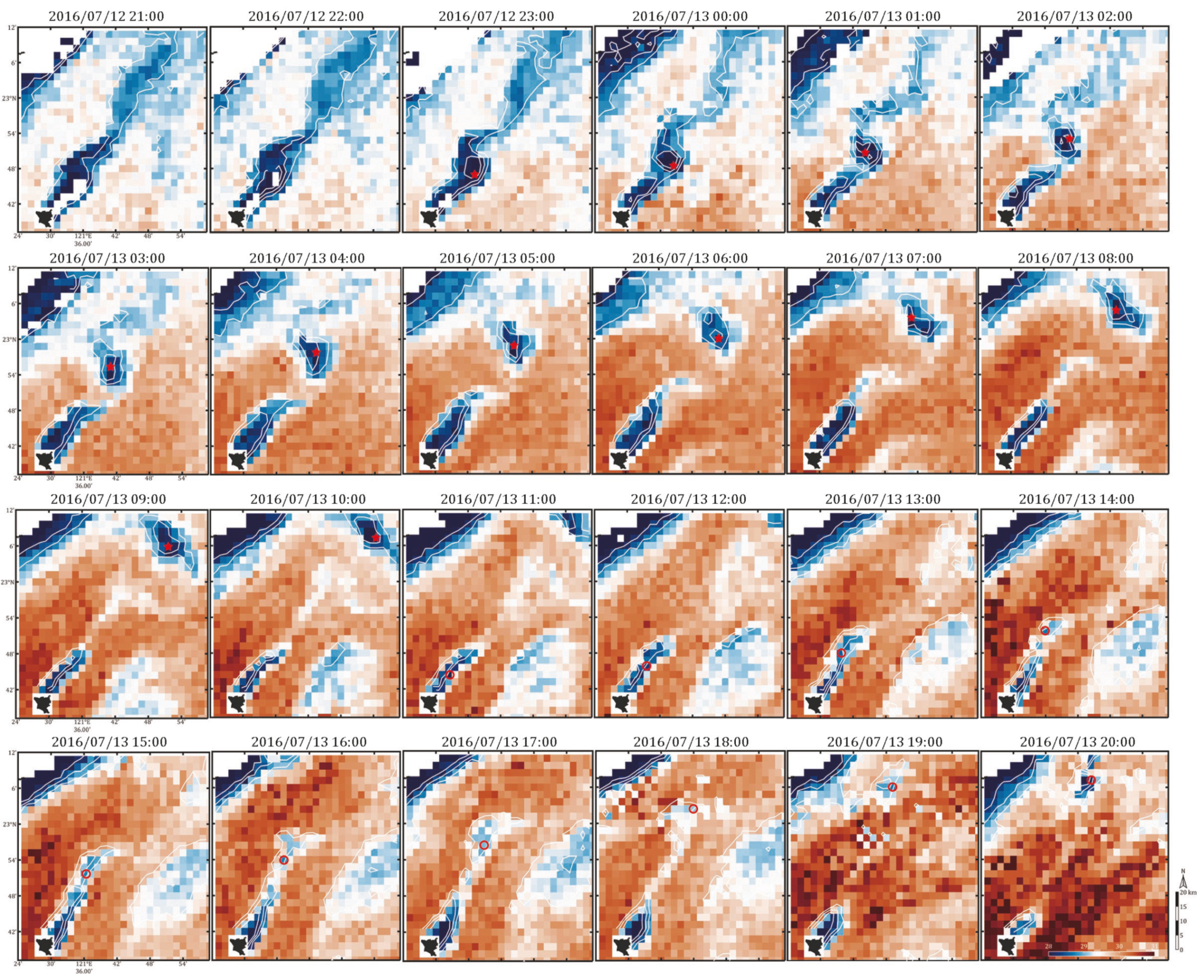
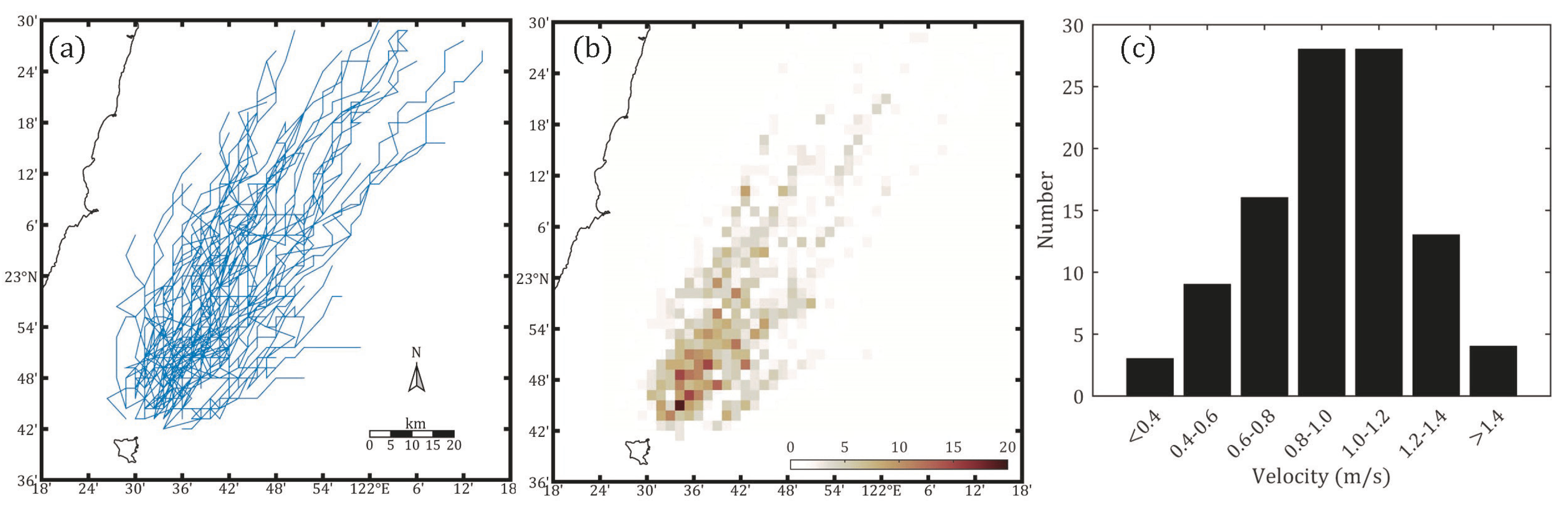
3.3. Temporal Variation and Vortex Trajectory
4. Discussion
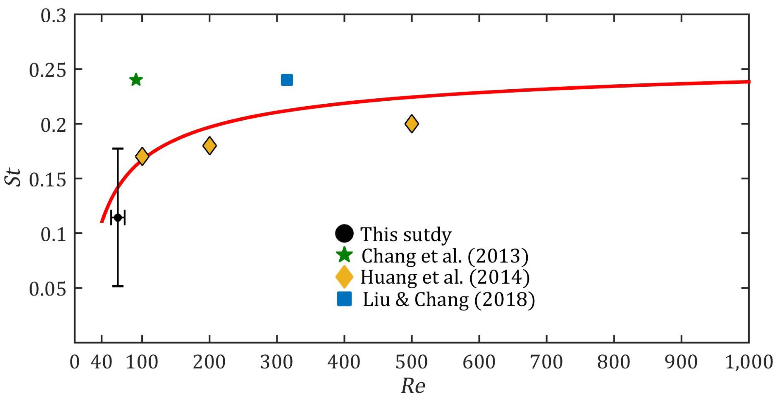
4.1. The Relationship Between Re and St
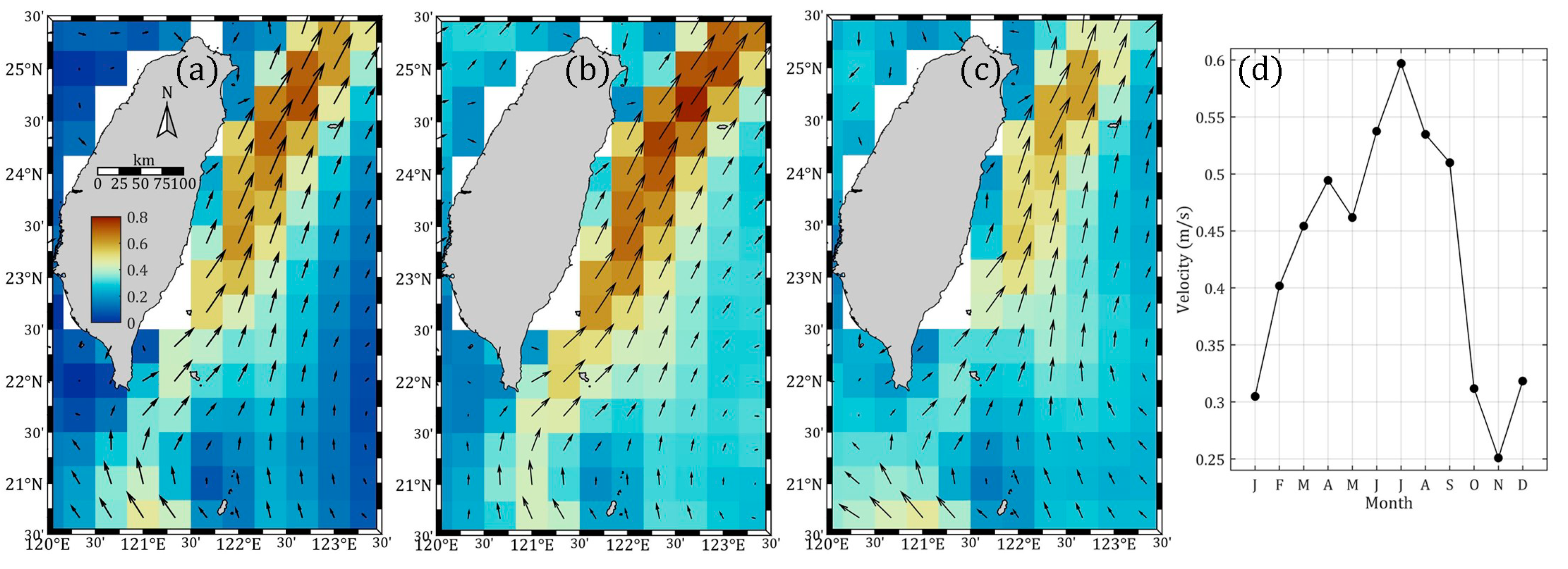
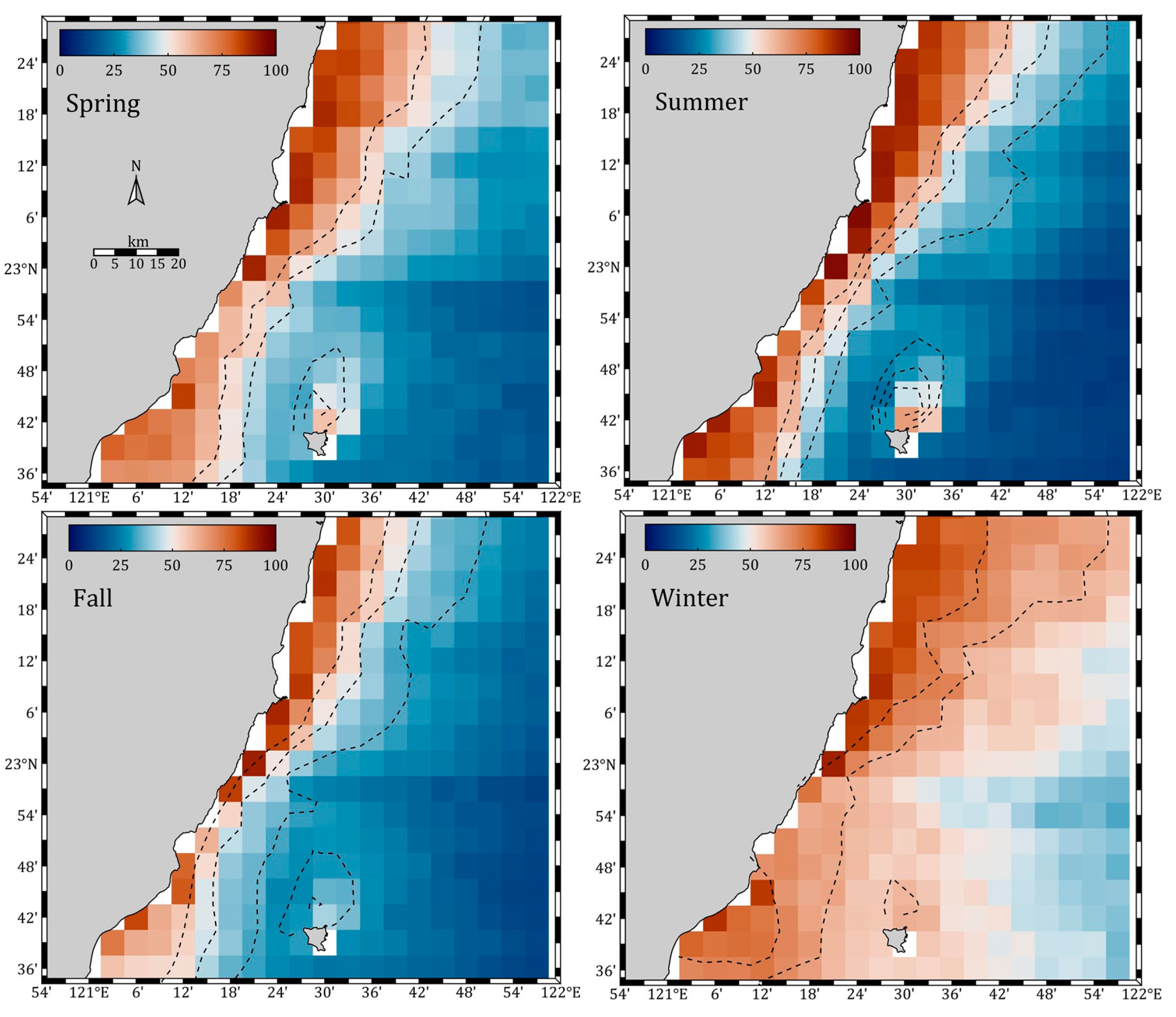
4.2. Seasonal Changes in and Chlorophyll-a Concentrations
4.3. Uncertainties, Errors, and Accuracies
5. Conclusions
Author Contributions
Funding
Acknowledgments
Conflicts of Interest
References
- Zeiden, K.L.; Rudnick, D.L.; MacKinnon, J.A. Glider observations of a mesoscale oceanic island wake. J. Phys. Oceanogr. 2019, 49, 2217–2235. [Google Scholar] [CrossRef]
- St. Laurent, L.; Ijichi, T.; Merrifield, S.T.; Shapiro, J.; Simmons, H.L. Turbulence and vorticity in the wake of Palau. Oceanography 2019, 32, 102–109. [Google Scholar] [CrossRef] [Green Version]
- Kodaira, T.; Waseda, T. Tidally generated island wakes and surface water cooling over Izu Ridge. Ocean Dyn. 2019, 69, 1373–1385. [Google Scholar] [CrossRef]
- Tanaka, T.; Hasegawa, D.; Yasuda, I.; Tsuji, H.; Fujio, S.; Goto, Y.; Nishioka, J. Enhanced vertical turbulent nitrate flux in the Kuroshio across the Izu Ridge. J. Oceanogr. 2019, 75, 195–203. [Google Scholar] [CrossRef]
- Chang, M.H.; Tang, T.Y.; Ho, C.R.; Chao, S.Y. Kuroshio-induced wake in the lee of Green Island off Taiwan. J. Geophys. Res. Ocean. 2013, 118, 1508–1519. [Google Scholar] [CrossRef]
- Huang, S.J.; Ho, C.R.; Lin, S.L.; Liang, S.J. Spatial-temporal scales of Green Island wake due to passing of the Kuroshio current. Int. J. Remote Sens. 2014, 35, 4484–4495. [Google Scholar] [CrossRef]
- Zheng, Z.W.; Zheng, Q. Variability of island-induced ocean vortex trains, in the Kuroshio region southeast of Taiwan Island. Cont. Shelf Res. 2014, 81, 1–6. [Google Scholar] [CrossRef]
- Hsu, P.C.; Chang, M.H.; Lin, C.C.; Huang, S.J.; Ho, C.R. Investigation of the island-induced ocean vortex train of the Kuroshio Current using satellite imagery. Remote Sens. Environ. 2017, 193, 54–64. [Google Scholar] [CrossRef]
- Hsu, P.C.; Cheng, K.H.; Jan, S.; Lee, H.J.; Ho, C.R. Vertical structure and surface patterns of Green Island wakes induced by the Kuroshio. Deep-Sea Res. Part I 2019, 143, 1–16. [Google Scholar] [CrossRef]
- Gove, J.M.; McManus, M.A.; Neuheimer, A.B.; Polovina, J.J.; Drazen, J.C.; Smith, C.R.; Merrifield, M.A.; Frienlander, A.M.; Ehses, J.S.; Young, C.W.; et al. Near-island biological hotspots in barren ocean basins. Nat. Commun. 2016, 7, 1–8. [Google Scholar] [CrossRef] [Green Version]
- Chen, T.C.; Ku, K.C.; Ying, T.C. A process-based collaborative model of marine tourism service system–The case of Green Island area, Taiwan. Ocean Coast. Manag. 2012, 64, 37–46. [Google Scholar] [CrossRef]
- Denis, V.; Soto, D.; De Palmas, S.; Lin, Y.T.; Benayahu, Y.; Huang, Y.; Liu, S.L.; Chen, J.W.; Chen, Q.; Sturaro, N.; et al. Mesophotic Coral Ecosystems. In Coral Reefs of the World; Loya, Y., Puglise, K., Bridge, T., Eds.; Springer: Cham, Switzerland, 2019; Volume 12, pp. 249–264. [Google Scholar] [CrossRef]
- Hsu, T.W.; Doong, D.J.; Hsieh, K.J.; Liang, S.J. Numerical study of monsoon effect on Green Island wake. J. Coast. Res. 2015, 31, 1141–1150. [Google Scholar] [CrossRef]
- Liu, C.L.; Chang, M.H. Numerical studies of submesoscale island wakes in the Kuroshio. J. Geophys. Res. Ocean. 2018, 123, 5669–5687. [Google Scholar] [CrossRef]
- Chang, M.H.; Jan, S.; Liu, C.L.; Cheng, Y.H.; Mensah, V. Observations of island wakes at high Rossby numbers: Evolution of submesoscale vortices and free shear layers. J. Phys. Oceanogr. 2019, 49, 2997–3016. [Google Scholar] [CrossRef]
- Zheng, Q.; Lin, H.; Meng, J.; Hu, X.; Song, Y.T.; Zhang, Y.; Li, C. Sub-mesoscale ocean vortex trains in the Luzon Strait. J. Geophys. Res. Ocean. 2008, 113. [Google Scholar] [CrossRef]
- Taniguchi, N.; Kida, S.; Sakuno, Y.; Mutsuda, H.; Syamsudin, F. Short-Term Variation of the Surface Flow Pattern South of Lombok Strait Observed from the Himawari-8 Sea Surface Temperature. Remote Sens.-Basel 2019, 11, 1491. [Google Scholar] [CrossRef] [Green Version]
- Liu, J.; Emery, W.J.; Wu, X.; Li, M.; Li, C.; Zhang, L. Computing Coastal Ocean Surface Currents from MODIS and VIIRS Satellite Imagery. Remote Sens. 2017, 9, 1083. [Google Scholar] [CrossRef] [Green Version]
- Hu, Z.; Qi, Y.; He, X.; Wang, Y.H.; Wang, D.P.; Cheng, X.; Liu, X.H.; Wang, T. Characterizing surface circulation in the Taiwan Strait during NE monsoon from Geostationary Ocean Color Imager. Remote Sens. Environ. 2019, 221, 687–694. [Google Scholar] [CrossRef]
- Ditri, A.L.; Minnett, P.J.; Liu, Y.; Kilpatrick, K.; Kumar, A. The Accuracies of Himawari-8 and MTSAT-2 sea-surface temperatures in the tropical western Pacific Ocean. Remote Sens. 2018, 10, 212. [Google Scholar] [CrossRef] [Green Version]
- ESR. OSCAR Third Degree Resolution Ocean Surface Currents; Ver. 1; PO.DAAC: Pasadena, CA, USA, 2009. [Google Scholar] [CrossRef]
- Bonjean, F.; Lagerloef, G.S.E. Diagnostic model and analysis of the surface currents in the tropical Pacific Ocean. J. Phys. Oceanogr. 2002, 32, 2938–2954. [Google Scholar] [CrossRef]
- Johnson, E.S.; Bonjean, F.; Lagerloef, G.S.; Gunn, J.T.; Mitchum, G.T. Validation and error analysis of OSCAR sea surface currents. J. Atmos. Ocean. Technol. 2007, 24, 688–701. [Google Scholar] [CrossRef]
- Marshall, J.; Adcroft, A.; Hill, C.; Perelman, L.; Heisey, C. A finite-volume, incompressible Navier Stokes model for studies of the ocean on parallel computers. J. Geophys. Res. Ocean. 1997, 102, 5753–5766. [Google Scholar] [CrossRef] [Green Version]
- Orlanski, I. A simple boundary condition for unbounded hyperbolic flows. J. Comput. Phys. 1976, 21, 251–269. [Google Scholar] [CrossRef]
- Klymak, J.M.; Legg, S.M. A simple mixing scheme for models that resolve breaking internal waves. Ocean. Model. 2010, 33, 224–234. [Google Scholar] [CrossRef]
- Williamson, C.H.K.; Brown, G.L. A series in 1/√ Re to represent the Strouhal–Reynolds number relationship of the cylinder wake. J. Fluids Struct. 1998, 12, 1073–1085. [Google Scholar] [CrossRef]
- Apel, J.R. Principles of Ocean Physics; Academic Press: London, UK, 1987. [Google Scholar]
- Hsu, P.C.; Lin, C.C.; Huang, S.J.; Ho, C.R. Effects of cold eddy on Kuroshio meander and its surface properties, east of Taiwan. IEEE J.-STARS 2016, 9, 5055–5063. [Google Scholar] [CrossRef]
- Kurihara, Y.; Murakami, H.; Kachi, M. Sea surface temperature from the new Japanese geostationary meteorological Himawari-8 satellite. Geophys. Res. Lett. 2016, 43, 1234–1240. [Google Scholar] [CrossRef] [Green Version]


| L (m) | Reference | ||||
|---|---|---|---|---|---|
| 7000 | 1.3 | 100 | 91 | 0.24 | [5] |
| 5000 | 1 | 50 | 100 200 500 | 0.17 0.18 0.20 | [6] |
| 7000 | 0.675 | 15 | 315 | 0.24 | [14] |
| 5500 | 100 | This study |
| Average | Maximum | Minimum | |
|---|---|---|---|
| Spring | 0.47 ± 0.10 | 0.82 | 0.27 |
| Summer | 0.56 ± 0.13 | 0.94 | 0.28 |
| Fall | 0.36 ± 0.18 | 0.84 | 0.02 |
| Winter | 0.34 ± 0.13 | 0.63 | 0.02 |
© 2020 by the authors. Licensee MDPI, Basel, Switzerland. This article is an open access article distributed under the terms and conditions of the Creative Commons Attribution (CC BY) license (http://creativecommons.org/licenses/by/4.0/).
Share and Cite
Hsu, P.-C.; Ho, C.-Y.; Lee, H.-J.; Lu, C.-Y.; Ho, C.-R. Temporal Variation and Spatial Structure of the Kuroshio-Induced Submesoscale Island Vortices Observed from GCOM-C and Himawari-8 Data. Remote Sens. 2020, 12, 883. https://0-doi-org.brum.beds.ac.uk/10.3390/rs12050883
Hsu P-C, Ho C-Y, Lee H-J, Lu C-Y, Ho C-R. Temporal Variation and Spatial Structure of the Kuroshio-Induced Submesoscale Island Vortices Observed from GCOM-C and Himawari-8 Data. Remote Sensing. 2020; 12(5):883. https://0-doi-org.brum.beds.ac.uk/10.3390/rs12050883
Chicago/Turabian StyleHsu, Po-Chun, Chia-Ying Ho, Hung-Jen Lee, Ching-Yuan Lu, and Chung-Ru Ho. 2020. "Temporal Variation and Spatial Structure of the Kuroshio-Induced Submesoscale Island Vortices Observed from GCOM-C and Himawari-8 Data" Remote Sensing 12, no. 5: 883. https://0-doi-org.brum.beds.ac.uk/10.3390/rs12050883