Assessment of Workflow Feature Selection on Forest LAI Prediction with Sentinel-2A MSI, Landsat 7 ETM+ and Landsat 8 OLI

 ,
,  , , , , and
Abstract
:
1. Introduction
2. Data
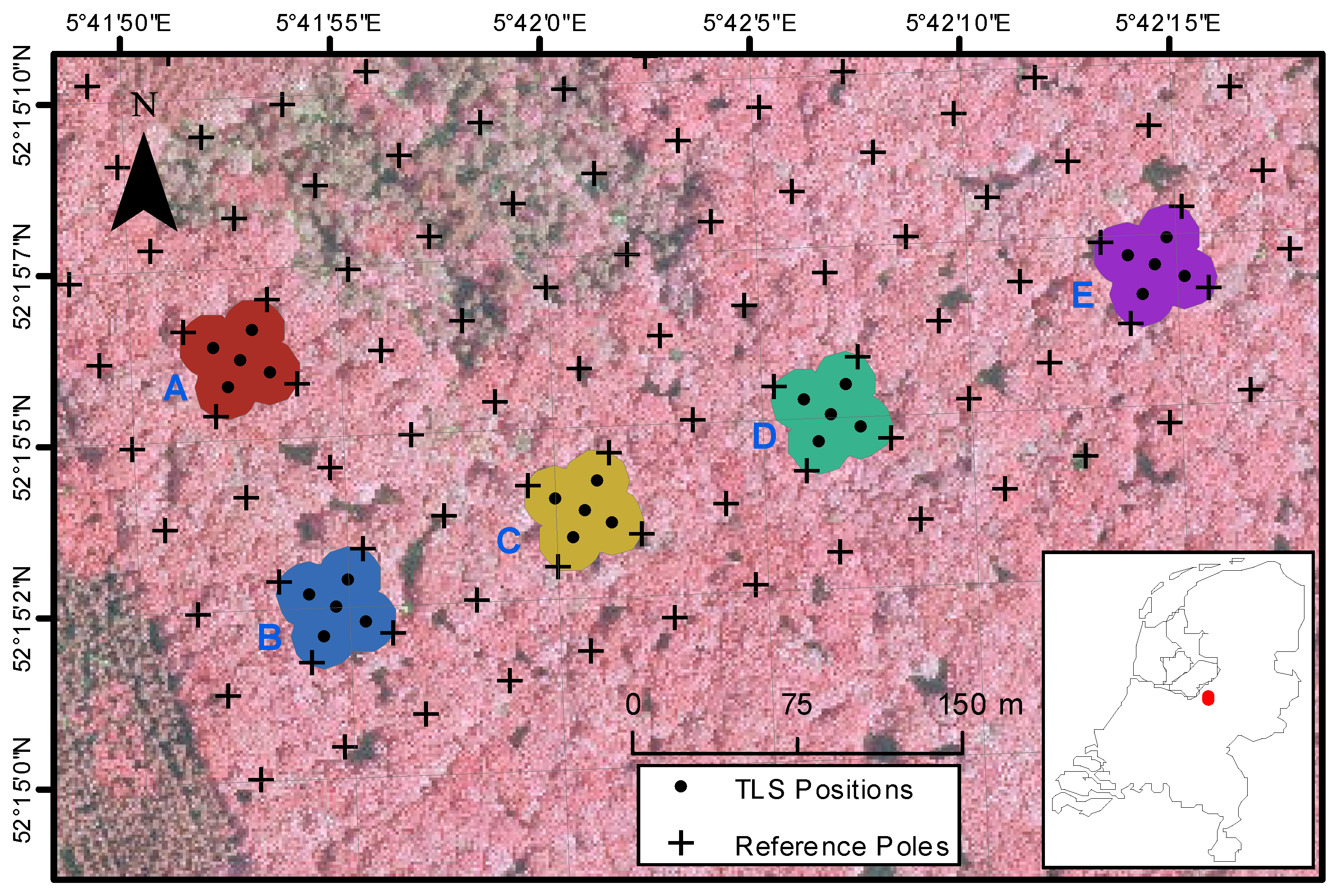
2.1. Study Site
2.2. Field Data
2.2.1. Terrestrial Laser Scanning (TLS) Data
2.2.2. Littertrap Data
2.2.3. Leaf Sampling Data
2.3. Satellite Data
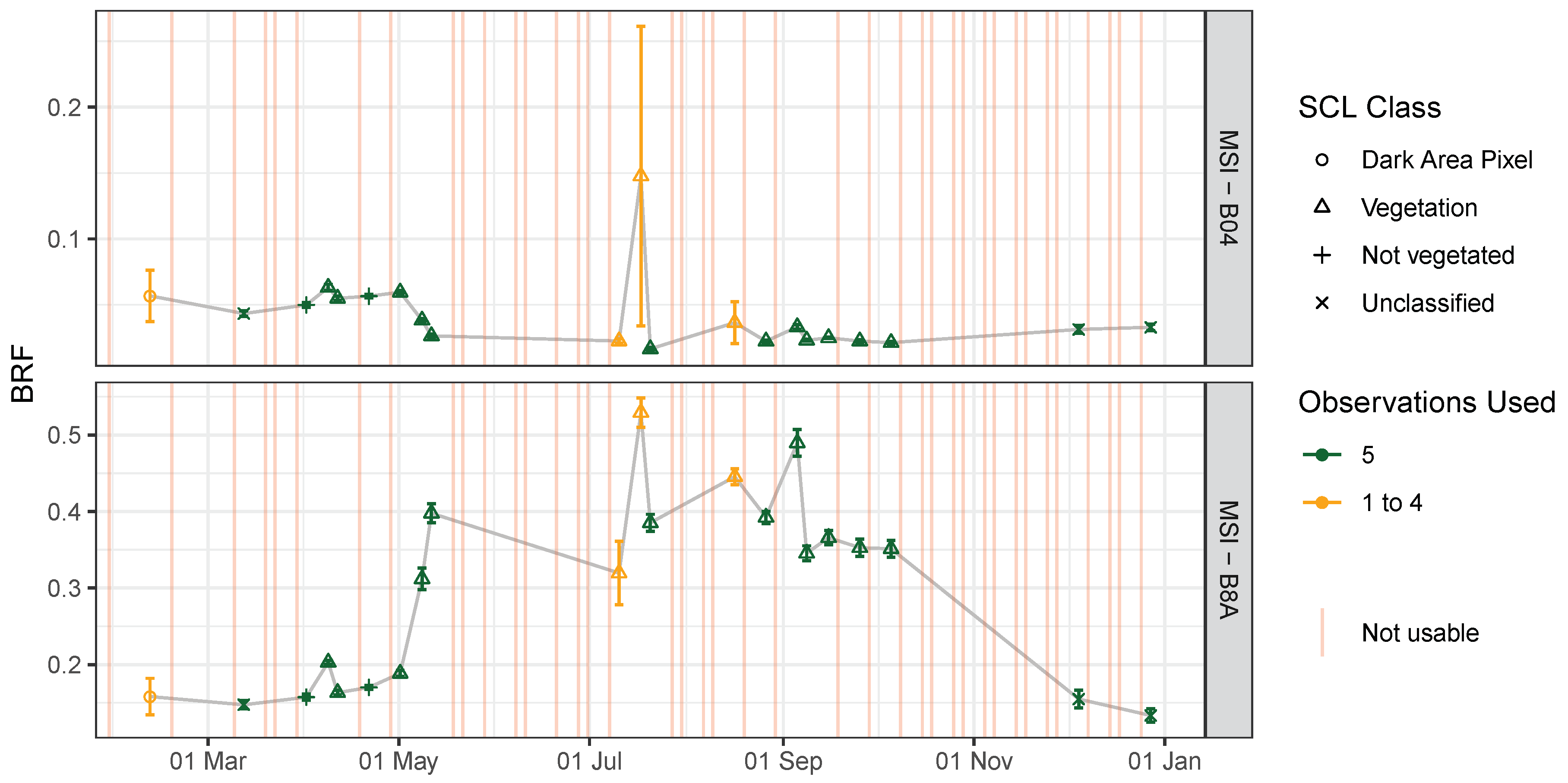
2.3.1. Sentinel-2A MSI
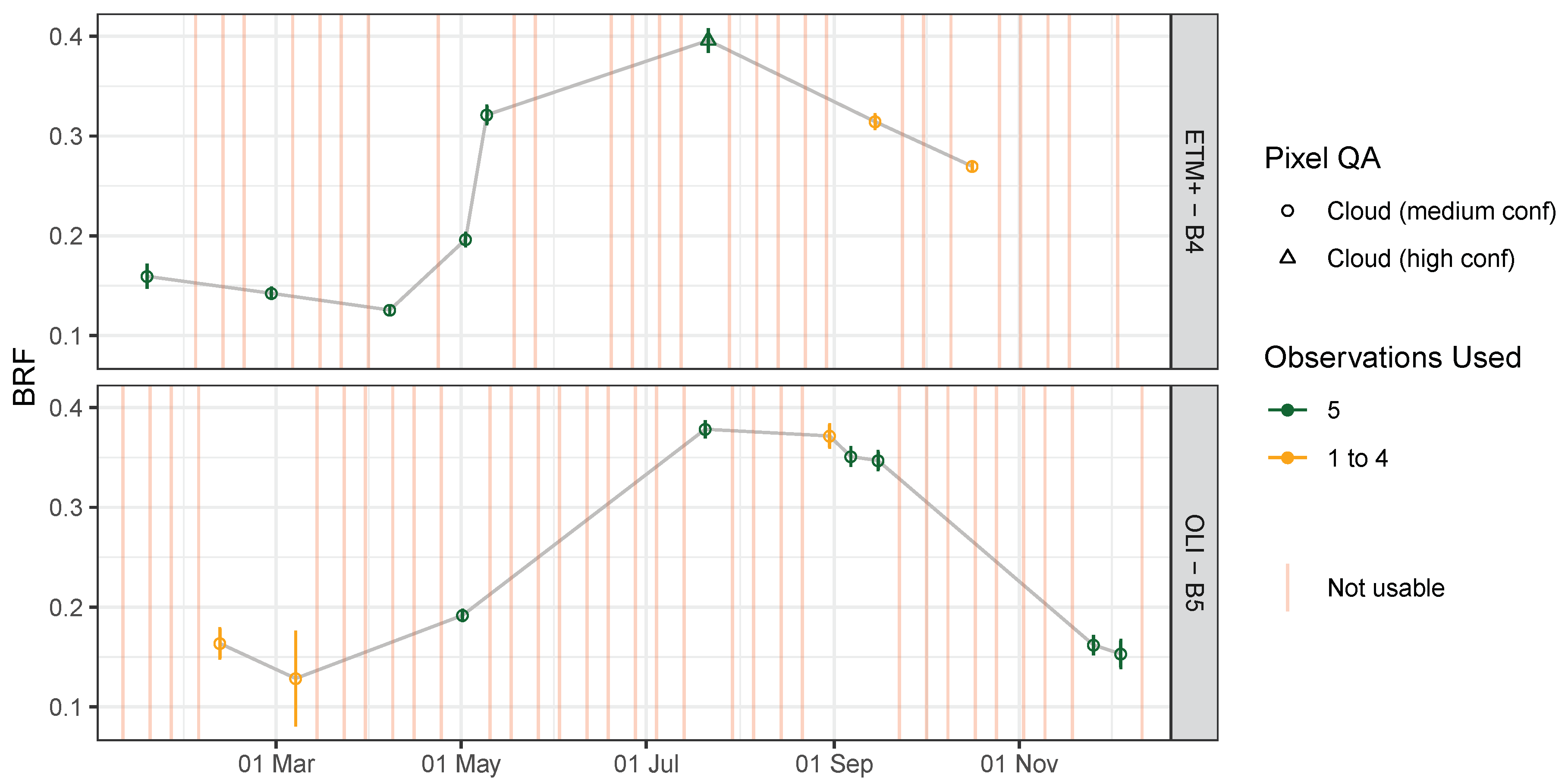
2.3.2. Landsat ETM+ and OLI
3. Methods
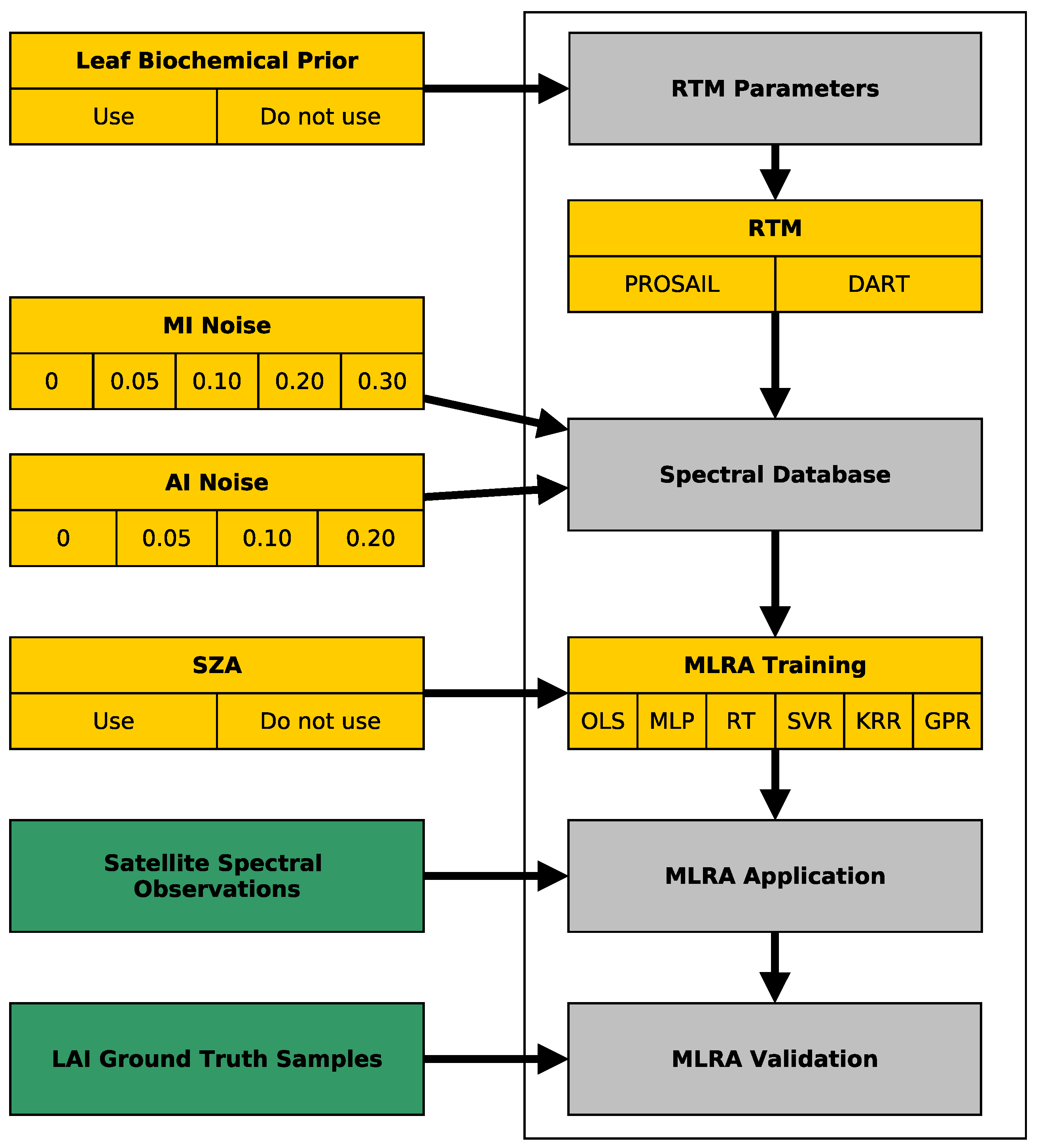
- A vegetation RTM is run in forward mode to create a database of training samples, i.e., biophysical parameters serve as input for the RTM to predict spectral BRFs. The parameter values are altered to cover multiple canopy conditions.
- Gaussian noise is added to the spectra to prevent the MLRA from over-fitting and simulate observation noise.
- Multiple MLRAs are trained on the database to learn the inverse mapping, i.e., from spectral bands to biophysical parameter. Model hyperparameter tuning is performed on a part of the generated database, while the rest is used for testing the trained model.
- The MLRAs are applied to the observed spectra to predict the biophysical parameter of interest. MLRAs performance is compared.
- Biochemical Prior: Using leaf biochemical parameters inferred from field spectroscopy observations to restrict the RTM input parameter space (label: prior knowledge) versus using a free range (label: free) (two alternatives).
- RTM: Two underlying, structurally contrasting RTMs were tested: turbid medium PROSAIL (SAIL 4 coupled with PROSPECT 5) and structurally-explicit Discrete Anisotropic Radiative Transfer (DART) (with PROSPECT 5) (two alternatives).
- Noise scenario: Using multiple noise levels for two types of noise (four and five alternatives).
- SZA: Using the SZA as an additional learning feature (label: SZA) or not (label: no SZA) (two alternatives).
- MLRA: Using multiple MLRAs: Ordinary Least Squares (OLS), Multi-Layer Perceptron (MLP), Regression Tree (RT), Support Vector Regression (SVR), Kernel Ridge Regression (KRR), GPR (six alternatives).
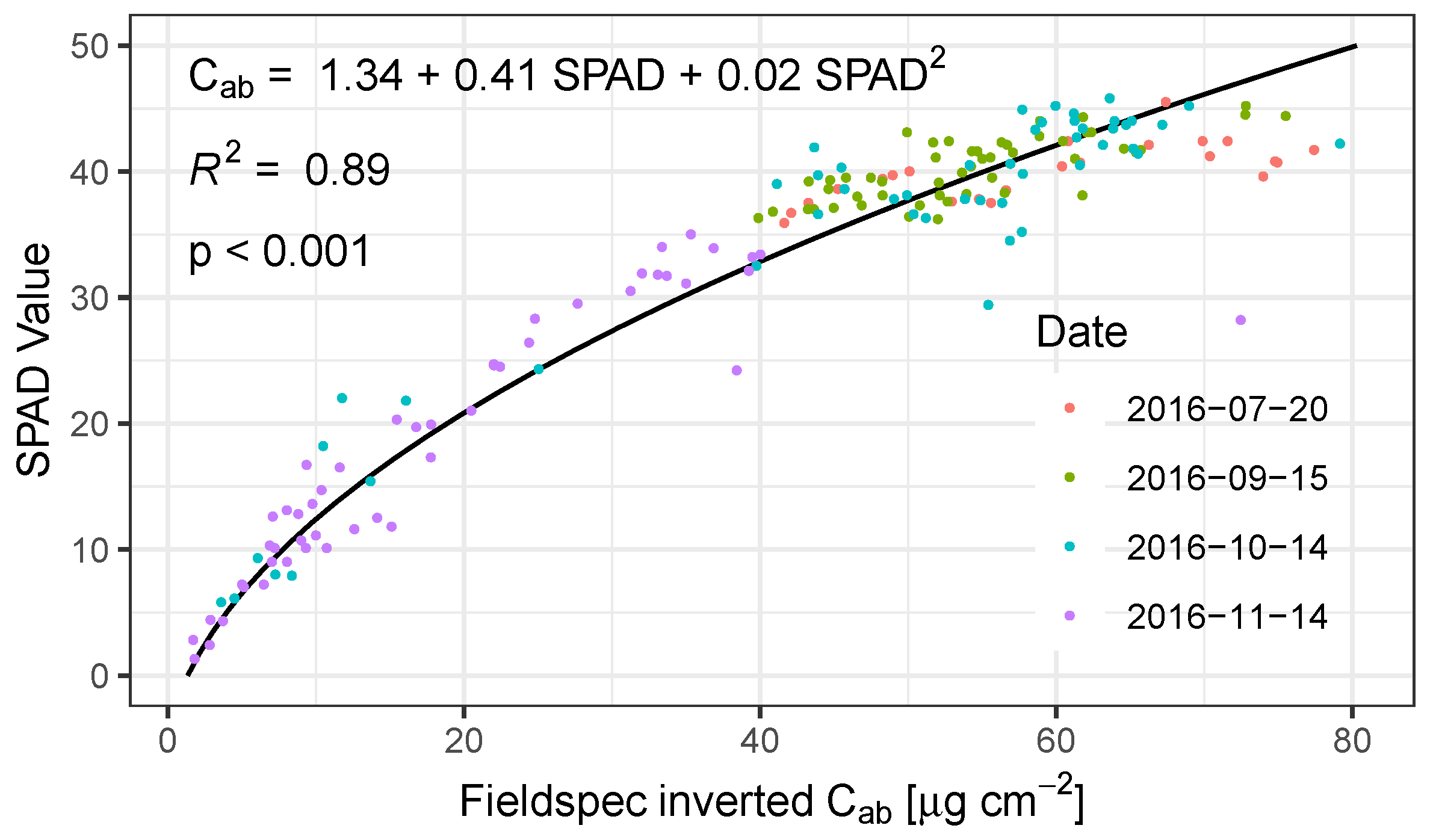
3.1. Leaf Biochemical Parameter Estimation
3.2. RTMs and Training Database Generation
3.3. RTM Sensitivity Analysis
3.4. Noise Scenarios
3.5. Solar Zenith Angle
3.6. Machine Learning Regression Algorithms
3.7. Ensemble Analysis and Validation
4. Results and Discussion
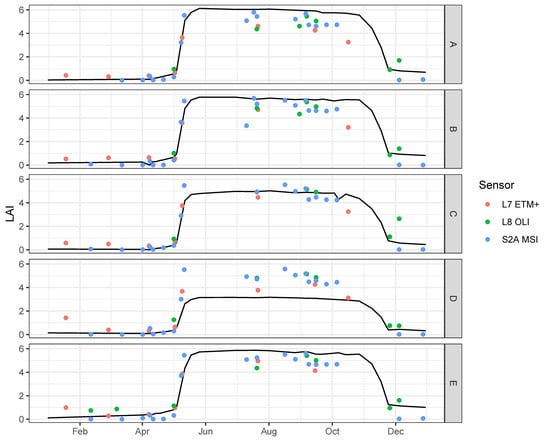
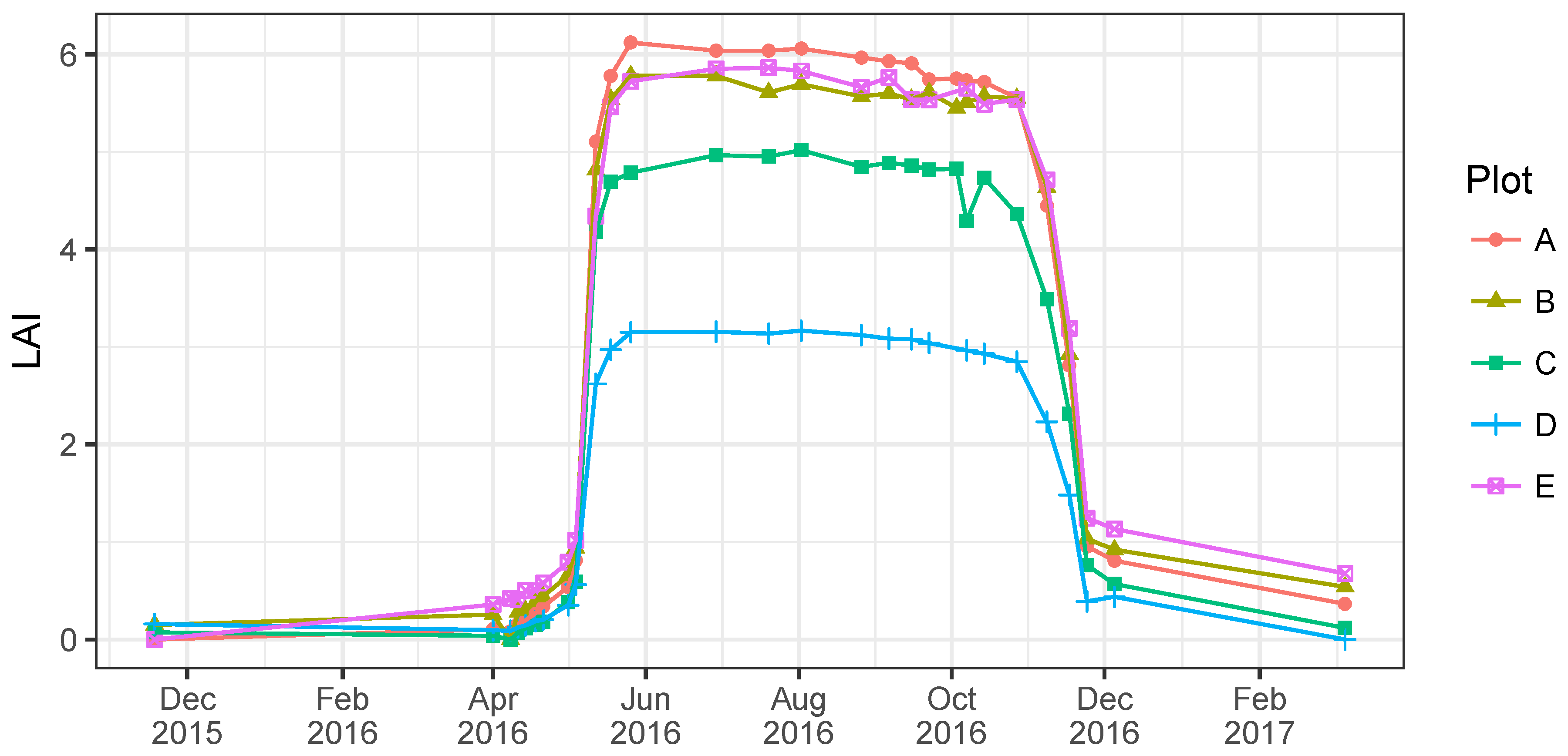
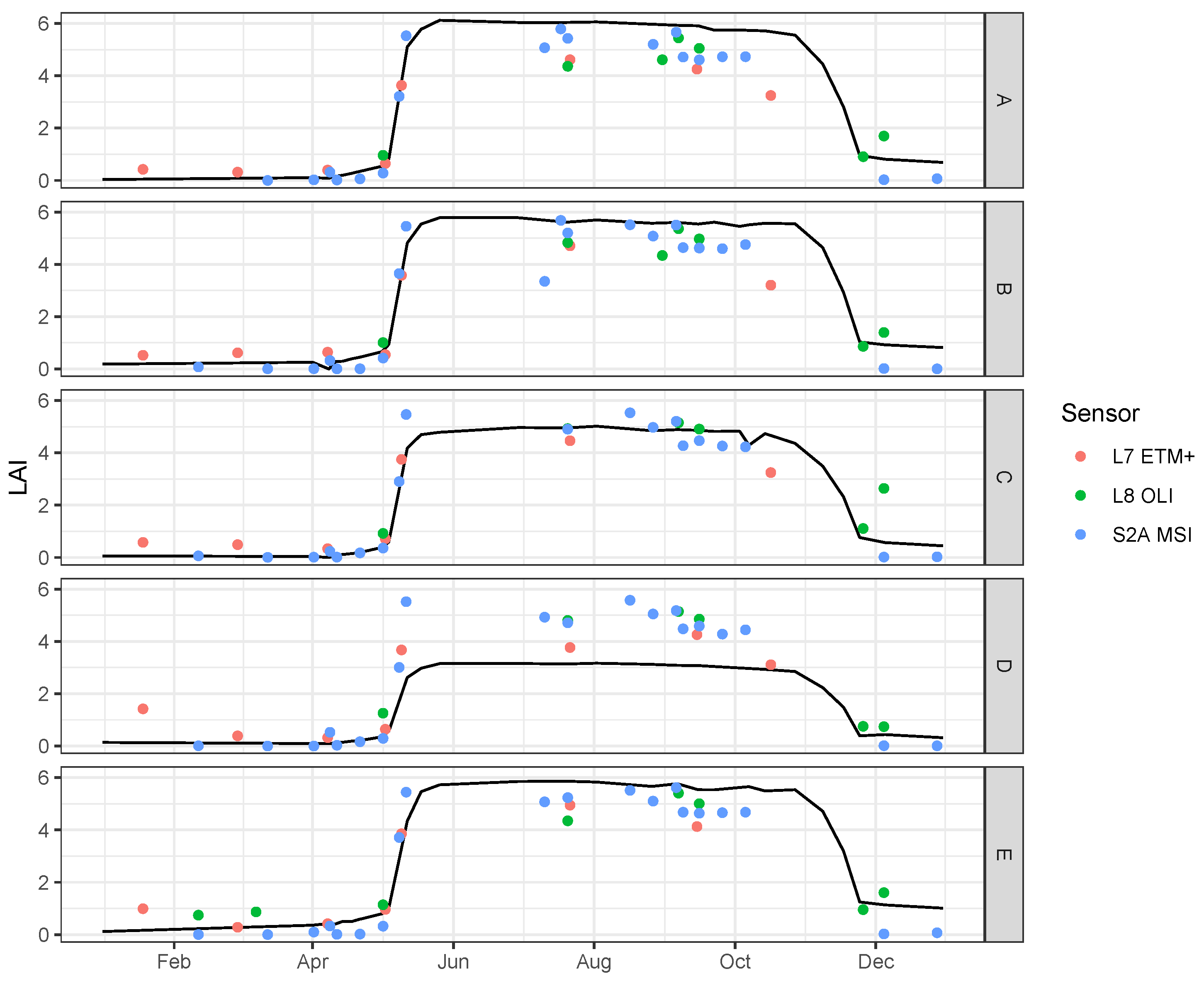
4.1. Validation Time Series
4.2. Leaf Biochemical Parameters’ Retrieval
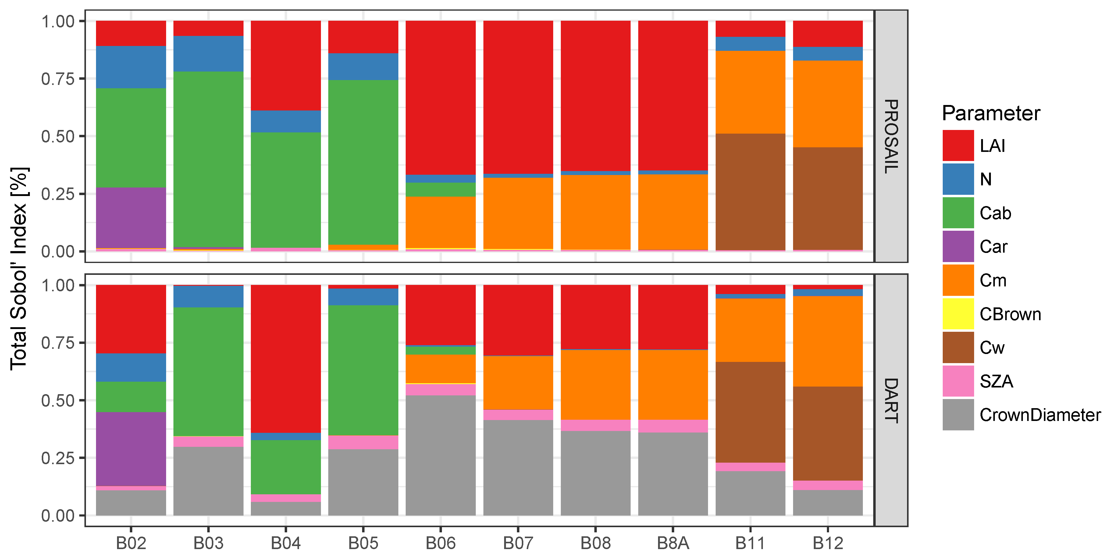
4.3. RTM Sensitivity
4.4. Impact of Training Scheme Features on Prediction Performance
4.4.1. Leaf Biochemical Prior
4.4.2. RTM Choice
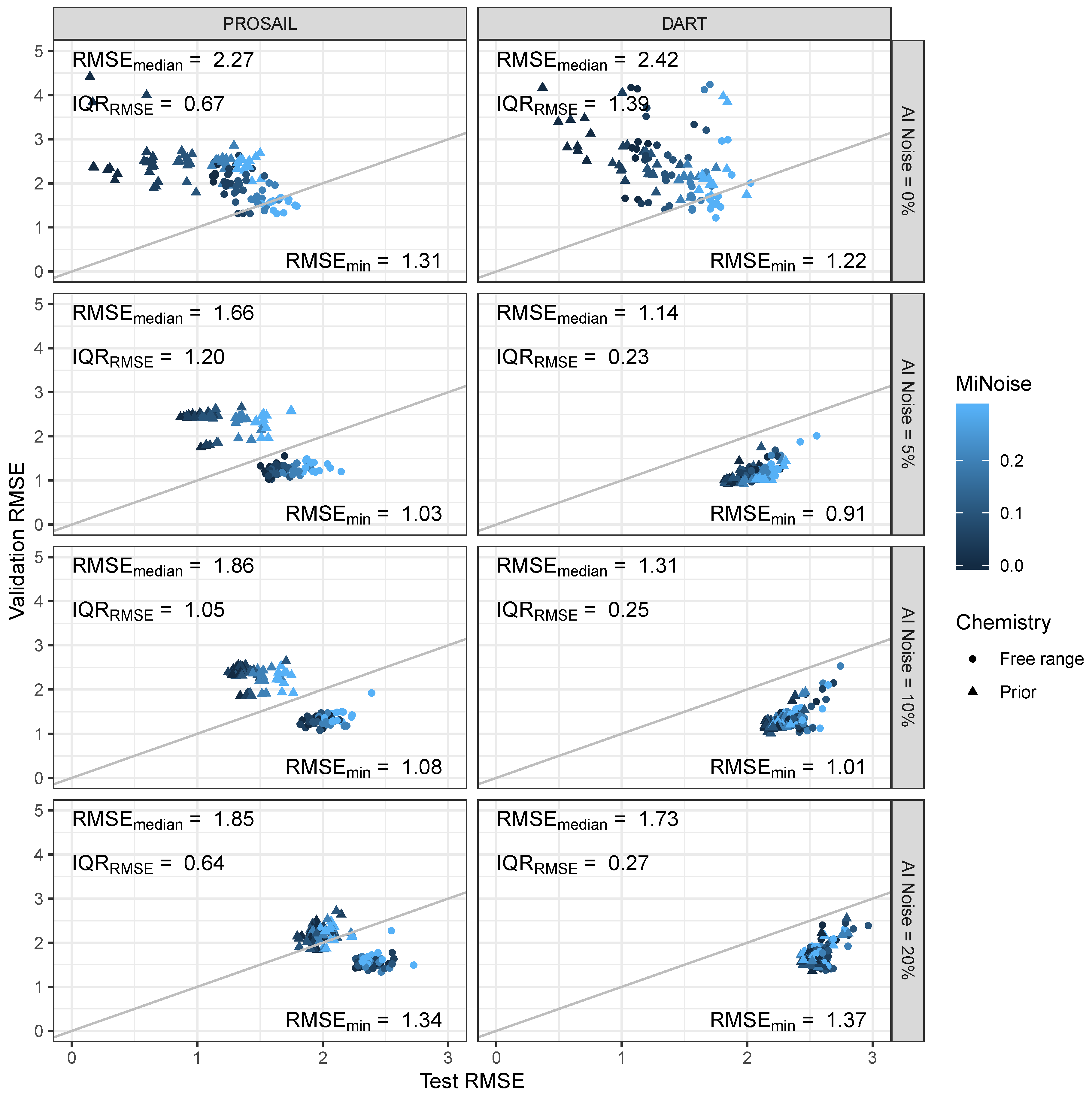
4.4.3. Noise Scenarios
4.4.4. SZA
4.4.5. MLRA
4.5. Best Performing Feature Combination
5. Conclusions
Author Contributions
Funding
Acknowledgments
Conflicts of Interest
Appendix A


| TLS | Landsat 7 | Landsat 8 | Sentinel-2A |
|---|---|---|---|
| 2015-11-18 | 2016-01-18 | 2016-02-11 | 2016-02-11 |
| 2016-04-01 | 2016-02-28 | 2016-03-07 | 2016-03-12 |
| 2016-04-08 | 2016-04-07 | 2016-05-01 | 2016-04-01 |
| 2016-04-11 | 2016-05-02 | 2016-07-20 | 2016-04-08 |
| 2016-04-14 | 2016-05-09 | 2016-08-30 | 2016-04-11 |
| 2016-04-18 | 2016-07-21 | 2016-09-06 | 2016-04-21 |
| 2016-04-21 | 2016-09-14 | 2016-09-15 | 2016-05-01 |
| 2016-05-01 | 2016-10-16 | 2016-11-25 | 2016-05-08 |
| 2016-05-04 | 2016-12-04 | 2016-05-11 | |
| 2016-05-12 | 2016-07-10 | ||
| 2016-05-18 | 2016-07-17 | ||
| 2016-05-26 | 2016-07-20 | ||
| 2016-06-29 | 2016-08-16 | ||
| 2016-07-20 | 2016-08-26 | ||
| 2016-08-02 | 2016-09-05 | ||
| 2016-08-26 | 2016-09-08 | ||
| 2016-09-06 | 2016-09-15 | ||
| 2016-09-15 | 2016-09-25 | ||
| 2016-09-22 | 2016-10-05 | ||
| 2016-10-03 | 2016-12-04 | ||
| 2016-10-07 | 2016-12-27 | ||
| 2016-10-14 | |||
| 2016-10-27 | |||
| 2016-11-08 | |||
| 2016-11-17 | |||
| 2016-11-24 | |||
| 2016-12-05 | |||
| 2017-03-07 |
References
- Beer, C.; Reichstein, M.; Tomelleri, E.; Ciais, P.; Jung, M.; Carvalhais, N.; Rödenbeck, C.; Arain, M.A.; Baldocchi, D.; Bonan, G.B.; et al. Terrestrial gross carbon dioxide uptake: Global distribution and covariation with climate. Science 2010, 329, 834–838. [Google Scholar] [CrossRef] [PubMed] [Green Version]
- Chen, J.; Black, T.A. Defining leaf area index for non-flat leaves. Plant Cell Environ. 1992, 15, 421–429. [Google Scholar] [CrossRef]
- Malenovský, Z.; Rott, H.; Cihlar, J.; Schaepman, M.E.; García-Santos, G.; Fernandes, R.; Berger, M. Sentinels for science: Potential of Sentinel-1, -2, and -3 missions for scientific observations of ocean, cryosphere, and land. Remote Sens. Environ. 2012, 120, 91–101. [Google Scholar] [CrossRef]
- Morisette, J.T.; Baret, F.; Privette, J.L.; Myneni, R.B.; Nickeson, J.E.; Garrigues, S.; Shabanov, N.V.; Weiss, M.; Fernandes, R.A.; Leblanc, S.G.; et al. Validation of global moderate-resolution LAI products: A framework proposed within the CEOS land product validation subgroup. IEEE Trans. Geosci. Remote Sens. 2006, 44, 1804–1814. [Google Scholar] [CrossRef] [Green Version]
- Jacquemoud, S.; Verhoef, W.; Baret, F.; Bacour, C.; Zarco-Tejada, P.J.; Asner, G.P.; François, C.; Ustin, S.L. PROSPECT + SAIL models: A review of use for vegetation characterization. Remote Sens. Environ. 2009, 113, S56–S66. [Google Scholar] [CrossRef]
- Roy, D.P.; Wulder, M.A.; Loveland, T.R.; Woodcock, C.E.; Allen, R.G.; Anderson, M.C.; Helder, D.; Irons, J.R.; Johnson, D.M.; Kennedy, R.; et al. Landsat-8: Science and product vision for terrestrial global change research. Remote Sens. Environ. 2014, 145, 154–172. [Google Scholar] [CrossRef] [Green Version]
- Houborg, R.; McCabe, M.; Cescatti, A.; Gao, F.; Schull, M.; Gitelson, A. Joint leaf chlorophyll content and leaf area index retrieval from Landsat data using a regularized model inversion system (REGFLEC). Remote Sens. Environ. 2015, 159, 203–221. [Google Scholar] [CrossRef] [Green Version]
- Li, W.; Weiss, M.; Waldner, F.; Defourny, P.; Demarez, V.; Morin, D.; Hagolle, O.; Baret, F. A Generic Algorithm to Estimate LAI, FAPAR and FCOVER Variables from SPOT4_HRVIR and Landsat Sensors: Evaluation of the Consistency and Comparison with Ground Measurements. Remote Sens. 2015, 7, 15494–15516. [Google Scholar] [CrossRef] [Green Version]
- Yin, G.; Verger, A.; Qu, Y.; Zhao, W.; Xu, B.; Zeng, Y.; Liu, K.; Li, J.; Liu, Q. Retrieval of High Spatiotemporal Resolution Leaf Area Index with Gaussian Processes, Wireless Sensor Network, and Satellite Data Fusion. Remote Sens. 2019, 11, 244. [Google Scholar] [CrossRef] [Green Version]
- Soudani, K.; François, C.; le Maire, G.; Le Dantec, V.; Dufrêne, E. Comparative analysis of IKONOS, SPOT, and ETM+ data for leaf area index estimation in temperate coniferous and deciduous forest stands. Remote Sens. Environ. 2006, 102, 161–175. [Google Scholar] [CrossRef] [Green Version]
- Ganguly, S.; Nemani, R.R.; Zhang, G.; Hashimoto, H.; Milesi, C.; Michaelis, A.; Wang, W.; Votava, P.; Samanta, A.; Melton, F.; et al. Generating global Leaf Area Index from Landsat: Algorithm formulation and demonstration. Remote Sens. Environ. 2012, 122, 185–202. [Google Scholar] [CrossRef] [Green Version]
- Delegido, J.; Verrelst, J.; Alonso, L.; Moreno, J. Evaluation of Sentinel-2 red-edge bands for empirical estimation of green LAI and chlorophyll content. Sensors 2011, 11, 7063–7081. [Google Scholar] [CrossRef] [PubMed] [Green Version]
- Richter, K.; Hank, T.B.; Vuolo, F.; Mauser, W.; D’Urso, G. Optimal exploitation of the Sentinel-2 spectral capabilities for crop leaf area index mapping. Remote Sens. 2012, 4, 561–582. [Google Scholar] [CrossRef] [Green Version]
- Verrelst, J.; Muñoz, J.; Alonso, L.; Delegido, J.; Rivera, J.P.; Camps-Valls, G.; Moreno, J. Machine learning regression algorithms for biophysical parameter retrieval: Opportunities for Sentinel-2 and -3. Remote Sens. Environ. 2012, 118, 127–139. [Google Scholar] [CrossRef]
- Frampton, W.J.; Dash, J.; Watmough, G.; Milton, E.J. Evaluating the capabilities of Sentinel-2 for quantitative estimation of biophysical variables in vegetation. ISPRS J. Photogramm. Remote Sens. 2013, 82, 83–92. [Google Scholar] [CrossRef] [Green Version]
- Campos-Taberner, M.; García-Haro, F.J.; Camps-Valls, G.; Grau-Muedra, G.; Nutini, F.; Crema, A.; Boschetti, M. Multitemporal and multiresolution leaf area index retrieval for operational local rice crop monitoring. Remote Sens. Environ. 2016, 187, 102–118. [Google Scholar] [CrossRef]
- Korhonen, L.; Hadi; Packalen, P.; Rautiainen, M. Comparison of Sentinel-2 and Landsat 8 in the estimation of boreal forest canopy cover and leaf area index. Remote Sens. Environ. 2017, 195, 259–274. [Google Scholar] [CrossRef]
- Brown, L.A.; Ogutu, B.O.; Dash, J. Estimating forest leaf area index and canopy chlorophyll content with Sentinel-2: An evaluation of two hybrid retrieval algorithms. Remote Sens. 2019, 11, 1752. [Google Scholar] [CrossRef] [Green Version]
- Baret, F.; Hagolle, O.; Geiger, B.; Bicheron, P.; Miras, B.; Huc, M.; Berthelot, B.; Niño, F.; Weiss, M.; Samain, O.; et al. LAI, fAPAR and fCover CYCLOPES global products derived from VEGETATION. Part 1: Principles of the algorithm. Remote Sens. Environ. 2007, 110, 275–286. [Google Scholar] [CrossRef] [Green Version]
- Durbha, S.S.; King, R.L.; Younan, N.H. Support vector machines regression for retrieval of leaf area index from multiangle imaging spectroradiometer. Remote Sens. Environ. 2007, 107, 348–361. [Google Scholar] [CrossRef]
- Vuolo, F.; Neugebauer, N.; Bolognesi, S.F.; Atzberger, C.; D’Urso, G. Estimation of leaf area index using DEIMOS-1 data: Application and transferability of a semi-empirical relationship between two agricultural areas. Remote Sens. 2013, 5, 1274–1291. [Google Scholar] [CrossRef] [Green Version]
- Lazaro-Gredilla, M.; Titsias, M.K.; Verrelst, J.; Camps-Valls, G. Retrieval of Biophysical Parameters With Heteroscedastic Gaussian Processes. IEEE Geosci. Remote Sens. Lett. 2014, 11, 838–842. [Google Scholar] [CrossRef]
- Verrelst, J.; Camps-Valls, G.; Muñoz-Marí, J.; Rivera, J.P.; Veroustraete, F.; Clevers, J.G.; Moreno, J. Optical remote sensing and the retrieval of terrestrial vegetation bio-geophysical properties—A review. ISPRS J. Photogramm. Remote Sens. 2015, 108, 273–290. [Google Scholar] [CrossRef]
- Haboudane, D.; Miller, J.R.; Pattey, E.; Zarco-Tejada, P.J.; Strachan, I.B. Hyperspectral vegetation indices and novel algorithms for predicting green LAI of crop canopies: Modeling and validation in the context of precision agriculture. Remote Sens. Environ. 2004, 90, 337–352. [Google Scholar] [CrossRef]
- Widlowski, J.L.; Taberner, M.; Pinty, B.; Bruniquel-Pinel, V.; Disney, M.; Fernandes, R.; Gastellu-Etchegorry, J.P.; Gobron, N.; Kuusk, A.; Lavergne, T.; et al. Third Radiation Transfer Model Intercomparison (RAMI) exercise: Documenting progress in canopy reflectance models. J. Geophys. Res. Atmos. 2007, 112, 1–28. [Google Scholar] [CrossRef] [Green Version]
- Widlowski, J.L.; Mio, C.; Disney, M.; Adams, J.; Andredakis, I.; Atzberger, C.; Brennan, J.; Busetto, L.; Chelle, M.; Ceccherini, G.; et al. The fourth phase of the radiative transfer model intercomparison (RAMI) exercise: Actual canopy scenarios and conformity testing. Remote Sens. Environ. 2015, 169, 418–437. [Google Scholar] [CrossRef]
- Verrelst, J.; Sabater, N.; Rivera, J.; Muñoz-Marí, J.; Vicent, J.; Camps-Valls, G.; Moreno, J. Emulation of Leaf, Canopy and Atmosphere Radiative Transfer Models for Fast Global Sensitivity Analysis. Remote Sens. 2016, 8, 673. [Google Scholar] [CrossRef] [Green Version]
- Koetz, B.; Baret, F.; Poilvé, H.; Hill, J. Use of coupled canopy structure dynamic and radiative transfer models to estimate biophysical canopy characteristics. Remote Sens. Environ. 2005, 95, 115–124. [Google Scholar] [CrossRef]
- Rivera, J.P.; Verrelst, J.; Leonenko, G.; Moreno, J. Multiple cost functions and regularization options for improved retrieval of leaf chlorophyll content and LAI through inversion of the PROSAIL model. Remote Sens. 2013, 5, 3280–3304. [Google Scholar] [CrossRef] [Green Version]
- Verrelst, J.; Rivera, J.P.; Leonenko, G.; Alonso, L.; Moreno, J. Optimizing LUT-based RTM inversion for semiautomatic mapping of crop biophysical parameters from Sentinel-2 and -3 data: Role of cost functions. IEEE Trans. Geosci. Remote Sens. 2014, 52, 257–269. [Google Scholar] [CrossRef]
- Myneni, R.; Knyazikhin, Y.; Shabanov, N. Leaf Area Index and Fraction of Absorbed PAR Products from Terra and Aqua MODIS Sensors: Analysis, Validation, and Refinement. In Land Remote Sensing and Global Environmental Change—NASA’s Earth Observing System and the Science of ASTER and MODIS; Ramachandran, B., Justice, C.O., Abrams, M.J., Eds.; Springer: New York, NY, USA; Dordrecht, The Netherlans; Heidelberg, Germany; London, UK, 2011; Chapter 27; pp. 603–633. [Google Scholar]
- Brede, B.; Bartholomeus, H.; Suomalainen, J.; Clevers, J.; Verbesselt, J.; Herold, M.; Culvenor, D.; Gascon, F. The Speulderbos Fiducial Reference Site for Continuous Monitoring of Forest Biophysical Variables. In Proceedings of the Living Planet Symposium 2016, Prague, Czech Republic, 9–13 May 2016; p. 5. [Google Scholar]
- Brede, B.; Gastellu-Etchegorry, J.P.; Lauret, N.; Baret, F.; Clevers, J.; Verbesselt, J.; Herold, M. Monitoring Forest Phenology and Leaf Area Index with the Autonomous, Low-Cost Transmittance Sensor PASTiS-57. Remote Sens. 2018, 10, 1032. [Google Scholar] [CrossRef] [Green Version]
- Drusch, M.; Del Bello, U.; Carlier, S.; Colin, O.; Fernandez, V.; Gascon, F.; Hoersch, B.; Isola, C.; Laberinti, P.; Martimort, P.; et al. Sentinel-2: ESA’s Optical High-Resolution Mission for GMES Operational Services. Remote Sens. Environ. 2012, 120, 25–36. [Google Scholar] [CrossRef]
- Calders, K.; Schenkels, T.; Bartholomeus, H.; Armston, J.; Verbesselt, J.; Herold, M. Monitoring spring phenology with high temporal resolution terrestrial LiDAR measurements. Agric. For. Meteorol. 2015, 203, 158–168. [Google Scholar] [CrossRef]
- Wilson, J.W. Estimation of foliage denseness and foliage angle by inclined point quadrats. Aust. J. Bot. 1963, 11, 95–105. [Google Scholar] [CrossRef]
- Weiss, M.; Baret, F.; Smith, G.J.; Jonckheere, I.; Coppin, P. Review of methods for in situ leaf area index (LAI) determination Part II. Estimation of LAI, errors and sampling. Agric. For. Meteorol. 2004, 121, 37–53. [Google Scholar] [CrossRef]
- Fernandes, R.; Plummer, S.; Nightingale, J.; Baret, F.; Camacho, F.; Fang, H.; Garrigues, S.; Gobron, N.; Lang, M.; Lacaze, R.; et al. Global Leaf Area Index Product Validation Good Practices. In Best Practice for Satellite-Derived Land Product Validation, 2.0.1 ed.; Schaepman-Strub, G., Román, M., Nickeson, J., Eds.; Land Product Validation Subgroup (WGCV/CEOS). Available online: https://lpvs.gsfc.nasa.gov/LAI/LAI_home.html (accessed on 13 January 2020).
- Calders, K.; Armston, J.; Newnham, G.; Herold, M.; Goodwin, N. Implications of sensor configuration and topography on vertical plant profiles derived from terrestrial LiDAR. Agric. For. Meteorol. 2014, 194, 104–117. [Google Scholar] [CrossRef]
- Bouriaud, O.; Soudani, K.; Bréda, N. Leaf area index from litter collection: Impact of specific leaf area variability within a beech stand. Can. J. Remote Sens. 2003, 29, 371–380. [Google Scholar] [CrossRef] [Green Version]
- Irons, J.R.; Dwyer, J.L.; Barsi, J.A. The next Landsat satellite: The Landsat Data Continuity Mission. Remote Sens. Environ. 2012, 122, 11–21. [Google Scholar] [CrossRef] [Green Version]
- Doxani, G.; Vermote, E.; Roger, J.C.; Gascon, F.; Adriaensen, S.; Frantz, D.; Hagolle, O.; Hollstein, A.; Kirches, G.; Li, F.; et al. Atmospheric Correction Inter-Comparison Exercise. Remote Sens. 2018, 10, 352. [Google Scholar] [CrossRef] [Green Version]
- Claverie, M.; Ju, J.; Masek, J.G.; Dungan, J.L.; Vermote, E.F.; Roger, J.C.; Skakun, S.V.; Justice, C. The Harmonized Landsat and Sentinel-2 surface reflectance data set. Remote Sens. Environ. 2018, 219, 145–161. [Google Scholar] [CrossRef]
- Verrelst, J.; Rivera, J.P.; Veroustraete, F.; Muñoz-Marí, J.; Clevers, J.G.; Camps-Valls, G.; Moreno, J. Experimental Sentinel-2 LAI estimation using parametric, non-parametric and physical retrieval methods—A comparison. ISPRS J. Photogramm. Remote Sens. 2015, 108, 260–272. [Google Scholar] [CrossRef]
- Lehnert, L.W.; Meyer, H.; Bendix, J. hsdar: Manage, Analyse and Simulate Hyperspectral Data in R, R Package Version 0.5.1. Available online: https://rdrr.io/cran/hsdar/ (accessed on 13 January 2020).
- Feret, J.B.; François, C.; Asner, G.P.; Gitelson, A.A.; Martin, R.E.; Bidel, L.P.R.; Ustin, S.L.; le Maire, G.; Jacquemoud, S. PROSPECT-4 and 5: Advances in the leaf optical properties model separating photosynthetic pigments. Remote Sens. Environ. 2008, 112, 3030–3043. [Google Scholar] [CrossRef]
- Byrd, R.H.; Lu, P.; Nocedal, J.; Zhu, C. A Limited Memory Algorithm for Bound Constrained Optimization. SIAM J. Sci. Comput. 1995, 16, 1190–1208. [Google Scholar] [CrossRef]
- Lauvernet, C.; Baret, F.; Hascoët, L.; Buis, S.; Le Dimet, F.X. Multitemporal-patch ensemble inversion of coupled surface-atmosphere radiative transfer models for land surface characterization. Remote Sens. Environ. 2008, 112, 851–861. [Google Scholar] [CrossRef]
- Atzberger, C.; Richter, K. Spatially constrained inversion of radiative transfer models for improved LAI mapping from future Sentinel-2 imagery. Remote Sens. Environ. 2012, 120, 208–218. [Google Scholar] [CrossRef]
- Gastellu-Etchegorry, J.P.; Demarez, V.; Pinel, V.; Zagolski, F. Modeling radiative transfer in heterogeneous 3D vegetation canopies. Remote Sens. Environ. 1996, 58, 131–156. [Google Scholar] [CrossRef] [Green Version]
- Gastellu-Etchegorry, J.P.; Lauret, N.; Yin, T.; Landier, L.; Kallel, A.; Malenovsky, Z.; Bitar, A.A.; Aval, J.; Benhmida, S.; Qi, J.; et al. DART: Recent Advances in Remote Sensing Data Modeling With Atmosphere, Polarization, and Chlorophyll Fluorescence. IEEE J. Sel. Top. Appl. Earth Obs. Remote Sens. 2017, 10, 2640–2649. [Google Scholar] [CrossRef]
- Gastellu-Etchegorry, J.P.; Martin, E.; Gascon, F. DART: A 3D model for simulating satellite images and studying surface radiation budget. Int. J. Remote Sens. 2004, 25, 73–96. [Google Scholar] [CrossRef]
- Demarez, V.; Gastellu-Etchegorry, J. A Modeling Approach for Studying Forest Chlorophyll Content. Remote Sens. Environ. 2000, 71, 226–238. [Google Scholar] [CrossRef]
- Malenovský, Z.; Homolová, L.; Zurita-Milla, R.; Lukeš, P.; Kaplan, V.; Hanuš, J.; Gastellu-Etchegorry, J.P.; Schaepman, M.E. Retrieval of spruce leaf chlorophyll content from airborne image data using continuum removal and radiative transfer. Remote Sens. Environ. 2013, 131, 85–102. [Google Scholar] [CrossRef] [Green Version]
- Banskota, A.; Serbin, S.P.; Wynne, R.H.; Thomas, V.A.; Falkowski, M.J.; Kayastha, N.; Gastellu-Etchegorry, J.P.; Townsend, P.A. An LUT-Based Inversion of DART Model to Estimate Forest LAI from Hyperspectral Data. IEEE J. Sel. Top. Appl. Earth Obs. Remote Sens. 2015, 8, 3147–3160. [Google Scholar] [CrossRef]
- Nagol, J.R.; Sexton, J.O.; Kim, D.H.; Anand, A.; Morton, D.; Vermote, E.; Townshend, J.R. Bidirectional effects in Landsat reflectance estimates: Is there a problem to solve? ISPRS J. Photogramm. Remote Sens. 2015, 103, 129–135. [Google Scholar] [CrossRef]
- McKay, M.D.; Beckman, R.J.; Conover, W.J. Comparison of Three Methods for Selecting Values of Input Variables in the Analysis of Output from a Computer Code. Technometrics 1979, 21, 239–245. [Google Scholar] [CrossRef]
- Sobol’, I. On sensitivity estimation for nonlinear mathematical models. Math. Model. 1990, 2, 112–118. [Google Scholar]
- Jansen, M.J. Analysis of variance designs for model output. Comput. Phys. Commun. 1999, 117, 35–43. [Google Scholar] [CrossRef]
- Saltelli, A.; Annoni, P.; Azzini, I.; Campolongo, F.; Ratto, M.; Tarantola, S. Variance based sensitivity analysis of model output. Design and estimator for the total sensitivity index. Comput. Phys. Commun. 2010, 181, 259–270. [Google Scholar] [CrossRef]
- Weiss, M.; Baret, F. S2ToolBox Level 2 Products: LAI, FAPAR, FCOVER, Version 1.1. Available online: step.esa.int/docs/extra/ATBD_S2ToolBox_L2B_V1.1.pdf (accessed on 13 January 2020).
- Morton, D.C.; Nagol, J.; Carabajal, C.C.; Rosette, J.; Palace, M.; Cook, B.D.; Vermote, E.F.; Harding, D.J.; North, P.R.J. Amazon forests maintain consistent canopy structure and greenness during the dry season. Nature 2014, 506, 221–224. [Google Scholar] [CrossRef]
- Brede, B.; Suomalainen, J.; Bartholomeus, H.; Herold, M. Influence of solar zenith angle on the enhanced vegetation index of a Guyanese rainforest. Remote Sens. Lett. 2015, 6, 972–981. [Google Scholar] [CrossRef]
- Teets, D. Predicting sunrise and sunset times. Coll. Math. J. 2003, 34, 317–321. [Google Scholar] [CrossRef] [Green Version]
- Breiman, L. Random forests. Mach. Learn. 2001, 45, 5–32. [Google Scholar] [CrossRef] [Green Version]
- Belgiu, M.; Drăgu, L. Random forest in remote sensing: A review of applications and future directions. ISPRS J. Photogramm. Remote Sens. 2016, 114, 24–31. [Google Scholar] [CrossRef]
- Smola, A.J.; Schölkopf, B. A tutorial on support vector regression. Stat. Comput. 2004, 14, 199–222. [Google Scholar] [CrossRef] [Green Version]
- Verrelst, J.; Rivera, J.P.; Moreno, J.; Camps-Valls, G. Gaussian processes uncertainty estimates in experimental Sentinel-2 LAI and leaf chlorophyll content retrieval. ISPRS J. Photogramm. Remote Sens. 2013, 86, 157–167. [Google Scholar] [CrossRef]
- Jupp, D.L.B.; Culvenor, D.S.; Lovell, J.L.; Newnham, G.J.; Strahler, A.H.; Woodcock, C.E. Estimating forest LAI profiles and structural parameters using a ground-based laser called ‘Echidna’. Tree Physiol. 2009, 29, 171–181. [Google Scholar] [CrossRef]
- Calders, K.; Origo, N.; Disney, M.; Nightingale, J.; Woodgate, W.; Armston, J.; Lewis, P. Variability and bias in active and passive ground-based measurements of effective plant, wood and leaf area index. Agric. For. Meteorol. 2018, 252, 231–240. [Google Scholar] [CrossRef]
- Jonckheere, I.; Fleck, S.; Nackaerts, K.; Muys, B.; Coppin, P.; Weiss, M.; Baret, F. Review of methods for in situ leaf area index determination Part I. Theories, sensors and hemispherical photography. Agric. For. Meteorol. 2004, 121, 19–35. [Google Scholar] [CrossRef]
- Woodgate, W.; Jones, S.D.; Suarez, L.; Hill, M.J.; Armston, J.D.; Wilkes, P.; Soto-Berelov, M.; Haywood, A.; Mellor, A. Understanding the variability in ground-based methods for retrieving canopy openness, gap fraction, and leaf area index in diverse forest systems. Agric. For. Meteorol. 2015, 205, 83–95. [Google Scholar] [CrossRef]
- Leuschner, C.; Voß, S.; Foetzki, A.; Clases, Y. Variation in leaf area index and stand leaf mass of European beech across gradients of soil acidity and precipitation. Plant Ecol. 2006, 186, 247–258. [Google Scholar] [CrossRef]
- Percival, G.C.; Keary, I.P.; Noviss, K. The potential of a chlorophyll content SPAD meter to quantify nutrient stress in foliar tissue of sycamore (Acer pseudoplatanus), English oak (Quercus robur), and European beech (Fagus sylvatica). Arboric. Urban For. 2008, 34, 89–100. [Google Scholar]
- Buddenbaum, H.; Stern, O.; Paschmionka, B.; Hass, E.; Gattung, T.; Stoffels, J.; Hill, J.; Werner, W. Using VNIR and SWIR field imaging spectroscopy for drought stress monitoring of beech seedlings. Int. J. Remote Sens. 2015, 36, 4590–4605. [Google Scholar] [CrossRef]
- Hintze, J.L.; Nelson, R.D. Violin Plots: A Box Plot-Density Trace Synergism. Am. Stat. 1998, 52, 181. [Google Scholar] [CrossRef]
- Schlerf, M.; Atzberger, C. Inversion of a forest reflectance model to estimate structural canopy variables from hyperspectral remote sensing data. Remote Sens. Environ. 2006, 100, 281–294. [Google Scholar] [CrossRef]
- Schlerf, M.; Atzberger, C. Vegetation Structure Retrieval in Beech and Spruce Forests Using Spectrodirectional Satellite Data. IEEE J. Sel. Top. Appl. Earth Obs. Remote Sens. 2012, 5, 8–17. [Google Scholar] [CrossRef]
- Atzberger, C. Development of an invertible forest reflectance model The INFORM-Model. In Proceedings of the 20th EARSeL Symposium, A Decade of Trans-European Remote Sensing Cooperation, Dresden, Germany, 14–16 June 2000; pp. 39–44. [Google Scholar]


| Domain | Landsat 7 ETM+ | Landsat 8 OLI | Sentinel-2A MSI | ||||||
|---|---|---|---|---|---|---|---|---|---|
| Name | Center | Width | Name | Center | Width | Name | Center | Width | |
| VIS | B1 | 485 | 70 | B2 | 482 | 60 | B2 | 490 | 65 |
| B2 | 560 | 80 | B3 | 561 | 57 | B3 | 560 | 35 | |
| B3 | 660 | 60 | B4 | 654 | 37 | B4 | 665 | 30 | |
| NIR | B4 | 835 | 130 | B5 | 864 | 30 | B5 | 705 | 15 |
| B6 | 740 | 15 | |||||||
| B7 | 783 | 20 | |||||||
| B8 | 842 | 115 | |||||||
| B8A | 865 | 20 | |||||||
| SWIR | B5 | 1650 | 200 | B6 | 1608 | 84 | B11 | 1610 | 90 |
| B7 | 2220 | 260 | B7 | 2200 | 187 | B12 | 2190 | 180 | |
| Model Parameter | Unit | Free | Best Estimate | |
|---|---|---|---|---|
| Leaf parameters: PROSPECT-5B | ||||
| N | Leaf structure index | - | 1–2.5 | 1.27 |
| Leaf chlorophyll content | μg cm−2 | 0–80 | - | |
| Car | Leaf carotenoid content | μg cm−2 | 0–20 | 8.60 |
| Leaf dry matter content | g cm−2 | 0.001–0.025 | 0.00263 | |
| Leaf equivalent water thickness | cm | 0.002–0.025 | 0.0053 | |
| Brown pigment fraction | - | 0–1 | - | |
| Canopy parameters: SAIL4 and DART | ||||
| Leaf area index | m2 m−2 | 0–8 | 0–8 | |
| Sun zenith angle | ° | 27.5–80 | 27.5–80 | |
| View zenith angle | ° | 0 | 0 | |
| Sun-sensor azimuth angle | ° | 0 | 0 | |
| Leaf angle distribution | - | Plagiophile | Plagiophile | |
| Canopy parameters: SAIL4 | ||||
| Soil wet/dry factor | - | 0 | 0 | |
| Hot spot parameter | - | 0 | 0 | |
| Canopy parameters: DART | ||||
| Tree height | m | 20 | - | |
| Tree crown diameter | m | 5–9 | - | |
| Tree crown height | m | 7 | - | |
| Feature | Realisation | Median RMSE | ΔRMSE | RMSE IQR |
|---|---|---|---|---|
| Leaf chemical prior | Free range | 1.47 | — | 0.49 |
| Prior | 2.10 | 0.63 | 0.96 | |
| RTM | PROSAIL | 1.93 | 0.42 | 0.95 |
| DART | 1.51 | — | 0.69 | |
| MI Noise | 0% | 1.73 | 0.10 | 1.12 |
| 5% | 1.70 | 0.07 | 1.08 | |
| 10% | 1.70 | 0.07 | 1.01 | |
| 20% | 1.63 | — | 0.84 | |
| 30% | 1.63 | — | 0.73 | |
| AI Noise | 0% | 2.33 | 1.08 | 0.80 |
| 5% | 1.25 | — | 0.67 | |
| 10% | 1.38 | 0.13 | 0.68 | |
| 20% | 1.74 | 0.49 | 0.51 | |
| SZA | Without SZA | 1.69 | 0.06 | 0.97 |
| With SZA | 1.63 | — | 0.95 | |
| MLRA | OLS | 1.72 | 0.20 | 0.54 |
| MLP | 2.04 | 0.52 | 0.88 | |
| RT | 1.57 | 0.05 | 1.04 | |
| SVR | 1.52 | — | 1.06 | |
| KRR | 1.63 | 0.11 | 1.06 | |
| GPR | 1.60 | 0.08 | 0.98 |
© 2020 by the authors. Licensee MDPI, Basel, Switzerland. This article is an open access article distributed under the terms and conditions of the Creative Commons Attribution (CC BY) license (http://creativecommons.org/licenses/by/4.0/).
Share and Cite
Brede, B.; Verrelst, J.; Gastellu-Etchegorry, J.-P.; Clevers, J.G.P.W.; Goudzwaard, L.; den Ouden, J.; Verbesselt, J.; Herold, M. Assessment of Workflow Feature Selection on Forest LAI Prediction with Sentinel-2A MSI, Landsat 7 ETM+ and Landsat 8 OLI. Remote Sens. 2020, 12, 915. https://0-doi-org.brum.beds.ac.uk/10.3390/rs12060915
Brede B, Verrelst J, Gastellu-Etchegorry J-P, Clevers JGPW, Goudzwaard L, den Ouden J, Verbesselt J, Herold M. Assessment of Workflow Feature Selection on Forest LAI Prediction with Sentinel-2A MSI, Landsat 7 ETM+ and Landsat 8 OLI. Remote Sensing. 2020; 12(6):915. https://0-doi-org.brum.beds.ac.uk/10.3390/rs12060915
Chicago/Turabian StyleBrede, Benjamin, Jochem Verrelst, Jean-Philippe Gastellu-Etchegorry, Jan G. P. W. Clevers, Leo Goudzwaard, Jan den Ouden, Jan Verbesselt, and Martin Herold. 2020. "Assessment of Workflow Feature Selection on Forest LAI Prediction with Sentinel-2A MSI, Landsat 7 ETM+ and Landsat 8 OLI" Remote Sensing 12, no. 6: 915. https://0-doi-org.brum.beds.ac.uk/10.3390/rs12060915