Article

Downscaling Aster Land Surface Temperature over Urban Areas with Machine Learning-Based Area-To-Point Regression Kriging

1
Key Laboratory of Guangdong for Utilization of Remote Sensing and Geographical Information System, Guangdong Open Laboratory of Geospatial Information Technology and Application, Guangzhou Institute of Geography, Guangzhou 510070, China
2
Southern Marine Science and Engineering Guangdong Laboratory (Guangzhou), Guangzhou 511458, China
3
Department of Computer Science, Guangdong University of Education, Guangzhou 510310, China
4
State Key Laboratory of Numerical Modeling for Atmospheric Sciences and Geophysical Fluid Dynamics (LASG), Institute of Atmospheric Physics, Chinese Academy of Sciences, Beijing 100029, China
*
Author to whom correspondence should be addressed.
Submission received: 28 February 2020 / Revised: 17 March 2020 / Accepted: 25 March 2020 / Published: 27 March 2020

Abstract

:
Land surface temperature (LST) is a vital physical parameter of earth surface system. Estimating high-resolution LST precisely is essential to understand heat change processes in urban environments. Existing LST products with coarse spatial resolution retrieved from satellite-based thermal infrared imagery have limited use in the detailed study of surface energy balance, evapotranspiration, and climatic change at the urban spatial scale. Downscaling LST is a practicable approach to obtain high accuracy and high-resolution LST. In this study, a machine learning-based geostatistical downscaling method (RFATPK) is proposed for downscaling LST which integrates the advantages of random forests and area-to-point Kriging methods. The RFATPK was performed to downscale the 90 m Advanced Spaceborne Thermal Emission and Reflection Radiometer (ASTER) LST 10 m over two representative areas in Guangzhou, China. The 10 m multi-type independent variables derived from the Sentinel-2A imagery on 1 November 2017, were incorporated into the RFATPK, which considered the nonlinear relationship between LST and independent variables and the scale effect of the regression residual LST. The downscaled results were further compared with the results obtained from the normalized difference vegetation index (NDVI) based thermal sharpening method (TsHARP). The experimental results showed that the RFATPK produced 10 m LST with higher accuracy than the TsHARP; the TsHARP showed poor performance when downscaling LST in the built-up and water regions because NDVI is a poor indicator for impervious surfaces and water bodies; the RFATPK captured LST difference over different land coverage patterns and produced the spatial details of downscaled LST on heterogeneous regions. More accurate LST data has wide applications in meteorological, hydrological, and ecological research and urban heat island monitoring.

Graphical Abstract

1. Introduction

Land surface temperature (LST) becomes a vital physical variable of earth surface system, which is a pivotal variable for researching urban heat islands and the relevant environmental and climatic issues of urban environment [1,2,3]. Thermal infrared-based LST products of different spatial scales have been widely applied in meteorological, hydrological, and ecological research and urban heat island monitoring on both regional and global scales [4,5,6,7,8]. Nevertheless, the spatial resolution of existing LST products from 60 m to 1 km, is insufficient to reveal the local intrinsic interactions between LST and land covers [9,10], especially in complex urban environments. The available Landsat LST products can have a moderate spatial resolution of 30 m, but these LST products are interpolated only by the cubic convolution resampling method without considering the correlation between LST and ancillary parameters, such as normalized difference vegetation index (NDVI), normalized difference building index (NDBI), albedo, and so on. A precise estimation of higher resolution LST is essential to understand the heat exchange processes in an urban environment. LST downscaling is an alternative approach to produce high-precision and high spatial resolution LST of the urban environment.
On the basis of the correlation between LST and different types of independent parameters, LST at a finer spatial resolution can be retrieved by downscaling methods [11,12]. In general, the downscaling methods consist of the following three steps:
  • Establishing a regression model between the aggregated independent high-resolution land surface parameters and LST at the coarse scale;
  • Predicting LST at the fine scale by applying the regression model to the parameters;
  • Modifying the LST predictions by integrating the regression model residuals at the fine scale.
On the basis of the statistical relationship between LST and a single index, including normalized difference vegetation index (NDVI), soil-adjusted vegetation index (SAVI), modified normalized difference water index (MNDWI), and normalized difference building index (NDBI), a few downscaling methods, based on the linear regression model, have been proposed and applied to downscaling LST at different spatial resolutions from different remote sensing data under different circumstances [13,14,15,16,17,18,19]. For example, the widely adopted NDVI-based thermal sharpening method (TsHARP) has been proven effective for LST downscaling and is usually used as a benchmark for comparing the downscaling methods [17,20]. However, these methods only consider the linear relationship between LST and single index and fail to capture the native patterns of LST and lose the spatial details of LST at the fine scale [21,22].
To further improve the accuracy of downscaling LST, many researchers have proposed new LST downscaling methods by integrating more related land surface parameters into the regression model [9,23,24,25,26]. The geographically weighted regression (GWR) model has been widely used for LST downscaling by combining various land surface parameters [27]. Wu, et al. [28] proposed a multifactor GWR method (MFGWR) to downscale LST in urban areas with complicated land covers, by considering various land cover types and the temporal variation in GWR. The experimental results indicated that the MFGWR had a superior capability in LST downscaling. Using the GWR model, Duan and Li [29] developed a new downscaling method to downscale MODIS LST data to 90 m. The GWR-based method showed good downscaling performance with smaller errors as compared with the TsHARP. More machine learning (ML) based downscaling approaches were explored to construct a nonlinear regression model which addresses the nonlinear relationship between LST and the land surface parameters. The current LST downscaling methods based on ML algorithms, containing artificial neural networks (ANN), support vector machine (SVM), and random forests (RF), have displayed higher accuracies in tackling the nonlinear relationship between LST and the land surface parameters [30,31,32,33,34]. Hutengs and Vohland [11] applied RF to downscale 1 km MOD11A1 LST 250 m in a complex terrestrial environment of Jordan River Region in the Eastern Mediterranean. Li, et al. [35] evaluated three ML methods, including RF, SVM, and ANN, to downscale 990 m MODIS LST to 90 m. Four different independent variables, including spectral reflectance, spectral indices, topographical factors, and land use map, were integrated into the regression model of these methods. The experimental results showed that the ML-based LST downscaling methods exhibited the best performance with the highest accuracy. Among these three methods, ANN and RF algorithms delivered satisfactory predictions with multiple-type independent variables.
However, these LST downscaling methods have been widely used for downscaling MODIS LST and have not been used to extract higher-resolution LST of complex urban areas. For example, the Sentinel-2 satellites can provide 10 m and 20 m remote sensing data, which received little attention in the retrieval of urban LST. Sentinel-2A and Sentinel-2B satellites (Sentinel-2), which were provided by the European Space Agency, have been widely used in forest monitoring, land cover change detection, and natural disaster management [36,37], at the fine scale. The Sentinel-2 has 13 spectral bands in the visible, near infrared, and shortwave infrared parts of the spectrum with spatial resolutions of 10, 20, and 60 m, respectively [36]. The Sentinel-2 was successfully used for monitoring vegetation, mapping water bodies and cropland, and monitoring urban areas [38,39,40]. In addition, this data has been used to extract 10 m urban impervious surface fraction [41]. However, this data has not been used to retrieve urban LST. More effort should be invested to retrieve urban LST at higher spatial resolutions to improve our understanding of the heat effects in complex urban environments.
To produce the high-precision 10 m LST, a ML-based geostatistical downscaling method (RFATPK) is proposed in this study, which incorporates 10 m multi-type land surface parameters derived from the Sentinel-2A imagery dated 1 November 2017. Combining the RF and area-to-point Kriging (ATPK) methods, the RFATPK considers the nonlinear relationship between LST and multi-type land surface parameters, and the scale effect of the regression residual LST. The RFATPK is applied to downscale the 90 m ASTER LST product over two typical urban areas mainly covered by built-up and forests in Guangzhou city, China. The RFATPK downscaled results were then compared with the results from the TsHARP.

2. Study Area and Data
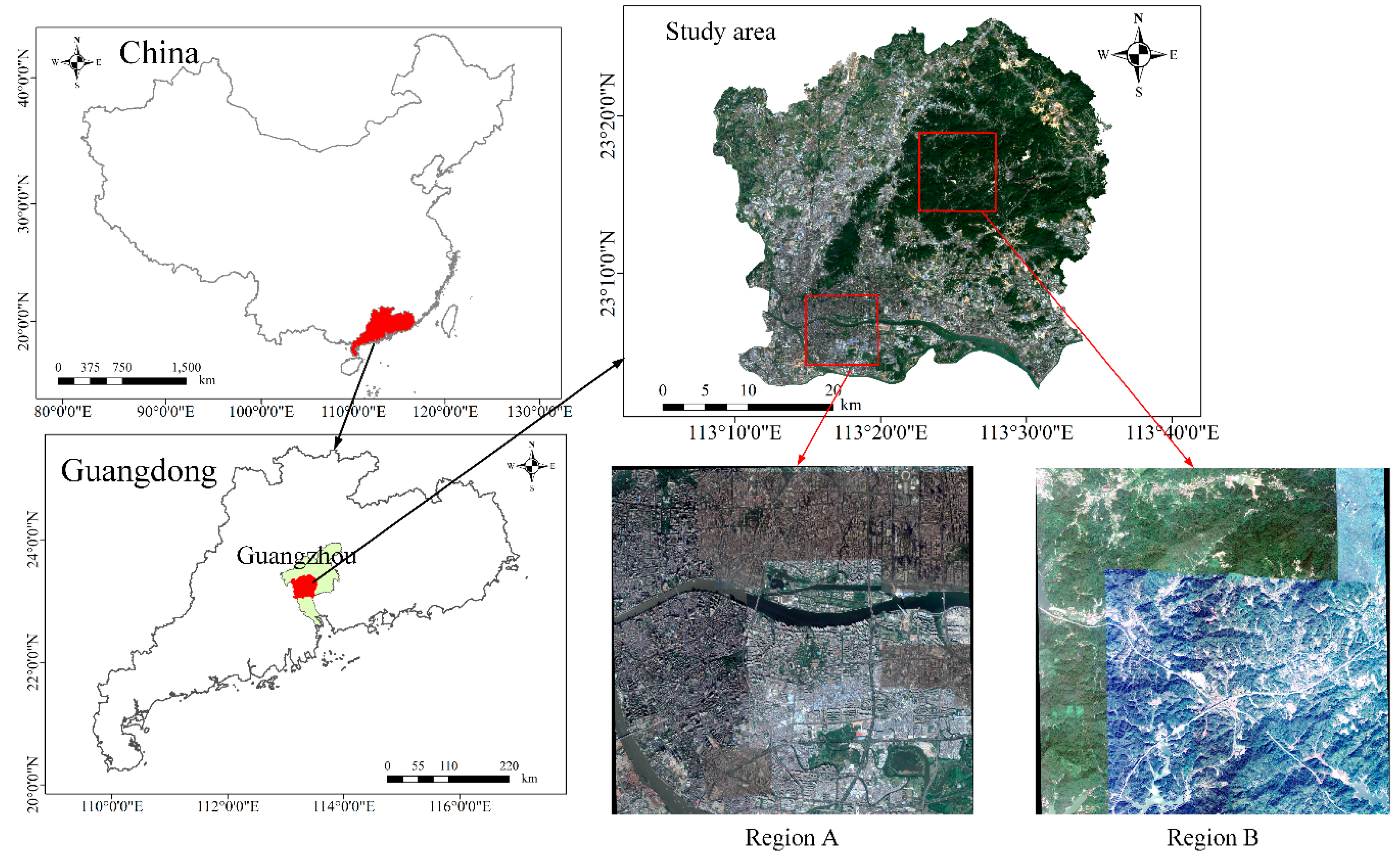
2.1. Study Area

Figure 1 shows the spatial distribution of the study areas. This study focuses on two typical urban areas with different land coverage patterns in Guangzhou city, China. The study areas consist of both built-up and forest areas, as shown in Figure 1. Guangzhou is situated in the Pearl River Delta hinterland, ranging from 22°26’ N to 23°56’ N, and from 112°57’ E to 114°30’ E. Guangzhou has a subtropical monsoon climate, which is characterized by mild winters and hot summers. The mean annual temperature range is 20–22 °C, and the mean precipitation is 1720 mm [42]. The maximum and minimum temperature in the study area reached 26.8 and 12.8℃ on 1 November 2017, respectively. The average daily temperature was 18.2℃ and the average daily relative humidity was about 72.3 percent. These study areas contained three types of land covers, i.e., impervious surfaces (containing building and road), vegetation, and water bodies. In Figure 1, region A is primarily covered by impervious surfaces, while region B is primarily covered by vegetation.

2.2. Data

ASTER is a multispectral scanner that produces images of high spatial resolutions of 15 to 90 m. It has three bands in the visible and near-infrared spectral range with a spatial resolution of 15 m, six bands in the shortwave-infrared spectral range with a spatial resolution of 30 m, and five bands in the thermal-infrared spectral range with a spatial resolution of 90 m. The ASTER LSTs were retrieved by using the temperature and emissivity separation method. The 90 m ASTER LST products (AST08) have an accuracy of about 1.5 K [43]. The product was obtained from NASA source (http://search.earthdata.nasa.gov) on 1 November 2017 and was projected to the UTM-49N (UTM: Universal Transverse Mercator, zone 49 N). The datum of projection is WGS_1984. In this study, the 90 m ASTER LST was rationally downscaled to 10 m.
In this study, the Sentinel-2A multispectral imagery with 0% cloud cover on 1 November 2017 was obtained from the Sentinels Scientific Data Hub (https://scihub.copernicus.eu/). The Sentinel-2A Level-1C (L1C) image was first preprocessed by radiometric and geometric corrections, which was geometrically rectified to UTM-49N. We used the Sen2Cor Atmospheric Correction Processor to derive the Sentinel-2A Level-2A (L2A) surface reflectance. The Sentinel Application Platform (SNAP, version 5.0) contained the Sen2Cor module. Thirteen spectral bands of Sentinel-2A L2A spectrum reflectance exist in the visible, near infrared, and shortwave infrared parts of the spectrum. In this study, L2A reflectance of bands 2, 3, 4, 8b, 11, and 12 were applied to the downscaling experiments. The 20 m reflectance of bands 11 and 12 were interpolated to 10 m using the nearest neighbor interpolation.
In the downscaling process, other land surface parameters that were retrieved from the 10 m Sentinel-2A image were also used, including impervious surface fraction, vegetation fraction, MNDWI, NDBI, and NDVI. The values of MNDWI [44], NDBI [45], and NDVI were calculated using the equations:
M N D W I = ρ G r e e n ρ S W I R 1 ρ G r e e n + ρ S W I R 1 ,
NDBI = ρ SWIR 1 ρ NIR ρ SWIR 1 + ρ NIR
N D V I = ρ N I R ρ R ρ N I R + ρ R .
where ρ G r e e n , ρ R , ρ N I R , and ρ S W I R 1 are the Sentinel-2A reflectance of bands 3, 4, 8b, and 11, respectively.
The 10 m urban impervious surface and vegetation fractions were extracted using the modified linear spectral mixture analysis (MLSMA) method with the Sentinel-2A imagery [41]. In MLSMA, the high-precision impervious surface and vegetation fractions were extracted by integrating the conventional LSMA and Otsu’s approaches with NDBI and NDVI. The process of extraction was described in detail in the research by Xu, Liu and Xu [41].

3. Methods

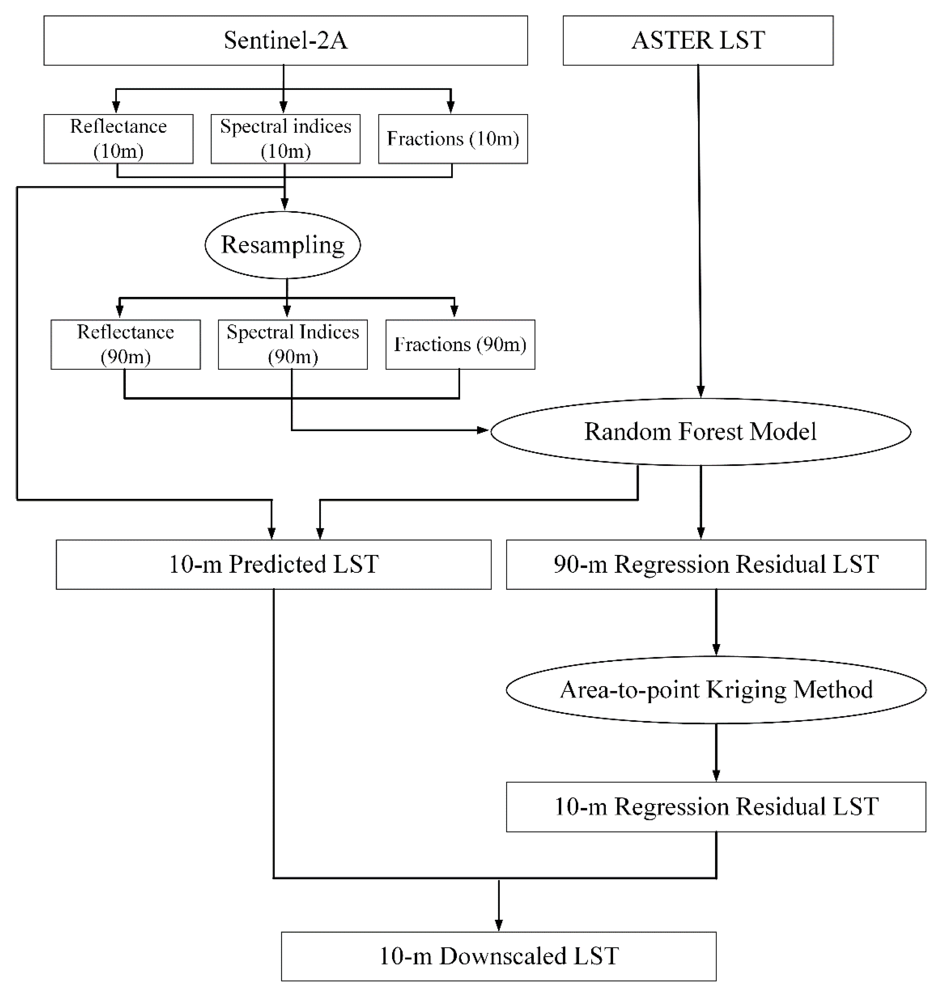
3.1. Downscaling Methodology

For downscaling the ASTER LST, twelve independent variables were used, including the reflectance of visible, near-infrared and short-wave infrared bands, NDVI, NDBI, MNDWI, impervious surface, soil and vegetation fractions, which were extracted from the Sentinel-2A imagery. The RFATPK downscaling procedure of integrating RF [46] and ATPK [47] methods was proposed to obtain the downscaled 10 m LST. The RFATPK considers the nonlinear relationship between LST and the land surface variables, and the spatial non-stationarity of residual LST estimated with the nonlinear regression model. The generic formulation of the RFATPK contains a trend component and a regression residual component, which is represented by the equation:
z ^ 10 m ( x ) = m ^ 10 m ( x ) +   ε ^ 10 m ( x )
where z ^ 10 m ( x ) is the final downscaled 10 m LST, m ^ 10 m ( x ) is the trend component estimated by RF, and ε ^ 10 m ( x ) is the regression residual component interpolated with ATPK. In the RFATPK, the LST spatial trend at the fine scale is first predicted with the RF-based regression model between LST and the independent variables; the regression residual LST is then downscaled using ATPK to obtain the fine residual LST prediction. Figure 2 shows the detailed flow diagram of the RFATPK downscaling procedure.

3.2. RF to Estimate the Spatial Trend

As a non-parametric ensemble learning method derived from the bagging algorithm, RF has been widely applied to classification and regression because of its high accuracy and insensitivity to multicollinearity [46]. RF is a combination of uncorrelated classification and decision regression tree predictors where each tree depends on the values of a random vector sampled independently and with the same distribution for all the trees in the forest. In this study, the RF regression method was implemented to enhance the spatial resolution of ASTER LST from 90 m to 10 m. The original ASTER LST was downscaled based on the nonlinear relationship with the independent variables estimated from Sentinel-2A imagery at 10 m resolution. Following the researches of Hutengs and Vohland [11], Duan and Li [29], and Li, Ni, Li, Duan and Wu [35], the 10 m spatial trend of ASTER LST was predicted using the RF-based regression method which is summarized as follows:
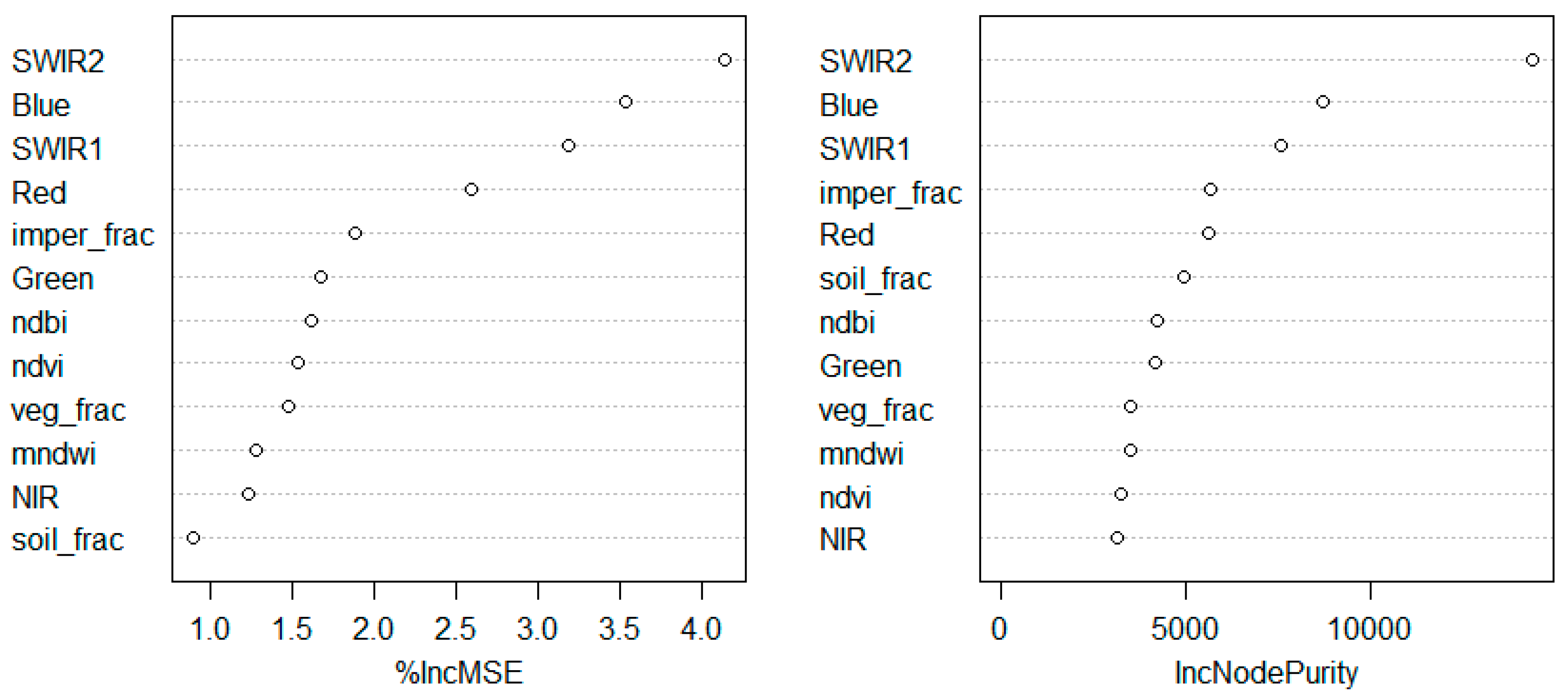
  • The independent variables with 10 m fine resolution, including the reflectance of blue, green and red bands, NIR, SWIR1 and SWIR2, NDVI, NDBI, MNDWI, impervious surface fraction, soil fraction, and vegetation fraction, were aggregated into the ASTER LST product with 90 m coarse resolution by using the spatial averaging method.
  • The multivariate nonlinear regression model between the 90 m ASTER LST and the aggregated independent variables could be established by using the RF algorithm, which can be expressed using the equation:
    m 90 m ( x ) =   RF ( b a n d s 90 m , N D V I 90 m ,   N D B I 90 m , M N D W I 90 m , f r a c 90 m   )  
    where m 90 m ( x ) is the 90 m ASTER LST, b a n d s 90 m represents the 90 m reflectance of visible and near-infrared and short-wave infrared bands, f r a c 90 m represents the 90 m impervious surface, soil, and vegetation fractions. The function RF ( · ) indicates the multivariate nonlinear regression model between ASTER LST and the independent variables constructed with the RF. The RF algorithm is implemented using an R package, randomForest.
  • The 10 m independent variables can be a direct input to the RF-based nonlinear regression model in Equation (5). Then, the downscaled spatial trend of LST at 10 m spatial resolution can be achieved.

3.3. ATPK for Downscaling the Residual LST

The coarse residual LST with a resolution of 90 m, also referred to as the model error of RF, was estimated through subtracting the RF-estimated LST from the 90 m ASTER LST. The residual LST at the coarse scale was, then, downscaled to the fine residual LST with a resolution of 10 m using the ATPK method [47]. ATPK ensures that the summation of the downscaled residual LST within any area is equivalent to the original coarse residual LST. In this study, the 90 m pixel is considered as an area, and the 10 m pixel is considered as a point. According to ATPK, the fine residual LST   ε ^ 10 m ( x ) of a given fine pixel x is estimated as a linear combination of the original coarse residual LSTs   ε 90 m ( v i ) in K neighboring coarse pixels, which can be represented by the equation:
  ε ^ 10 m ( x ) = i = 1 K λ x ( v i )   ε 90 m ( v i )
where   ε 90 m ( v i ) (i = 1, 2, 3, …, K) is the 90 m residual LST of the neighboring coarse pixel v i , and K is the number of neighboring coarse pixels used in the calculation of fine residual LST at fine pixel x. The λ x ( v i ) represents the ATPK weight of the coarse pixel v i and satisfies the condition j = 1 K λ x ( v j ) = 1 . The ATPK weights were estimated by minimizing the prediction error variance. The corresponding Kriging system of ATPK is represented by:
{ j = 1 K λ x ( v j ) C ¯ ( v i ,   v j ) + μ x = C ¯ ( v i ,   x ) ,       i = 1 , 2 , , K j = 1 K λ x ( v j ) = 1                                                                                                                                        
where μ x is the Lagrange multiplier, C ¯ ( v i ,   v j ) is the coarse-to-coarse covariance between the coarse pixels v i and v j , and C ¯ ( v i ,   x ) is the coarse-to-fine covariance between the coarse pixel v i and the fine pixel x. The calculations of the coarse-to-fine and coarse-to-coarse covariance terms are critical for downscaling the coarse residual LST in ATPK. First, the coarse pixel v i is discretized to N ( v i ) fine pixels, where the residual LST of the coarse pixel is assumed as the mean residual LST of the fine pixels within it.
C ¯ ( v i ,   x ) = 1 | v i | s v i C o v {   ε 10 m ( s ) ,   ε 10 m ( x ) } d s 1 N ( v i ) j = 1 N ( v i ) C ( s j ,   x ) ,   s j v i
C ¯ ( v i ,   v j ) = 1 | v i | 1 | v j | s v i s v j C o v {   ε 10 m ( s ) ,   ε 10 m ( s ) } d s d s 1 N ( v i ) 1 N ( v j ) k = 1 N ( v i ) l = 1 N ( v j ) C ( s k ,   s l ) ,   s k v i , s l v j
where C ( s j ,   x ) is the covariance between the fine pixels x and s j within the coarse pixel v i , and C ( s k ,   s l ) is the covariance between the fine pixel s k within the coarse pixel v i and the fine pixel s l within the coarse pixel v j . Then, the coarse-to-coarse and coarse-to-fine covariance terms can be estimated with the point-support semi-variogram, which was derived from the coarse residual LSTs using a deconvolution procedure [48,49]. The corresponding details can be referred from the research by Wang, et al. [50] and Wang, Shi, Atkinson and Pardo-Igúzquiza [48].

4. Results

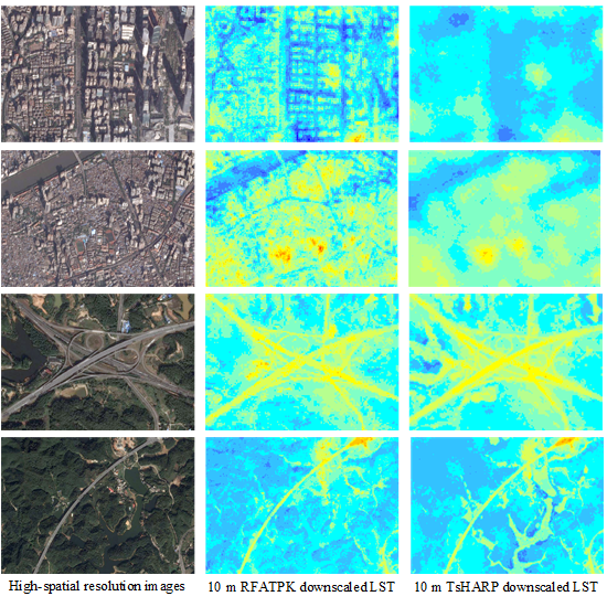
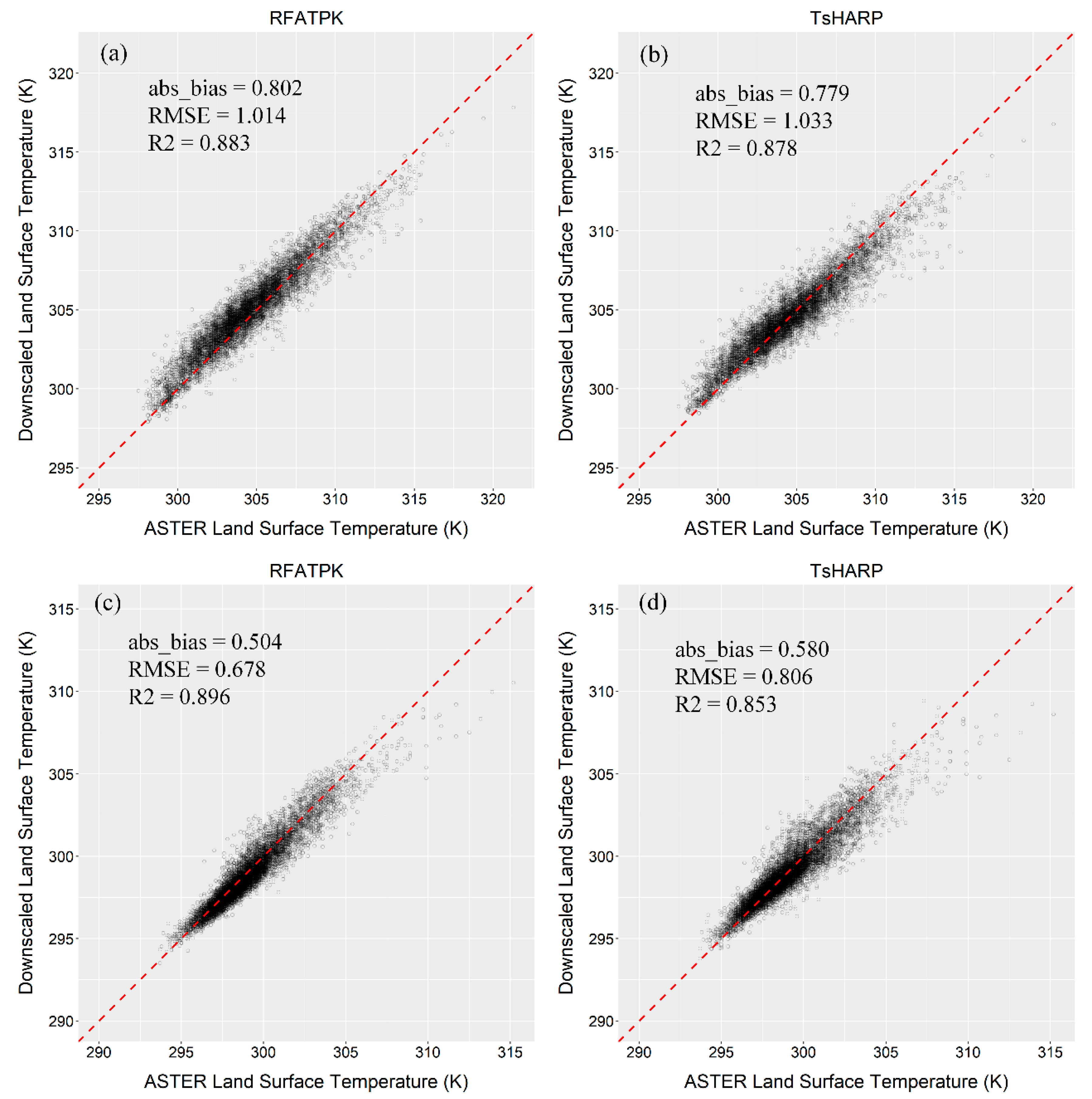
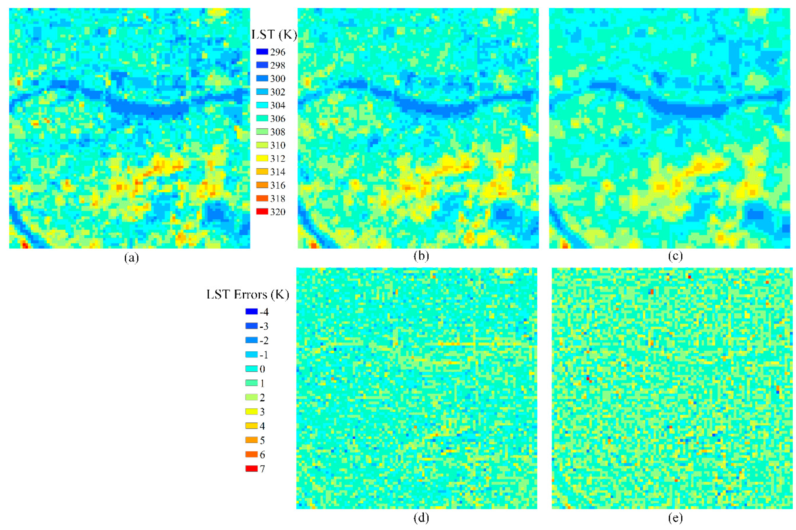
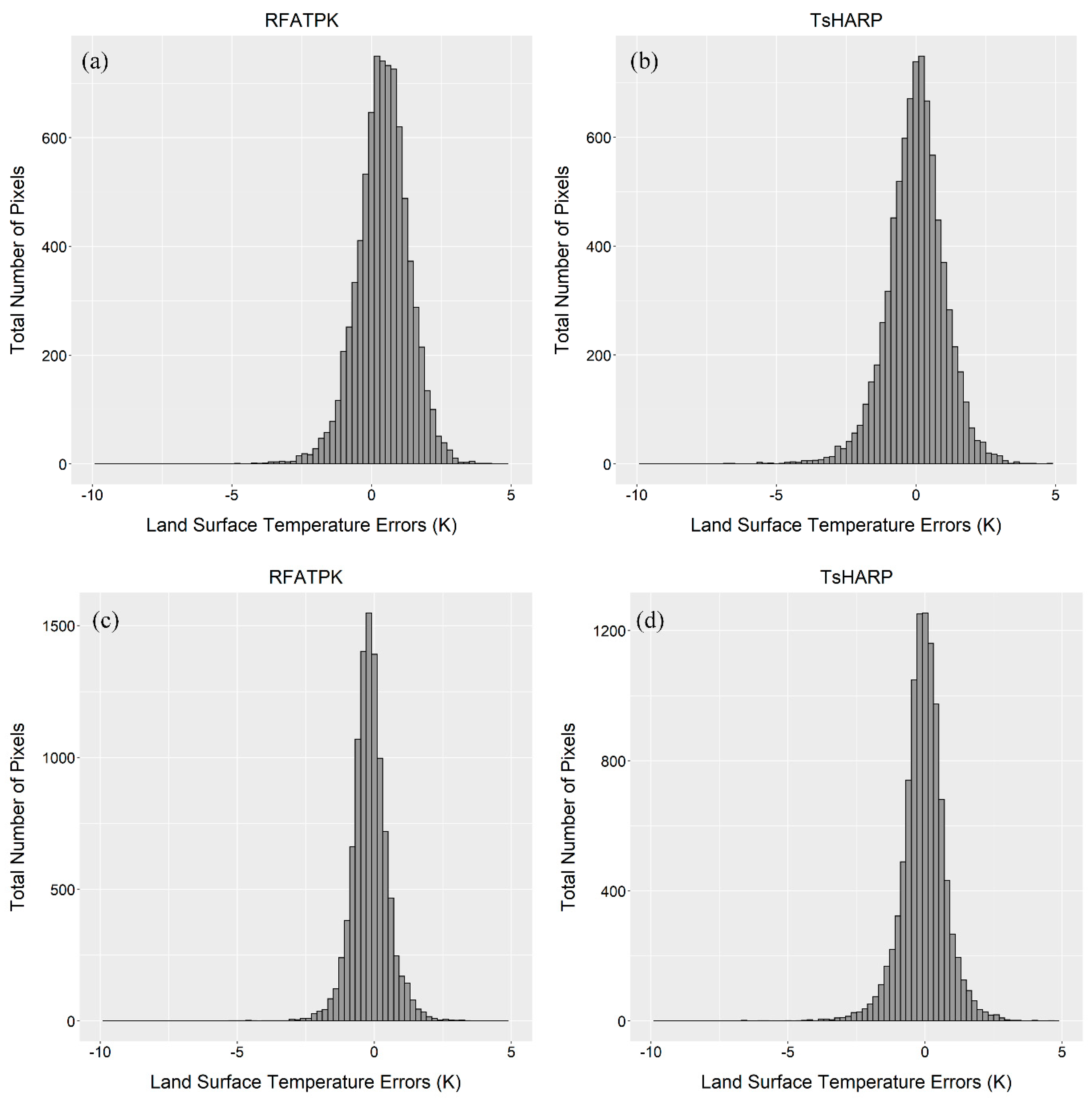
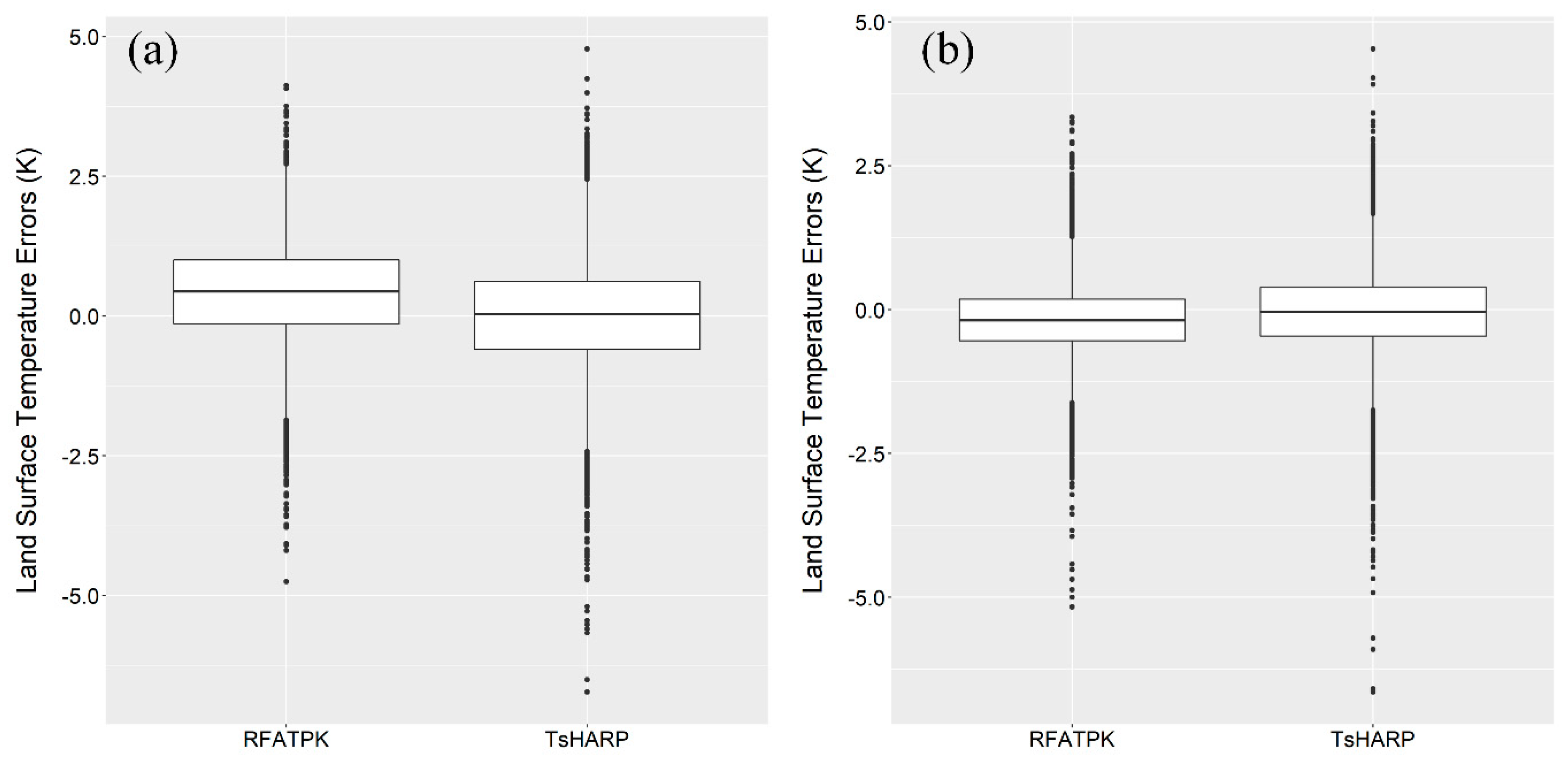
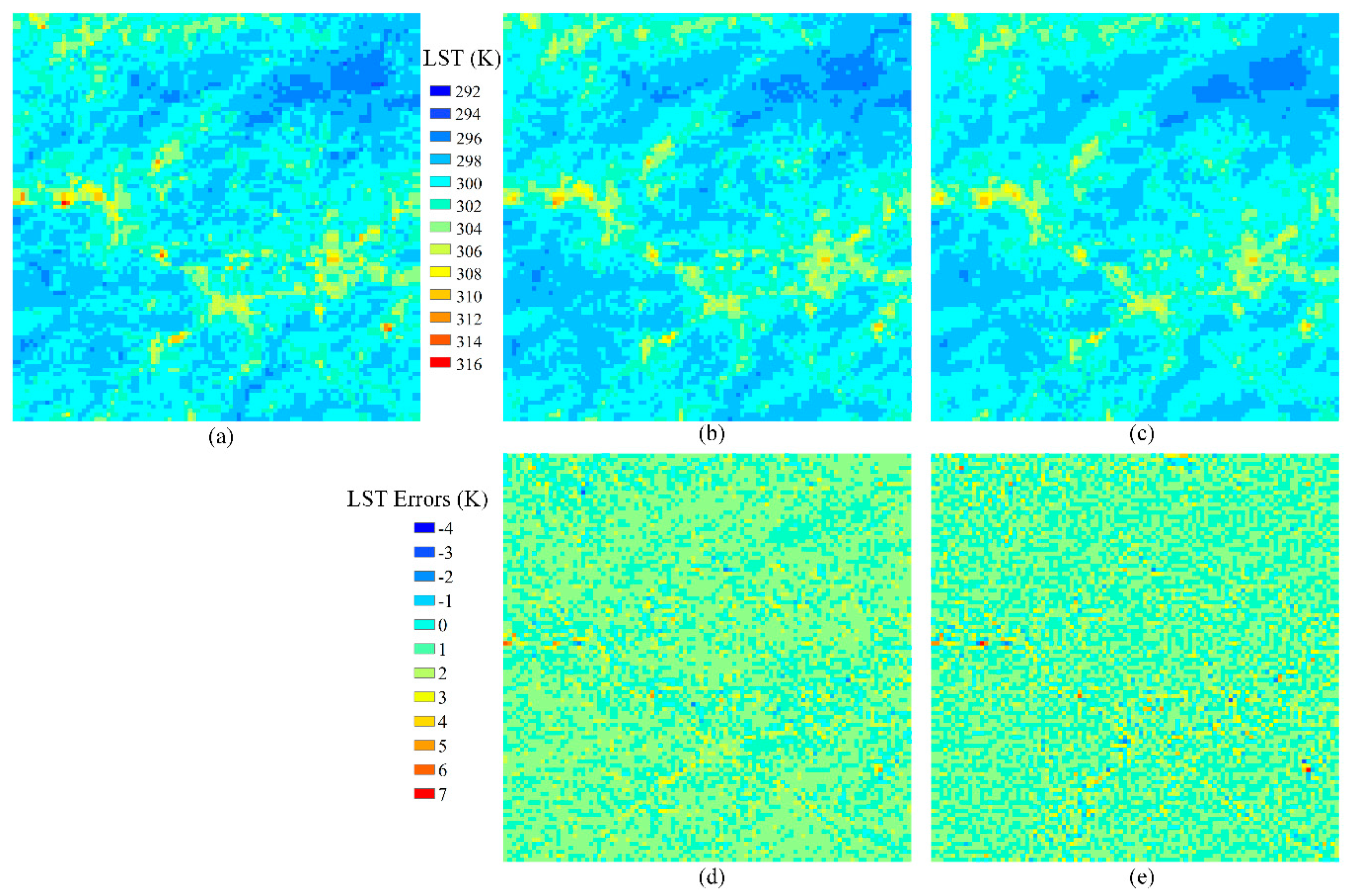
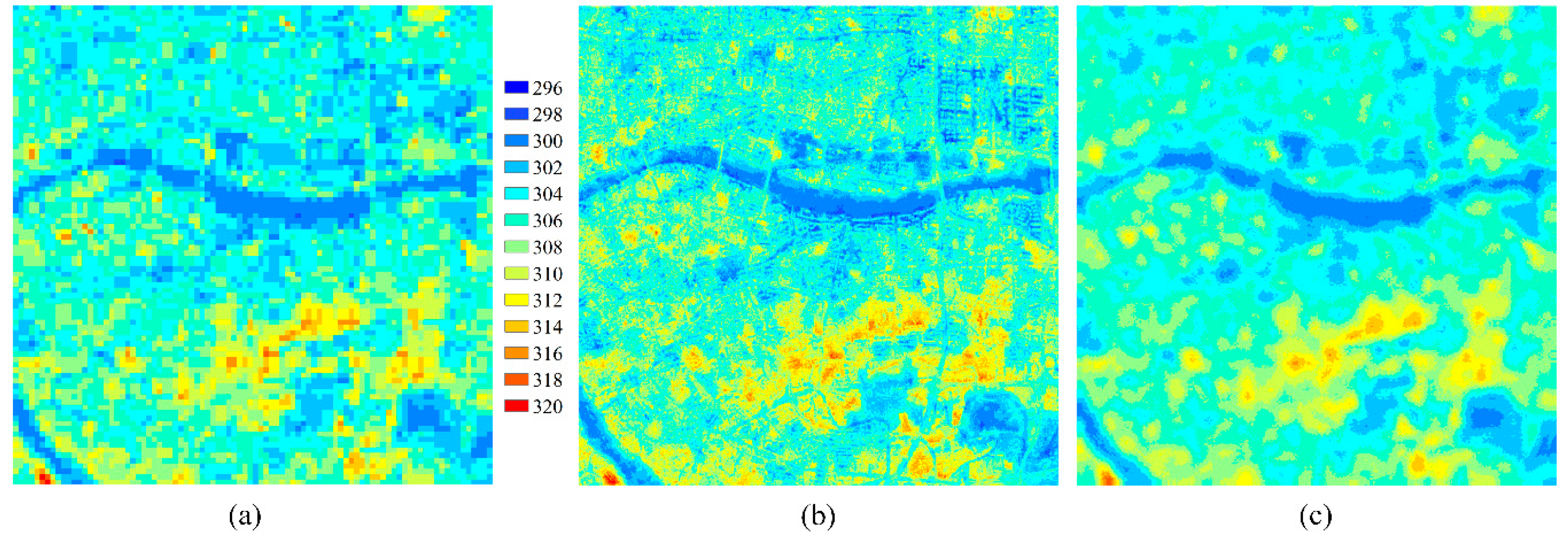
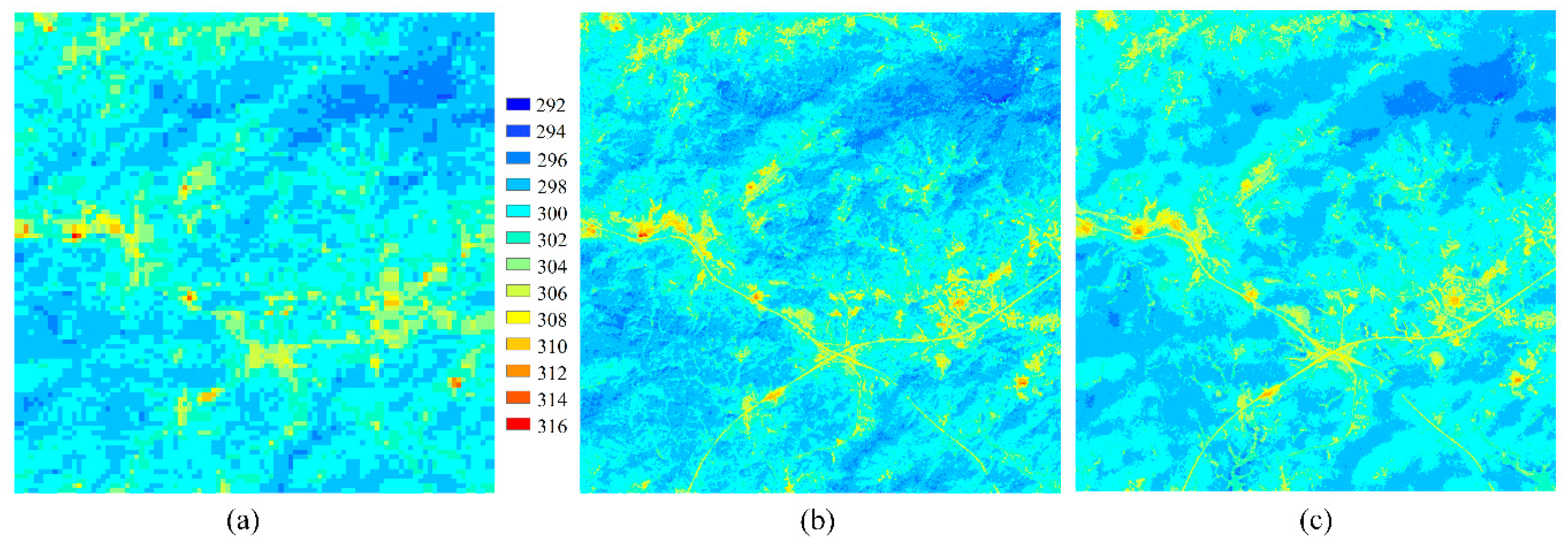
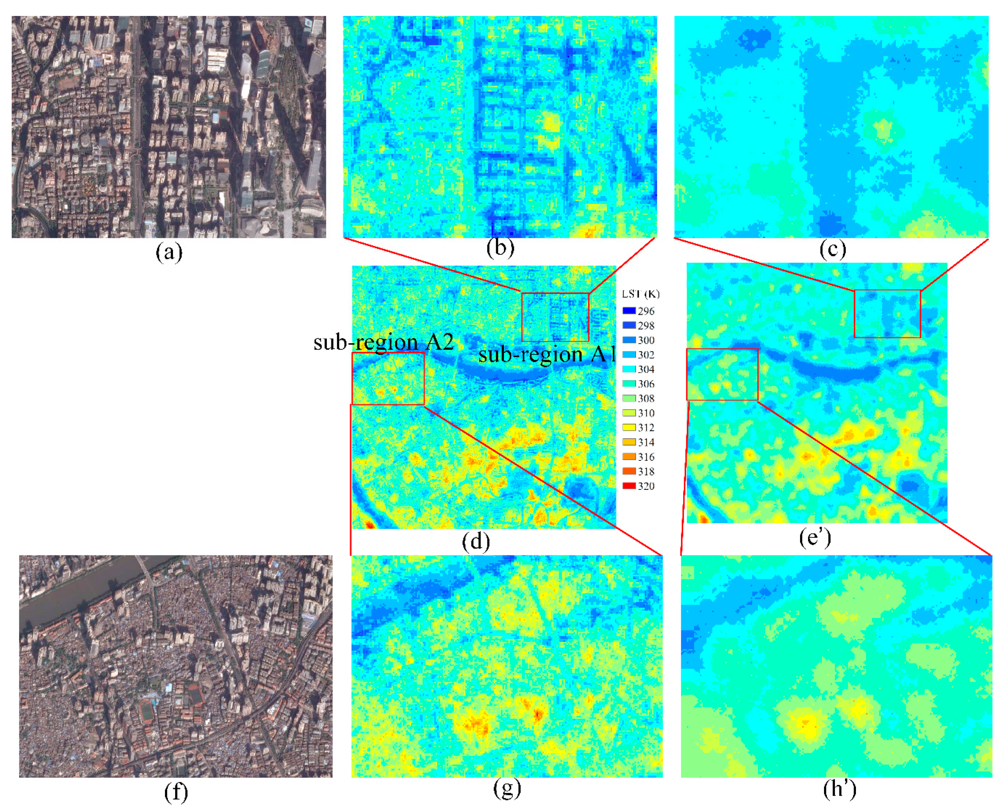
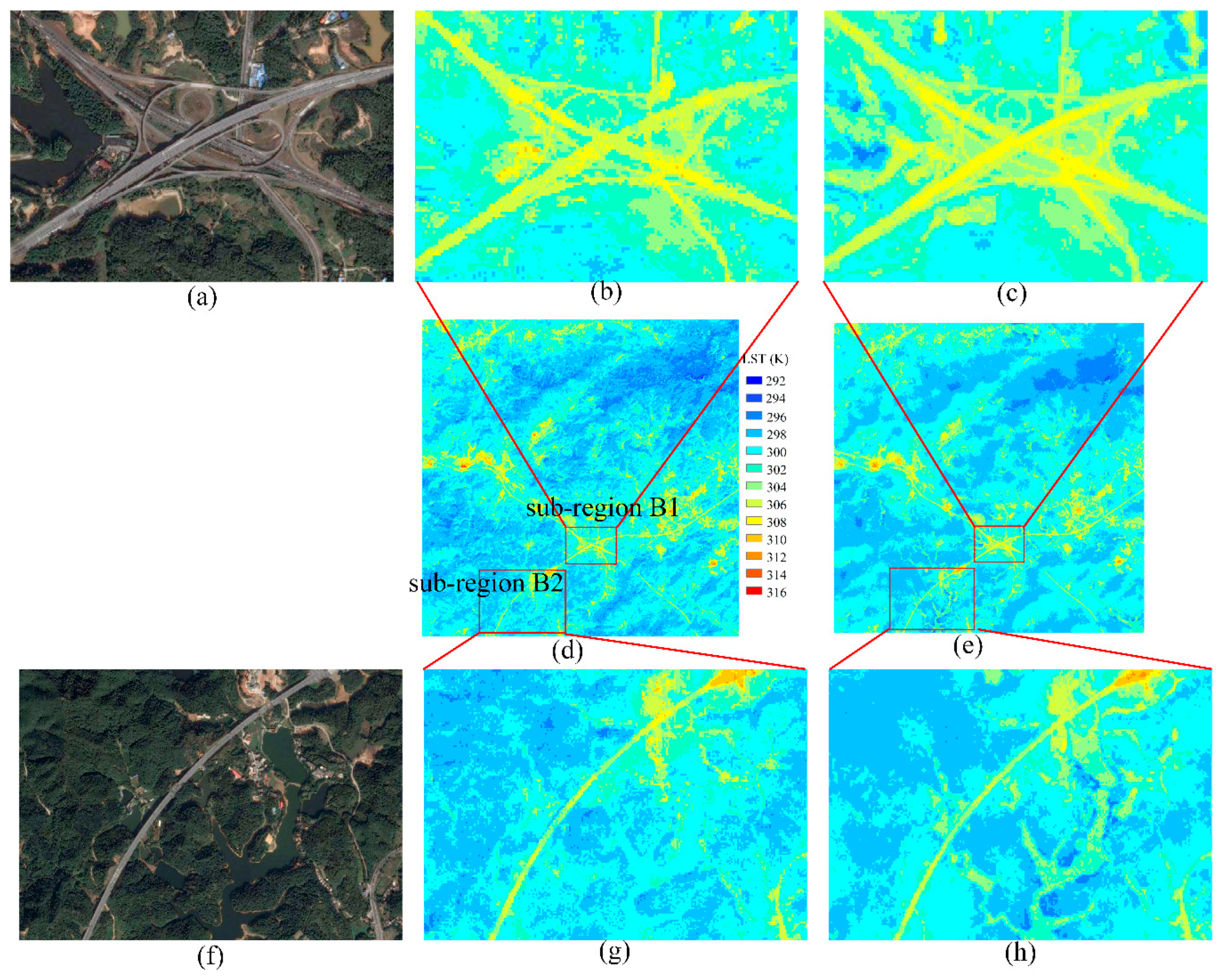
4.1. Downscaling Results

The 90 m ASTER LST on 1 November 2017 over two different land cover types were downscaled to 10 m using the RFATPK. In addition, the NDVI-based technique for spatial sharpening of thermal imagery proposed by Agam, Kustas, Anderson, Li and Neale [17] was also applied to downscale the ASTER LST. The RFATPK and the TsHARP were programmed with R Language, and the RF was performed with the R-based randomForest package (https://cran.r-project.org/web/packages/randomForest/index.html). To evaluate the downscaling performance of the RFATPK and the TsHARP, the downscaled results were upscaled to 90 m by using the spatial averaging method, and then validated by the original 90 m ASTER LST. In this study, three measures, including absolute bias (abs_bias), root mean square error (RMSE), and the coefficient of determination (R2), were chosen for the accuracy assessment of the downscaled LSTs and are shown in Figure 3.
In Figure 3, the RFATPK with the lowest RMSE and the highest R2 outperforms the TsHARP in regions A and B. In region A, the RFATPK had the lowest RMSE of 1.014 K and the highest R2 of 0.883, while its absolute bias was about 0.023 K greater than the TsHARP. In the region B, the absolute bias was reduced from 0.580 K of the TsHARP to 0.504 K of the RFATPK, and RMSE was reduced from 0.806 K to 0.678 K, which presents a 15.88% improvement in the magnitude of the downscaling results with the RFATPK. The R2 of the RFATPK reached 0.896, approximately 0.043 higher than the TsHARP. On the basis of these results, the RFATPK displayed better overall downscaling performance than the TsHARP in both regions A and B, although the absolute bias of the RFATPK is larger than that of the TsHARP in region A.
Figure 3 also shows the scatterplot comparisons of the 90 m ASTER and aggregated LSTs from the downscaled results of the RFATPK and the TsHARP. The RFATPK showed an improvement in the downscaling performance as compared with the TsHARP, with an overall reduced scatter around the 1:1 line (Figure 3). However, an overestimation of low LST extremes and an underestimation of high LST extremes was identified in both the methods in both the regions. The high LST extremes of the TsHARP tend to diverge around the 1:1 line in both the study areas, while the RFATPK produced more aggregation of the high LST extremes. Figure 3 also shows that overall, the RFATPK overestimates the downscaled LSTs in region A, mainly covered by built-up, and underestimates the downscaled LSTs in region B mainly covered by forests. The RFATPK performed better in downscaling ASTER LST, with a greater R2 and a smaller RMSE, in region B than that in region A, as a result of the spatial heterogeneity of land cover types, which led to spatial changes in the LSTs of different regions. The spatial patterns of region A, which was mainly covered by built-up, were more complicated than that of region B, which was mainly covered by forests. Nevertheless, the RFATPK showed high capacity for downscaling LST in these regions covered by different land cover types.
Figure 4 shows the spatial distribution of 90 m downscaled LSTs, and Figure 5a,b presents the error distributions of downscaled LSTs for region A with the RFATPK and the TsHARP. Compared to the 90 m ASTER LST in Figure 4a, the RFATPK and the TsHARP downscaled LSTs shown in Figure 4b,c, both had similar spatial distributions as that of the original ASTER LST. TsHARP showed slightly better performance than the RFATPK with an absolute bias of 0.779 K (Figure 3b). The LST errors of the TsHARP were concentrated to a value of 0, while the LST errors of the RFATPK tended to be greater than 0, as shown in Figure 5a,b) and Figure 6a. However, the TsHARP had the maximum and minimum LST errors of 5.0 K and −5.0 K, respectively, which performed worse than the RFATPK. Furthermore, the RFATPK showed more detailed information of the downscaled LST and the TsHARP had a smoothing effect on the downscaled LST, as shown in Figure 4. The high LST extremes of the RFATPK are closer to the original ASTER LST extremes than that of the TsHARP.
The error distributions of the downscaled LSTs from the RFATPK and the TsHARP, and the spatial distribution of the 90 m downscaled LSTs in region B are shown in Figure 5c,d, Figure 6b, and Figure 7, respectively. The RFATPK, with lesser absolute bias and RMSE (highlighted in Figure 3c,d), produced smaller LST errors in the downscaling process than the TsHARP, as shown in Figure 5c,d, and Figure 6b. This indicates that the RFATPK displays better downscaling performance than the TsHARP. The RFATPK downscaled LST showed a similar spatial distribution to that of the original ASTER LST, as shown in Figure 7. The RFATPK captured more details in the downscaled LST image, while spatial details were lost in the TsHARP resulting in smoother LST extremes. This further led to an underestimation of downscaled LSTs with high extreme values.
The 90 m ASTER LST over different land cover types was downscaled to 10 m using the RFATPK and the TsHARP. The 10 m downscaled LSTs of the RFATPK and the TsHARP in regions A and B are shown in Figure 8 and Figure 9, respectively. The 10 m downscaled LSTs showed a similar but more detailed spatial distribution as compared with the 90 m ASTER LST. This indicates that both the RFATPK and the TsHARP captured the details of LST images in the downscaling process. The RFATPK captured the complicated nonlinear relationship between the LST and independent variables more precisely by introducing multiple-type independent variables, including the reflectance of visible and near-infrared and short-wave infrared bands, NDVI, NDBI, MNDWI, impervious surface, soil, and vegetation fractions. As a result, the RFATPK produced a more detailed 10 m LST, and performed better than the TsHARP, as shown in Figure 8 and Figure 9. On the basis of the relationship between LST and NDVI, the TsHARP only considers a single independent variable; thus, is more inclined to have the potential losses of LST details. Figure 8c and Figure 9c also show a smoothing effect on the spatial distribution of 10 m TsHARP LST. This presents that the TsHARP lost the details of downscaled LST, especially in the built-up areas of region A. In these areas of region A, the RFATPK effectively differentiated the LSTs of buildings, road, water, and vegetation, as shown in Figure 8, while the TsHARP lost the spatial difference features of building and vegetation LSTs because of smoothing.

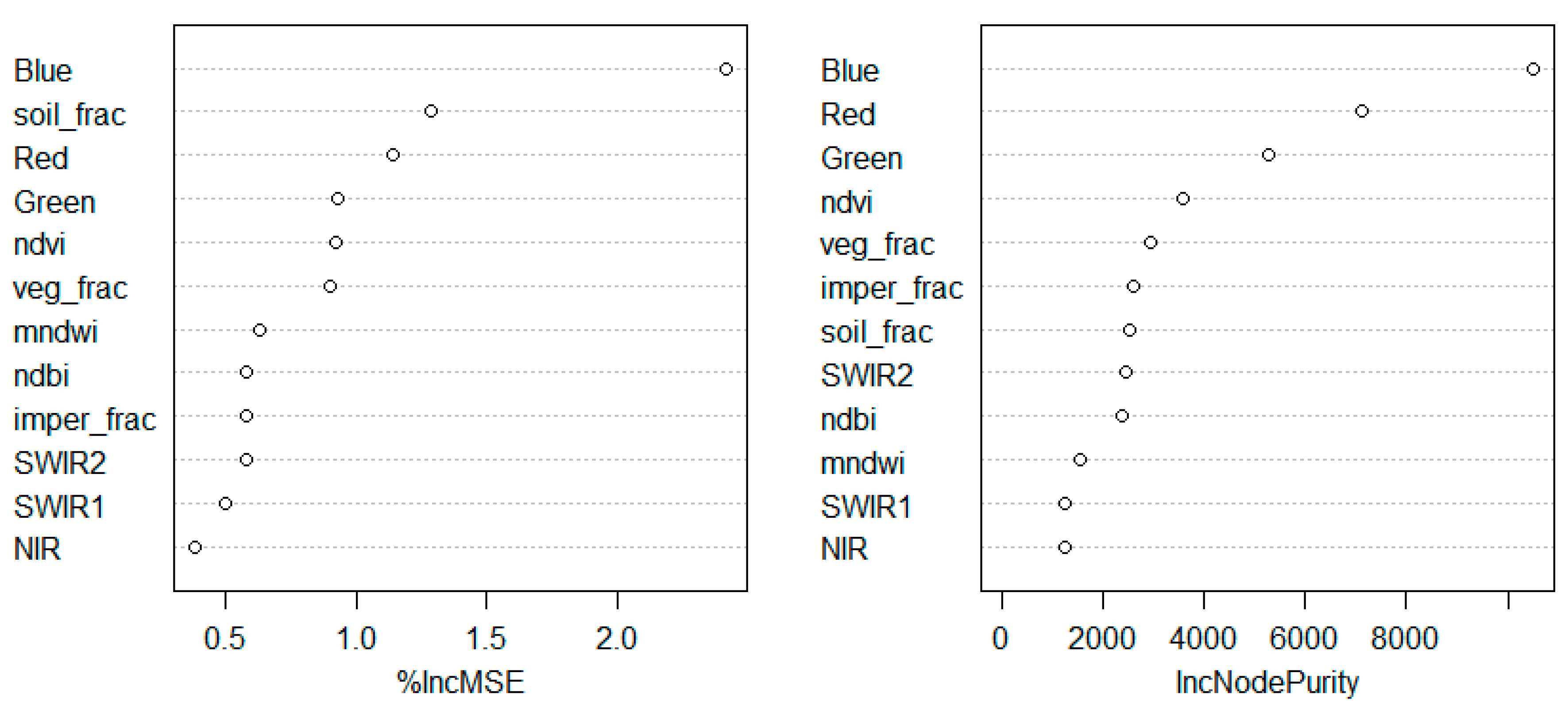
4.2. Variable Importance Analysis

In this study, mean decrease accuracy (%IncMSE) and mean decrease Gini (IncNodePurity) were used to analyze the importance of the independent variables in regions A and B. The %IncMSE indicates the increase in the mean squared error (MSE) of prediction, and the IncNodePurity is used to measure quality of a split for every variable of a tree by means of the Gini index. The importance of the independent variables reflects their contribution to the regression model. The importance of each independent variable for regions A and B is highlighted in Figure 10 and Figure 11.
The contributions of spectral reflectance, especially from SWIR2, blue, SWIR1, and red bands, were the highest in region A, as shown in Figure 10. Furthermore, impervious surface fraction had the highest importance because of its greater contribution to the downscaled ASTER LST than vegetation and soil fraction, while soil fraction was the least important. This implies that, other than spectral reflectance, impervious surface fraction and soil fraction were the most and least significant variables, respectively, when downscaling ASTER LST in the built-up-dominated region A. In fact, this is appropriate because region A was mainly covered by impervious surfaces, with very few soil regions. Furthermore, there is a significant correlation between LST and impervious surfaces in the built-up-dominated urban environment. Therefore, the soil fraction variable can be discarded in the downscaling process of ASTER LST in region A.
In Figure 11, the importance of independent variables in region B was significantly different because of the forest areas. Figure 11 also shows the importance of each independent variable in region B. In general, blue reflectance, soil fraction, red reflectance, green reflectance, NDVI, and vegetation fraction are six of the most important variables, with their importance scores (IncMSE) greater than one. This indicates that these variables were the most significant when downscaling ASTER LST in region B. In addition to spectral reflectance, soil fraction, NDVI, and vegetation fraction were the most important contributors to LST in the forest-dominated region B. Furthermore, because the region was primarily covered by vegetation and soil, contributions from the building variables were low, especially from NDBI and impervious surface fraction, as shown in Figure 11. In the future, the relevant variables associated with vegetation and soil should be selected to downscale the LST in the corresponding regions.

5. Discussion

To explore the downscaling performance of the RFATPK and the TsHARP, the 10 m downscaled LSTs in regions A and B with different land cover patterns were further analyzed with Google Maps, as shown in Figure 12 and Figure 13.
The LST over building roofs was higher than that of the roads, as shown in Figure 12a,b, because portions of the roads were covered by plants. The LST in the green belts surrounding the buildings was significantly lower than that of roads. These results show that different land cover types cause different heating and cooling effects. Land areas, blanketed with impervious surfaces such as buildings and roads, are the main contributors to urban heat islands, while vegetation has a good effect of lowering the LST. Figure 12b also shows that the land areas covered by building shadows in subregion A1 have a low LST because of the cooling effect from these shadows. However, the TsHARP did not capture these details because of its smoothing effect, as shown in Figure 12c.
In subregion A2, as shown in Figure 12g,h, the RFATPK effectively retrieved the LSTs for the regions of buildings, water bodies, and roads. The low-density building regions had low overall LSTs than the high-density building regions, as shown in Figure 12b,g, probably because of the vegetation fraction and the spatial distribution of impervious surfaces. The LSTs of water bodies were lower than those of buildings and roads. Furthermore, the RFATPK differentiated between the LSTs of the bridges over rivers and the water bodies, where the LST of bridges was significantly higher than that of water bodies. However, these LSTs retrieved by the TsHARP were closer to that of water bodies. Because it was improbable that bridges, which are mainly composed of concrete impervious surfaces, had a positive effect on LST, and the water bodies generally have a good effect of cooling down the temperature, it was determined that the TsHARP overestimated the LST of water bodies.
The spatial distributions of the 10 m downscaled LST from the TsHARP and the RFATPK were similar in the road and forest regions, while they were obviously different over water bodies, as shown in Figure 13c,h. The TsHARP captured a higher LST for the water bodies than the RFATPK, whose value was closer to that of roads and soils (Figure 13h). The overestimation of the LST of water bodies by the TsHARP was attributed to its NDVI-based function. The TsHARP can be represented mathematically [17] using the equation LST = A + B   × ( 1   NDVI ) 0.625 . In general, an NDVI value of less than 0 indicates a water pixel, and these pixels have a larger value for ( 1   NDVI ) 0.625 . This results in the overestimation of LST for the water pixels with the same values of the coefficients A and B in a whole image. These experimental results show that the application of the TsHARP is limited while downscaling the LST for land areas blanketed with water bodies.
Overall, the RFATPK was more practical in downscaling the 90 m ASTER LST to 10 m LST by incorporating spectral reflectance of Sentinel-2A image, spectral indices, and fractions of impervious surface, soil, and vegetation. Furthermore, the RFATPK considered the nonlinear relationship between LSTs and independent variables and the scale effect of the regression residual LST on the downscaling process of ASTER LST. However, large errors were found in the downscaled LSTs, especially at the LST pixel extremes. This could be because RF, which in essence is a non-spatial method for spatial trend prediction, ignores the spatial locations and patterns of samples. This could potentially lead to overestimating or underestimating the LST spatial trend during the downscaling process. A more reasonable geostatistical theory-based ML method could be applied for downscaling the LST from different remote sensing data by considering the geographical proximity and spatial relations between the LST pixels [51]. Furthermore, in the future, additional parameters could be used to precisely downscale the LSTs by completely defining the nonlinear relationship between LST and these parameters, including high-resolution building density, building height, DEM, albedo, sky views, and different spectral indices such as BSI, DVI, SAVI, and IBI [28].

6. Conclusions

In this study, an ML-based geostatistical downscaling method (RFATPK) was proposed, which integrates the advantages of both RF and ATPK methods. Then, this method was applied to downscale 90 m ASTER LST data to 10 m in two typical regions in Guangzhou, China. The spectrum reflectance of different bands, NDVI, NDBI, MNDWI, impervious surface, and vegetation fractions derived from Sentinel-2A imagery dated 1 November 2017 were used as the independent variables in this method. The downscaled results were, then, compared with the NDVI-based thermal sharpening method (TsHARP). The major conclusions are as follows:
The RFATPK which considered multi-type independent variables, was better than the TsHARP which considered only a single variable. On the basis of the statistical relationship between LST and NDVI, the TsHARP assumes that LST is mainly influenced by vegetation. Furthermore, the TsHARP does not account for the correlation between LST and impervious surfaces and water bodies. This could result in large errors in the LST of complex urban regions, especially in the regions containing water bodies. By considering multi-type independent variables, the RFATPK captured LST difference over different land cover types and produced the spatial details of high-resolution downscaled LST in heterogeneous urban regions.
Although the RFATPK can produce precise 10 m LST with more spatial details by downscaling the 90 m ASTER LST, its validity could be further tested by downscaling the LST from different remote sensing data. Furthermore, there remains a large error in the downscaled LSTs, especially at the LST extremes. In the downscaling process, the RFATPK does not consider the spatial autocorrelation and spatial locations of LST image, which tends to underestimate the high LST values and overestimate the low LST values. In future studies, other factors, for example, high-resolution building height, albedo, and sky views related to urban LST could be investigated in the downscaling process. The results can potentially contribute to improving our understanding of heat exchange processes in urban environments and has wide contributions in meteorological, hydrological, and ecological research [52].

Author Contributions

J.X. and F.Z. designed the experimental framework and wrote the draft manuscript; J.X, H.H., and H.J. collected data and implemented the experiments; H.J. and W.J. analyzed the results; K.Z., J.Y. and B.J. reviewed the manuscript and gave suggestions for improving the manuscript. All authors have read and have read and agreed the final manuscript.

Funding

This research is jointly funded by the Science and Technology Planning Project of Guangdong Province (nos. 2018B020207012 and 2018B020207002), the National Natural Science Foundation of China (no. 41901371), the Key Special Project for Introduced Talents Team of Southern Marine Science and Engineering Guangdong Laboratory (Guangzhou) (no. GML2019ZD0301), the Guangdong Innovative and Entrepreneurial Research Team Program (no. 2016ZT06D336), the GDAS’ Project of Science and Technology Development (nos. 2018GDASCX-0101 and 2019GDASYL-0302001), the open fund of Key Lab of Guangdong for Utilization of Remote Sensing and Geographical Information System (no. 2017B030314138), and the Provincial Agricultural Science and technology innovation and promotion project of Guangdong Province (no. 2019KJ147).

Acknowledgments

We would like to thank the anonymous reviewers and the editor for providing valuable suggestions and comments, which have greatly improved this manuscript.

Conflicts of Interest

The authors declare no conflict of interest.

References

  1. Voogt, J.A.; Oke, T.R. Thermal remote sensing of urban climates. Remote Sens. Environ. 2003, 86, 370–384. [Google Scholar] [CrossRef]
  2. Li, Z.; Tang, B.; Wu, H.; Ren, H.; Yan, G.; Wan, Z.; Trigo, I.F.; Sobrino, J.A. Satellite-derived land surface temperature: Current status and perspectives. Remote Sens. Environ. 2013, 131, 14–37. [Google Scholar] [CrossRef] [Green Version]
  3. Kustas, W.P.; Anderson, M.C. Advances in thermal infrared remote sensing for land surface modeling. Agric. For. Meteorol. 2009, 149, 2071–2081. [Google Scholar] [CrossRef]
  4. Lazzarini, M.; Marpu, P.R.; Ghedira, H. Temperature-land cover interactions: The inversion of urban heat island phenomenon in desert city areas. Remote Sens. Environ. 2013, 130, 136–152. [Google Scholar] [CrossRef]
  5. Yao, R.; Wang, L.; Huang, X.; Niu, Z.; Liu, F.; Wang, Q. Temporal trends of surface urban heat islands and associated determinants in major Chinese cities. Sci. Total Environ. 2017, 609, 742–754. [Google Scholar] [CrossRef]
  6. Mutiibwa, D.; Strachan, S.; Albright, T.P. Land Surface Temperature and Surface Air Temperature in Complex Terrain. IEEE J. Sel. Top. Appl. Earth Obs. Remote Sens. 2015, 8, 4762–4774. [Google Scholar] [CrossRef]
  7. Wang, Y.; Hu, B.K.H.; Myint, S.W.; Feng, C.; Chow, W.T.L.; Passy, P. Patterns of land change and their potential impacts on land surface temperature change in Yangon, Myanmar. Sci. Total Environ. 2018, 643, 738–750. [Google Scholar] [CrossRef]
  8. Yin, C.; Yuan, M.; Lu, Y.; Huang, Y.; Liu, Y. Effects of urban form on the urban heat island effect based on spatial regression model. Sci. Total Environ. 2018, 634, 696–704. [Google Scholar] [CrossRef]
  9. Zawadzka, J.; Corstanje, R.; Harris, J.A.; Truckell, I. Downscaling Landsat-8 land surface temperature maps in diverse urban landscapes using multivariate adaptive regression splines and very high resolution auxiliary data. Int. J. Digit. Earth 2019. [Google Scholar] [CrossRef] [Green Version]
  10. Lo, C.P.; Quattrochi, D.A.; Luvall, J.C. Application of high-resolution thermal infrared remote sensing and GIS to assess the urban heat island effect. Int. J. Remote Sens. 1997, 18, 287–304. [Google Scholar] [CrossRef] [Green Version]
  11. Hutengs, C.; Vohland, M. Downscaling land surface temperatures at regional scales with random forest regression. Remote Sens. Environ. 2016, 178, 127–141. [Google Scholar] [CrossRef]
  12. Zhan, W.; Chen, Y.; Zhou, J.; Li, J.; Liu, W. Sharpening Thermal Imageries: A Generalized Theoretical Framework From an Assimilation Perspective. IEEE Trans. Geosci. Remote Sens. 2011, 49, 773–789. [Google Scholar] [CrossRef]
  13. Zaksek, K.; Ostir, K. Downscaling land surface temperature for urban heat island diurnal cycle analysis. Remote Sens. Environ. 2012, 117, 114–124. [Google Scholar] [CrossRef]
  14. Zhang, X.; Zhao, H.; Yang, J. Spatial downscaling of land surface temperature in combination with TVDI and elevation. Int. J. Remote Sens. 2019, 40, 1875–1886. [Google Scholar] [CrossRef]
  15. Bisquert, M.; Sanchez, J.M.; Caselles, V. Evaluation of Disaggregation Methods for Downscaling MODIS Land Surface Temperature to Landsat Spatial Resolution in Barrax Test Site. IEEE J. Sel. Top. Appl. Earth Obs. Remote Sens. 2016, 9, 1430–1438. [Google Scholar] [CrossRef]
  16. Kustas, W.P.; Norman, J.M.; Anderson, M.C.; French, A.N. Estimating subpixel surface temperatures and energy fluxes from the vegetation index-radiometric temperature relationship. Remote Sens. Environ. 2003, 85, 429–440. [Google Scholar] [CrossRef]
  17. Agam, N.; Kustas, W.P.; Anderson, M.C.; Li, F.; Neale, C.M.U. A vegetation index based technique for spatial sharpening of thermal imagery. Remote Sens. Environ. 2007, 107, 545–558. [Google Scholar] [CrossRef]
  18. Dominguez, A.; Kleissl, J.; Luvall, J.C.; Rickman, D.L. High-resolution urban thermal sharpener (HUTS). Remote Sens. Environ. 2011, 115, 1772–1780. [Google Scholar] [CrossRef] [Green Version]
  19. Essa, W.; Verbeiren, B.; Der Kwast, J.V.; De Voorde, T.V.; Batelaan, O. Evaluation of the DisTrad thermal sharpening methodology for urban areas. Int. J. Appl. Earth Obs. Geoinf. 2012, 19, 163–172. [Google Scholar] [CrossRef]
  20. Agam, N.; Kustas, W.P.; Anderson, M.C.; Li, F.; Colaizzi, P.D. Utility of thermal image sharpening for monitoring field-scale evapotranspiration over rainfed and irrigated agricultural regions. Geophys. Res. Lett. 2008, 35, L02402. [Google Scholar] [CrossRef] [Green Version]
  21. Chen, X.; Li, W.; Chen, J.; Rao, Y.; Yamaguchi, Y. A Combination of TsHARP and Thin Plate Spline Interpolation for Spatial Sharpening of Thermal Imagery. Remote Sens. 2014, 6, 2845–2863. [Google Scholar] [CrossRef] [Green Version]
  22. Inamdar, A.K.; French, A.N. Disaggregation of GOES land surface temperatures using surface emissivity. Geophys. Res. Lett. 2009, 36, L02408. [Google Scholar] [CrossRef]
  23. Mukherjee, S.; Joshi, P.K.; Garg, R.D. Regression-Kriging Technique to Downscale Satellite-Derived Land Surface Temperature in Heterogeneous Agricultural Landscape. IEEE J. Sel. Top. Appl. Earth Obs. Remote Sens. 2015, 8, 1245–1250. [Google Scholar] [CrossRef]
  24. Fasbender, D.; Tuia, D.; Bogaert, P.; Kanevski, M. Support-Based Implementation of Bayesian Data Fusion for Spatial Enhancement: Applications to ASTER Thermal Images. IEEE Geosci. Remote Sens. Lett. 2008, 5, 598–602. [Google Scholar] [CrossRef]
  25. Bonafoni, S. Downscaling of Landsat and MODIS Land Surface Temperature over the Heterogeneous Urban Area of Milan. IEEE J. Sel. Top. Appl. Earth Obs. Remote Sens. 2016, 9, 2019–2027. [Google Scholar] [CrossRef]
  26. Bonafoni, S.; Anniballe, R.; Gioli, B.; Toscano, P. Downscaling Landsat Land Surface Temperature over the urban area of Florence. Eur. J. Remote Sens. 2016, 49, 553–569. [Google Scholar] [CrossRef]
  27. Peng, Y.; Li, W.; Luo, X.; Li, H. A Geographically and Temporally Weighted Regression Model for Spatial Downscaling of MODIS Land Surface Temperatures over Urban Heterogeneous Regions. IEEE Trans. Geosci. Remote Sens. 2019, 57, 5012–5027. [Google Scholar] [CrossRef]
  28. Wu, J.; Zhong, B.; Tian, S.; Yang, A.; Wu, J. Downscaling of Urban Land Surface Temperature Based on Multi-Factor Geographically Weighted Regression. IEEE J. Sel. Top. Appl. Earth Obs. Remote Sens. 2019, 12, 2897–2911. [Google Scholar] [CrossRef]
  29. Duan, S.; Li, Z. Spatial Downscaling of MODIS Land Surface Temperatures Using Geographically Weighted Regression: Case Study in Northern China. IEEE Trans. Geosci. Remote Sens. 2016, 54, 6458–6469. [Google Scholar] [CrossRef]
  30. Yang, Y.; Cao, C.; Pan, X.; Li, X.; Zhu, X. Downscaling Land Surface Temperature in an Arid Area by Using Multiple Remote Sensing Indices with Random Forest Regression. Remote Sens. 2017, 9, 789. [Google Scholar] [CrossRef] [Green Version]
  31. Ebrahimy, H.; Azadbakht, M. Downscaling MODIS land surface temperature over a heterogeneous area: An investigation of machine learning techniques, feature selection, and impacts of mixed pixels. Comput. Geosci. 2019, 124, 93–102. [Google Scholar] [CrossRef]
  32. Bartkowiak, P.; Castelli, M.; Notarnicola, C. Downscaling Land Surface Temperature from MODIS Dataset with Random Forest Approach over Alpine Vegetated Areas. Remote Sens. 2019, 11, 1319. [Google Scholar] [CrossRef] [Green Version]
  33. Keramitsoglou, I.; Kiranoudis, C.T.; Weng, Q. Downscaling Geostationary Land Surface Temperature Imagery for Urban Analysis. IEEE Geosci. Remote Sens. Lett. 2013, 10, 1253–1257. [Google Scholar] [CrossRef]
  34. Bindhu, V.M.; Narasimhan, B.; Sudheer, K.P. Development and verification of a non-linear disaggregation method (NL-DisTrad) to downscale MODIS land surface temperature to the spatial scale of Landsat thermal data to estimate evapotranspiration. Remote Sens. Environ. 2013, 135, 118–129. [Google Scholar] [CrossRef]
  35. Li, W.; Ni, L.; Li, Z.; Duan, S.; Wu, H. Evaluation of Machine Learning Algorithms in Spatial Downscaling of MODIS Land Surface Temperature. IEEE J. Sel. Top. Appl. Earth Obs. Remote Sens. 2019, 12, 2299–2307. [Google Scholar] [CrossRef]
  36. Drusch, M.; Bello, U.D.; Carlier, S.; Colin, O.; Fernandez, V.; Gascon, F.; Hoersch, B.; Isola, C.; Laberinti, P.; Martimort, P. Sentinel-2: ESA’s Optical High-Resolution Mission for GMES Operational Services. Remote Sens. Environ. 2012, 120, 25–36. [Google Scholar] [CrossRef]
  37. Immitzer, M.; Vuolo, F.; Atzberger, C. First Experience with Sentinel-2 Data for Crop and Tree Species Classifications in Central Europe. Remote Sens. 2016, 8, 166. [Google Scholar] [CrossRef]
  38. Lefebvre, A.; Sannier, C.; Corpetti, T. Monitoring Urban Areas with Sentinel-2A Data: Application to the Update of the Copernicus High Resolution Layer Imperviousness Degree. Remote Sens. 2016, 8, 606. [Google Scholar] [CrossRef] [Green Version]
  39. Yang, X.; Qin, Q.; Grussenmeyer, P.; Koehl, M. Urban surface water body detection with suppressed built-up noise based on water indices from Sentinel-2 MSI imagery. Remote Sens. Environ. 2018, 219, 259–270. [Google Scholar] [CrossRef]
  40. Du, Y.; Zhang, Y.; Ling, F.; Wang, Q.; Li, W.; Li, X. Water Bodies’ Mapping from Sentinel-2 Imagery with Modified Normalized Difference Water Index at 10-m Spatial Resolution Produced by Sharpening the SWIR Band. Remote Sens. 2016, 8, 354. [Google Scholar] [CrossRef] [Green Version]
  41. Xu, R.; Liu, J.; Xu, J. Extraction of High-Precision Urban Impervious Surfaces from Sentinel-2 Multispectral Imagery via Modified Linear Spectral Mixture Analysis. Sensors 2018, 18, 2873. [Google Scholar] [CrossRef] [PubMed] [Green Version]
  42. Xu, J.; Zhao, Y.; Zhong, K.; Ruan, H.; Liu, X. Coupling Modified Linear Spectral Mixture Analysis and Soil Conservation Service Curve Number (SCS-CN) Models to Simulate Surface Runoff: Application to the Main Urban Area of Guangzhou, China. Water 2016, 8, 550. [Google Scholar] [CrossRef] [Green Version]
  43. Wan, Z.; Dozier, J. A generalized split-window algorithm for retrieving land-surface temperature from space. IEEE Trans. Geosci. Remote Sens. 1996, 34, 892–905. [Google Scholar]
  44. Hanqiu, X. A Study on Information Extraction of Water Body with the Modified Normalized Difference Water Index (MNDWI). J. Remote Sens. 2005, 5, 589–595. [Google Scholar]
  45. Zha, Y.; Gao, J.; Ni, S. Use of normalized difference built-up index in automatically mapping urban areas from TM imagery. Int. J. Remote Sens. 2003, 24, 583–594. [Google Scholar] [CrossRef]
  46. Breiman, L. Random Forests. Mach. Learn. 2001, 45, 5–32. [Google Scholar] [CrossRef] [Green Version]
  47. Kyriakidis, P.C. A Geostatistical Framework for Area-To-Point Spatial Interpolation. Geogr. Anal. 2004, 36, 259–289. [Google Scholar] [CrossRef]
  48. Wang, Q.; Shi, W.; Atkinson, P.M.; Pardo-Igúzquiza, E. A New Geostatistical Solution to Remote Sensing Image Downscaling. IEEE Trans. Geosci. Remote Sens. 2016, 54, 386–396. [Google Scholar] [CrossRef]
  49. Goovaerts, P. Kriging and Semivariogram Deconvolution in the Presence of Irregular Geographical Units. Math. Geosci. 2008, 40, 101–128. [Google Scholar] [CrossRef] [Green Version]
  50. Wang, Q.; Shi, W.; Atkinson, P.M.; Zhao, Y. Downscaling MODIS images with area-to-point regression kriging. Remote Sens. Environ. 2015, 166, 191–204. [Google Scholar] [CrossRef]
  51. Hengl, T.; Nussbaum, M.; Wright, M.N.; Heuvelink, G.B.M.; Graler, B. Random Forest as a generic framework for predictive modeling of spatial and spatio-temporal variables. PeerJ 2018, 6, e5518. [Google Scholar] [CrossRef] [PubMed] [Green Version]
  52. Renard, F.; Alonso, L.; Fitts, Y.; Hadjiosif, A.; Comby, J. Evaluation of the Effect of Urban Redevelopment on Surface Urban Heat Islands. Remote Sens. 2019, 11, 299. [Google Scholar] [CrossRef] [Green Version]
Figure 1. RGB (R: band 4, G: band 3, B: band 2) images of the study areas from Sentinel-2A.
Remotesensing 12 01082 g001
Figure 2. The downscaling procedure of ASTER land surface temperature (LST) using the machine learning-based geostatistical downscaling method (RFATPK).
Remotesensing 12 01082 g002
Figure 3. Scatter diagrams of ASTER LSTs versus downscaled LSTs for two typical regions. (a) RFATPK-based downscaled LST for region A; (b) Normalized difference vegetation index based thermal sharpening method (TsHARP) based downscaled LST for region A; (c) RFATPK-based downscaled LST for region B; and (d) TsHARP-based downscaled LST for region B.
Remotesensing 12 01082 g003
Figure 4. Spatial distribution of LSTs in region A. (a) 90 m ASTER LST; (b) 90 m downscaled RFATPK LST; (c) 90 m downscaled TsHARP LST; (d) 90 m errors between ASTER and RFATPK LSTs; and (e) 90 m errors between ASTER and TsHARP LSTs.
Remotesensing 12 01082 g004
Figure 5. Error distributions of (a) RFATPK LST in region A; (b) TsHARP LST in region A; (c) RFATPK LST in region B; and (d) TsHARP LST in region B.
Remotesensing 12 01082 g005
Figure 6. A box plot of RFATPK and TsHARP LST errors in regions (a) A and (b) B.
Remotesensing 12 01082 g006
Figure 7. Spatial distribution of LSTs in region B. (a) 90 m ASTER LST; (b) 90 m downscaled RFATPK LST; and (c) 90 m downscaled TsHARP LST.
Remotesensing 12 01082 g007
Figure 8. Spatial distribution of LSTs in region A. (a) 90 m ASTER LST; (b) 10 m RFATPK LST; and (c) 10 m TsHARP LST.
Remotesensing 12 01082 g008
Figure 9. Spatial distribution of LSTs in region B. (a) 90 m ASTER LST; (b) 10 m RFATPK LST; and (c) 10 m TsHARP LST.
Remotesensing 12 01082 g009
Figure 10. RF importance ranking of independent variables for region A; imper_frac, veg_frac, and soil_frac stand for impervious surface, vegetation, and soil fractions, respectively. MNDWI is the modified normalized difference water index, NDBI is the normalized difference built-up index, and NDVI is the normalized difference vegetation index.
Remotesensing 12 01082 g010
Figure 11. RF importance ranking of independent variables for region B; imper_frac, veg_frac, and soil_frac stand for impervious surface, vegetation, and soil fractions, respectively. MNDWI is the modified normalized difference water index, NDBI is the normalized difference built-up index, and NDVI is the normalized difference vegetation index.
Remotesensing 12 01082 g011
Figure 12. Downscaled LSTs of the RFATPK and the TsHARP for region A. (a,f) High-spatial resolution images from Google map; (b,c) 10 m RFATPK and TsHARP downscaled LSTs for subregion A1; (d,e) 10 m RFATPK and TsHARP downscaled LSTs for region A; (g,h) 10 m RFATPK and TsHARP downscaled LSTs for subregion A2.
Remotesensing 12 01082 g012
Figure 13. Downscaled LSTs of the RFATPK and the TsHARP for region B. (a,f) High-spatial resolution images from Google map; (b,c) 10 m RFATPK and TsHARP downscaled LSTs for subregion B1; (d,e) 10 m RFATPK and TsHARP downscaled LSTs for region B; (g,h) 10 m RFATPK and TsHARP downscaled LSTs for subregion B2.
Remotesensing 12 01082 g013

