Article

Modeling the Relationship of Precipitation and Water Level Using Grid Precipitation Products with a Neural Network Model

1
State Key Laboratory of Information Engineering in Surveying, Mapping, and Remote Sensing, Wuhan University, Wuhan 430079, China
2
Collaborative Innovation Center of Geospatial Technology, Wuhan 430079, China
*
Author to whom correspondence should be addressed.
Submission received: 8 February 2020 / Revised: 26 March 2020 / Accepted: 27 March 2020 / Published: 29 March 2020

Abstract

:
Modeling the relationship between precipitation and water level is of great significance in the prevention of flood disaster. In recent years, the use of machine learning algorithms for precipitation–water level prediction has attracted wide attention in flood forecasting and other fields; however, a clear method to model the relationship of precipitation and water level using grid precipitation products with a neural network model is lacking. The issues of the method include how to select a neural network model, as well as how to influence the modeling results with different types and resolutions of remote sensing data. The purpose of this paper is to provide some findings for the issues. We used the back-propagation (BP) neural network and a nonlinear autoregressive exogenous model (NARX) time series network to model the relationship between precipitation and water level, respectively. The water level of Pingshan hydrographic station at a catchment area in the Jinsha River Basin was simulated by the two network models using three different grid precipitation products. The results showed that when the ground station data are missing, the grid precipitation product is a good alternative to construct the precipitation–water level relationship. In addition, using the NARX network as a model fitting network using extra inputs was better than using the BP neural network; the Nash efficiency coefficients of the former were all higher than 97%, while the latter were all lower than 94%. Furthermore, the input of grid products with different spatial resolutions has little significant effect on the modeling results of the model.

Graphical Abstract

1. Introduction

Modeling the relationship between precipitation (When the word “precipitation” is used, it refers to “liquid precipitation” in this paper) and water level is an important issue in hydrology and also an important issue for flood disaster prevention and mitigation [1]. Generally, two common methods—a physical model-driven method and data-driven method—are adopted to model the relationship between precipitation and water level.
The physical model-driven method is based on the physical process of the water cycle to simulate the relationship between precipitation and water level; examples include the Variable Infiltration Capacity (VIC) Macroscale Hydrologic Model [2], the Soil and Water Assessment Tool (SWAT) model [3], and the Xinanjiang model [4]. The physical model-driven method has a clear physical principle, but due to the complex processes of a water cycle, it is often hard to model the exact model expression and obtain the complex physical parameters, which sometimes results in relatively low accuracy for modeling the relationship [5,6,7].
The data-driven method models the relationship from big data by using machine learning algorithms [8]. Sometimes, the data-driven method has higher accuracy compared to the physical model-driven method [9,10]. Using the precipitation data from observation stations and machine learning algorithms to model the relationship has been done in many studies [1,11,12,13]. Because of this, the data-driven method has achieved good results in the field of meteorology and hydrology. Shilpa et al. [14] used the support vector machine (SVM) to reduce the error rate of rainfall prediction, but the SVM algorithm is generally applicable to the binary classification process, and there are some difficulties in the complex nonlinear continuous function fitting process. Sahoo et al. used the backpropagation neural network (BPNN) and the adaptive neuro-fuzzy inference systems (ANFIS) model to observe and simulate runoff in Basantpur to forecast floods [15]. The simulation accuracy of both models is more than 90%, but the simulation effect of the ANFIS model is better. In this study, the in-situ data is used for input, and the impact of different model structure and different model parameters on simulation results is mainly discussed, but neglects the influence of different input parameters on the prediction results. Sandeep et al. used ground station observation data of precipitation, maximum temperature, and minimum temperature as the input to predict runoff by establishing radial basis fewer network, recurrent neural network (RNN), and BPNN models [16]. The final results show that the RNN has the best prediction performance. At the same time, they used a SVM and the BPNN in another article to estimate the runoff of Agalpur Watered. The results show that both models can estimate the runoff better, but the effect of SVM is better when considering the lag input variables. These two papers mainly discuss the influence of different models and training parameters on the simulation results. The input data is ground station data rather than grid precipitation products [17]. Carlo proposed a data-driven method based on the random forest algorithm to predict water level as an index to predict floods. This paper took historical site data as the features of random forest construction, which showed that the time delay effect affected the rainfall–water level prediction [18]. Generally speaking, the model constructed by using the random forest algorithm is relatively simple. Due to the need to lose many features of the “tree”, there may be a problem of under-fitting. Therefore, it is common to use a neural network algorithm to simulate the complex precipitation–water level relationship. Chen et al. used an improved genetic algorithm coupling a back propagation neural network (IGA-BPNN) model for water level prediction, and they used the ground station data of the Hanjiang River as the input of the model [1]. Ramli Adnan et al. introduced the extended Kalman filter at the output of the BPNN to show the improvement of the prediction of the actual flood level [19], and he also used the data of upstream and downstream stations of the river as the input. Although many people use site data modeling, there are many areas with sparse or even no site records, which makes it hard to apply the data-driven method. Grid precipitation products, such as the tropical rainfall measuring mission (TRMM), climate hazards group infrared precipitation with station data (CHIRPS), and the global land data assimilation system (GLDAS), which have global coverage, acceptable spatial–temporal resolution, and decades of records, would be important data sources [20]. Therefore, it is of great significance to use grid precipitation products to establish a precipitation–water level model.
To model the relationship of precipitation and water level using grid precipitation products with the data-driven method, three basic issues need to be studied:
  • What machine learning algorithm should be selected? The back-propagation (BP) neural network model is a commonly chosen model. The input of the BP model is the data at a time point. As is known, the change of water level caused by precipitation is not an instant process and it always has a time delay. Therefore, a neural network model considering the time delay effect, such as the nonlinear autoregressive exogenous model (NARX), may achieve better results than the BP neural network model [21,22].
  • What is the effect of different grid precipitation products for modeling the relationship? There are several types of grid precipitation products. Many studies have discussed the accuracy of precipitation products and their applicability in different regions and used them as data sources for data-driven methods [21,23], but the effect on using different data sources for modeling the relationship of precipitation and water level has not been discussed [24,25,26].
  • What is the effect of different spatial resolution data from the same precipitation products in modeling the relationship?
These issues are rarely clearly studied. This paper will study the three issues by comparing the modeling accuracy between the BP model and the NARX model, exploring the effects of different types of grid precipitation products, as well as showing the effects of different spatial resolutions of the same grid precipitation product.
The main contributions of this paper are the following: 1) by comparing the precipitation–water level simulation results of the BP neural network and NARX time series network, this paper proves that the NARX time series network is better than the BP neural network for modelling the relationship of precipitation and water level in the short-term, as the time lag effect should be considered in the precipitation–water level model and 2) we explore the influence of using different kinds and different spatial-resolution remote sensing precipitation products on modeling the relationship of precipitation and water level. The contributions should guide the modeling of the relationship of precipitation and water level using grid precipitation products with a neural network model.

2. Materials and Methods

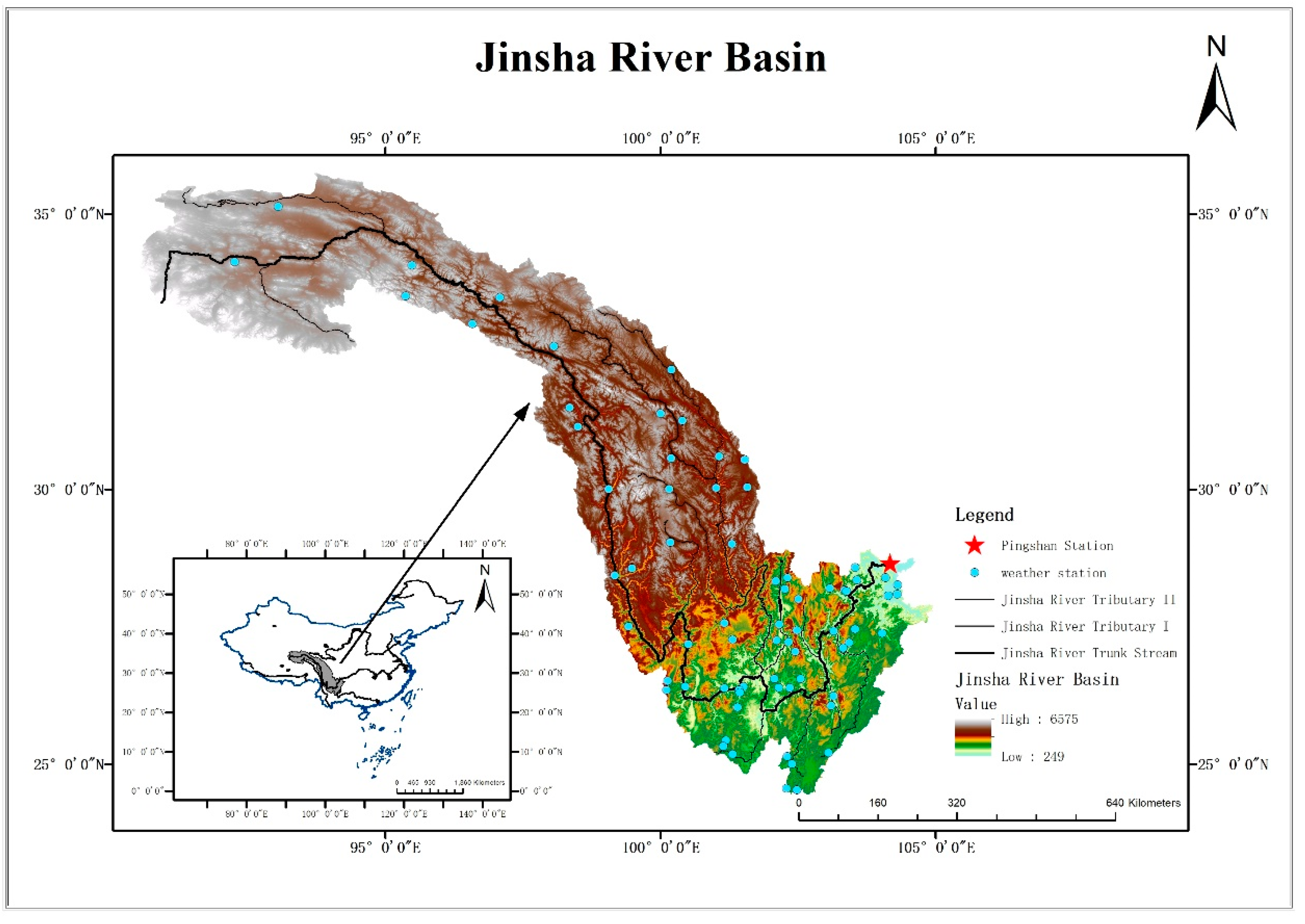
2.1. Study Area and Data Used
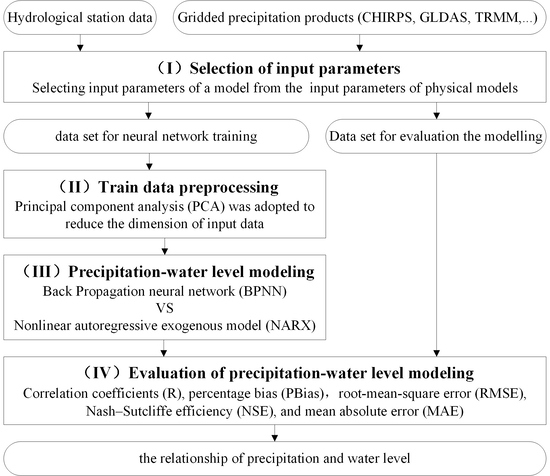
The Jinsha River Basin was taken as the research area. The Jinsha River (24.46°E–35.76°E, 90.535°N–104.936°N, as shown in Figure 1) is located in the upper reaches of the Yangtze River, accounting for 77% of the total length of the upper reaches. The Yangtze River is one of the largest and most important rivers in China. The origin of the Jinsha River is in the main peak of Tanggula Mountain in Qinghai Province. The Jinsha River flows through Qinghai, Tibet, Sichuan, and Yunnan provinces in Western China. The main stream of the Jinsha River has a total length of 2308 kilometers and a drainage area of about 340,000 square kilometers. The topography of the Jinsha River Basin is complex, the elevation fluctuation is obvious [27], the maximum height difference is 3300 m, the annual average precipitation of the Jinsha River Basin is about 710 mm, the annual average precipitation of downstream is about 900–1300 mm, and the annual average precipitation of middle and upstream is about 600–800 mm. The precipitation decreases gradually from southeast to northwest of the basin. Due to the wide area of the Jinsha River Basin, there are obvious differences between precipitation distribution and climate change. The complex geographical conditions also cause uneven distribution of meteorological and hydrological stations in the basin, which leads to the lack of observation. Figure 1 shows the selected Pingshan station in the lower reaches of the Jinsha River, the hydrological situation of the Jinsha River, the topography of the Jinsha River Basin, and the sparse meteorological observation stations in the Jinsha River Basin.
The gauge station selected for the study was the Pingshan hydrological station, which is the core-control hydrological station in the lower reaches of the Jinsha River Basin. The data set of 2006–2009 was selected because there was a dam on the site which had not been completed yet. Considering that the data set of this part of time may not be affected by the upstream dam, the data were from Yangtze River Hydrological Bureau. The span of the data was from 2006 to 2009, the time granularity of the data was 1 day, and the content of the data was the average daily water level. The grid precipitation products used in this paper are CHIRPS, GLDAS-2, and TRMM-V7. All the data are listed as Table 1.
Three different resolution grid precipitation products were used for this paper. One was CHIRPS from http://chg.geog.ucsb.edu/data/chirps/ in a grid format with a spatial resolution of 0.05° × 0.05° and a temporal resolution of 1 day. The second one was the GLDAS-2 from https://ldas.gsfc.nasa.gov/gldas/ with 0.25° × 0.25° spatial and 1 day temporal resolutions. The last one was TRMM-V7 from https://pmm.nasa.gov/data-access/downloads/TRMM with 0.25°× 0.25° spatial and 1 day temporal resolutions.
The CHIRPS data formed a quasi-global precipitation dataset, which was from 1981 to 2014. Spanning 50°S–50°N (and all longitudes) [28], CHIRPS is a fusion of satellite images and data from rain-gauge stations, which is widely used for hydrology modeling, where there are sparse in situ rainfall stations. Bai et al. (2018) compared CHIRPS data with 2480 rainfall stations in China. Although the accuracy of CHIRPS data is not ideal when compared with a single rainfall station, it performs well at the watershed scale [29].
The GLDAS data uses multiple land surface models to integrate satellite and ground-based observational data [30]. GLDAS products include weather forcing data, land surface states data, and flux data. The GLDAS-2 product uses the “Global Meteorological Forcing Dataset” from Princeton University [31] to create more climatologically consistency than GLDAS-1. Wang et al. (2016) evaluated the accuracy of GLDAS-1 and GLDAS-2 monthly data in major watersheds of China, and the results showed that GLDAS-2 data had better spatial and temporal accuracy than GLDAS-1 data for precipitation, temperature, and runoff [32].
The TRMM is a joint mission between NASA and the Japan Aerospace Exploration (JAXA) Agency to study rainfall for weather and climate research, and the dataset of TRMM is intended to provide a relative precise estimation of quasi-global precipitation [20]. TRMM-V6 and V7 data both show a good agreement in the tropics, especially for moderate and heavy rain days. For heavy rain, the rainfall estimates of V6 are higher than V7 in the whole year [33]. For the Jinsha River Basin in the upper reaches of the Yangtze River, TRMM-V6 and TRMM-V7 can better reflect the annual change trend of precipitation in the study basin, among which the estimated results of TRMM-V7 are closer to the measured precipitation results, the estimated results of TRMM-V7 in 2007, 2008, and 2009 are very close to the measured precipitation, and the overall results of V6 are about 100 mm lower. The estimated result of TRMM-RTV7 is about 300 mm higher overall [24]. Thus, we chose the TRMM-V7 dataset for this paper.
In order to ensure the consistency of data sampling, the study used weather forcing data of GLDAS-2 as a grid input in combination with the grid precipitation product. Meanwhile, we used the Daily Climate Data Set of China Ground International Exchange Station (V3.0) for the control experiment. This dataset included daily data of air pressure, temperature, precipitation, evaporation, relative humidity, wind direction, wind speed, sunshine hours, and 0 cm ground temperature elements of 166 stations in China since January 1951 to the near present, which was provided by the National Meteorological Information Center of China (http://data.cma.cn/data/cdcdetail/dataCode/SURF_CLI_CHN_MUL_DAY_V3.0.html).

2.2. Methodology

In order to solve the problems of data-driven modeling, such as model selection, input variable selection, and the impact of different data sources, the method developed in this paper was divided into four parts (I, II, III, IV), as shown below (Figure 2).
  • (I) Selection of input parameters: This part determined the inputs of the used models. Considering the physical model, the input variables of the neural network were selected by referring to the physical process of the hydrological model in part I.
  • (II) Train data preprocessing: This part prepared training data for the neural network models. To improve the performance of the neural network model and avoid the over-fitting of models, the unnecessary information and some noise were removed by the principal component analysis (PCA) dimensionality reduction in order to speed up the convergence of the model in part II.
  • (III) Precipitation–water level modeling: This part compared the modeling methods. As for model fitting, we chose a BP neural network to build the relationship between precipitation and water level; meanwhile, a NARX time series network was also chosen to build the relationship between precipitation and water level in part III.
  • (IV) Evaluation of precipitation–water level modeling: This part chose correlation coefficients (R), percentage bias (PBias), root-mean-square error (RMSE), Nash–Sutcliffe efficiency (NSE), and mean absolute error (MAE) as the criteria for the evaluation of precipitation–water level modeling.

2.2.1. Selection of Input Parameters

Some existing studies use a data-driven method to construct the relationship of precipitation and water level. The influence of precipitation on water level is usually only considered when building the model, but the natural water cycle is a complex physical process. Soil moisture, vegetation transpiration, surface confluence, and other parameters will also affect water level and runoff. Based on regression analysis, Jun Du et al. proved that the effects of annual precipitation and forest cover on runoff change were 69.8% and 17.3% [34]. Existing data-driven models cannot explain the physical phenomena of water level change; therefore, the input parameters of the neural network model are screened by referring to the existing hydrological model. In this study, we investigated existing hydrological models and selected variables by referring to the inputs of hydrological models.
Many hydrological models include a surface module, snow module, meteorological driving module, frozen soil module for calculating the effect of the freezing–thawing process on heat flux and humidity, lake and wetland module for calculating the water–heat balance of lakes and wetlands, carbon cycle module, and confluence algorithm for connecting the grids with river channels [35]. Due to the difficulty of data acquisition and computational complexity, the modules generally considered in estimating runoff yield and confluence using the hydrological model are the surface module, meteorological driving module, and confluence module; that is, the digital elevation model (DEM) grid data, meteorological data, soil data, and vegetation parameters data of the study area.
Hornik proved that the neural network algorithm is a universal approximator [36]. With only one hidden layer containing enough neurons, the multi-layer feedforward neural network can approximate any continuous function with arbitrary precision. According to the characteristics of the neural network algorithm, the input parameters with constant values can be removed because constants can be merged in a function of any kind. The final input parameters of the model are the meteorological data, soil data, and evapotranspiration parameters of the Jinsha River Basin.

2.2.2. Train Data Preprocessing

In order to solve the problem of the high dimensionality of input parameters caused by remote sensing data input, principal component analysis (PCA) was adopted to reduce the dimensions of input data in our study. The purpose of dimension reduction is to use low-dimensional data to retain as much information as possible from the original high-dimensional data; that is, to project the original high-dimensional spatial data to the target low-dimensional subspace through linear mapping to achieve the effect of dimension reduction. PCA is computed as follows, using the covariance method.
  • Here is a sample set D:
    D = { x 1 , x 2 , , x m } ,
  • Decentralize all samples:
    x i x i 1 m i = 1 m x i ,
  • Compute the covariance matrix of samples: XXT;
  • Eigenvalue decomposition of covariance matrix XXT;
  • Extract the d largest characteristic value eigenvalues:
    w 1 , w 2 , , w d ,
  • Output the projection matrix after dimension reduction:
    W = { w 1 , w 2 , , w d } ,
After the dimensionality reduction of input data, it was inevitable to discard some information from the original data, but at the same time, we could remove some noise that deviated from the sample center too much. For the neural network model to be used in the study, too many dimensions of input samples could easily lead to the over-fitting of the model and bad generalization, thus leading to poor prediction results of the model.

2.2.3. Precipitation–Water Level Modeling

In order to better simulate the delayed effect of the water level change process, modeling the relationship between precipitation and water level needs to consider time variation. A nonlinear autoregressive exogenous model (NARX) was selected in this paper. To show the effect of the time series network model, this paper used the BP neural network model as a comparison.

Back Propagation Neural Network Model

Back propagation neural network (BPNN) is a feedforward neural network trained by the error back propagation (BP) algorithm [37]. It is the most widely used network in the field of prediction and modeling. The key to the BP neural network is that signals propagate forward and errors propagate backward.
The BP algorithm is based on gradient descent strategy. The goal of the gradient descent algorithm is to minimize the cumulative error on the training set; the gradient vector of the loss function is obtained by the chain derivation rule and then the error value of the output layer node is obtained. By using the error value of the output layer node as the reverse input, the connection weights and thresholds of the neural network were updated. We looped the update process until the termination condition of network training (maximum training times, minimum error, maximum iteration times, etc.) was reached.

Nonlinear Autoregressive Exogenous Model

The nonlinear autoregressive exogenous model (NARX), developed by Tsungnan Lin [38], is a recurrent network that has exogenous inputs. That means that the output of the model depends both on past values of the previous output and current and past values of independent variable series.
Compared with the BP neural network, the NARX network correlates the past observed (or predicted values) with the current target values through a time delay variable (d), which can more accurately model the observation variables associated with the time series. The function of the NARX time series network model is expressed as follows, where y ( t ) is the output target value on the t day, x ( t ) is the input variable value on day t , and d is the time delay days. The delay time is often determined by multiple prediction experiments; here, we got the best prediction result by repeated experiments, which are recorded in Section 3.2.1. If the delay time was too long or too short, the NARX model was under-fitted or oscillate.
y ( t ) = f ( x ( t 1 ) , , x ( t d ) , y ( t 1 ) , , y ( t d ) )
NARX can be inputted externally through observed data, i.e., parallel mode. It can also be inputted through the target predicted value; i.e., the serial mode. The parallel mode had higher prediction accuracy because it used the exact value of observed data. As the ground stations can obtain the accurate daily water level, the parallel model was adopted in this study. Usually, the hydrological process is a slow cumulative process, and water level changes are usually associated with past water level, so the NARX time series network model can better explain the process of water level changes, and more accurate results of water level changes can be obtained theoretically.

2.2.4. Evaluation of Precipitation–Water Level Modeling

The main criteria for evaluating the efficacy of prediction models are the correlation coefficients (R), percentage bias (PBias), root-mean-square error (RMSE), Nash–Sutcliffe efficiency (NSE), and mean absolute error (MAE), which is commonly used to assess the quality of hydrological models. The validation coefficients are expressed as follows:
R = i = 1 n [ ( O i O ¯ ) ( P i P ¯ ) ] [ ( i = 1 n ( O i O ¯ ) 2 ) ( i = 1 n ( P i P ¯ ) 2 ) ] ,
P B i a s = i = 1 n ( P i O i ) i = 1 n O i × 100
R M S E = 1 n i = 1 n ( P i O i ) 2
N S E = [ 1 i = 1 n ( O i P i ) 2 i = 1 n ( O i O ¯ ) 2 ] × 100 %
M A E = 1 n i = 1 n | O i P i |
where n is the number of predictions, O i is the observed value of water level (i.e., the measured value), P i is the predicted value of water level output from the model, O ¯ is the average value of water level observation, and P ¯ is the average water level prediction value. Through comparative experiments, the model accuracy of different inputs and different networks was evaluated.

3. Results and Discussion

In order to study the possible influencing factors in the precipitation–water level model, we carried out several groups of comparative experiments. Considering the instantaneousness of water level observation, we used an n-7 sliding window and divided the data into 1543 groups of 8 days (the first 7 days of each group and the eighth day of training) as the prediction. The size of the sliding window came from many attempts during parameter adjustment. Through the results of these groups of comparative experiments, we can give some guidance as to the construction of the relationship of precipitation–water level.
We divided the input of the neural network model into a precipitation part, which directly affected the water level change, and an extra meteorological input (EMI) part, which had an indirect effect on the water level change. The additional meteorological input data included soil moisture data, temperature data, wind speed data, and evapotranspiration data. We used the precipitation observation data of in situ station data, CHIRPS precipitation products, GLDAS-2 precipitation products, and TRMM-V7 precipitation products as inputs, and the meteorological inputs used the assimilation data in GLDAS-2. At the same time, in order to verify the modeling results of surface precipitation modeling, we used a full station input for a contrast experiment (the last group). To explore the influence of different networks on the modeling results of the precipitation–water level model, each group of inputs used different network models for water level simulation. Furthermore, we resampled the grid precipitation products into different resolutions to explore the impact of different resolutions on the modeling results. Table 2 shows the accuracy of all type of models mentioned above.

3.1. Comparison of Different Grid Precipitation Products with Respect to the Observed Data

In order to preliminarily verify the availability of grid precipitation products, this paper makes a simple evaluation regarding the accuracy of grid precipitation products. Figure 3 shows the scatter plots of the areal precipitation time series of CHIRPS, GLDAS-2, and TRMM-V7 against the rainfall data of the in situ station from 2006 to 2009. The CHIRPS precipitation product had a correlation of 0.606 with the in situ station data (Figure 3a) and the GLDAS-2 precipitation product had a correlation of 0.733 (Figure 3b), whereas the TRMM-V7 product had a correlation of 0.645 (Figure 3c).
Table 3 shows the comparison of the accuracy of daily precipitation mean values of three grid precipitation products (CHIRPS, GLDAS-2, TRMM-V7) and ground precipitation stations. It can be seen from the table that GLDAS-2 data had the highest correlation, but the percentage bias of data was also the largest. Generally, grid precipitation products tended to underestimate the extreme value of rainfall, but the average value was relatively reliable.

3.2. Performance of the BP Neural Network Model and NARX Network Model for Water Level Modeling

3.2.1. Parameter Optimization of Neural Network

Although multilayer feedforward neural networks can approximate arbitrary continuous functions, it is usually impossible to tell the absolute number of hidden layers of networks and the number of neurons in hidden layers, but there are some general parameter setting rules summarized by previous studies. Generally speaking, due to the structure limitations of the training data and network model, the simulation effect of the feedforward neural network model with two hidden layers is usually better than that with only one hidden layer [39]. Here, we used different kinds and resolutions of grid precipitation products, and the number of input nodes in each group of neural networks was determined by the results of the principal components analysis (PCA) dimensionality reduction processing. The node number of the first hidden layer was N 1 = D i + 1 + 1 , where D i . is the dimension of the independent input variable; the second one was N 2 = N 1 + 3 . Moreover, the transfer functions of the network were of Tansig types. The selection of parameters used in this paper was a relatively optimal solution obtained by multiple parameter adjustment, and all the training parameters used are shown in Table 4.
In order to get better modelling results, we made some adjustments to the parameters of the neural network. We optimized the network parameters by the method of artificially adjusting parameters and we performed preliminary experiments to determine the network parameters and further adjusted them in the actual experiment. Table 5 shows the result of the cross-correlation function between rainfall gauge data and the water level of Pingshan station. We found that when the time delay was 6, the correlation between the rainfall series and water level series reached a maximum of 0.7559. Based on the results of cross-correlation function (CCF), we gradually adjusted the time delay parameter in the NARX network model. After many experiments, we found that when the time lag was 5 days, the performance of the NARX model reached the optimal value.

3.2.2. Modeling Results of BP Neural Network Model and NARX Network

The BP neural network is the most popular network in the field of prediction, but its performance in precipitation–water level modeling is not as good as the NARX network, as shown in Figure 4. Figure 4 shows the line plots of observed data and simulated water level using different neural network models with the input of GLDAS-2+EMI: The red line is the modeling result of using the BPNN and the blue line is the modeling result of using the NARX network. From the graph, we can see that the result of water level modeling using the NARX model was closer to the observed value. Additionally, as shown in Table 2, we found that the R² value of the water level modeling using the BP neural network model was 0.93 to 0.94 and the R² value of modeling results using the NARX model was 0.97 to 0.98. Although the four sets of experiments used different neural network model input variables, the results of using the NARX model for water level modeling were better in each group of experiments.
Table 6 shows the average value of modeling results using two different neural networks, and from Table 6 we can get more precise results regarding the use of the BP neural network model and NARX network model, from which we can obviously see that the NARX model performed better than the BP model in the four performance evaluation criteria. Although the correlation coefficients of the BP model and NARX model were more than 0.95, the average correlation coefficient of the NARX prediction results was 2% higher than that of the BP model. However, the average percentage bias of the NARX model was 0.00032%, while the BP neural network model was 0.00041%. As for RMSE, the mean RMSE of the BP model was 1.072 m, but that of NARX was 0.606 m, and the Nash–Sutcliffe efficiency of the two models was higher than 50%; thus, both kinds of neural network model were reliable, but the NARX model was more reliable, as the NSE of it was over 97%.
All criteria for the performance evaluation show that the NARX model performed better than the BPNN model in short-term water level modeling, which was consistent with our expectations, but the percentage bias of the BP neural network was smaller on the whole. As the NARX model used past rainfall input values and water level observations, considering the delayed effect of hydrological processes, the fitting results of the NARX network could get closer to the complex hydrological processes in the real world. Using NARX network for model construction can also better explain the relationship between rainfall and water level, and it can be seen from Figure 4 that for the BPNN, the NARX network produced less model oscillation and lower probability of extreme value.

3.3. Comparison of Modeling Results using Grid Products and Station Data

In order to verify the availability of grid products in precipitation–water level modeling, we compared the modeling results of grid products with the modeling results of ground stations. Table 7 shows the impact of different types of rainfall data input on water level modeling results: The average correlation coefficients of grid data modeling and station data using the NARX network were both 0.988,and, using GLDAS-2 0.25° with EMI as an input showed the best result, the RSME of which was 0.561 m and the Nash efficiency coefficient was 97.858%, while the Nash efficiency coefficient of using station data was 97.560%. Combined with Table 2, we found that the percentage bias of station data was relatively small, which was −0.00060%.
From Figure 5, we can see more intuitively that the accuracy of modeling results with grid precipitation data was little different from that with station data. In addition, although using GLDAS-2 0.25° with EMI as an input showed the smallest RSME and the highest correlation coefficient with observed data, the average percentage bias of GLDAS-2 was larger than the other group. It can be seen from the above results that it was feasible to use grid rainfall products as the solution of sparse area of stations. Because the grid data integrated the results of the satellite data and the ground station data, it was more reliable than the conventional spatial interpolation results of ground station data. In this experiment, the prediction result using grid data input was slightly better than that using only ground station.

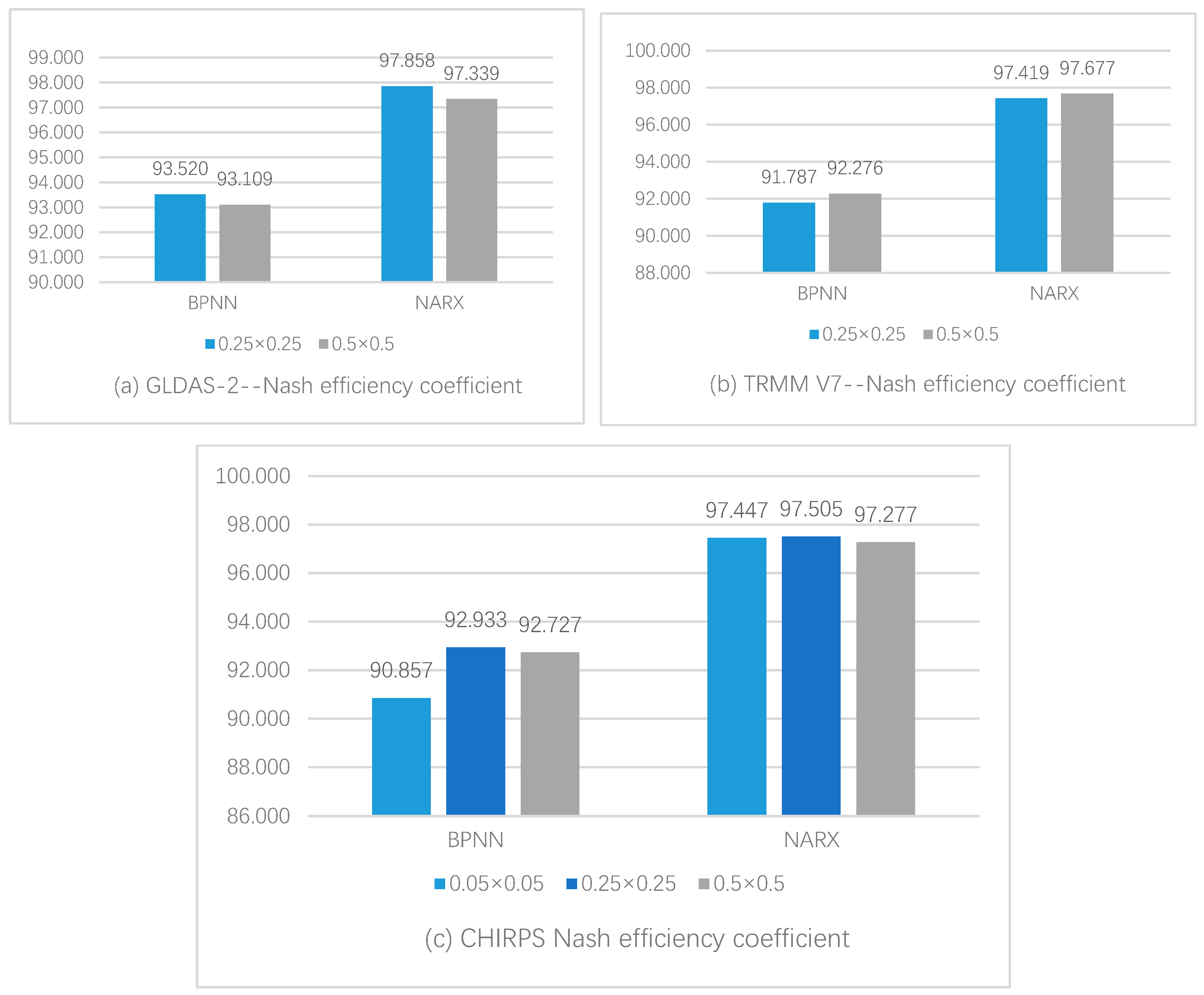
3.3.1. Influence of using Different Precipitation Products

In order to verify the influence of different grid precipitation products on the model construction, we resampled the three products of CHIRPS, GLDAS-2, and TRMM-V7 to 0.25° and constructed the model. The final experimental results are shown in Table 8. The Nash efficiency coefficients of using CHIRPS, GLDAS-2, and TRMM-V7 data based on the BPNN model were 93%, 91%, and 92%, and those of the NARX model were all above 97%.
Figure 6 shows the accuracy histogram of three different products; we can find that the GLDAS –2 data modeling results were the best by comprehensive comparison. The R of using GLDAS-2 with the NARX network was 0.989, the RSME was 0.561 m, and the Nash efficiency coefficient was 97.858%. However, modeling with TRMM-V7 and CHIRPS data showed less percentile deviation. For the Jinsha River Basin, GLDAS-2 data was the best rainfall input among the above three kinds of rainfall products, but the performance gap of the three kinds of grid precipitation products was not large, in which the absolute deviation of CHIRPS group was the smallest, which may have been due to the better performance of CHIRPS data on the extreme value of rainfall estimation.

3.3.2. Influence of using Different Resolution Products

In order to explore the influence of grid product resolution on model building, we resampled each grid product to a different resolution: GLDAS-2 and TRMM data were resampled to 0.5° (the original resolution was 0.25°) and CHIRPS data were resampled to 0.25 and 0.5 degrees (the original resolution was 0.05°), as shown in Figure 7. The Nash efficiency coefficients of using BPNN with CHIRPS input for 0.05°, 0.25°, and 0.5° were 90.857%, 92.933%, and 92.727%, while those using the NARX network were 97.447%, 97.505%, and 97.277%. From Figure 7, we can see that the grid product input with different resolutions had little influence on the modeling results. For the CHIRPS and TRMM data, the prediction accuracy of products with higher resolution was slightly reduced, but for GLDAS-2 data, the high-resolution input modeling results were slightly better. For the input of different resolutions of the same precipitation product, the short-term water level prediction accuracy using spatial resolutions of 0.25 °× 0.25 ° and 0.5 °× 0.5 ° had little difference and the model prediction result of the high spatial resolution grid data input of chirps did not significantly improve, which may have been due to the model over-fitting problem caused by the high input dimension. For model training, using 0.5 ° × 0.5 ° spatial resolution data for input can significantly improve the processing speed of the model, so the use of low and medium resolution data can be considered in the process of model training.
In total, when choosing the BP neural network model as the fitting model, using in-site stations, CHIRPS and GLDAS-2 data as input data sources did not have an obvious influence on the prediction results, and grid precipitation products could get similar results to rain-gauge station inputs. When selecting the NARX network as a fitting model, the results of using the GLDAS-2 precipitation product as an input were generally better than those of using rain-gauge station inputs and CHIRPS data. There was little difference between the accuracy of simulation results by using grid precipitation products and that by using ground stations. The results of using ground stations to build the model were almost the same as using grid precipitation products. When GLDAS-2 data were used as a model input, the result of water level modeling was slightly better than that of the ground station. However, the percentage deviation between the two models using the in-site station as an input was better than using precipitation products, which was due to the grid precipitation products tending to underestimate high rainfall values [40].

4. Conclusions

Precipitation–water level modeling usually lacks a clear model-building mechanism. In this study, we showed a specific data-driven process for grid precipitation–water level modeling and evaluated the accuracy of the model. The different data were used as input variables for the two different neural network models. The results of this study lead to the following conclusions:
  • Compared with the BP neural network, the NARX time series network can significantly improve the accuracy of water level modeling, which is related to the NARX network, considering the time lag effect.
  • Compared with the ground station, the grid data can get similar results in general. The GLDAS 2 data are better than the ground station in water level modeling. Therefore, in an area where the water level station is missing, the surface rainfall data can be used as an available alternative of ground battle points for water level modeling experiments.
  • Under the same resolution, the water level modeling results with different data sources are similar, although the GLDAS 2 results are slightly better. Using the same data source, the experimental results of water level modeling with different resolutions of surface rainfall data have little difference, so it is of little significance to pursue high-resolution surface rainfall products in the construction of a precipitation–water level model.
  • In this paper, by putting forward a method for building a precipitation–water level model, the influencing factors of each part of the water level model are discussed, which has certain guiding significance for future research into water level modeling.
At present, our research can only predict the short-term water level and does not consider the influence of distance effect in the basin on the time delay of rainfall water level process. In the future, we will continue to consider the use of the machine learning method to predict the medium and long-term water level and divide the distance according to the spatial correlation factors in the basin.

Author Contributions

Conceptualization: Z.C., X.L., and N.C.; methodology: Z.C., X.L., and N.C.; formal analysis: Z.C., X.L., C.X., and N.C.; writing—original draft preparation: Z.C., X.L., and C.X.; writing—review and editing: X.L., Z.C., and C.X.; supervision: N.C. and Z.C.; funding acquisition: N.C. and Z.C. All authors have read and agreed to the published version of the manuscript.

Funding

This work is supported by the National Nature Science Foundation of China program (nos. 41971351, 41771422, 41890822).

Acknowledgments

The water level data used during the study were provided by the ChangJiang Water Resources Commission of the Ministry of Water Resources (http://www.cjw.gov.cn/). The meteorological data used during the study were provided by the National Meteorological Information Center, China (http://data.cma.cn/data/cdcdetail/dataCode/A.0012.0001.html). The CHIRPS data set was provided by the Climate Hazards Group(https://chg.geog.ucsb.edu/data/chirps). The TRMM data set was provided by the American Meteorological Society Data Archiving (https://pmm.nasa.gov/data-access/downloads/TRMM). The GLDAS-2 data was provided by NASA (https://ldas.gsfc.nasa.gov/gldas/).

Conflicts of Interest

The authors declare no conflict of interest.

References

  1. Chen, N.; Xiong, C.; Du, W.; Wang, C.; Lin, X.; Chen, Z. An Improved Genetic Algorithm Coupling a Back-Propagation Neural Network Model (IGA-BPNN) for Water-Level Predictions. Water 2019, 11, 1795. [Google Scholar] [CrossRef] [Green Version]
  2. Liang, X.; Lettenmaier, D.P.; Wood, E.F.; Burges, S.J. A simple hydrologically based model of land surface water and energy fluxes for general circulation models. J. Geophys. Res. Atmos. 1994, 99, 14415–14428. [Google Scholar] [CrossRef]
  3. Arnold, J.G.; Moriasi, D.N.; Gassman, P.W.; Abbaspour, K.C.; White, M.J.; Srinivasan, R.; Santhi, C.; Harmel, R.; Van Griensven, A.; Van Liew, M.W. SWAT: Model use, calibration, and validation. Trans. ASABE 2012, 55, 1491–1508. [Google Scholar] [CrossRef]
  4. Ren-Jun, Z. The Xinanjiang model applied in China. J. Hydrol. 1992, 135, 371–381. [Google Scholar] [CrossRef]
  5. Tong, K.; Su, F.; Yang, D.; Hao, Z. Evaluation of satellite precipitation retrievals and their potential utilities in hydrologic modeling over the Tibetan Plateau. J. Hydrol. 2014, 519, 423–437. [Google Scholar] [CrossRef]
  6. Hao, Z.-C.; Tong, K.; Liu, X.-L.; Zhang, L.-L. Capability of TMPA products to simulate streamflow in upper Yellow and Yangtze River basins on Tibetan Plateau. Water Sci. Eng. 2014, 7, 237–249. [Google Scholar]
  7. Liu, X.; Yang, T.; Hsu, K.; Liu, C.; Sorooshian, S. Evaluating the streamflow simulation capability of PERSIANN-CDR daily rainfall products in two river basins on the Tibetan Plateau. Hydrol. Earth Syst. Sci. (Online) 2017, 21. [Google Scholar] [CrossRef] [Green Version]
  8. Dhar, V. Data science and prediction. Commun. ACM 2013, 56, 64–73. [Google Scholar] [CrossRef]
  9. Khan, M.; Hasan, F.; Panwar, S.; Chakrapani, G. Neural network model for discharge and water-level prediction for Ramganga River catchment of Ganga Basin, India. Hydrol. Sci. J. 2016, 61, 2084–2095. [Google Scholar] [CrossRef] [Green Version]
  10. Leahy, P.; Kiely, G.; Corcoran, G. Structural optimisation and input selection of an artificial neural network for river level prediction. J. Hydrol. 2008, 355, 192–201. [Google Scholar] [CrossRef]
  11. Maier, H.R.; Dandy, G.C. Neural networks for the prediction and forecasting of water resources variables: A review of modelling issues and applications. Environ. Model. Softw. 2000, 15, 101–124. [Google Scholar] [CrossRef]
  12. Piasecki, A.; Jurasz, J.; Skowron, R. Forecasting surface water level fluctuations of lake Serwy (Northeastern Poland) by artificial neural networks and multiple linear regression. J. Environ. Eng. Landsc. Manag. 2017, 25, 379–388. [Google Scholar] [CrossRef] [Green Version]
  13. Zhong, C.; Jiang, Z.; Chu, X.; Guo, T.; Wen, Q. Water level forecasting using a hybrid algorithm of artificial neural networks and local Kalman filtering. Proc. Inst. Mech. Eng. Part M J. Eng. Marit. Environ. 2019, 233, 174–185. [Google Scholar] [CrossRef]
  14. Manandhar, S.; Dev, S.; Lee, Y.H.; Meng, Y.S.; Winkler, S. A Data-Driven Approach for Accurate Rainfall Prediction. IEEE Trans. Geosci. Remote Sens. 2019, 57, 9323–9331. [Google Scholar] [CrossRef] [Green Version]
  15. Sahoo, A.; Samantaray, S.; Bankuru, S.; Ghose, D.K. Prediction of Flood Using Adaptive Neuro-Fuzzy Inference Systems: A Case Study. In Smart Intelligent Computing and Applications; Springer: Singapore, 2020; pp. 733–739. [Google Scholar]
  16. Samantaray, S.; Sahoo, A. Appraisal of runoff through BPNN, RNN, and RBFN in Tentulikhunti Watershed: A case study. In Frontiers in Intelligent Computing: Theory and Applications; Springer: Singapore, 2020; pp. 258–267. [Google Scholar]
  17. Samantaray, S.; Sahoo, A. Estimation of runoff through BPNN and SVM in Agalpur Watershed. In Frontiers in Intelligent Computing: Theory and Applications; Springer: Singapore, 2020; pp. 268–275. [Google Scholar]
  18. Garcia, F.C.C.; Retamar, A.E.; Javier, J.C. Development of a predictive model for on-demand remote river level nowcasting: Case study in Cagayan River Basin, Philippines. In Proceedings of the 2016 IEEE Region 10 Conference (TENCON), Singapore, 22–25 November 2016; pp. 3275–3279. [Google Scholar]
  19. Adnan, R.; Ruslan, F.A.; Samad, A.M.; Zain, Z.M. Flood water level modelling and prediction using artificial neural network: Case study of Sungai Batu Pahat in Johor. In Proceedings of the 2012 IEEE Control and System Graduate Research Colloquium, Shah Alam, Selangor, Malaysia, 16–17 July 2012; pp. 22–25. [Google Scholar]
  20. Huffman, G.J.; Bolvin, D.T.; Nelkin, E.J.; Wolff, D.B.; Adler, R.F.; Gu, G.; Hong, Y.; Bowman, K.P.; Stocker, E.F. The TRMM multisatellite precipitation analysis (TMPA): Quasi-global, multiyear, combined-sensor precipitation estimates at fine scales. J. Hydrometeorol. 2007, 8, 38–55. [Google Scholar] [CrossRef]
  21. Nanda, T.; Sahoo, B.; Beria, H.; Chatterjee, C. A wavelet-based non-linear autoregressive with exogenous inputs (WNARX) dynamic neural network model for real-time flood forecasting using satellite-based rainfall products. J. Hydrol. 2016, 539, 57–73. [Google Scholar] [CrossRef]
  22. Chen, P.-A.; Chang, L.-C.; Chang, F.-J. Reinforced recurrent neural networks for multi-step-ahead flood forecasts. J. Hydrol. 2013, 497, 71–79. [Google Scholar] [CrossRef]
  23. Nourani, V.; Baghanam, A.H.; Adamowski, J.; Gebremichael, M. Using self-organizing maps and wavelet transforms for space–time pre-processing of satellite precipitation and runoff data in neural network based rainfall–runoff modeling. J. Hydrol. 2013, 476, 228–243. [Google Scholar] [CrossRef]
  24. Huang, Y. Application of TRMM Precipitation in VIC Hydrological Model for Streamflow Simulations in the Upstream of Yangtze River. Master’s Thesis, Nanjing Forestry University, Nanjing, China, 2017. [Google Scholar]
  25. Guo, D.; Wang, H.; Zhang, X.; Liu, G. Evaluation and Analysis of Grid Precipitation Fusion Products in Jinsha River Basin Based on China Meteorological Assimilation Datasets for the SWAT Model. Water 2019, 11, 253. [Google Scholar] [CrossRef] [Green Version]
  26. Tuo, Y.; Duan, Z.; Disse, M.; Chiogna, G. Evaluation of precipitation input for SWAT modeling in Alpine catchment: A case study in the Adige river basin (Italy). Sci. Total Environ. 2016, 573, 66–82. [Google Scholar] [CrossRef] [Green Version]
  27. Zhang, Q.; Xu, C.-Y.; Becker, S.; Jiang, T. Sediment and runoff changes in the Yangtze River basin during past 50 years. J. Hydrol. 2006, 331, 511–523. [Google Scholar] [CrossRef]
  28. Funk, C.; Peterson, P.; Landsfeld, M.; Pedreros, D.; Verdin, J.; Shukla, S.; Husak, G.; Rowland, J.; Harrison, L.; Hoell, A. The climate hazards infrared precipitation with stations—A new environmental record for monitoring extremes. Sci. Data 2015, 2, 150066. [Google Scholar] [CrossRef] [Green Version]
  29. Bai, L.; Shi, C.; Li, L.; Yang, Y.; Wu, J. Accuracy of CHIRPS satellite-rainfall products over mainland China. Remote Sens. 2018, 10, 362. [Google Scholar] [CrossRef] [Green Version]
  30. Rodell, M.; Houser, P.; Jambor, U.; Gottschalck, J.; Mitchell, K.; Meng, C.-J.; Arsenault, K.; Cosgrove, B.; Radakovich, J.; Bosilovich, M. The global land data assimilation system. Bull. Am. Meteorol. Soc. 2004, 85, 381–394. [Google Scholar] [CrossRef] [Green Version]
  31. Sheffield, J.; Goteti, G.; Wood, E.F. Development of a 50-year high-resolution global dataset of meteorological forcings for land surface modeling. J. Clim. 2006, 19, 3088–3111. [Google Scholar] [CrossRef] [Green Version]
  32. Wang, W.; Cui, W.; Wang, X.; Chen, X. Evaluation of GLDAS-1 and GLDAS-2 Forcing Data and Noah Model Simulations over China at the Monthly Scale. J. Hydrometeorol. 2016, 17, 2815–2833. [Google Scholar] [CrossRef]
  33. Liu, Z. Comparison of versions 6 and 7 3-hourly TRMM multi-satellite precipitation analysis (TMPA) research products. Atmos. Res. 2015, 163, 91–101. [Google Scholar] [CrossRef] [Green Version]
  34. Du, J.; Shi, C.-X. Modeling and analysis of effects of precipitation and vegetation coverage on runoff and sediment yield in Jinsha River Basin. Water Sci. Eng. 2013, 6, 44–58. [Google Scholar]
  35. Hamman, J.J.; Nijssen, B.; Bohn, T.J.; Gergel, D.R.; Mao, Y. The Variable Infiltration Capacity model version 5 (VIC-5): Infrastructure improvements for new applications and reproducibility. Geosci. Model Dev. 2018, 11, 3481–3496. [Google Scholar] [CrossRef] [Green Version]
  36. Hornik, K.; Stinchcombe, M.; White, H. Multilayer feedforward networks are universal approximators. Neural Netw. 1989, 2, 359–366. [Google Scholar] [CrossRef]
  37. Rumelhart, D.E.; Hinton, G.E.; Williams, R.J. Learning representations by back-propagating errors. In Neurocomputing: Foundations of Research; James, A.A., Edward, R., Eds.; MIT Press: Cambridge, MA, USA, 1988; pp. 696–699. [Google Scholar]
  38. Lin, T.; Horne, B.G.; Tino, P.; Giles, C.L. Learning long-term dependencies in NARX recurrent neural networks. IEEE Trans. Neural Netw. 1996, 7, 1329–1338. [Google Scholar]
  39. Thomas, A.J.; Petridis, M.; Walters, S.D.; Gheytassi, S.M.; Morgan, R.E. Two hidden layers are usually better than one. In Proceedings of the International Conference on Engineering Applications of Neural Networks, Athens, Greece, 25–27 August 2017; pp. 279–290. [Google Scholar]
  40. Paredes-Trejo, F.J.; Barbosa, H.; Kumar, T.L. Validating CHIRPS-based satellite precipitation estimates in Northeast Brazil. J. Arid Environ. 2017, 139, 26–40. [Google Scholar] [CrossRef]
Figure 1. The Jinsha River Basin.
Remotesensing 12 01096 g001
Figure 2. Main processes of modeling the relationship of precipitation and water level using grid precipitation products with the neural network model.
Remotesensing 12 01096 g002
Figure 3. Accuracy evaluation of grid precipitation data. (a) Daily average precipitation scatter plot of CHIRPS data and station data. (b) Daily average precipitation scatter plot of GLDAS-2 data and station data. (c) Daily average precipitation scatter plot of TRMM-V7 data and station data.
Remotesensing 12 01096 g003
Figure 4. Plots of observed data and water level modeling using different neural network models.
Remotesensing 12 01096 g004
Figure 5. Comparison of modeling results using grid products and station data.3.4. Influence on water level modeling results using different precipitation products and different resolutions.
Remotesensing 12 01096 g005
Figure 6. Comparison of water level modeling for different products.
Remotesensing 12 01096 g006
Figure 7. Comparison of performance of the water level modeling using different resolutions. (a) Nash efficiency coefficient for water level prediction using GLDAS-2 data. (b) Nash efficiency coefficient for water level prediction using TRMM-V7 data. (c) Nash efficiency coefficient for water level prediction using CHIRPS data.
Remotesensing 12 01096 g007
Table 1. Data list of this paper. Climate hazards group infrared precipitation with station data (CHIRPS); global land data assimilation system (GLDAS); tropical rainfall measuring mission (TRMM).
Data NameData TypeTemporal/Spatial ResolutionTime Range
Pingshan Water Level Hydrological station data1 day/-2006/01/01~2009/12/30
CHIRPS Grid data1 day/0.05° × 0.05°
GLDAS-2Grid data1 day/0.25° × 0.25°
TRMM-V7Grid data1 day/0.25° × 0.25°
In situ dataGauge-based data1 day/-
Table 2. Accuracy evaluation of precipitation–water level modeling using different type of models. Extra meteorological input (EMI); spatial resolution (SR); back propagation neural network (BPNN); nonlinear autoregressive exogenous model (NARX); percentage bias (Pbias); root mean square error (RSME); Nash–Sutcliffe efficiency (NSE); mean average error (MAE); correlation coefficients (R).
Network Type BPNNNARX
Data NameSRRPbiasRSMENSEMAERPbiasRSMENSEMAE
GLDAS-2+ EMI0.25°0.967–0.005810.97693.5200.5430.9890.001260.56197.8580.336
0.5°0.9660.002491.00693.1090.5600.987−0.000130.62597.3390.358
TRMM-V7+ EMI0.25°0.9590.007141.09891.7870.5840.987−0.000090.61697.4190.349
0.5°0.9610.002501.06592.2760.5640.9880.001180.58497.6770.342
CHIRPS+ EMI0.05°0.954−0.007921.15990.8570.6320.987−0.002470.61297.4470.353
0.5°0.9650.003251.01992.9330.5640.9880.000070.60597.5050.342
0.25°0.9640.004051.03392.7270.5660.9860.000530.63297.2770.357
Station rainfall data + EMI 0.9630.001801.05392.4500.5620.988−0.000600.59997.5600.335
Use station rainfall input only 0.948–0.003821.24389.4820.6970.9870.003170.61997.3930.359
Table 3. Accuracy evaluation of grid precipitation data.
Accuracy CriteriaRainfall StationCHIRPSGLDAS-2TRMM-V7
R10.6060.73260.645
Pbias (%)0−3.40−17.404.23
Table 4. Model parameters used for the neural network models.
Parameter TypeParameters of Neural Networks
Study parameterLearning rate = 0.01
momentum factor = 0.9
transfer function = 2 1 + e 2 n 1
Structure parameterNumber of input nodes D i : determined by the spatial resolution of input remote sensing data and the result of principal component analysis
Number of the first hidden layer of nodes: N 1 = D i + 1 + 1
Number of the second hidden layer of nodes: N 2 = N 1 + 3
Number of hidden layers = 2
Number of output nodes = 1
Table 5. Cross-correlation function (CCF) between rainfall data and water level.
Time Lag12345678
CCF0.69140.70570.72460.73960.75140.75590.75570.751
Table 6. Average value of modeling results using the two different networks.
RPBiasRSMENSEMAE
BPNN0.9610.000411.07292.1270.586
NARX0.9870.000320.60697.4970.348
Table 7. Modeling results using grid products and station data.
Data NameBPNNNARX
RPbiasRSMENSERPbiasRSMENSE
GLDAS-2+EMI 0.25°0.967−0.00581 0.97693.5200.9890.00126 0.56197.858
average resultsof grid data0.9620.0005741.04992.4850.9880.000340.60097.544
Station Data0.9630.00180 1.05392.4500.988−0.00060 0.59997.560
Table 8. Modeling results using different grid precipitation products.
Data Name BPNNNARX
SRRPbiasRSMENSERPbiasRSMENSE
GLDAS-20.25°0.967−0.00581 0.97693.5200.9890.00126 0.56197.858
TRMM-V70.25°0.9590.00714 1.09891.7870.987−0.00009 0.61697.419
CHIRPS0.25°0.9650.00325 1.01992.9330.9880.000070.60597.505

