Soil Color and Mineralogy Mapping Using Proximal and Remote Sensing in Midwest Brazil

Abstract

Soil color and mineralogy are used as diagnostic criteria to distinguish different soil types. In the literature, 350–2500 nm spectra were successfully used to predict soil color and mineralogy, but these attributes currently are not mapped for most Brazilian soils. In this paper, we provided the first large-extent maps with 30 m resolution of soil color and mineralogy at three depth intervals for 850,000 km² of Midwest Brazil. We obtained soil 350–2500 nm spectra from 1397 sites of the Brazilian Soil Spectral Library at 0–20 cm, 20–60, and 60–100 cm depths. Spectra was used to derive Munsell hue, value, and chroma, and also second derivative spectra of the Kubelka–Munk function, where key spectral bands were identified and their amplitude measured for mineral quantification. Landsat composites of topsoil and vegetation reflectance, together with relief and climate data, were used as covariates to predict Munsell color and Fe–Al oxides, and 1:1 and 2:1 clay minerals of topsoil and subsoil. We used random forest for soil modeling and 10-fold cross-validation. Soil spectra and remote sensing data accurately mapped color and mineralogy at topsoil and subsoil in Midwest Brazil. Hematite showed high prediction accuracy (R² > 0.71), followed by Munsell value and hue. Satellite topsoil reflectance at blue spectral region was the most relevant predictor (25% global importance) for soil color and mineralogy. Our maps were consistent with pedological expert knowledge, legacy soil observations, and legacy soil class map of the study region.

1. Introduction

The color is the most noticeable feature of soil that can be easily determined in field or laboratory [1]. The main factors that influence soil color are the organic matter [2] and mineralogy, especially iron oxides [3]. Soil organic matter causes the darkness of soil by decreasing the Munsell value and chroma [4]. The most frequent pedogenic oxides in soil are hematite (usually associated to goethite), with hues between 10 R and 5 YR, and goethite (without hematite), with hues between 7.5 YR and 2.5 Y [3]. Goethite is common in diverse climates and parent materials, while hematite is abundant in well-drained tropical soils with strong pigmenting effect and is absent in young soils from temperate humid climates [1,5].

In tropical Midwest Brazil, the surface materials are rich in Al, Si, and Fe-bearing minerals, where most of the soils developed from these rocks tend to be low in exchangeable bases and highly weathered [6]. The secondary minerals of these soils are frequently dominated by iron oxides, kaolinite and gibbsite, and 2:1 clay minerals that may resist in the silt and sand fractions [7]. When iron oxides are completely removed (after reduction processes) from soil particles under anaerobic conditions, and if organic matter is negligible, the soil matrix achieves the background color of the minerals resulting in shades of gray [3]. Consequently, color can be used to indicate the presence of minerals and the redoximorphic conditions of the soil [8]. However, in tropical soils, mineralogy cannot be inferred from color alone because hematite has a stronger pigmenting effect than the other soil minerals, including goethite [9].

The iron oxides and soil color are effective pedoenvironmental indicators [3,10]. Various soil classification criteria used by nonscientists, like ethnic groups and farmers across the world, frequently are based on color [11]. Soil management zones, with different productivity potential, can be successfully delineated using bare soil color and topography [12]. Some national [13] and international [14] soil classification systems use the color patterns and mineral contents of soil as diagnostic criteria. Patterns of color were also used to characterize soil parent materials [15]. The standard method to describe color in soil science is the Munsell system [16], which allows for direct comparison of soils worldwide based on three measurable components: Hue, value, and chroma. Soil color and mineralogy play an important role in soil cartography, since they carry important information for pedological classification or soil attributes prediction [17].

Reflectance spectroscopy data (350–2500 nm) was successfully used in pedometry as predictor of the soil color and mineralogy [18,19,20,21,22,23,24], nevertheless, only a small set of research mapped their spatial patterns. At the moment of this work, Viscarra Rossel et al. [25] performed one of the few studies on soil color mapping, where the authors also mapped iron oxides of Australian soil using reflectance spectra (350–2500 nm) and geostatistics.

Studies on soil mineralogy mapping, such as Viscarra Rossel and Chen [26], summarized the information content of spectra (350–2500 nm) by principal components to construct linear models using 31 predictors and mapped the mineral of Australian topsoils robustly (0.69 < R² < 0.85). Likewise, Viscarra Rossel [27] measured the relative abundances of kaolinite, illite, and smectite at 0–20 and 60–80 cm soil depths, using continuum-removed reflectance (350–2500 nm) to derive statistical models and map the minerals with good cross-validation (0.40 < R² < 0.61). Malone et al. [28] also used continuum-removed spectra (350–2500 nm) for the detection of iron oxides, kaolinite, and smectite prior to mapping their spatial distribution (as class or categorical) in Australia, with overall accuracy ranging from 44% to 80%. Mulder et al. [29] used reflectance spectroscopy (350–2500 nm) to derive soil minerals and multinomial logistic regression for mapping the likelihood of “absence” or “presence” of kaolinite, mica, and smectite with high overall accuracy (>0.74). Other studies [30,31,32] used enhanced mineral mapping techniques to produce a thematic mineral map of soil using the spectral response of Landsat imagery.

Nevertheless, the spatial patterns of soil color and mineralogy under current conditions remains not mapped for most Brazilian soils, both qualitatively and quantitatively. The main reason for that might be that in Brazilian repositories [33] there is a lack of mineralogical data, possibly due to the fact that traditional methods, such as X-ray diffraction (XRD) are time consuming and resource intensive [29]. Besides that, XRD measurements are qualitative and not conducive to quantitative analyses [34]. Soil color in national datasets [33] also lacks or does not contain spatial referencing or was visually approximated, which has been proven to be less consistent than modern colorimeter measurements [19].

Soils of tropical Midwest Brazil usually present high weathering degree and tend to have relatively homogenous profiles [5,7]. Some studies has been shown that topsoil spectral patterns are related to the subsoil pattern variations and dynamic processes which occur within the soil profile [35,36,37]. In addition, bare topsoil reflectance composites produced from Landsat time series [38,39,40] were considered as reliable proxies of topsoil spatial patterns, which can be integrated with other datasets by machine learning to better capture information from deeper layers of the Earth’s crust [30].

Machine learning emerged in the 1990s as a tool for digital soil mapping [41]. Between the algorithms, Breiman [42] proposed “random forests” (RF) that is currently the most popular for regression. RF combines several randomized decision trees and aggregates their predictions by their average. RF is often used by researchers for regressing the response Y to covariates X. Scornet et al. [43] remarked that RF’s tree aggregation models are able to estimate linear and nonlinear patterns and seeks to minimize the chance of overfitting during the splitting of trees, by selecting a reduced subset of covariates at each split.

Revealing the spatial patterns of the color and mineralogy in soils of Midwest Brazil may support our understanding of soil function to improve land use and management, as well as to operate as predictor for geological mapping, mineral exploration, and digital soil mapping.

We expect that proximal soil sensing data have potential to provide accurate information on soil color and mineralogy, and that the use of predictors based on remote sensing data can provide accurate representations of the topsoil and subsoil spatial patterns over a large geographical extent. Then, proximal and remote sensing data can be coupled to accurately produce digital soil maps.

In this paper, we assessed the efficiency of proximal and remote sensing for mapping the soil color and mineralogy with 30 m resolution at three fixed depth intervals over 850,000 km² of Midwest Brazil. For that, we aimed: (1) To predict the soil color in Munsell notation from laboratorial spectra (350−2500 nm), (2) to measure and report the relative abundance of minerals in soil (hematite, goethite, kaolinite, gibbsite, and 2:1 clay minerals) from their spectra (350−2500 nm), and (3) to map their spatial distribution at 30 m resolution for the 0−20, 20−60, and 60−100 cm depth and verify the spatial patterns of the predicted maps with legacy soil information.

2. Materials and Methods

2.1. Study Area and Soil Data

The study area is located in the midwest of Brazil (Figure 1) comprising near 851,000 km². The landscape consists of extensive plateaus covered by Cerrado vegetation and gallery forest, within Cerrado biome (savanna). The humid tropical climate of the region exposed the highly diversified lithologies to intense weathering [44], which reworked surface materials (Figure 1), resulting in soils with attributes largely varying across the area [40]. Thus, rocks from domains 1 (sedimentary) and 2 (volcanic) developed clayey soils, typically redder than domains 7 and 8, which generated sandier soils with higher hue values. Such conditions allowed the genesis of Ferralsols, Lixisols, Plinthosols, Arenosols, and Regosols across the region [45].

We obtained soil data from 1397 sites (Figure 1) of the Brazilian Soil Spectral Library (BSSL) [46], at 0–20 cm, 20–60, and 60–100 cm depth intervals. Those layers represent the rooting depths where soil attributes can affect the growth of plants [47]. The location of soil observations was recorded using GNSS (Global Navigation Satellite System) receivers with positioning accuracy greater than 10 m, which matched the spatial resolution of covariates. The data were acquired from soil samples dried at 45 °C, ground and sieved to 2 mm mesh, and then homogeneously distributed in Petri dishes prior to the measurement of the 350 to 2500 nm spectra in laboratory, using the Fieldspec 3 spectroradiometer (Analytical Spectral Devices, ASD, Boulder, CO). Splices positioned at 1000 and 1800 nm were corrected by linear interpolation of 10 bands using the prospectr package version 0.1.3 [48] in the R software [49].

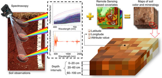
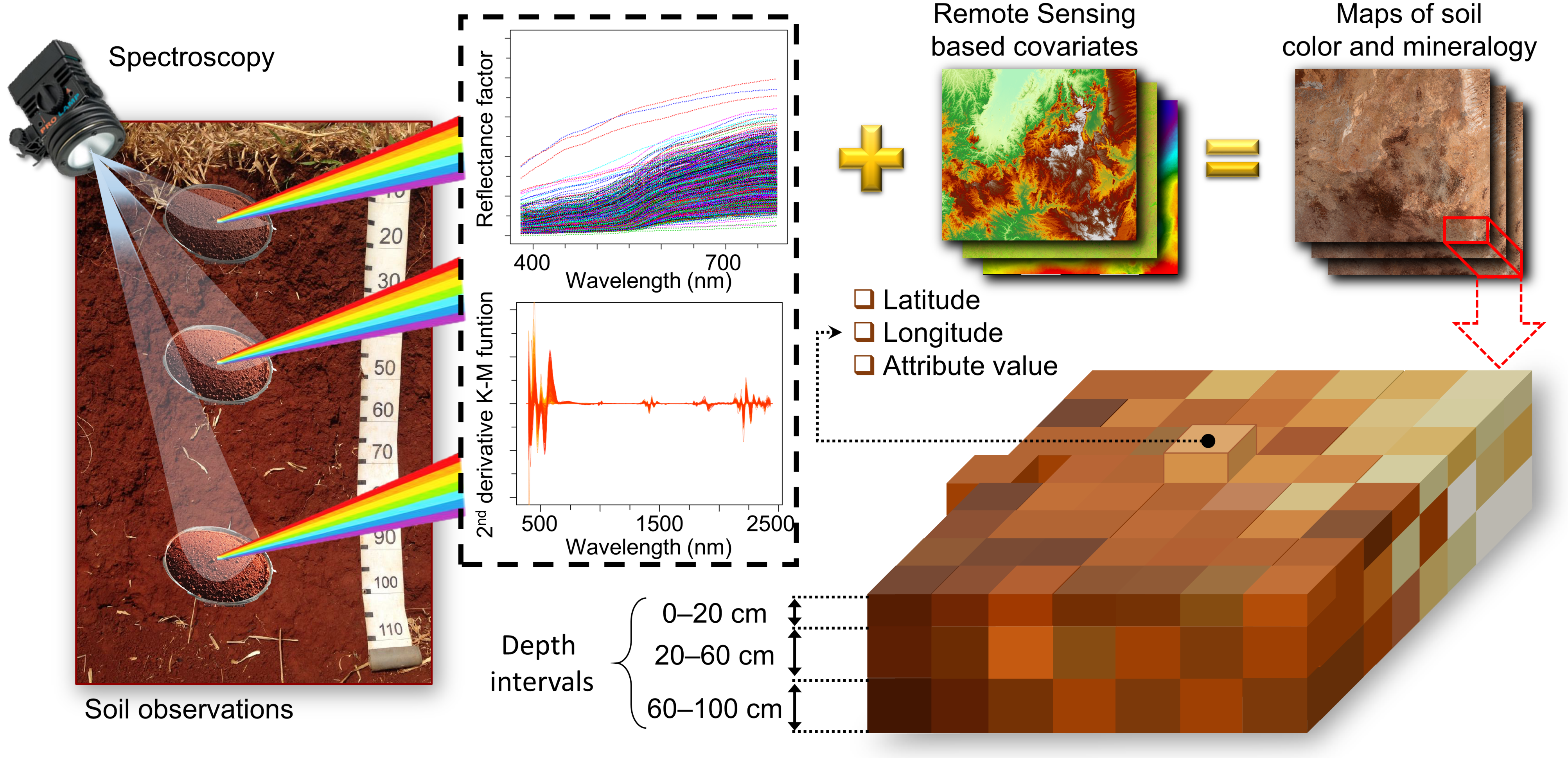
2.2. Reflectance to Soil Color

Soil scientists usually use the Munsell system to represent the soil color, resembling the natural way that humans perceive the color [8]. The Munsell notation is a cylindrical system based on three components, hue (the color, red, yellow, etc.), value (lightness), and chroma (purity, similar to saturation), which can be calculated from spectra using mathematical formulas. We used spectral reflectance data to calculate the Munsell soil color at three depth intervals (0–20 cm, 20–60, and 60–100 cm), according to Marques et al. [19] and Rizzo et al. [20]. The method used as input only the reflectance values between 380 and 780 nm (visible spectral range), and followed the steps: (1) Spectra were integrated using color-matching functions (x, y, z) to the XYZ color system for illuminant D₆₅ (daylight) and 2nd standard observer [50], (2) XYZ tristimulus values were converted to the CIELAB color system (L*a*b*), (3) coordinates a* and b* were used to calculate hue angles and chroma, while value was estimated by L*, and (4) hue angle was converted to Munsell notation using a color conversion table [51]. All steps were implemented within the R software [49], using the pracma [52] and CircStats [53] packages.

For mapping purposes, Munsell hue was converted into a numerical scale of continuous values following the arrangement of the Munsell Soil Color Book, as suggested by Hurst [15]. In this system the hue charts of interest for our soil dataset were numbered as follow: 7.5 R was 7.5, 10 R was 10, 2.5 YR was 12.5, 5 YR was 15, 7.5 YR was 17.5, 10 YR was 20, and 2.5 Y was 22.5, at 0.1 increments. The Munsell notation for selected hues (letter-number combination) used R (red), YR (yellow-red), and Y (yellow) preceded by a number from 1 to 10 to indicate position around the hue circle.

2.3. Reflectance to Soil Mineralogy

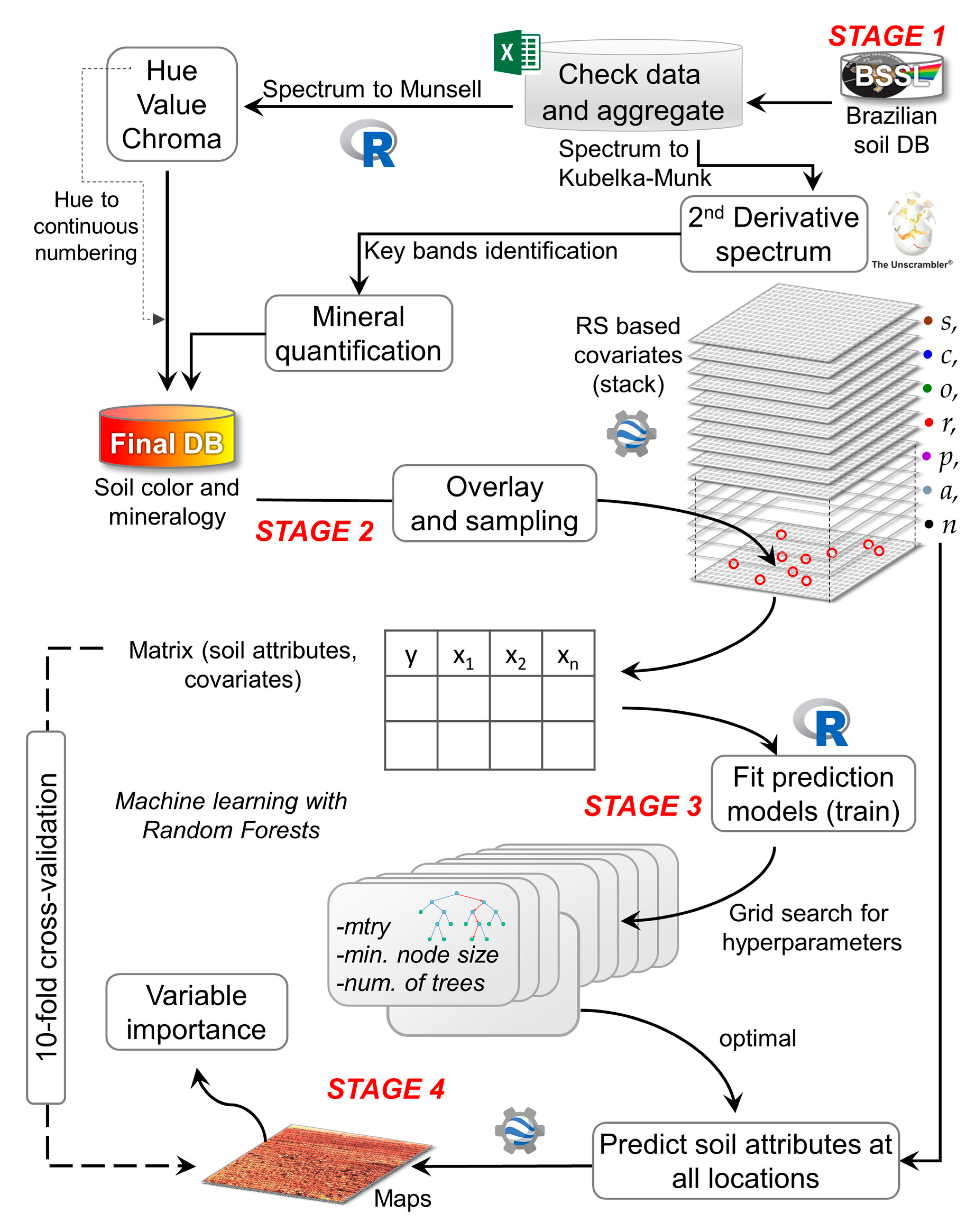
2.3.1. Spectral Processing

Soils are mixtures of mineral and organic particles which partly absorb and partly scatter the incident light. When the dimensions of the mixed particles are comparable with the wavelength of the incident light, the absorption and scattering processes can be described by the Kubelka–Munk function [$KM={\left(1-R\right)}^2/2R$, where R is reflectance] [9]. KM curves (likewise, original spectra) show broad, strongly overlapping bands at different wavelengths. Therefore, to determine the positions of these bands, the resolution may be mathematically enhanced by calculating the derivatives of the spectra. The second derivative (SD) of the KM function is a promising method for spectral quantitative analysis [54], with sensibility for soil minerals’ detection slightly smaller than X-ray diffraction [10,24]. Thus, we transformed the reflectance data of soils into the KM and then calculated the SD using Savitzky–Golay method (fitting 2nd polynomial order to 40-smoothing points), within The Unscrambler software [55]. This combination provided well-resolved spectral features and low background noise with little loss of spectral information for data collected at 1-nm intervals.

2.3.2. Key Spectral Bands for Mineral Quantification

The SD of the KM curve has spectral features originating from electronic transitions and nonfundamental vibrations of minerals [24], where minimum and maximum values match with the positions of the absorption bands in the original spectrum. The difference between derivative values at maxima and minima determines the intensity of the “band amplitude” that is equivalent to the amount of mineral in the soil sample [56]. Therefore, to assess the soil mineralogy we: (1) Selected the main minerals by checking their occurrence with previous works on soil mineralogy in the study area [57,58,59,60]; (2) defined the position of key spectral bands, at specific wavelengths ($\lambda$), for the main soil minerals, summarized in

Table 1. Position of the spectral bands in the Second Derivative (SD) of the Kubelka-Munk (KM) curve, used to calculate the amplitude for the main minerals of soils.

Soil Mineral	Minima Band Position (nm)	Maxima Band Position (nm)	Band Amplitude	Reference for Band Positions
Goethite	~415*	~455*	AGt	[24,56]
Hematite	535*	580*	AHt	[24]
2:1 clay minerals1	1900–1925	1870–1895	A2:1	[62]
Kaolinite	2205	2225	AKt	[62]
Gibbsite	2265	2295	AGb	[62]

¹ Illite, chlorite, vermiculite, montmorillonite. * Band positions relatively stable (lowest shift to neighboring wavelengths) for Al-substitution in both goethite and hematite.

, and; (3) calculated the band amplitudes for mineralogical quantification [$A=Ma{x}_{\lambda }-Mi{n}_{\lambda }$]. The intensity values of these band amplitudes were used as proxies of the soil minerals in the study area. Ternary diagrams were obtained by calculating the proportion of band amplitude between minerals for each plot using ggtern package in R [61].

2.4. Environmental Covariates

We used environmental predictors as proxies of the soil formation factors described by the scorpan model [63] for the purpose of digital soil mapping (DSM). The DSM approach assumes that a soil attribute is a function of a spatial representation of soil forming factors: Soil (s), climate (c), vegetation (o), relief (r), parent material (p), age of surface (a), and spatial position (n). Thus, we acquired a set of covariates (33 layers) from Poppiel et al. [40] to act as proxies of each factor of soil formation (

Table 2. Soil forming factor proxies from [40] used for mapping the soil color and main minerals.

Factor	Covariate	Description
Soil, Parent Material and Age	SySI	Synthetic Soil Image based Landsat 4, 5, 7 and 8 (7 bands), representing bare soil reflectance at 30 m resolution.
	Geological Lineaments	Meters of structural features per km2 from CPRM data at 1:1,000,000 scale [65].
Organisms	SyVIw and SyVId	Synthetic Vegetation Image of wet (Nov-Mar) and dry (May-Sep) seasons based Landsat 4 and 5 (7 bands), representing potential natural vegetation reflectance at 30 m resolution.
Climate	Annual Precipitation (mm)	Bioclimatic variables obtained from the WorldClim dataset at 1 km resolution [66].
	Precipitation Seasonality (CV)
	Annual Mean Temperature (°C)
	Temperature Annual Range (°C)
	Temperature Seasonality (°C)
Relief	Elevation (m)	Terrain attributes obtained from the 30 m ALOS digital elevation model [67]
	Slope (degree)
	Aspect (degree)
	Topographic Position Index (m)
	Horizontal Curvature (m)
	Vertical Curvature (m)

CV: coefficient of variation.

). These covariates were prepared using big databases of remote sensing at multiple spatial resolution within Google Earth Engine (GEE) [64]. Then, coarser-resolution predictors were downscaled into a target grid resolution of 30 m. Further details on how the covariates were prepared and quality assessed were described in [40].

2.5. Soil Modelling by Random Forest (RF)

In DSM studies [68,69,70,71,72,73,74,75], random forests [42] is increasingly being used to infer relationships between diverse soil attributes (at single and multiple depths) and several covariates (from multiple sources and resolutions) across landscapes. This fact relies on that RF can handle both linear and nonlinear relationships in data. Thus, we used RF regression for DSM of the soil color (Munsell hue, value, and chroma) and the main soil minerals (Table 1) at 0–20, 20–60, and 60–100 cm depth intervals. For that, we used the full set of covariates (Table 2) on factors of soil formation–scorpan model [63], and let the decision tree algorithm reveal the patterns. Therefore, a different model was adjusted to each soil attribute, at each one of our depths, counting 24 models. RF can fit models with large numbers of predictors [76].

2.5.1. Model Tuning

We filtered possible artifacts in the covariates (Table 2) by computing the median values within a 4 × 4 moving window. These covariates were sampled at each soil observation and the values were used as input data for calibrating RF regressions [42] using the ranger package version 0.11.1 [77] in the R software [49]. According to Probst et al. [78], a proper tuning of hyperparameters ensures the RF’s consistency. For that, we performed a grid search examining a range of values, where the number of covariates randomly selected at each node (mTry) was 6, 24, 33, and the tree depth by minimal number of samples “or leaves” for the terminal nodes (minimum node size) was 5, 20, 50. We fixed 500 trees to obtain stable estimates [78].

2.5.2. Model Performance

In order to assess the prediction models, we calculated performance metrics such as the root mean squared error (RMSE), coefficient of determination (R²), and ratio of the performance to interquartile distance ($RPIQ=\left(Q3-Q1\right)/\mathrm{RMSE}$), where Q1 and Q3 are the 1st (25%) and 3rd (75%) quartiles. The RPIQ is based on prediction error and quartiles, which evaluate the spread of the dataset to the model’s accuracy, making easier the comparison among soil attribute models and other studies. We derived these metrics for each one of the 24 models to assess the goodness of fit in the calibration step, and the robustness in the validation step. Validation was performed for each one of the 24 models by 10-fold cross-validation, using the caret package version 6.0-84 [79]. The k-cross-validation maximizes the quantity of points in the training dataset, where the points are divided into k groups or folds, where k − 1 groups are used for training and 1 group for validation, repeating the training k times, each with a different validation group [80]. We selected the optimized model by the minimum RMSE of the 10-fold cross-validation [78,81]. Generally, smaller values of RMSE and larger R² and RPIQ indicate higher model performance [82].

2.5.3. Covariates’ Importance

RF models can be interpreted by providing measures for variable importance [68,69,70,71,72,73,74,75], based on the increase in mean square error when a covariate is randomly permuted. Thus, we used the folds estimates to calculate the mean frequency of use for the covariates in the models and reported as a measure of the scaled permutation importance for each soil attribute prediction [42], using the ranger package version 0.11.1 [77] in R [49]. Interpreting this output is quite straightforward: The more importance, the more relevant the variable is, according to the model.

2.5.4. Soil Mapping

The optimized models (tuned hyperparameters in R) of soil attributes were implemented into the cloud-based platform of GEE [64] to predict their spatial distribution in the study area using the RF algorithm. In this study, the uncertainty was not examined as maps because this technique was not implemented at the current development stage of GEE [64]. Therefore, to verify the correspondence of the spatial patterns of our predictions, we performed Pearson’s correlation between our maps (at the three depth intervals) with legacy soil observations acquired from a national dataset [33], and also with weathering degree and hue, both inferred according to the World Reference Base for Soil Resources – WRB [14] from a 1:1,000,000-scale legacy soil class map that covered the study area [45]. The flow diagram of the proposed method is shown in Figure 2.

3. Results

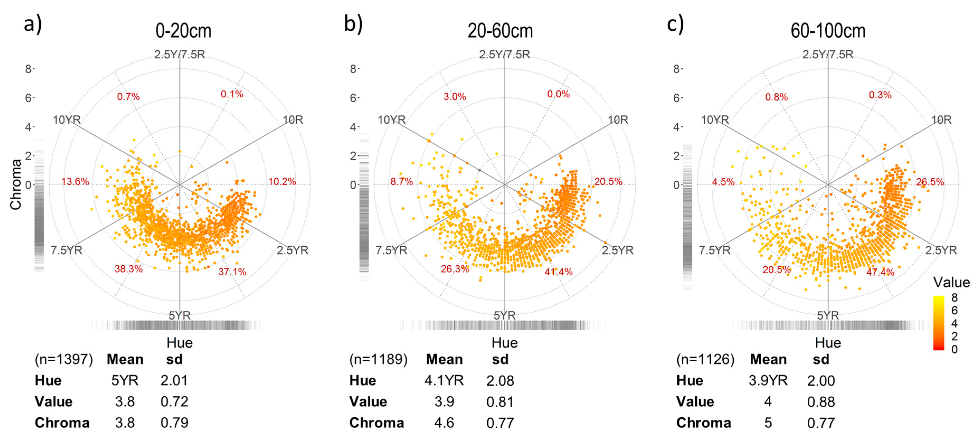
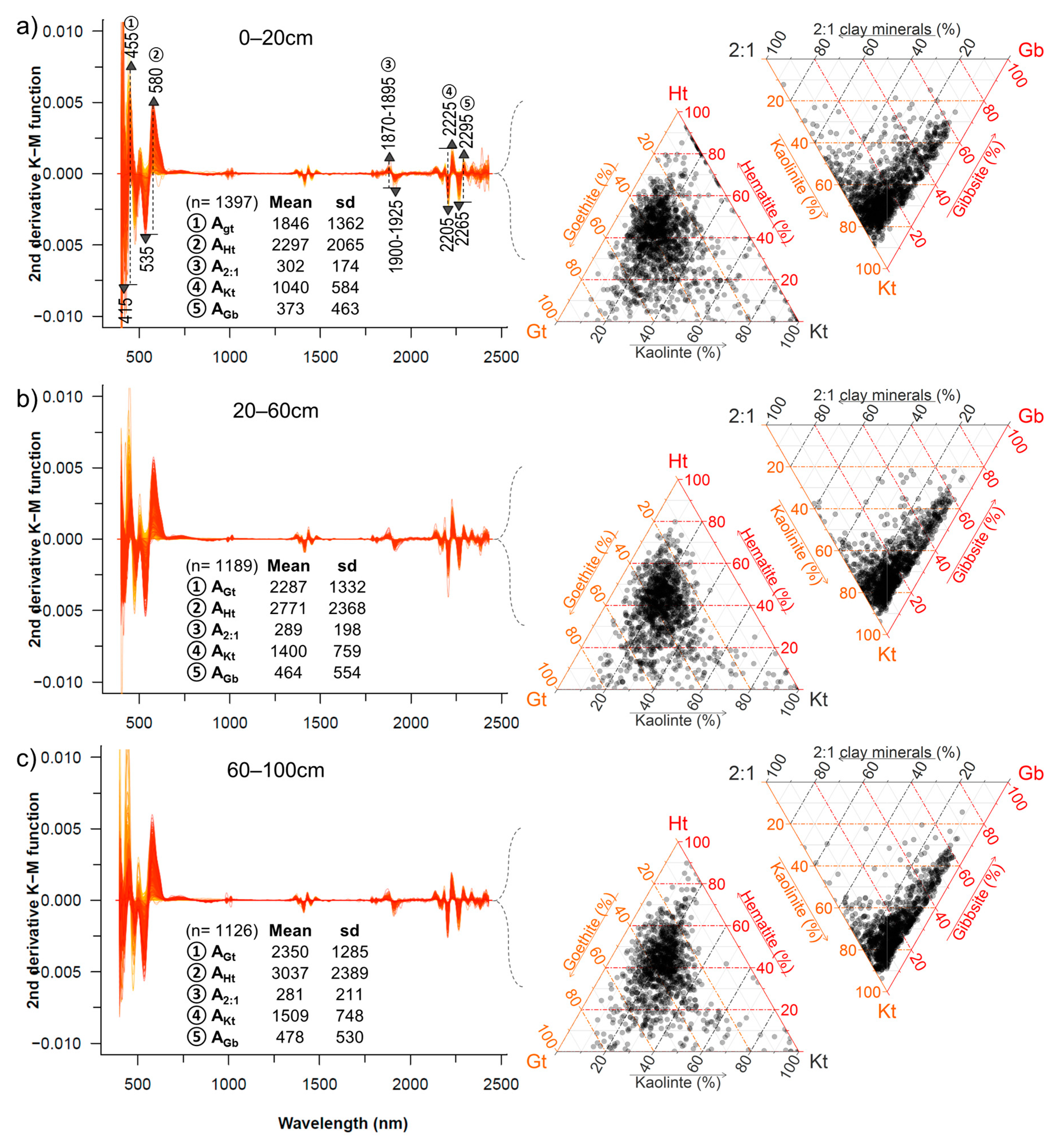
3.1. Soil Attributes Derived from Spectra

Spectra (350–2500 nm) contain information on important attributes of the soil: Minerals, color, organic material, texture, and water. The reflectance in the visible spectral interval revealed that in our dataset the soil color ranged from 8.9 R (red) to 2.5 Y (yellow), and reached more than 50% of samples up to 5 YR (yellow-red) (Figure 3). Value and chroma ranged from 1.7 to 8 and from 0.7 to 8 with mean values of 3.9 and 4.5, respectively. Overall, the hue decreased and the value and chroma increased as the soil depth interval increased. That is, the soil color was redder, lighter, and purer (or saturated) at deeper layers. The amplitude between key spectral bands in the SD KM curve (Table 1) indicated that the soils were dominated by hematite, goethite, and kaolinite, with relative amounts between them of about 38%, 36%, and 25%, respectively. These minerals were mixed in soils with smaller amounts of gibbsite and 2:1 clay minerals, where its proportions in relation to kaolinite were near 19%, 15%, and 66%, respectively (Figure 4).

The significant (p < 0.01) Pearson’s correlations for goethite (−0.3 < r < −0.66) and hematite (−0.79 < r < −0.88) with hue and value suggested that iron oxides decreased these color attributes and promoted the redness and darkness of the soils at the three depth intervals (Figure 5). Iron oxides also were correlated with chroma (average r of 0.29), which caused the saturation of soil color.

All minerals were positively correlated with each other (Figure 5a–c), where gibbsite and 2:1 clay minerals showed the smallest values between them (r < 0.21). Likewise, the proportion of minerals slightly increased with depth (Figure 5d), since they are relatively dominant at finest fractions, and there is more clay in the subsurface of the studied soils. Gibbsite was relatively constant across depth (Figure 5d), while the 2:1 clay minerals were a little more abundant in the topsoil. The hue decreased with depth while chroma increased, both due to small amounts of iron oxides, which pigmented the soil at deeper layers. Value increased with depth (Figure 5d), since it depends on reflectance, which increases with lesser amounts (masking effects) of organic matter on mineral particles.

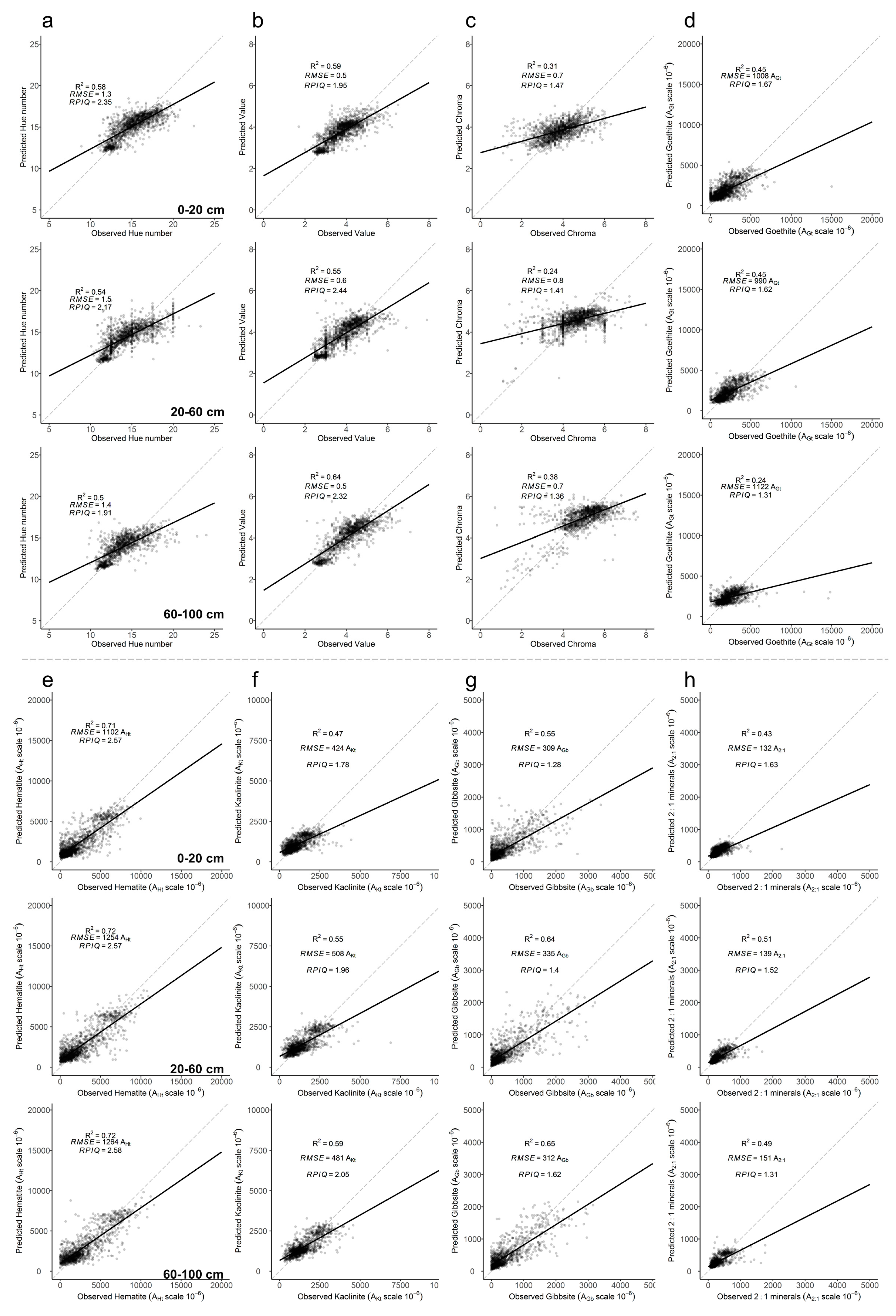
3.2. Performance of Spatial Models

The RF models proved to be robust for mapping soil color and mineralogy at three depth intervals in Midwest Brazil (

Table 3. Hyperparameters and performance metrics for calibration (goodness of fit) and validation (robustness) of the models used for mapping soil attributes at surface and subsurface.

Soil Attribute	Depth2	mTry	minNS	RMSEcal	RPIQcal	R2cal	RMSE10cv	RPIQ10cv	R210cv
Hue number1	0–20	24	5	0.53	5.89	0.93	1.30	2.35	0.58
	20–60	24	5	0.61	5.45	0.93	1.50	2.17	0.54
	60–100	33	5	0.56	4.80	0.92	1.40	1.91	0.50
Value	0–20	24	5	0.19	4.84	0.93	0.50	1.95	0.59
	20–60	24	5	0.24	5.85	0.92	0.60	2.44	0.55
	60–100	24	5	0.21	5.79	0.94	0.50	2.32	0.64
Chroma	0–20	33	5	0.27	3.67	0.89	0.70	1.45	0.31
	20–60	33	5	0.31	3.56	0.88	0.80	1.41	0.24
	60–100	33	5	0.29	3.41	0.90	0.70	1.36	0.38
Goethite	0–20	24	5	414*	4.07	0.91	1008*	1.67	0.45
	20–60	24	5	396*	4.06	0.91	990*	1.62	0.45
	60–100	6	5	494*	2.97	0.85	1122*	1.31	0.24
Hematite	0–20	24	5	436*	6.49	0.96	1102*	2.57	0.71
	20–60	24	5	496*	6.49	0.96	1254*	2.57	0.72
	60–100	24	5	504*	6.46	0.96	1264*	2.58	0.72
Kaolinite	0–20	33	5	171*	4.41	0.91	424*	1.78	0.47
	20–60	33	5	205*	4.86	0.93	508*	1.96	0.55
	60–100	33	5	190*	5.20	0.94	481*	2.05	0.59
Gibbsite	0–20	24	5	123*	3.23	0.93	309*	1.28	0.55
	20–60	33	5	132*	3.55	0.94	335*	1.40	0.64
	60–100	24	5	124*	4.09	0.95	312*	1.62	0.65
2:1 minerals	0–20	33	5	54*	3.99	0.90	132*	1.63	0.43
	20–60	24	5	56*	3.75	0.92	139*	1.52	0.51
	60–100	24	5	63*	3.13	0.91	151*	1.31	0.49

¹ See Munsell hue in Section 2.2. ² Depth in cm. * Scale factor 1 × 10⁻⁶. The mTry: Hyperparameter of random forest regression that controls the number of variables that can be randomly sampled in each split of the trees. The minNS: Minimum node size, a hyperparameter of random forest that controls the tree depth by setting the minimal number of samples for the terminal nodes. RMSE_cal: Root mean square error of calibration. RMSE_10cv: Root mean square error of 10-fold cross-validation. R²_cal: Coefficient of determination of calibration. R²_10cv: Coefficient of determination of 10-fold cross-validation.

), with high prediction accuracy for hematite (R²_10cv > 0.71). The prediction of Munsell value and hue, gibbsite, kaolinite, 2:1 minerals, and goethite was accurate (0.43 < R²_10cv < 0.65). The models for goethite produced lower validation metrics than for hematite (Table 3), especially at 60–100 cm depth (R²_10cv = 0.24), probably because the first had higher Al-substitution that affected the spectral bands used for their relative quantification (Table 1). Munsell chroma at all depths had worse prediction accuracy (0.24 < R²_10cv < 0.38). Although some models had low R² for validation, they all showed a good performance (RPIQ_10cv > 1.3) and scatterplots with values following linear trends (Figure A1).

3.3. Relevance of Covariates

The importance of each covariate on predicting Munsell color and mineralogy of soil is shown in Figure 6. The main predictors (global importance > 10%) for most of the attributes and depths of soil in the study area were (decreasing sequence) SySI_Blue, elevation, annual precipitation, temperature annual range, temperature seasonality, SySI_Green, SYSI_Swir2, annual mean temperature, SYSI_NIR, precipitation seasonality, SySI_Red, topographic position index and SySI_Swir1. These covariates remained unchanged and usually in the same sequence at each depth, with bare topsoil reflectance at the blue spectral region (SySI_Blue) as the most relevant predictor for our conditions. They are proxies of the soil forming factors s, c, r, p, and a (Table 2), which all interact to influence spatial distribution of color and minerals of soil in Midwest Brazil.

The forming factor o, represented by the potential natural vegetation reflectance of dry and wet seasons, especially at blue, green, red, and near-infrared spectral ranges, had medium to low importance (global < 10%) to predict soil color and mineralogy at all depths (Figure 6). The reason is that vegetation had a more local effect on the spatial distribution of soil attributes, followed by slope and density of geological lineaments. Horizontal and vertical curvatures had low importance, while aspect was frequently not important as predictor for our conditions (Figure 6), possibly because the sparse and uneven distribution of our soil dataset failed to describe important short-range patterns of soil variations contained in these covariates.

3.4. Digital Maps of the Soil Surface and Subsurface

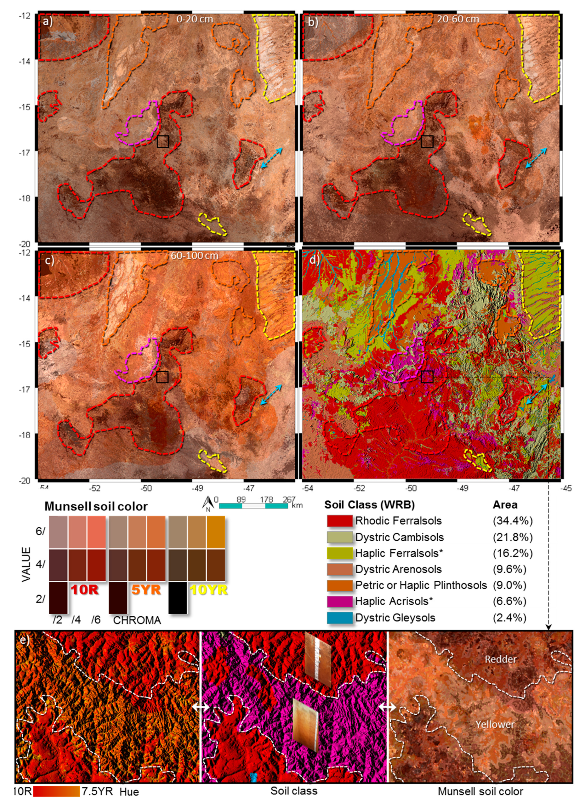
3.4.1. Gridded Munsell Soil Color

We used the maps of Munsell hue, value, and chroma to obtain RGB (Red, Green, Blue) composites of the true Munsell color of soil for the three depth intervals (Figure 7). It allowed us to simultaneously assess and compare the spatial patterns of the three components.

On average, the study area had 49% of soils with hues redder (lower) than 5 YR across the three depths (Table 3), which were mainly represented by Rhodic Ferralsols (and some Rhodic Nitisols and Acrisols of lower occurrence), followed by some Dystric Cambisols and Petric Plinthosols with redder hues in the soil matrix (see areas highlighted with red dashed lines in Figure 7). Within this set of soils, 7% were redder than 2 YR, due to the presence of ferralic (also ferritic) horizon of some Ferralsols (and Nitisols or Acrisols) developed from basalt in the study area.

About 51% of soils of the study area had Munsell hues yellower (higher) than 5 YR up to 100 cm depth, which were represented by Haplic Ferralsols, Haplic Acrisol, Arenosols, Haplic Plinthosols, and Petric Plinthosols with yellower matrix (see areas highlighted with yellow dashed lines in Figure 7). Among these soils, 7% exhibited hues yellower than 7.5 YR due to: (1) Lower ratio of hematite/(hematite+goethite), where higher contents of goethite pigmented the soil, such as in Xanthic Ferralsols, or (2) reduction and removal (or partial removal) of iron oxides from Gleysols.

The orange dashed lines in Figure 7 highlight areas with Plinthosols (mainly Petric) in the study area. These soils contain petroplinthite (rich in Fe and Al) within a latosolic matrix, which can range from yellowish (10 YR) to reddish (10 R), according to the parent material. Their hue also can vary across the same soil profile. This features are important to understand the maps, because in such areas the Munsell color was more changing between depths.

The maps (Figure 7) showed that most of the soils in the study area with hues between 2.5 YR and 7.5 YR became redder with depth (

Table 4. Area quantification of the Munsell soil hue maps at three depth intervals.

Depth	Hue < 2.5YR	2.5YR ≤ Hue < 5YR	5YR ≤ Hue ≤ 7.5YR	7.5YR < Hue
(cm)		Area (%)
0–20	1	27	66	6
20–60	4	49	46	1
60–100	16	49	23	13
Average	7	42	45	7

). In addition, soils with Munsell hues <5 YR usually presented lower values and higher chromas than yellower soils with hues ≥5 YR. The predicted true color of soils showed a comprehensible spatial correspondence with taxonomic classes of the legacy soil map. It can be observed in detail in Figure 7e, where the distinction of the spatial pattern of hue and true soil color is clearly evident between a Rhodic Ferralsol (redder and darker) and a Haplic Acrisol (yellower, lighter, and brighter).

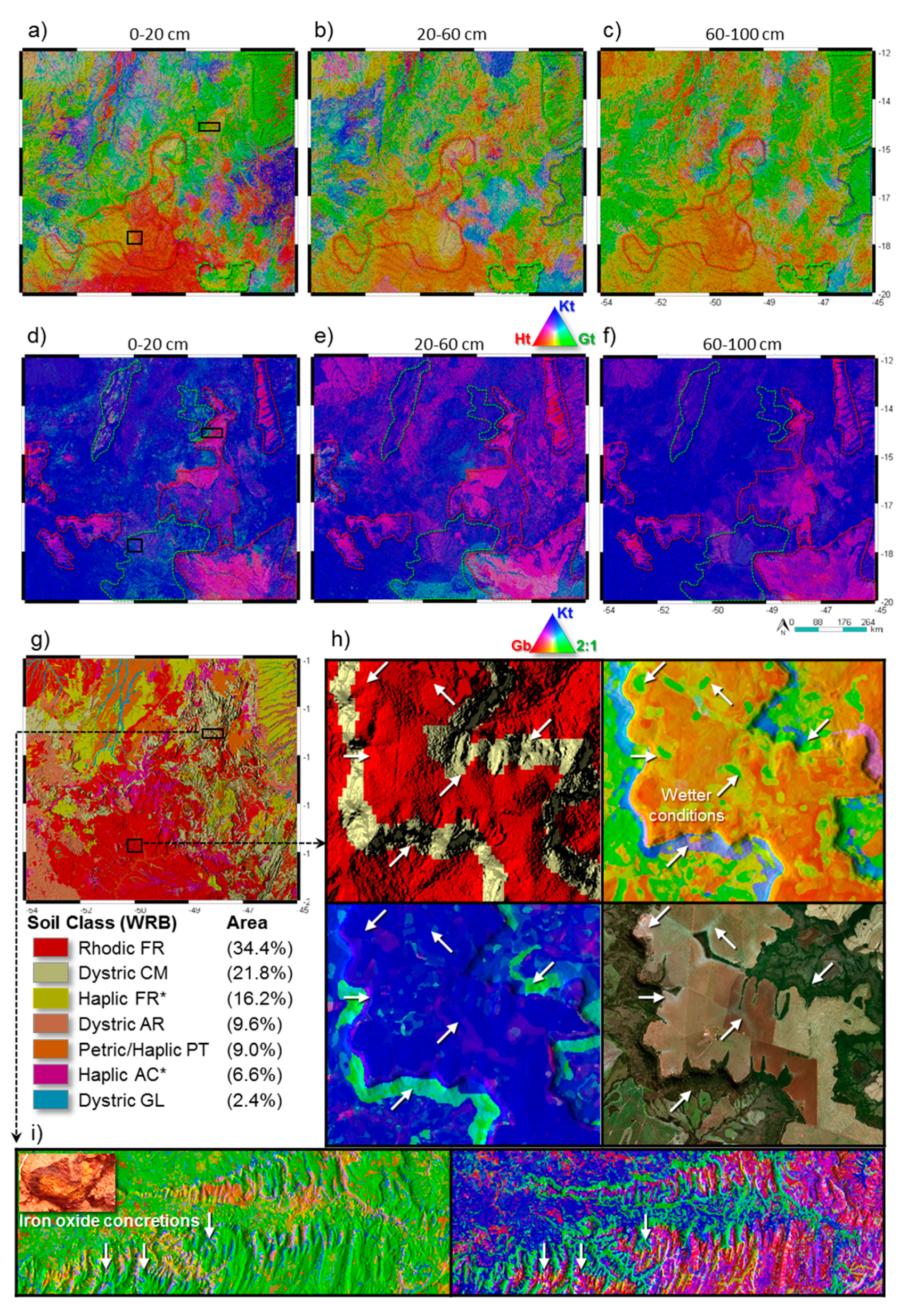
3.4.2. Spatial Patterns of the Main Minerals in Studied Soils

For simultaneous assessment of the spatial patterns of soil mineralogy at each depth, we separately obtained RGB compositions for hematite, goethite, and kaolinite (Figure 8a–c), and for gibbsite, 2:1 clay minerals, and kaolinite (Figure 8d–f).

More than 50% of the study area was covered by highly weathered soils with high relative proportions of hematite, goethite, and kaolinite, followed by gibbsite and 2:1 clay minerals (

Table 5. Area quantification of the soil mineral maps at 0−20, 20−60, and 60−100 cm depth intervals.

Relative Amount1	0−20 cm	20−60 cm	60−100 cm	Average
(%)		Area (%)
9 < Ht ≤ 31	51	48	42	47
31 < Ht ≤ 49	36	46	52	45
49 < Ht ≤ 66	13	5	6	8
6 < Gt ≤ 24	23	12	6	14
24 < Gt ≤ 37	55	69	72	65
37 < Gt ≤ 50	22	19	23	21
4 < Kt ≤ 19	46	44	43	44
19 < Kt ≤ 31	34	38	50	41
31 < Kt ≤ 50	21	17	7	15
1 < Gb ≤ 9	69	63	60	64
9 < Gb ≤ 17	26	20	38	28
17 < Gb ≤ 29	5	17	2	8
2 < 2:1 ≤ 7	58	79	91	76
7 < 2:1 ≤ 13	34	20	9	21
13 < 2:1 ≤ 18	8	0.4	0	3

¹Amount of given mineral in the < 2 mm fraction of soils. Gt: goethite; Ht: hematite; Kt: kaolinite; Gb: gibbsite; 2:1: 2:1 clay minerals.

). The relative proportions of iron oxides in the soil ranged from 6% to 66%, as the surface materials were Fe rich. The highest proportions of hematite (49% < Ht ≤ 66%) were found in 8% of soils, that accounted for nearly 7% of soils with hues redder than 2.5 YR (Table 3). About 45% of soils had hematite contents ranging from 31 to 49% (see areas with red dashed lines in Figure 8a–c, and Table 5), that agreed with ~42% of soils with reddish hues between 2.5 YR and 5 YR (Table 4). This iron oxide also occurred in 47% of soils at lower contents (9% < Ht ≤ 31%), possibly coexisting with most of the 65% of soils with goethite amounts ranging between 24% and 37%, that may account for ~45% of soils with yellowish hues ranging from 5 YR to 7.5 YR. The lowest amounts of goethite, ranging from 6% to 24%, might be distributed in the redder soil masked by pigmenting effects of hematite. Conversely, 21% of soils presented high amounts of goethite ranging between 37% and 50% (see areas with green dashed lines in Figure 8a–c, and Table 5), which may account for the color of soils with hues yellower than 7.5 YR.

The study area had about 56% of soils with high kaolinite contents ranging from 19% to 50% (blue shades in Figure 8d–f), which seemed to coexist in equilibrium with most of the 64% of soils with low amounts of gibbsite (1% < Gb ≤ 9%). On the other hand, a large proportion of weathered soils (44%) with low kaolinite contents (4% < Kt ≤ 19%) might coexist with the 36% of soils with the highest gibbsite contents, ranging from 9% to 29% (see areas in shades of magenta with red dashed lines in Figure 8d–f, and Table 5). These highly weathered soils were typical on highland surfaces, where long-term weathering resulted in intensive leaching of silica from soil particles.

Traces of 2:1 clay minerals (<7%) were found in most of soils in the study area (76%), while the remaining 24% of soils showed higher contents (7% < 2:1 ≤ 18%), displayed with shades of cyan in Figure 8d–f (especially in areas highlighted with cyan dashed lines). Table 5 shows that iron oxides and kaolinite contents increased with depth, while gibbsite increased with less intensity. Higher proportions of 2:1 clay minerals seemed to be more abundant at topsoil.

We show in detail the spatial patterns of soil mineralogy in two expanded areas linked to the legacy soil map (Figure 8g). The first area (Figure 8h) was on a highland plateau developed upon arenite and covered by Ferralsols, where flat areas in red shades were predicted with redder color (3 YR 3/5) and proportions of Ht = 46%, Gt = 36%, Kt = 10%, Gb = 5%, and 2:1 = 3%, indicating that hematite was dominant in well-drained conditions. Concave areas or lower slopes surrounding drainages with green shades in the map (marked by black arrows) showed yellower color (6 YR 4/4) and proportions of Ht = 27%, Gt = 47%, Kt = 18%, Gb = 3%, and 2:1 = 6%, suggesting that goethite was dominant in wetter drainage conditions. Conversely, plateau edges covered by Cambisols with cyan shades in the map, presented color 3 YR 4/3 and amounts of Ht = 38%, Gt = 36%, Kt = 8%, Gb = 2%, and 2:1 = 16%, suggesting less weathered conditions and younger soils.

The second area (Figure 8i) presented two scenarios. One was developed upon siltite, where smoother relief (shades of blue) showed color 5.5 YR 4/5 and proportions of Ht = 30%, Gt = 40%, Kt = 15%, Gb = 5%, and 2:1 = 10%, suggesting less weathered conditions. Areas over ferruginous laterite crusts with hilly relief (shades of magenta), and occurrence of iron oxide concretions, presented color 7 YR 4/4 and amounts of Ht = 16%, Gt = 43%, Kt = 8%, Gb = 29%, and 2:1 = 4%, indicating highly weathered conditions on an ancient surface. Thus, the first scenario accounted for younger soils (e.g., Cambisols), while the second corresponded to older soils, such as Petric Plinthosols.

4. Discussion

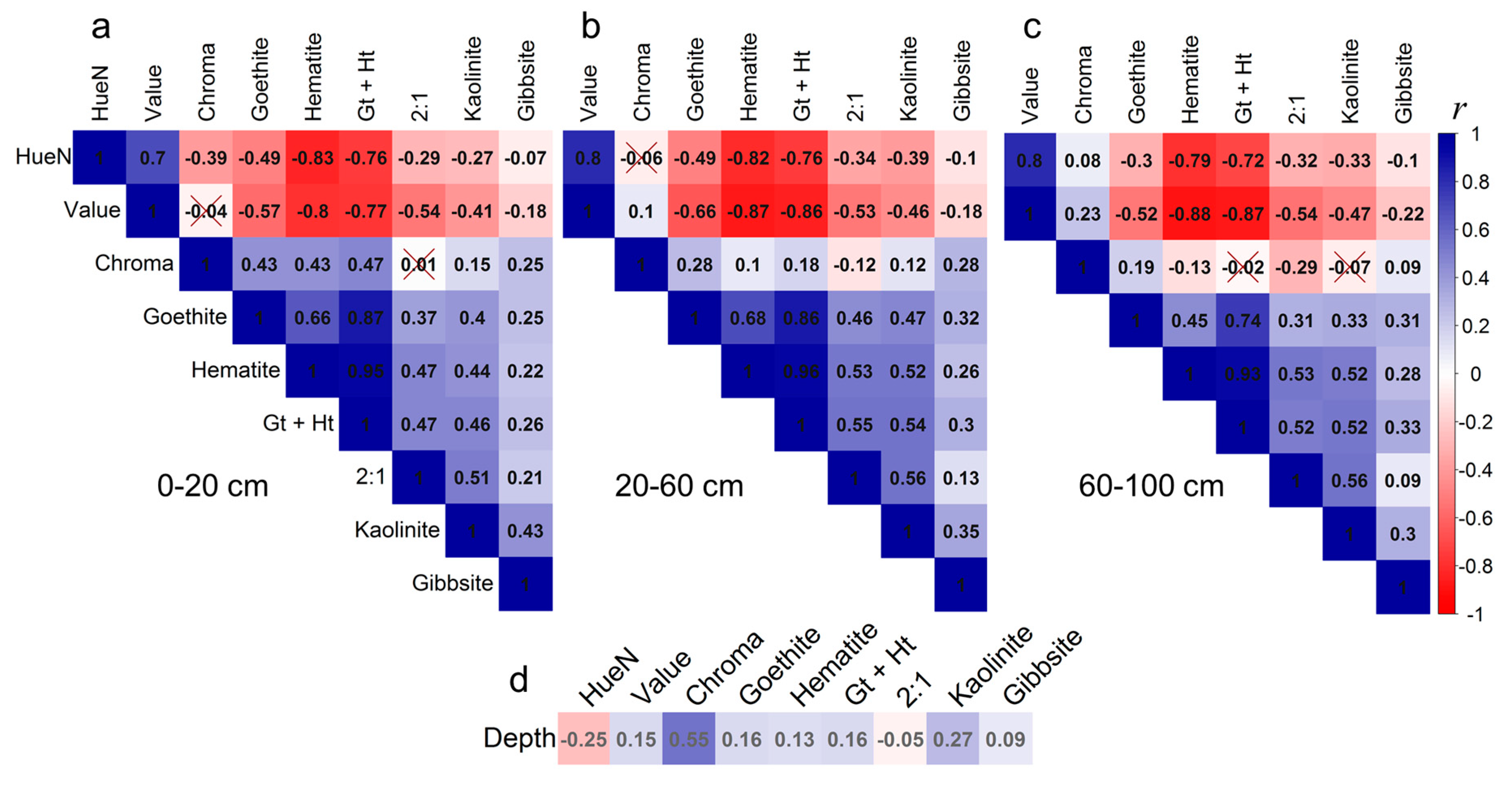
4.1. Relationships Between Soil Color and Mineralogy

We did not verify the accuracy of the color estimations at each site because: (1) We lacked colorimeter records in our dataset; (2) spectral data were acquired under the same conditions as in reference works [19,20]; and (3) the mathematical procedures of reference, implemented in this section, provided similar color estimations to the colorimeter measurements, with R² ranging from 0.68 to 0.96 and RMSE between 0.19 and 0.57 [19,20].

Aitkenhead et al. [2] demonstrated that inherent color of soil is mainly controlled by organic compounds and iron oxides. Soil organic matter causes the darkness of soil by decreasing the Munsell value and chroma [4]. Poppiel et al. [40] found organic matter inversely correlated (r = -0.4) with soil depth for the same area of Brazil, where average content ranged from 21 g kg⁻¹ at the surface to 9 g kg⁻¹ in the 60–100 cm depth. These findings agreed with our results, where value and chroma increased with depth, while organic matter decreased, suggesting a negative correlation between them, as reported by [18].

The most frequent pedogenic oxides in tropical soils are hematite (usually associated to goethite) with hues between 10 R and 5 YR, and goethite that has hues between 7.5 YR and 2.5 Y [3]. Munsell color varies with mineral concentration, where higher contents reduce the value and increase the chroma of soil [83]. According to the geodiversity of the region [6], the most surface materials (Figure 1) contain Al, Si, and Fe-bearing minerals that released these elements during their weathering (hydrolysis) and it favored the formations of oxide pigments (e.g., hematite and goethite) [1], common to the majority of the studied soils (Figure 3) [59,84,85,86]. Goethite (FeOOH) usually occurs in wetter, colder, and more acidic (pH 4) pedoenvironments, with seasonal anaerobic conditions and slow Fe release [1]. When the pedoclimate becomes drier, warmer, and less acidic (pH higher than 4) under higher Fe release, the ferrihydrite (precursor) is formed and then dehydrated to hematite (Fe₂O₃), or, also, goethite can dehydrate to hematite [3]. Usually, in red soils widely distributed in our study area (e.g., Rhodic Ferralsols), the yellowish hues (10 YR) of coexisting goethite are masked by the higher pigmenting effects of hematite with reddish hues (10 R) [9]. Hematite, a less stable mineral, is generally negligible or absent in yellow soils (e.g., Xanthic Ferralsols) from the Central Plateau of Brazil [5].

When iron oxides are completely removed (after mobilization by microbial reduction) under anaerobic conditions from soil particles, and if organic matter is negligible, the soil achieves the base color of the matrix minerals resulting in shades of gray (gleyic) [3]. Reducing conditions can dramatically reduce the chroma and increase the value of gleyed horizons, suggesting saturation by water in concave areas of the landscape, characteristic of Gleysols [14].

The highest kaolinite content in the <2 mm fraction of soils (see ternary graphs in Figure 4) might result from primary minerals, which weathered directly into kaolinite under intense warm and wet leaching in tropical conditions [87]. Gibbsite, a pedogenic Al(OH)₃, is formed by desilication of kaolinite or primary minerals, at low silica concentration and low pH (5-6), when leaching rates are rather high in well-drained tropical soils [7]. Relatively large amounts of this mineral were found in the clay fraction of deeply weathered soils in central Brazil [86].

The 2:1 minerals are derived from their parent materials and can be present: (1) In the clay fraction along the profile of younger (less weathered) soils, or (2) strongly interlayered with Al in older soils, which decrease the cation exchange capacity by blocking exchange sites and provide greater stability, as reported by some works for the same region [59,84,85]. In addition, weathered soils (e.g., Ferralsols) can contain up to 5, 17, and 5% of 2:1 minerals in the sand, silt, and clay fractions, respectively [86]. The first two fractions slightly decreased their concentration with depth in the region [40], and, therefore, the 2:1 minerals were reduced as well (Figure 4 right panels and Figure 5d).

Soil color allows us to infer about the conditions of aeration and drainage of the soil and, consequently, of pedogenetic processes. Thus, red soils (hematite and goethite) are in well-drained interflows, yellow soils (goethite), on moderately drained slopes, and grey soils develop in poorly drained foothills. Mineralogical composition can be used to estimate the degree of weathering of soils, where the next sequence indicates an increasing degree of evolution (from younger to older): 2:1 < kaolinite < hematite < goethite < gibbsite. Thus, the majority of soil presented an advanced weathering degree with good drainage condition, developed in flattened or smoothed reliefs.

4.2. Use of Regression Models for Mapping Soil Properties

As soil color and mineralogy are important proxies used to distinguish different soil types or to infer related soil attributes [17], they play an important role in soil cartography. Some studies have used reflectance spectroscopy (350–2500 nm) as input data to estimate the color and/or its mineralogy [18,19,20,21,22,23,24], but only a small number of works mapped their spatial distribution. At the moment, Viscarra Rossel et al. [25] performed one of the few studies on soil color mapping, where they accurately mapped (R² ≅ 0.67) iron oxides and the color of Australian soil using reflectance spectra (350–2500 nm) and geostatistics.

Studies on mapping the soil mineralogy, such as Viscarra Rossel and Chen [26], summarized the information content of spectra (350–2500 nm) by principal components to construct linear models, and map the mineral (the first three principal component scores) of Australian topsoils robustly (0.69 < R²_10cv < 0.85). Likewise, Viscarra Rossel [27] measured the relative abundances of kaolinite, illite, and smectite at 0–20 and 60–80 cm soil depths, using continuum-removed reflectance (350–2500 nm) to derive statistical models and map the minerals with good cross-validation results (0.40 < R²_10cv < 0.61). Malone et al. [28] also used continuum-removed spectra (350–2500 nm) for the detection of iron oxides, kaolinite, and smectite prior to mapping their spatial distribution in Australia, such as ordinal classes at fixed mineral abundance intervals, with overall accuracy ranging from 44% to 80%. Mulder et al. [29] used reflectance spectroscopy (350–2500 nm) to derive soil minerals, and multinomial logistic regression, for mapping the likelihood of “absence” or “presence” of kaolinite, mica, and smectite with high overall accuracy (>0.74). Other studies [30,31,32] used enhanced mineral mapping techniques to produce a thematic mineral map of soil using the spectral response of Landsat imagery.

Our performance metrics were consistent with studies mentioned above, where most of them used scorpan model [63] for DSM and reported a decline of prediction accuracy from calibration to validation, as summarized in Table 3. The unexplained part of soil variation in our study area can be due to two aspects. The first might be a limited number of sparse soil observations, with one site per ~2 km² (denser) to ~800 km² (less dense) and ~600 km² on average in the study area, as also reported by Liu et al. [88] when they mapped the texture of Chinese soils using RF algorithm. This may be not sufficient to capture and describe short-range patterns of soil variation [89]. The second, and the most relevant for soil mapping and its cross-validation, can be an uneven spatial distribution of observations [73]. In large-extent mapping, more landscapes are usually included with sampling sites not uniformly distributed over space. Figure 1 shows that the northwestern and northeastern portions of the study area had less soil observations than other parts. That is because: (1) the soil data used in this study were acquired by survey activities with limited funding, along different periods of time, and without a statistical design, but purposive; and (2) a relatively smaller soil spatial variation in the northwestern and northeastern, developed over more uniform conditions of geology and relief, were considered by our observations.

Despite our dataset covering the main soil-landscape conditions across the study area, 10-fold cross-validation was performed on uneven distribution of observations. This method selects 10% of total sites for validation, leading to a relatively smaller amount of data for modelling in the areas with sparse observations [88]. In addition, although the model performances were robust for the whole extent, its prediction may have been biased in local areas.

The worse spatial prediction accuracy for chroma can be a consequence of a possible lower performance in their determination from spectra, since this Munsell component is influenced by the organic matter, which decreases in depth, where chroma model had a slightly better performance (R²_10cv = 0.38). In addition, Liles et al. [90] reported that soils developed over sedimentary rocks, as was most of our study area, showed an increasing in the coefficient of variation for Munsell chroma. Silva et al. [10] found that the spatial variability of goethite was about twice higher than hematite in soils from the Western Paulista Plateau of Brazil, strongly influenced by the parent material. Thus, the lowest model performance for chroma may be related to effects of the density and locations of soil observations used for color predictions, combined with the high occurrence of sedimentary parent materials in the study area.

The substitution of Fe by Al in goethite, that is greater than in hematite, ranging from 7% to 40% for Brazilian soils [7], may produce their lower performance. This process causes less stability in the absorption feature of goethite [24,56] and, consequently, lower prediction performances, especially at subsoil layers (R²_10cv = 0.24), where we had a relatively smaller number of soil samples.

4.3. Influence of Environmental Predictors in Soil Color and Mineralogy Patterns

Most influential covariates were important predictors of the soil color and mineralogy because they captured the soil spatial patterns at shorter distances or local variations (detail), and also at longer distances or regional variations (generalization) across different landscapes [89]. Therefore, SySI (soil), SyVI (vegetation), elevation, and derived relief attributes describe at detail the factors of soil formation, while temperature, precipitation, and geological lineaments generalized their patterns [27]. Then we were able to spatialize our soil predictions from detailed to successively coarser levels of generalization in our study area. The impact of using multi-scale and multi-source predictors for modelling soil attributes was demonstrated by [91]. They reported that the parallel use of covariates at multiple levels of spatial representation for DSM improved the model performance, promoting R² increases of up to 70%.

Studies can take advantages from the petabyte-scale Landsat datasets widely available within GEE [64]. The covariates SySI and SyVI (Table 1) are examples of that [40], which provide improved proxies for describing several soil forming factors, e.g., s, o, p, and a [63]. SySI can provide direct and interpretable information from Earth bare surfaces, from which inferences can be made about the main soil attributes, e.g., the soil color, mineralogy, and texture, among others [39,40]. In a recent study, Roberts et al. [30] robustly estimated the spectral response of the bare surfaces using the full temporal archive of Landsat images across Australia. The authors highlighted the broad application of the topsoil reflectance mosaic, which can be combined with machine learning for enhanced geological mapping, mineral exploration, and digital soil mapping. Likewise, Post et al. [92] reported a very strong correlation (0.68 < r < 0.85) between Munsell soil color measured with a colorimeter and Landsat reflectance on semiarid rangelands, where they precisely and accurately determined the color of bare topsoil using remotely sensed spectral data.

When we examined individually the relevance of predictors for each soil attribute, we found that SySI_Blue, SySI_Green, and SySI_Red, were the most important spectral bands to predict Munsell hue (from 12 to 47%), value (from 14 to 34%), and chroma (from 11 to 26%), see Figure 6. This is because the Munsell color system described different soil components with absorption features (due to electronic transitions) in the visible range between 380 and 780 nm [8], where the blue, green, and red Landsat spectral bands are situated. The SySI_Blue was by far the most important predictor for geothite (from 7 to 34%) and hematite (from 47 to 60%), followed by SySI_Green and SySI_Red (between 8 and 22%). Goethite and hematite had stronger absorption features situated between the blue and red spectral ranges (Figure 4), with a weaker effect in the near-infrared interval [24,56]. The SySI_Swir1 and SySI_Swir2 were important (from 9 to 37%) for gibbsite and kaolinite because they both exhibit molecular vibrations (involving stretching and bending) between ~1400 and ~2300 nm [62]. Also, SySI_Blue and SySI_NIR were important (from 11 to 21%) for gibbsite and kaolinite, because these minerals are usually associated with iron oxides in tropical soils [1,7], which had spectral response between 380 and 1000 nm [24,56]. SySI_Swir2 was important (from 8 to 12%) for predicting 2:1 clay minerals, due to their typical absorption features (by molecular vibrations) near 1900 nm [62]. SySI_Blue, SySI_Green, and SySI_Red also were highly important (from 7 to 21%) to predict 2:1, since they usually were associated with iron oxides in soils of our study area [59,84,85].

SyVI provides vegetation feedback dynamic patterns attributed to the differences in topsoil and subsoil conditions, across the rooting depth [40] that can help to distinguish, for example: (1) Warmer and more rapidly drying sands, from colder and slower drying wet clays [93], and (2) different levels of chemical soil attributes, such as pH and fertility [94], among others. These soil conditions are all interlinked with other soil attributes (e.g., soil color and mineralogy) as a result of pedogenic processes [63].

Among the terrain attributes, elevation, topographic position index, and slope were the most important covariates for modelling soil color and mineralogy. They control the water dynamic of the relief, which influenced the intensity of erosion, redistribution, and sorting processes of soil particles [88]. In addition to that, the density of geological lineaments strongly influenced the surface drainage density, soil texture, and soil depth [95], which controlled the internal drainage through soil and the leaching rates [5]. Relief attributes such as horizontal and vertical curvatures and aspect had relatively low importance, because they usually controlled local moisture, thermal conditions, and short-range mass redistribution over landscapes [63].

Especially for gibbsite, the elevation of terrain was a very important predictor of their spatial patterns in our study area (Figure 6). According to the study of Reatto et al. [96], the spatial variation of gibbsite in the Brazilian Central Plateau depended on two aspects. First, the spatial variability of gibbsite at regional levels was mainly related to the age (a) of the surface, since the higher the elevation, the greater the time the soils were exposed to weathering and hydrolysis process in tropical climate conditions, resulting in older soils (e.g., Ferralsols, Plinthosols) with a higher gibbsite content. Second, local spatial pattern of gibbsite was related to the local topographic position on landscape (r), where conditions that favored the percolation of water through the soil and the hydrolysis processes presented greater amounts of gibbsite. These conditions on soil water and temperature regimes, also affect the genesis of iron oxides and organic matter oxidation rates, which strongly influence the soil attributes, such as color, aggregation of soil particles, the retention of cations, and anions [3].

Climate conditions of relatively high annual temperature (>20 °C) and precipitation (>1000 mm) and low temperature changes in the study area lead to strong weathering of surface materials (Al, Si, Fe-rich) [1] and intensive silica leaching, that provided conditions for accumulation of specific mineral products [7] such as iron oxides that pigmented the soils [3]. In a similar approach, Ramcharan et al. [97] found that climate covariates, followed by elevation and satellite data derived from MODIS (Moderate Resolution Imaging Spectroradiometer) and Landsat, were the most important predictors for both soil property and taxonomic classes, across the United States.

The statistical parameters bring very significant information about the covariates’ influences. Nevertheless, despite each covariate importance indicated, we are aware about the boundary of model conditions. The estimations are strongly influenced by local characteristics and cannot be generalized to a true global model, but certainly represent the characteristics of a local model.

4.4. Comparison with Legacy Data and Maps

In this section, the most significant issue was to account for the trend of spatial patterns between the data instead of measure of the bias or error between predicted maps and legacy observations. We demonstrated that DSM using proximal and remote sensing data can reach realistic spatial representations of the soil.

The spatial patterns of soil on our predicted maps were consistent with pedological expert knowledge of the region and with legacy data presented in

Table 6. Verification of the spatial correspondence, based on Pearson’s correlation (p-value < 0.05), between our predicted maps (at the three depth intervals) with legacy soil observations acquired from a national dataset [33], and weathering degree and hue, both inferred from a legacy soil class map of the study area [45].

Depth	Legacy Data			Our Predicted Maps
(cm)	Total Elements1	n		HueN	Value	Chroma	Ht	Gt	Gb	Kt	2:1
0–20	Fe2O3	225		−0.35	−0.39	0.10	0.39	−0.03	0.06	0.09	0.12
	Al2O3	878		−0.01	−0.12	0.05	0.09	0.10	0.25	0.25	0.01
	TiO2	782		−0.12	−0.16	0.03	0.11	0.04	0.13	0.06	0.19
20–60	Fe2O3	124		−0.26	−0.39	−0.12	0.38	0.11	0.06	0.00	0.09
	Al2O3	729		−0.03	0.10	0.04	0.04	0.23	0.20	0.23	0.06
	TiO2	639		−0.27	−0.12	−0.03	0.20	0.28	0.10	0.14	0.07
60–100	Fe2O3	174		−0.18	−0.53	−0.30	0.56	0.30	0.15	0.00	0.51
	Al2O3	532		−0.06	−0.04	−0.09	0.06	0.33	0.37	0.06	0.05
	TiO2	479		−0.06	−0.23	−0.14	0.22	0.29	0.14	−0.15	0.20
	Munsell color2
0–20	Hue number	230		0.53	0.38	−0.24	−0.39	−0.26	−0.01	−0.06	−0.10
	Value	230		0.32	0.37	0.01	−0.24	−0.07	0.06	−0.07	−0.18
	Chroma	230		0.01	0.02	0.16	0.01	0.23	0.32	0.15	−0.05
20–60	Hue number	195		0.63	0.44	−0.11	−0.40	−0.30	0.02	−0.11	−0.02
	Value	195		0.48	0.46	0.03	−0.35	−0.32	0.04	−0.10	0.04
	Chroma	195		0.05	0.17	0.14	−0.04	0.11	0.24	0.19	0.13
60–100	Hue number	143		0.35	0.46	−0.16	−0.44	−0.15	0.05	0.12	−0.06
	Value	143		0.42	0.58	−0.23	−0.46	−0.38	−0.06	0.09	−0.11
	Chroma	143		−0.01	0.05	0.19	−0.06	0.21	0.12	0.01	−0.12
	Legacy soil map
0–20	Weather. degree3	5k*		−0.38	−0.34	0.08	0.42	0.23	0.19	0.09	−0.02
	Hue number4	5k*		0.48	0.47	−0.10	−0.52	−0.27	−0.17	−0.05	−0.13
20–60	Weather. degree3	5k*		−0.27	−0.35	0.03	0.40	0.35	0.17	−0.02	0.10
	Hue number4	5k*		0.39	0.47	0.03	−0.49	−0.42	−0.10	−0.03	−0.22
60–100	Weather. degree3	5k*		−0.15	−0.38	−0.09	0.37	0.31	0.23	−0.03	0.02
	Hue number4	5k*		0.29	0.48	0.20	−0.47	−0.38	−0.18	0.00	−0.17

¹Fe, Al, and Ti were determined from clay fraction by sulfuric acid digestion method. ²Munsell color of soil determined visually in wet conditions. We used the soil classes of the legacy soil map to infer a theoretical number sequence, according to the WRB [14], for ³weathering degree from 1 (less weathered) to 10 (more weathered), as follows Leptosols, Arenosols, Gleysols, Cambisols, Plinthosols, Acrisols, Nitisols, and Ferralsols (Xanthic, Haplic, and Rhodic), and ⁴Munsell hue number from 10 (redder, 10 R) to 22.5 (yellower, 2.5 Y), as follows Rhodic Ferralsols, Rhodic Nitisols, Plinthosols, Leptosols, Cambisols, Haplic Ferralsols, Haplic Acrisols, Arenosols, Xanthic Ferralsols, Gleysols. The *5k: 5000 random points. The n: Numbers of observations or random points used for sampling the maps; HueN, Munsell hue number; Ht, hematite; Gt, goethite; Gb, gibbsite; Kt, kaolinite; 2:1, 2:1 clay minerals.

. Predicted Munsell color was negatively correlated with total elements, especially with the Fe that reduced the hue (−0.18 ≤ r ≤ −0.35) and value (−0.39 ≤ r ≤ −0.53) of soil at the three depth intervals. Higher Fe, Al, and Ti concentrations tend to darken the soils, by reducing the brightness and increasing the yellowness, redness, or brownness of soil [3]. Chroma was poorly correlated with total elements and not entirely consistent at 60–100 cm depth, where it was influenced by Fe (r = −0.30), possibly due to the worse spatial prediction accuracy (Table 3). These findings agreed with Simon et al. [18], who reported negative correlations of hue and value with Fe (−0.25 ≤ r ≤ −0.37) and Al (r ≤ −0.64), and weak for chroma (r ≤ 0.06). The Munsell color’s spatial patterns from our maps were coherently correlated with the Munsell color from legacy observations (0.14 ≤ r ≤ 0.63), although the latter was determined visually in wet conditions. These relationships reinforce the accuracy and representativeness of our spatial predictions.

Maps of soil minerals were mostly correlated with total elements of soil (0.20 ≤ r ≤ 0.56), determined from clay fraction by sulfuric acid digestion method (Table 6). This is because Ht, Gt, Gb, and Kt from Midwest Brazil are Fe- and Al-bearing minerals [5]. The correlations between predicted soil minerals and Ti (r ≤ 0.29) occurred because titanium probably was absorbed or incorporated into the crystal framework of iron oxides as impurities [1]. Goethite showed correlation with Al in soils ranging from 0.1 to 0.33 (Table 6), likely because the yellower soils of the region contained more goethite (e.g., Xanthic and Haplic Ferralsols), which was found to have more Al substituted than hematite [5,7]. In addition, predicted iron oxides were inversely related with observed hue and value (−0.24 ≤ r ≤ −0.46), suggesting that these two minerals (mainly hematite) reddened and darkened the soil color. Conversely, goethite, gibbsite, and kaolinite tended to brighten the soil by increasing the chroma (0.11 ≤ r ≤ 0.32), as suggested in Figure 5 and Table 6. The correlations with Ti may have resulted from the ferralic (also ferritic) horizon of some Ferralsols and Nitisols developed from basalt in the study area [86,87]. Ferralic horizons are rich in iron oxides (especially hematite), where the clay fraction can reach 5.3% of Ti-bearing minerals, mainly ilmenite and anatase [7]. Also, some Ti might be substituted in the kaolinite structure or surface sorbed [87].

Low predicted Munsell hues (redder) and values suggested (−0.15 ≤ r ≤ −0.38) higher degrees of soil weathering inferred from a legacy map of soil classes (Table 4). Therefore, nearly 50% of the study area was dominated by weathered soils (Figure 7), such as Rhodic and Haplic Ferralsols [14], which presented high amounts of iron oxides that pigmented the soil color (reddened or yellowed) and absorbed the sunlight (darkened) [3]. Higher relative proportions of predicted iron oxides and gibbsite correlated with higher theoretical soil weathering degrees (0.17 ≤ r ≤ 0.42) and lower theoretical Munsell hues (−0.10 ≤ r ≤ −0.52).

Thus, we achieved accurate, large-extent soil maps because our models dealt with the complex relationships between factors of soil formation across the region that were well described by covariates at multiple resolutions. The linkage of our spatial predictions with legacy data provided a good correspondence at both local and regional levels, provided by correlations with soil observations that were relatively uniformly spatially distributed and the associations with regional patterns derived from a legacy soil map [45]. This map of soil classes at coarse 1:1,000,000-scale was performed several years ago by Brazilian government agencies, and is currently the best available pedological information covering the study area.

5. Conclusions and Future Outlook

Reflectance spectra (350−2500 nm) can be used to accurately determine the Munsell color of soil and the relative abundance of hematite, goethite, kaolinite, gibbsite, and 2:1 clay minerals in tropical soils. Once the method was defined, only a few minutes were required for application of any of the steps described in Section 2.2 and Section 2.3, apart from the time necessary for drying, grinding, and sieving the soil samples. Sample mount in Petri dishes and measurement required only a short time and low cost without chemical solutions, thus making the method suitable for use on a routine basis. We encouraged the soil scientists to implement and improve this clean technology into their research.

The random forest models proved to be robust for mapping soil color and mineralogy (derived from spectra) at three depth intervals in Midwest Brazil. Validation showed high prediction accuracy for hematite (R²_10cv > 0.71), followed Munsell value and hue, gibbsite, kaolinite, 2:1 minerals, and goethite at topsoil and subsoil (0.43 < R²_10cv < 0.65). Munsell chroma at all depths had worse prediction accuracy (0.24 < R²_10cv < 0.38).

The most relevant predictor of the spatial patterns of soil color and mineralogy at surface and subsurface in Midwest Brazil was the blue spectral region of satellite topsoil reflectance (SySI_Blue) with 25% of global importance, followed by elevation, precipitation, and temperature. These covariates are proxies of the soil forming factors s, c, r, p, and a.

More than 50% of the study area was covered by highly weathered soils, where 45% of soils had 31 to 49% of hematite accounting for 42% of soils with reddish hues between 2.5 YR and 5 YR. Nearly 56% of soils had 19 to 50% of kaolinite while 36% of weathered soils presented highest gibbsite contents between 9 and 29%. Traces of 2:1 clay minerals (<7%) were found residing in most of the soils in the study area (76%).

The soil spatial patterns on our predicted maps were consistent with pedological expert knowledge of the region and with legacy soil observations and legacy soil class map. Therefore, we have proven that large-extent DSM at a fine resolution using proximal and remote sensing data can reach realistic spatial representations of soil color and mineralogy in tropical conditions.

Future studies should be performed using recent multispectral and radar sensors, like those onboard the Sentinel satellites, or hyperspectral instruments like Hyperion, that provide detailed spectral absorption features (242 spectral bands) of Earth’s surface with 30 m resolution. Hyperspectral sensors probably are the future of remote sensing. New covariates for soil predictions may be produced by mining data from a single sensor or from the integration of multiple sensors (at multiple resolutions). Special attention should be paid to the thermal infrared spectral bands.

For DSM purposes, soil reflectance 350–2500 nm spectra need to be evaluated for further information about suitable spectral absorption bands for practical determination of soil minerals, e.g., by assessing different spectral bands at different Al-substitution percentages for mineralogical determination. The medium infrared spectral range should also be considered for soil evaluation, since this spectral range can provide information about soil geneses and weathering degree, among other valuable pedological information

References

1. Schwertmann, U.; Taylor, R.M. Iron Oxides. In Minerals in Soil Environments; Soil Science Society of America: Madison, WI, USA, 1989; pp. 379–438. [Google Scholar]
2. Aitkenhead, M.J.; Coull, M.; Towers, W.; Hudson, G.; Black, H.I.J. Prediction of soil characteristics and colour using data from the National Soils Inventory of Scotland. Geoderma 2013, 200–201, 99–107. [Google Scholar] [CrossRef]
3. Schwertmann, J.M. Relations Between Iron Oxides, Soil Color, and Soil Formation. In Soil Color; Ciolkosz, E.J., Bigham, U., Eds.; Soil Science Society of America: Madison, WI, USA, 1993; pp. 51–69. [Google Scholar]
4. Schulze, D.G.; Nagel, J.L.; Van-Scoyoc, G.E.; Henderson, T.L.; Baumgardner, M.F.; Stott, D.E. Significance of Organic Matter in Determining Soil Colors. In Soil Color; Bigham, J.M., CiolKosz, E.J., Eds.; Soil Science Society of America: Madison, WI, USA, 1993; pp. 71–90. [Google Scholar]
5. Curi, N.; Franzmeier, D.P. Toposequence of Oxisols from the Central Plateau of Brazil. Soil Sci. Soc. Am. J. 1984, 48, 341–346. [Google Scholar] [CrossRef]
6. Moraes, J.M. Geodiversidade do Estado de Goiás e do Distrito Federal; CPRM: Goiânia, Brazil, 2014. [Google Scholar]
7. Schaefer, C.E.G.R.; Fabris, J.D.; Ker, J.C. Minerals in the clay fraction of Brazilian Latosols (Oxisols): A review. Clay Miner. 2008, 43, 137–154. [Google Scholar] [CrossRef]
8. Torrent, J.; Barrón, V. Laboratory Measurement of Soil Color: Theory and Practice. In Soil Color; Soil Science Society of America: Madison, WI, USA, 1993; pp. 21–33. [Google Scholar]
9. Barrón, V.; Torrent, J. Use of the Kubelka—Munk Theory to Study the Influence of Iron Oxides on Soil Colour. J. Soil Sci. 1986, 37, 499–510. [Google Scholar] [CrossRef]
10. Silva, L.S.; Marques Júnior, J.; Barrón, V.; Gomes, R.P.; Teixeira, D.D.B.; Siqueira, D.S.; Vasconcelos, V. Spatial variability of iron oxides in soils from Brazilian sandstone and basalt. Catena 2020, 185, 104258. [Google Scholar] [CrossRef]
11. Barrera-Bassols, N.; Alfred Zinck, J.; Van Ranst, E. Symbolism, knowledge and management of soil and land resources in indigenous communities: Ethnopedology at global, regional and local scales. Catena 2006, 65, 118–137. [Google Scholar] [CrossRef]
12. Nawar, S.; Corstanje, R.; Halcro, G.; Mulla, D.; Mouazen, A.M. Delineation of Soil Management Zones for Variable-Rate Fertilization: A Review. In Advances in Agronomy; Sparks, D.L.B.T.-A., Ed.; Academic Press: Cambridge, MA, USA, 2017; Volume 143, pp. 175–245. [Google Scholar]
13. Embrapa—Brazilian Agricultural Research Corporation; National Soils Research Center. Brazilian Soil Classification System, 5th ed.; Embrapa-Cnps: Brasilia, Brazil, 2018; Available online: https://www.embrapa.br/busca-de-publicacoes/-/publicacao/1094001/brazilian-soil-classification-system (accessed on 10 January 2020).
14. IUSS Working Group WRB. World Reference Base for Soil Resources 2014: International Soil Classification System for NAming Soils and Creating Legends for Soil Maps; Food and Agriculture Organization: Rome, Italy, 2015; Available online: http://www.fao.org/3/i3794en/I3794EN.pdf (accessed on 10 January 2020).
15. Hurst, V.J. Visual estimation of iron in saprolite. GSA Bull. 1977, 88, 174–176. [Google Scholar] [CrossRef]
16. Munsell, A.H. A Color Notation; G. H. Ellis Company: Boston, MA, USA, 1907; Available online: http://books.google.com.br/books?id=PgcCAAAAYAAJ (accessed on 15 January 2020).
17. Zhang, Y.; Hartemink, A.E. Digital mapping of a soil profile. Eur. J. Soil Sci. 2019, 70, 27–41. [Google Scholar] [CrossRef] [Green Version]
18. Simon, T.; Zhang, Y.; Hartemink, A.E.; Huang, J.; Walter, C.; Yost, J.L. Predicting the color of sandy soils from Wisconsin, USA. Geoderma 2019, 361, 114039. [Google Scholar] [CrossRef]
19. Marques, K.P.; Rizzo, R.; Dotto, A.C.; Souza, A.B.; Mello, F.A.; Neto, L.G.; Anjos, L.H.C.; Demattê, J.A. How qualitative spectral information can improve soil profile classification? J. Near Infrared Spectrosc. 2019. [Google Scholar] [CrossRef]
20. Rizzo, R.; Demattê, J.A.M.; Lepsch, I.F.; Gallo, B.C.; Fongaro, C.T. Digital soil mapping at local scale using a multi-depth Vis–NIR spectral library and terrain attributes. Geoderma 2016, 274, 18–27. [Google Scholar] [CrossRef]
21. Mattikalli, N.M. Soil color modeling for the visible and near-infrared bands of Landsat sensors using laboratory spectral measurements. Remote Sens. Environ. 1997, 59, 14–28. [Google Scholar] [CrossRef]
22. Fernandez, R.N.; Schulze, D.G. Calculation of Soil Color from Reflectance Spectra. Soil Sci. Soc. Am. J. 1987, 51, 1277–1282. [Google Scholar] [CrossRef]
23. Escadafal, R.; Girard, M.C.; Dominique, C. Modeling the relationships between Munsell soil color and soil spectral properties. Int. Agrophysics 1988, 4, 249–261. [Google Scholar]
24. Scheinost, A.C.; Chavernas, A.; Barrón, V.; Torrent, J. Use and limitations of second-derivative diffuse reflectance spectroscopy in the visible to near-infrared range to identify and quantify Fe oxide minerals in soils. Clays Clay Miner. 1998, 46, 528–536. [Google Scholar] [CrossRef]
25. Viscarra Rossel, R.A.; Bui, E.N.; de Caritat, P.; McKenzie, N.J. Mapping iron oxides and the color of Australian soil using visible–near-infrared reflectance spectra. J. Geophys. Res. 2010, 115, F04031. [Google Scholar] [CrossRef]
26. Rossel, R.A.V.; Chen, C. Digitally mapping the information content of visible–near infrared spectra of surficial Australian soils. Remote Sens. Environ. 2011, 115, 1443–1455. [Google Scholar] [CrossRef]
27. Viscarra Rossel, R.A. Fine-resolution multiscale mapping of clay minerals in Australian soils measured with near infrared spectra. J. Geophys. Res. Earth Surf. 2011, 116. [Google Scholar] [CrossRef]
28. Malone, B.P.; Hughes, P.; McBratney, A.B.; Minasny, B. A model for the identification of terrons in the Lower Hunter Valley, Australia. Geoderma Reg. 2014, 1, 31–47. [Google Scholar] [CrossRef]
29. Mulder, V.L.; Bruin, S.; Weyermann, J.; Kokaly, R.F.; Schaepman, M.E. Characterizing regional soil mineral composition using spectroscopy and geostatistics. Remote Sens. Environ. 2013, 139, 415–429. [Google Scholar] [CrossRef]
30. Roberts, D.; Wilford, J.; Ghattas, O. Exposed soil and mineral map of the Australian continent revealing the land at its barest. Nat. Commun. 2019, 10, 5297. [Google Scholar] [CrossRef] [PubMed] [Green Version]
31. Madeira Netto, J.S.; Bedidi, A.; Cervelle, B.; Pouget, M.; Flay, N. Visible spectrometric indices of hematite (Hm) and goethite (Gt) content in lateritic soils: The application of a Thematic Mapper (TM) image for soil-mapping in Brasilia, Brazil. Int. J. Remote Sens. 1997, 18, 2835–2852. [Google Scholar] [CrossRef]
32. Ducart, D.F.; Silva, A.M.; Toledo, C.L.B.; Assis, L.M. de Mapping iron oxides with Landsat-8/OLI and EO-1/Hyperion imagery from the Serra Norte iron deposits in the Carajás Mineral Province, Brazil. Braz. J. Geol. 2016, 46, 331–349. [Google Scholar] [CrossRef]
33. Samuel-Rosa, A.; Dalmolin, R.S.D.; Moura-Bueno, J.M.; Teixeira, W.G.; Alba, J.M.F. Open legacy soil survey data in Brazil: Geospatial data quality and how to improve it. Sci. Agric. 2020, 77, e20170430. [Google Scholar] [CrossRef]
34. Viscarra Rossel, R.A.; Cattle, S.R.; Ortega, A.; Fouad, Y. In situ measurements of soil colour, mineral composition and clay content by vis–NIR spectroscopy. Geoderma 2009, 150, 253–266. [Google Scholar] [CrossRef]
35. Poppiel, R.R.; Lacerda, M.P.C.; Demattê, J.A.M.; Oliveira, M.P., Jr.; Gallo, B.C.; Safanelli, J.L. Pedology and soil class mapping from proximal and remote sensed data. Geoderma 2019, 328, 189–206. [Google Scholar] [CrossRef]
36. de Mendes, W.S.; Medeiros Neto, L.G.; Demattê, J.A.M.; Gallo, B.C.; Rizzo, R.; Safanelli, J.L.; Fongaro, C.T. Is it possible to map subsurface soil attributes by satellite spectral transfer models? Geoderma 2019, 343, 269–279. [Google Scholar] [CrossRef]
37. Poppiel, R.R.; Lacerda, M.P.C.; Oliveira, M.P., Jr.; Demattê, J.A.M.; Romero, D.J.; Sato, M.V.; Almeida, L.R., Jr.; Cassol, L.F.M. Surface Spectroscopy of Oxisols, Entisols and Inceptisol and Relationships with Selected Soil Properties. Revista Brasileira de Ciência do Solo 2018, 42, e0160519. [Google Scholar] [CrossRef] [Green Version]
38. Rogge, D.; Bauer, A.; Zeidler, J.; Mueller, A.; Esch, T.; Heiden, U. Building an exposed soil composite processor (SCMaP) for mapping spatial and temporal characteristics of soils with Landsat imagery (1984–2014). Remote Sens. Environ. 2018, 205, 1–17. [Google Scholar] [CrossRef] [Green Version]
39. Demattê, J.A.M.; Fongaro, C.T.; Rizzo, R.; Safanelli, J.L. Geospatial Soil Sensing System (GEOS3): A powerful data mining procedure to retrieve soil spectral reflectance from satellite images. Remote Sens. Environ. 2018, 212, 161–175. [Google Scholar] [CrossRef]
40. Poppiel, R.R.; Lacerda, P.C.M.; Safanelli, L.J.; Rizzo, R.; Oliveira, P.M.; Novais, J.J.; Demattê, A.M.J. Mapping at 30 m Resolution of Soil Attributes at Multiple Depths in Midwest Brazil. Remote Sens. 2019, 11, 2905. [Google Scholar] [CrossRef] [Green Version]
41. Lagacherie, P. Digital Soil Mapping: A State of the Art. In Digital Soil Mapping with Limited Data; Hartemink, A., McBratney, A., Mendonça-Santos, M.L., Eds.; Springer: Dordrecht, The Netherlands, 2008; pp. 3–14. [Google Scholar]
42. Breiman, L. Random forests. Mach. Learn. 2001, 45, 5–32. [Google Scholar] [CrossRef] [Green Version]
43. Scornet, E.; Biau, G.; Vert, J.-P. Consistency of random forests. Ann. Stat. 2015, 43, 1716–1741. [Google Scholar] [CrossRef]
44. Vieira, B.C.; Salgado, A.A.R.; Santos, L.J.C. Landscapes and Landforms of Brazil; Springer: Berlin/Heidelberg, Germany, 2015. [Google Scholar]
45. IBGE—Instituto Brasileiro de Geografia e Estatística Pedologia. Available online: https://www.ibge.gov.br/geociencias/informacoes-ambientais/pedologia/10871-pedologia.html?=&t=downloads (accessed on 30 September 2019).
46. Demattê, J.A.M.; Dotto, A.C.; Paiva, A.F.S.; Sato, M.V.; Dalmolin, R.S.D.; do Araújo, M.S.B.; Silva, E.B.; Nanni, M.R.; ten Caten, A.; Noronha, N.C.; et al. The Brazilian Soil Spectral Library (BSSL): A general view, application and challenges. Geoderma 2019, 354, 113793. [Google Scholar] [CrossRef]
47. Canadell, J.; Jackson, R.B.; Ehleringer, J.B.; Mooney, H.A.; Sala, O.E.; Schulze, E.-D. Maximum rooting depth of vegetation types at the global scale. Oecologia 1996, 108, 583–595. [Google Scholar] [CrossRef]
48. Stevens, A.; Ramirez-Lopez, L. Prospectr: Processing and Sample Selection for Vis-NIR Spectral Data. 2013. Available online: https://cran.r-project.org/package=prospectr (accessed on 18 December 2019).
49. R Core Team. R: A Language and Environment for Statistical Computing; R Foundation for Statistical Computing: Vienna, Austria, 2018. [Google Scholar]
50. Wyszecki, G.; Stiles, W.S. Color Science: Concepts and Methods, Quantitative Data and Formulae, 2nd ed.; John Wiley & Sons: Hoboken, NJ, USA, 1982. [Google Scholar]
51. Centore, P. The Munsell and Kubelka-Munk Toolbox; GitHub: San Francisco, CA, USA, 2014; Available online: http://centore.isletech.net/~centore/MunsellAndKubelkaMunkToolbox/MunsellAndKubelkaMunkToolbox.html (accessed on 19 December 2019).
52. Borchers, H.W. Pracma: Practical Numerical Math Functions. 2019. Available online: https://cran.r-project.org/package=pracma (accessed on 20 December 2019).
53. Agostinelli, C. CircStats: Circular Statistics, from “Topics in Circular Statistics”. 2018. Available online: https://cran.r-project.org/package=CircStats (accessed on 20 December 2019).
54. Torrent, J.; Barrón, V. Diffuse Reflectance Spectroscopy of Iron Oxides. Encycl. Surf. Colloid Sci. 2002, 1, 1438–1446. [Google Scholar]
55. CAMO Software Inc. The Unscrambler Version 9.7; CAMO Software AS: Woodbridge, NJ, USA, 2007. [Google Scholar]
56. Kosmas, C.S.; Curi, N.; Bryant, R.B.; Franzmeier, D.P. Characterization of Iron Oxide Minerals by Second-Derivative Visible Spectroscopy. Soil Sci. Soc. Am. J. 1984, 48, 401–405. [Google Scholar] [CrossRef]
57. Macedo, J.; Bryant, R.B. Morphology, Mineralogy, and Genesis of a Hydrosequence of Oxisols in Brazil. Soil Sci. Soc. Am. J. 1987, 51, 690–698. [Google Scholar] [CrossRef]
58. Gomes, J.B.V.; Curi, N.; Schulze, D.G.; Marques, J.J.G.S.M.; Ker, J.C.; Motta, P.E.F. Mineralogia, morfologia e análise microscópica de solos do bioma cerrado. Revista Brasileira de Ciência do Solo 2004, 28, 679–694. [Google Scholar] [CrossRef]
59. Zinn, Y.L.; Lal, R.; Bigham, J.M.; Resck, D.V.S. Edaphic Controls on Soil Organic Carbon Retention in the Brazilian Cerrado: Texture and Mineralogy. Soil Sci. Soc. Am. J. 2007, 71, 1204–1214. [Google Scholar] [CrossRef]
60. Terra, F.S.; Demattê, J.A.M.; Viscarra Rossel, R.A. Proximal spectral sensing in pedological assessments: Vis–NIR spectra for soil classification based on weathering and pedogenesis. Geoderma 2018, 318, 123–136. [Google Scholar] [CrossRef]
61. Hamilton, N. ggtern: An Extension to “ggplot2”, for the Creation of Ternary Diagrams. J. Stat. Softw. 2018, 87, 1–17. [Google Scholar] [CrossRef] [Green Version]
62. Clark, R.N.; King, T.V.V.; Klejwa, M.; Swayze, G.A.; Vergo, N. High spectral resolution reflectance spectroscopy of minerals. J. Geophys. Res. Solid Earth 1990, 95, 12653–12680. [Google Scholar] [CrossRef] [Green Version]
63. McBratney, A.B.; Mendonça Santos, M.L.; Minasny, B. On digital soil mapping. Geoderma 2003, 117, 3–52. [Google Scholar] [CrossRef]
64. Gorelick, N.; Hancher, M.; Dixon, M.; Ilyushchenko, S.; Thau, D.; Moore, R. Google Earth Engine: Planetary-scale geospatial analysis for everyone. Remote Sens. Environ. 2017, 202, 18–27. [Google Scholar] [CrossRef]
65. CPRM—Companhia de Pesquisa de Recursos Minerais. Carta Geológica do Brasil ao Milionésimo: Sistema de Informações Geográficas-SIG; CPRM: Brasília, Brazil, 2004. Available online: http://www.cprm.gov.br/publique/Geologia/Geologia-Basica/Carta-Geologica-do-Brasil-ao-Milionesimo-298.html (accessed on 15 January 2020).
66. Hijmans, R.J.; Cameron, S.E.; Parra, J.L.; Jones, P.G.; Jarvis, A. Very high resolution interpolated climate surfaces for global land areas. Int. J. Climatol. 2005, 25, 1965–1978. [Google Scholar] [CrossRef]
67. Tadono, T.; Ishida, H.; Oda, F.; Naito, S.; Minakawa, K.; Iwamoto, H. Precise global DEM generation by ALOS PRISM. ISPRS Ann. Photogramm. Remote Sens. Spat. Inf. Sci. 2014, 2, 71–76. [Google Scholar] [CrossRef] [Green Version]
68. Hengl, T.; de Jesus, J.M.; MacMillan, R.A.; Batjes, N.H.; Heuvelink, G.B.M.; Ribeiro, E.; Samuel-Rosa, A.; Kempen, B.; Leenaars, J.G.B.; Walsh, M.G.; et al. SoilGrids1km—Global Soil Information Based on Automated Mapping. PLoS ONE 2014, 9, e105992. [Google Scholar] [CrossRef] [Green Version]
69. Hengl, T.; Heuvelink, G.B.M.; Kempen, B.; Leenaars, J.G.B.; Walsh, M.G.; Shepherd, K.D.; Sila, A.; MacMillan, R.A.; Mendes de Jesus, J.; Tamene, L.; et al. Mapping Soil Properties of Africa at 250 m Resolution: Random Forests Significantly Improve Current Predictions. PLoS ONE 2015, 10, e0125814. [Google Scholar] [CrossRef]
70. Gomes, L.C.; Faria, R.M.; de Souza, E.; Veloso, G.V.; Schaefer, C.E.G.R.; Filho, E.I.F. Modelling and mapping soil organic carbon stocks in Brazil. Geoderma 2019, 340, 337–350. [Google Scholar] [CrossRef]
71. Hengl, T.; Mendes de Jesus, J.; Heuvelink, G.B.M.; Ruiperez Gonzalez, M.; Kilibarda, M.; Blagotić, A.; Shangguan, W.; Wright, M.N.; Geng, X.; Bauer-Marschallinger, B.; et al. SoilGrids250m: Global gridded soil information based on machine learning. PLoS ONE 2017, 12, e0169748. [Google Scholar] [CrossRef] [PubMed] [Green Version]
72. Loiseau, T.; Chen, S.; Mulder, V.L.; Román Dobarco, M.; Richer-de-Forges, A.C.; Lehmann, S.; Bourennane, H.; Saby, N.P.A.; Martin, M.P.; Vaudour, E.; et al. Satellite data integration for soil clay content modelling at a national scale. Int. J. Appl. Earth Obs. Geoinf. 2019, 82, 101905. [Google Scholar] [CrossRef]
73. Wadoux, A.M.-C.; Brus, D.J.; Heuvelink, G.B.M. Sampling design optimization for soil mapping with random forest. Geoderma 2019, 355, 113913. [Google Scholar] [CrossRef]
74. Leenaars, J.G.B.; Elias, E.; Wösten, J.H.M.; Ruiperez-González, M.; Kempen, B. Mapping the major soil-landscape resources of the Ethiopian Highlands using random forest. Geoderma 2019, 361, 114067. [Google Scholar] [CrossRef]
75. Silva, B.P.C.; Silva, M.L.N.; Avalos, F.A.P.; de Menezes, M.D.; Curi, N. Digital soil mapping including additional point sampling in Posses ecosystem services pilot watershed, southeastern Brazil. Sci. Rep. 2019, 9, 13763. [Google Scholar] [CrossRef] [Green Version]
76. Hengl, T.; Nussbaum, M.; Wright, M.N.; Heuvelink, G.B.M.; Gräler, B. Random forest as a generic framework for predictive modeling of spatial and spatio-temporal variables. PeerJ 2018, 6, e5518. [Google Scholar] [CrossRef] [Green Version]
77. Wright, M.N.; Ziegler, A. Ranger: A Fast Implementation of Random Forests for High Dimensional Data in C++ and R. arXiv 2015, arXiv:1508.04409. [Google Scholar] [CrossRef] [Green Version]
78. Probst, P.; Wright, M.N.; Boulesteix, A.-L. Hyperparameters and tuning strategies for random forest. Wiley Interdiscip. Rev. Data Min. Knowl. Discov. 2019, 9, e1301. [Google Scholar] [CrossRef] [Green Version]
79. Kuhn, M. Caret: Classification and Regression Training. 2019. Available online: https://cran.r-project.org/web/packages/caret/index.html (accessed on 15 December 2019).
80. Padarian, J.; Minasny, B.; McBratney, A.B. Machine learning and soil sciences: A review aided by machine learning tools. SOIL Discuss. 2019, 2019, 1–29. [Google Scholar] [CrossRef] [Green Version]
81. FAO. Soil Organic Carbon Mapping Cookbook, 2nd ed.; FAO: Rome, Italy, 2018. [Google Scholar]
82. Bellon-Maurel, V.; Fernandez-Ahumada, E.; Palagos, B.; Roger, J.-M.; McBratney, A. Critical review of chemometric indicators commonly used for assessing the quality of the prediction of soil attributes by NIR spectroscopy. TrAC Trends Anal. Chem. 2010, 29, 1073–1081. [Google Scholar] [CrossRef]
83. Fernandez, R.N.; Schulze, D.G. Munsell Colors of Soils Simulated by Mixtures of Goethite and Hematite with Kaolinite. Zeitschrift für Pflanzenernährung und Bodenkunde 1992, 155, 473–478. [Google Scholar] [CrossRef]
84. Zinn, Y.L.; Bigham, J.M. Pedogenic and lithogenic gravels as indicators of soil polygenesis in the Brazilian Cerrado. Soil Res. 2016, 54, 440–450. [Google Scholar] [CrossRef]
85. Barbosa, I.O.; Lacerda, M.P.C.; Bilich, M.R. Pedomorphogeological relations in the chapadas elevadas of the Distrito Federal, Brazil. Revista Brasileira de Ciência do Solo 2009, 33, 1373–1383. [Google Scholar] [CrossRef] [Green Version]
86. Rodrigues, T.E. Mineralogy and Genesis of a Sequence of Cerrados Soils in the Federal District. Master’s Thesis, University of Rio Grande do Sul, Porto Alegre, Brzsil, 1977. Available online: https://www.ufrgs.br/agronomia/materiais/19777dt.pdf (accessed on 20 January 2020).
87. Melo, V.F.; Singh, B.; Schaefer, C.E.G.R.; Novais, R.F.; Fontes, M.P.F. Chemical and Mineralogical Properties of Kaolinite-Rich Brazilian Soils. Soil Sci. Soc. Am. J. 2001, 65, 1324–1333. [Google Scholar] [CrossRef]
88. Liu, F.; Zhang, G.-L.; Song, X.; Li, D.; Zhao, Y.; Yang, J.; Wu, H.; Yang, F. High-resolution and three-dimensional mapping of soil texture of China. Geoderma 2020, 361, 114061. [Google Scholar] [CrossRef]
89. Hengl, T.; MacMillan, R.A. Predictive Soil Mapping with R; OpenGeoHub Foundation: Wageningen, The Netherlands, 2019. [Google Scholar]
90. Liles, G.C.; Beaudette, D.E.; O’Geen, A.T.; Horwath, W.R. Developing predictive soil C models for soils using quantitative color measurements. Soil Sci. Soc. Am. J. 2013, 77, 2173–2181. [Google Scholar] [CrossRef]
91. Miller, B.A.; Koszinski, S.; Wehrhan, M.; Sommer, M. Impact of multi-scale predictor selection for modeling soil properties. Geoderma 2015, 239–240, 97–106. [Google Scholar] [CrossRef]
92. Post, D.F.; Lucas, W.M.; White, S.A.; Ehasz, M.J.; Batchily, A.K.; Horvath, E.H. Relations between Soil Color and Landsat Reflectance on Semiarid Rangelands. Soil Sci. Soc. Am. J. 1994, 58, 1809–1816. [Google Scholar] [CrossRef]
93. Liu, F.; Geng, X.; Zhu, A.-X.; Fraser, W.; Waddell, A. Soil texture mapping over low relief areas using land surface feedback dynamic patterns extracted from MODIS. Geoderma 2012, 171–172, 44–52. [Google Scholar] [CrossRef]
94. Maynard, J.J.; Levi, M.R. Hyper-temporal remote sensing for digital soil mapping: Characterizing soil-vegetation response to climatic variability. Geoderma 2017, 285, 94–109. [Google Scholar] [CrossRef] [Green Version]
95. Das, S. Comparison among influencing factor, frequency ratio, and analytical hierarchy process techniques for groundwater potential zonation in Vaitarna basin, Maharashtra, India. Groundw. Sustain. Dev. 2019, 8, 617–629. [Google Scholar] [CrossRef]
96. Reatto, A.; Bruand, A.; de Souza Martins, E.; Muller, F.; da Silva, E.M.; de Carvalho, O.A.; Brossard, M. Variation of the kaolinite and gibbsite content at regional and local scale in Latosols of the Brazilian Central Plateau. C. R. Geosci. 2008, 340, 741–748. [Google Scholar] [CrossRef] [Green Version]
97. Ramcharan, A.; Hengl, T.; Nauman, T.; Brungard, C.; Waltman, S.; Wills, S.; Thompson, J. Soil Property and Class Maps of the Conterminous United States at 100-Meter Spatial Resolution. Soil Sci. Soc. Am. J. 2018, 82, 186–201. [Google Scholar] [CrossRef] [Green Version]
Figure 1. Soil observations and limits of Brazil’s states over shaded geological domains of the study area [40]. * Soil attributes averaged from 0 to 100 cm depths, where red represents clayey soils and yellow indicates sandy soils.
Remotesensing 12 01197 g001
Figure 2. Flow diagram of the proposed methodology for soil color and mineralogy mapping using proximal and remote sensing data.
Remotesensing 12 01197 g002
Figure 3. Polar plot of soil color in the Munsell system (hue, value, chroma) predicted from spectra at (a) 0–20, (b) 20–60, and (c) 60–100 cm depth intervals. Hue values were displayed on circular grid beginning at 7.5 YR, increasing values clockwise up to 2.5 Y. Chroma values are presented in Y axis, increasing from the center outwards. Value is shown as a color scale, increasing from red to yellow. The number of soil samples (n) used to calculate soil color and their mean values and standard deviation (sd) were summarized at the bottom of each panel.
Remotesensing 12 01197 g003
Figure 4. Second derivative of the KM spectra (left) and ternary diagrams of soil minerals (right) at three depth intervals: (a) 0–20, (b) 20–60, and (c) 60–100 cm. The amount of mineral was quantified by the measurements of the amplitude between values at minima and maxima specifics bands, graphically exemplified in the left panel a: AGt (goethite), AHt (hematite), A2:1 (2:1 clay minerals), AKt (kaolinite), AGb (gibbsite). The ternary diagrams were constructed by assessing the proportion between band amplitudes of the minerals. The number of soil samples (n) used to derive soil minerals and their mean values and standard deviation (sd) were summarized (scale factor 1 × 10⁻⁶) at the bottom of the spectral curves.
Remotesensing 12 01197 g004
Figure 5. Based on Pearson’s correlation (r) between soil color components and minerals derived from spectra at (a) 0–20 cm, (b) 20–60 cm, and (c) 60–100 cm depth intervals, and (d) overall correlation with depth intervals analyzed. Blue and red colors symbolize positive and negative correlations, respectively. Insignificant correlation coefficient values (p-value > 0.01) were crossed out (X). HueN, hue number; 2:1, 2:1 clay minerals. The sum of Gt+Ht (Goethite + Hematite) was added to the plot only for comparisons.
Remotesensing 12 01197 g005
Figure 6. Covariates’ permutation importance (%) for soil attributes mapping at 0–20 cm (A), 20–60 cm, (B) and 60–100 cm (C) depth intervals. We used the 10-fold importance in cross-validation to calculate mean values. HueN, hue number (see Munsell hue in Section 2.2); 2:1, 2:1 clay minerals. Global is averaged importance values for all soil attributes (per row). NIR, near infrared spectral band; SWIR1, first shortwave infrared spectral band; SWIR2, second shortwave infrared spectral band; LST, land surface temperature. We recommend vertical reading of this figure.
Remotesensing 12 01197 g006
Figure 7. Maps of the true Munsell soil color across the study area and relationship with soil class legacy map. True soil color at (a) 0–20, (b) 20–60, and (c) 60–100 cm depth intervals; (d) legacy soil map (1:1,000,000-scale) [45] with simplified classes according to the World Reference Base – WRB [14]; (e) expanded area showing in detail (from left to right) the spatial pattern of soil hue, soil classes, and true soil color. The dashed lines link areas between maps with homogeneous soil color to a dominant soil class. * Soils with a hue of 5 YR or yellower.
Remotesensing 12 01197 g007
Figure 8. Maps of the soil mineralogy in RGB composition across study area and relationship with a soil class legacy map. RGB: Hematite (Ht), goethite (Gt), and kaolinite (Kt) at (a) 0–20 cm, (b) 20–60 cm, and (c) 60–100 cm depth; RGB: Gibbsite (Gb), 2:1 clay minerals (2:1), and kaolinite (Kt) at (d) 0–20 cm, (e) 20–60 cm, and (f) 60–100 cm depth; (g) legacy soil map (1:1,000,000-scale) [45] with simplified classes according to the WRB [14]; (h−i) expanded areas showing in detail the spatial pattern of soil classes and mineralogy. The dashed lines link areas between maps with homogeneous soil mineralogy. * Soils with a hue of 5 YR or yellower. FR, ferralsol; CM, cambisol; AR, arenosol, PT, plinthosol; AC, acrisol, GL, gleysol. The arrows indicate concave areas with wetter conditions or plateau edges with less weathered conditions.
Remotesensing 12 01197 g008