Land Use/Land Cover Mapping Using Multitemporal Sentinel-2 Imagery and Four Classification Methods—A Case Study from Dak Nong, Vietnam


Abstract
:
1. Introduction
1.1. Motivation
1.2. Remotely Sensed Data
1.3. Classification Techniques
1.4. Objectives
2. Materials and Methods
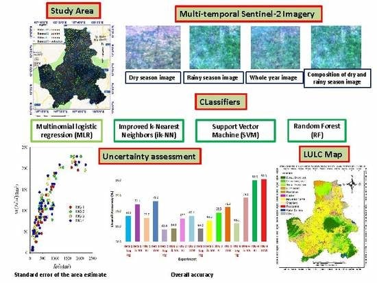
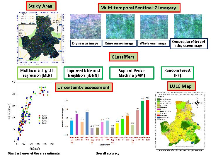
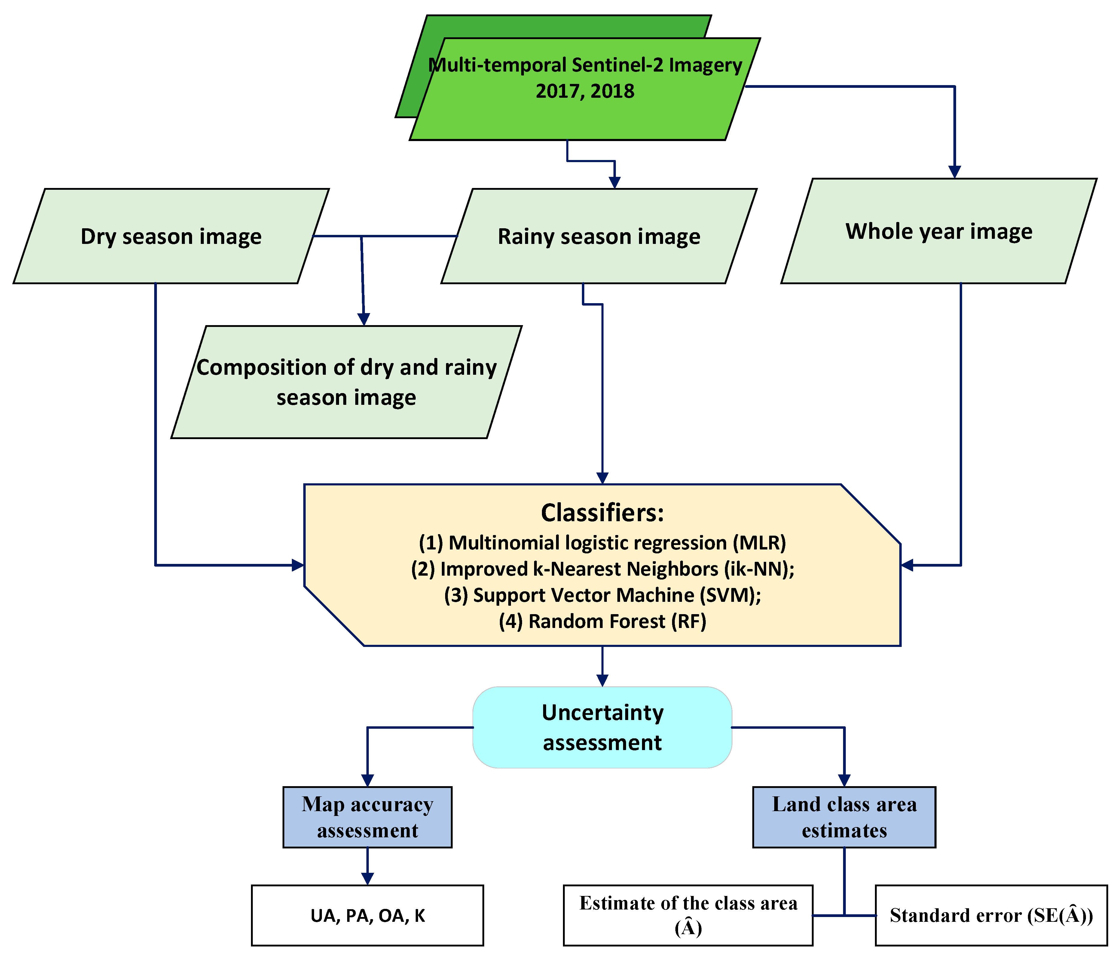
2.1. Overview
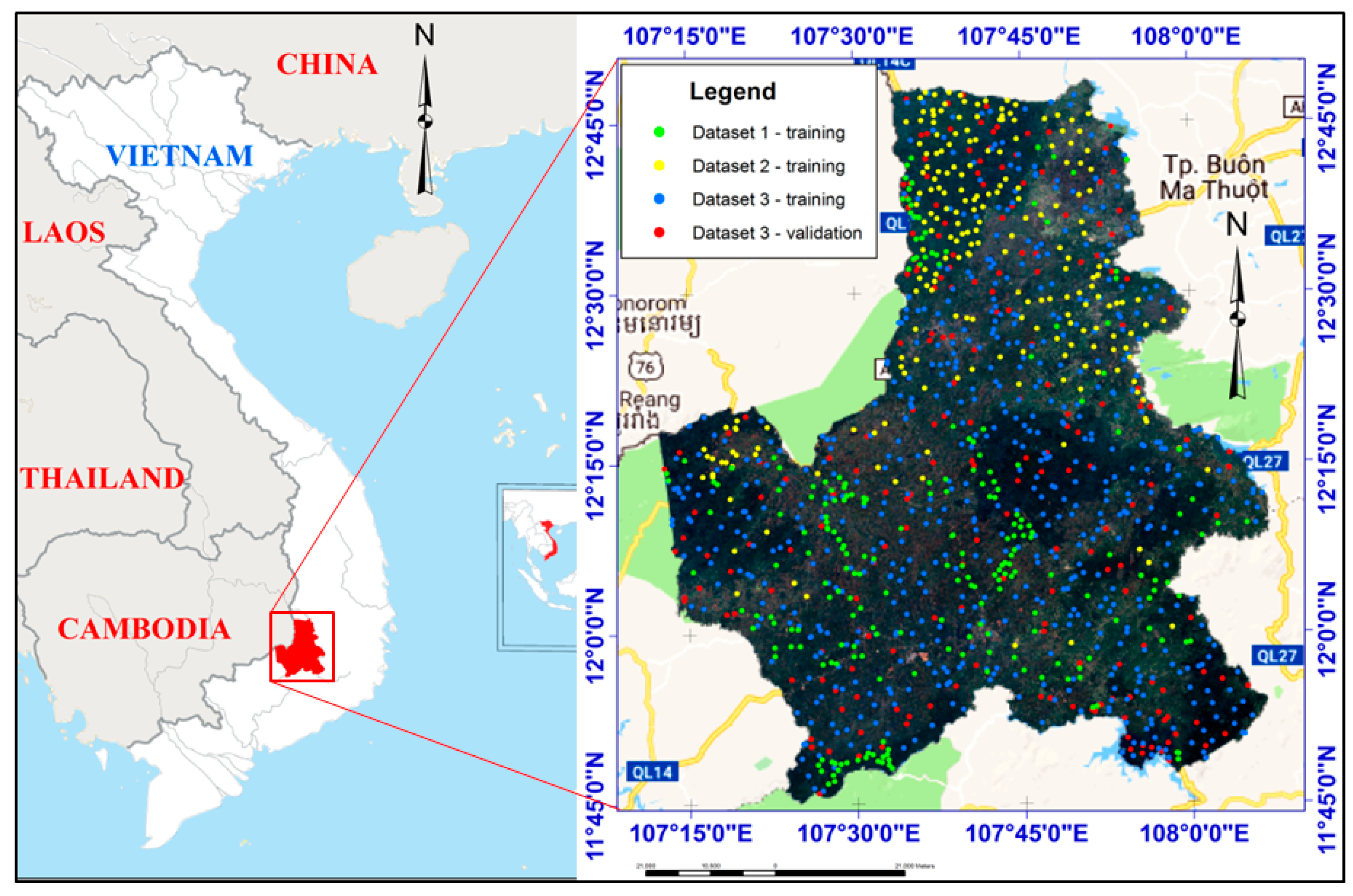
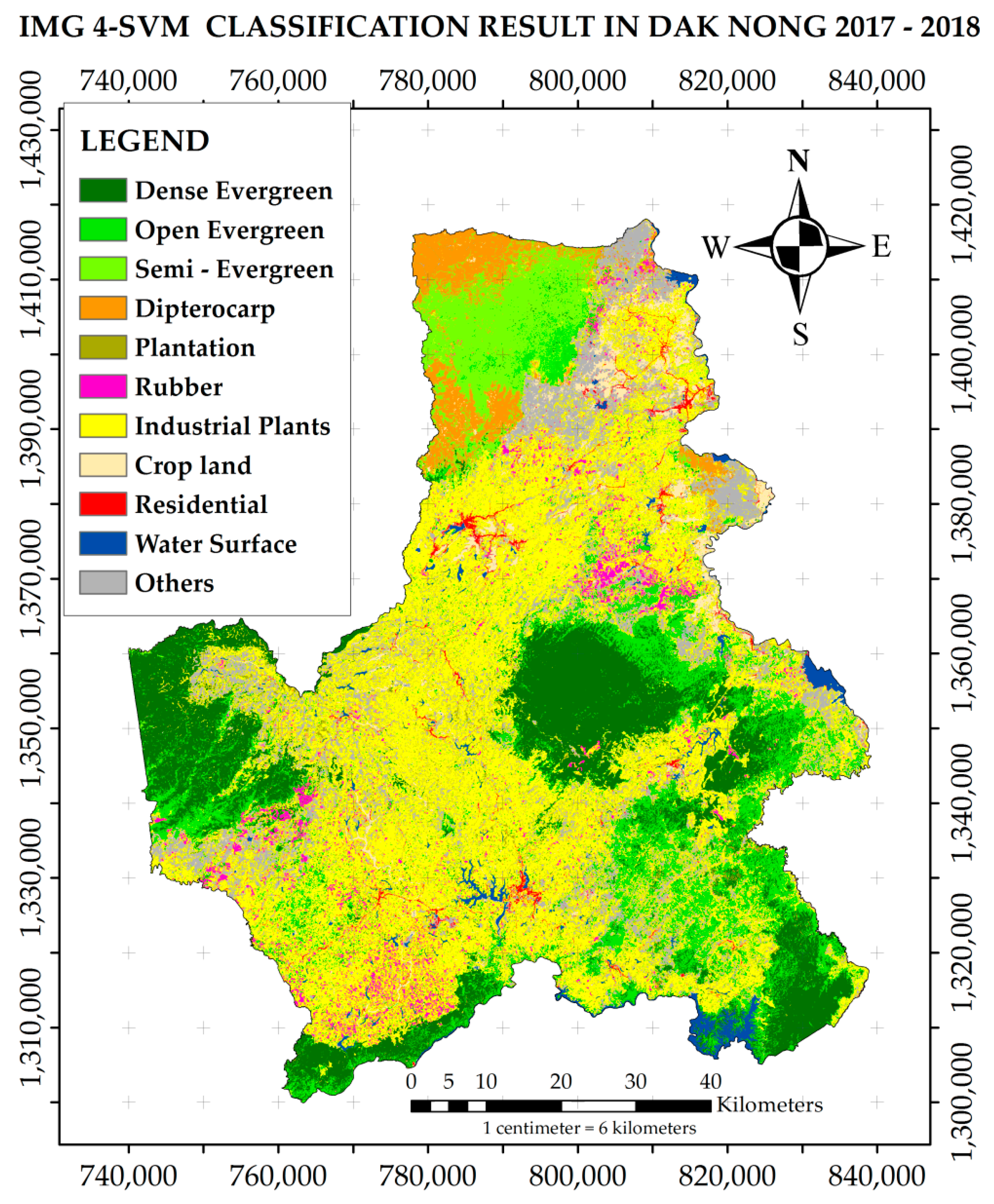
2.2. Study Area
2.3. Data
2.3.1. Sentinel-2 Imagery
2.3.2. Training and Validation Data
2.4. Classifiers
2.4.1. Multinomial Logistic Regression (MLR)
2.4.2. Improved k-Nearest Neighbors (ik-NN)
2.4.3. Support Vector Machine (SVM)
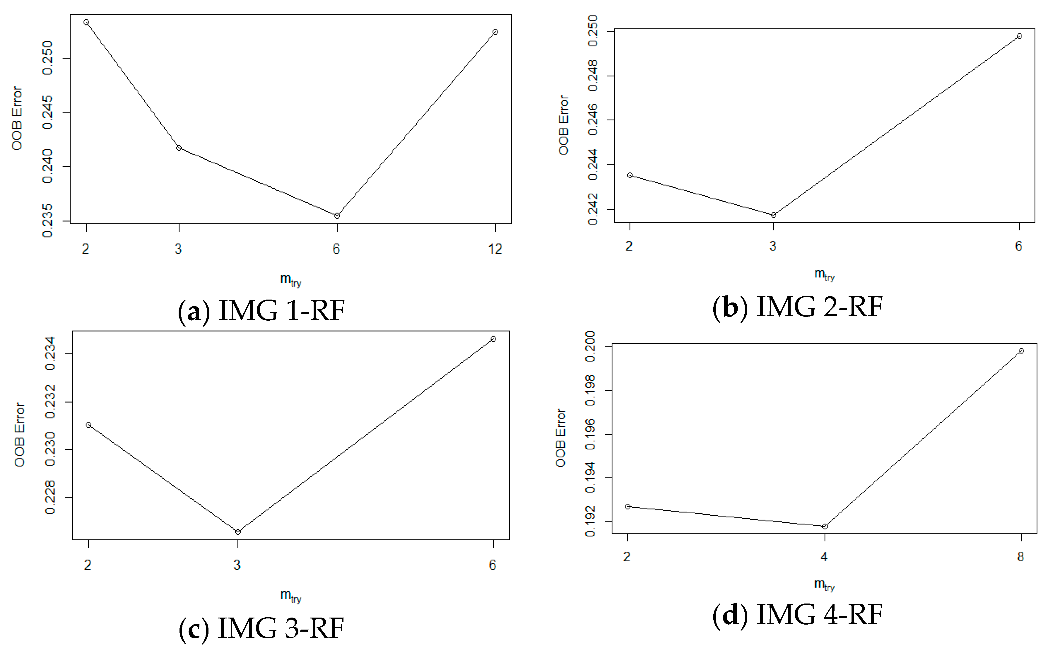
2.4.4. Random Forests (RF)
2.5. Analyses
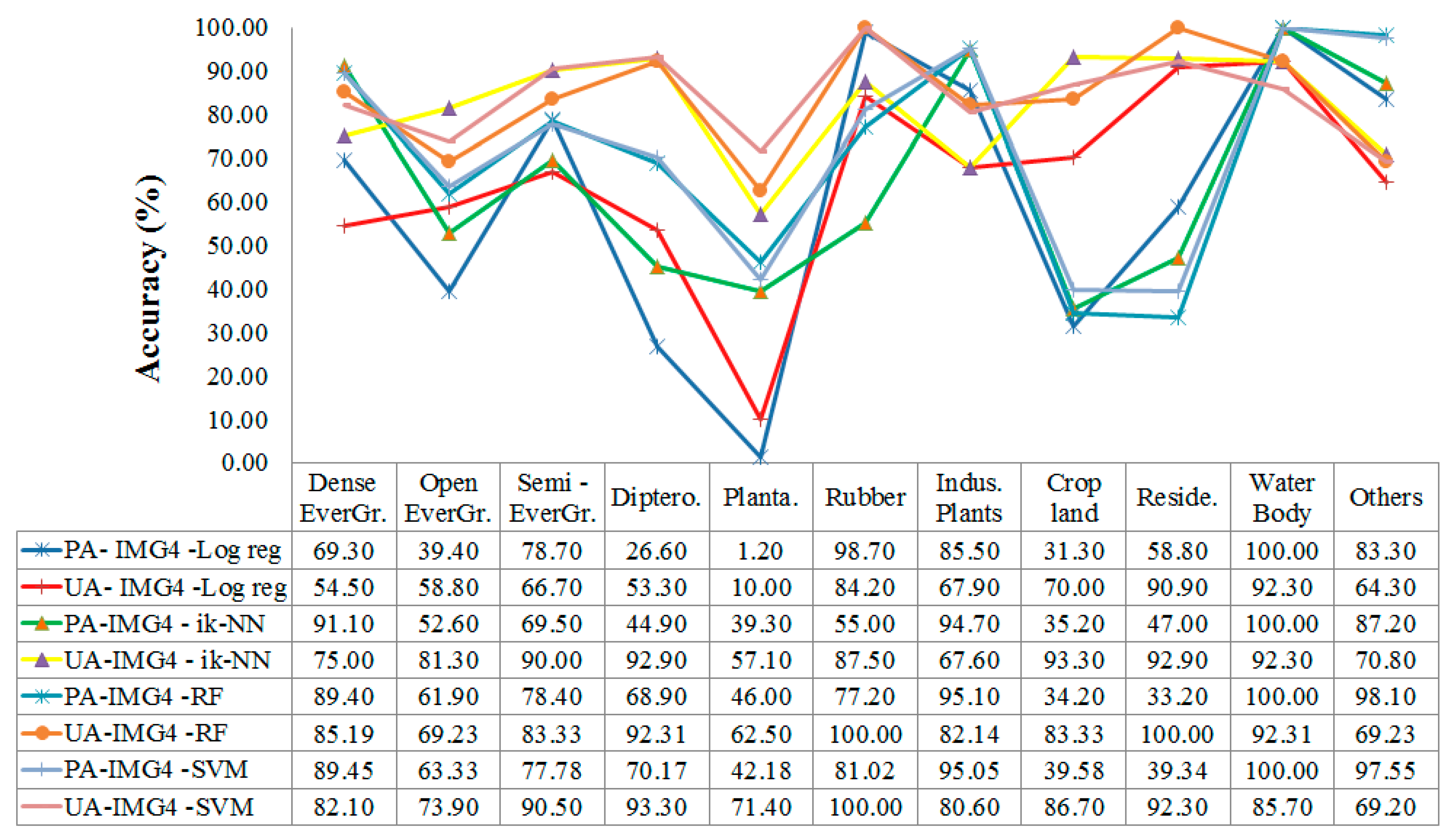
2.5.1. Accuracy Assessment
2.5.2. Land Cover Class Area Estimation
3. Results
3.1. Classifiers
3.1.1. Multinomial Logistic Regression (MLR)
3.1.2. Improved k-NN (ik-NN)
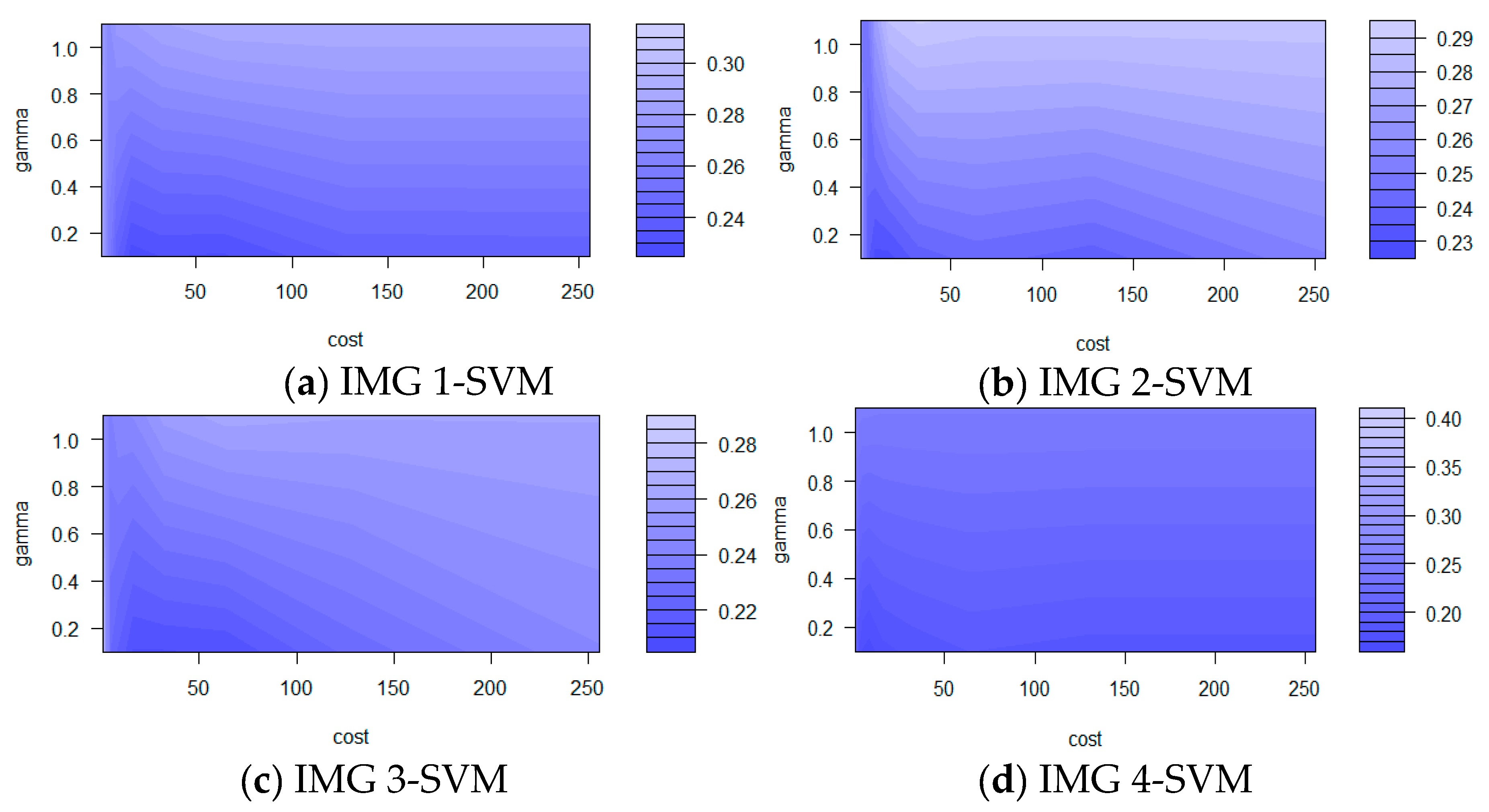
3.1.3. Support Vector Machine (SVM)
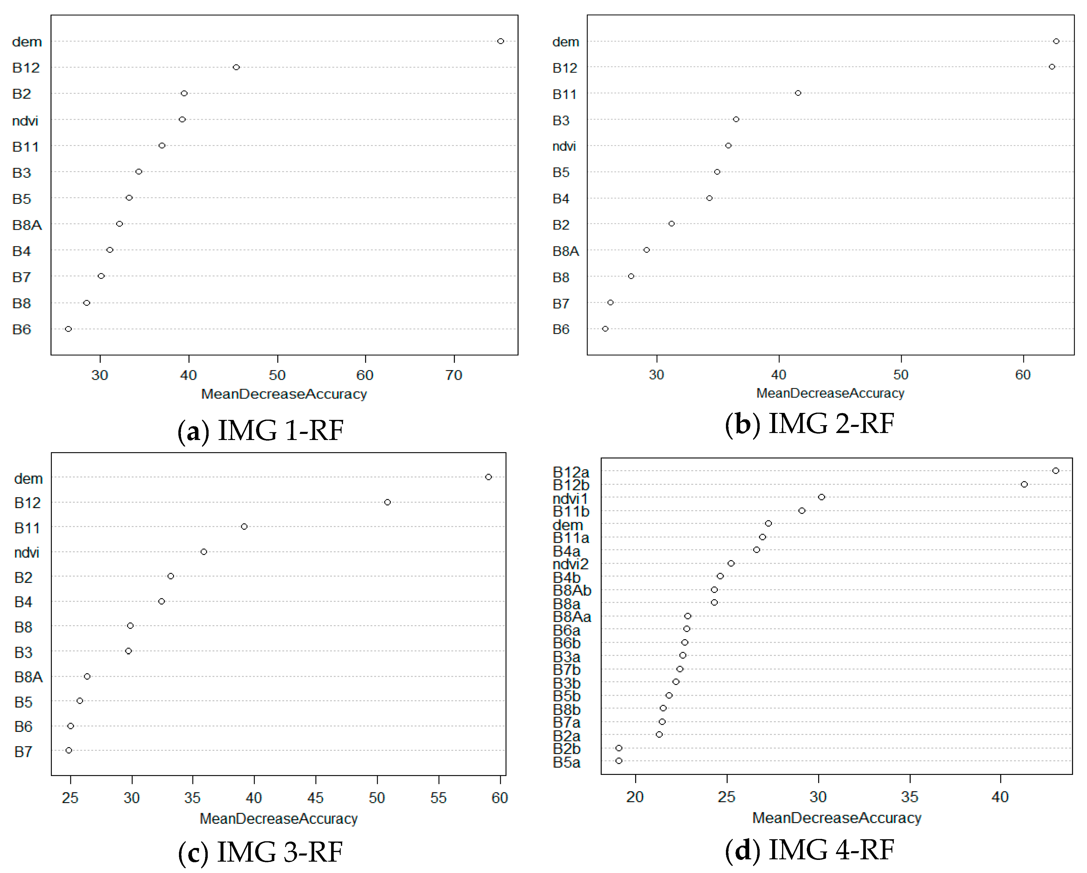
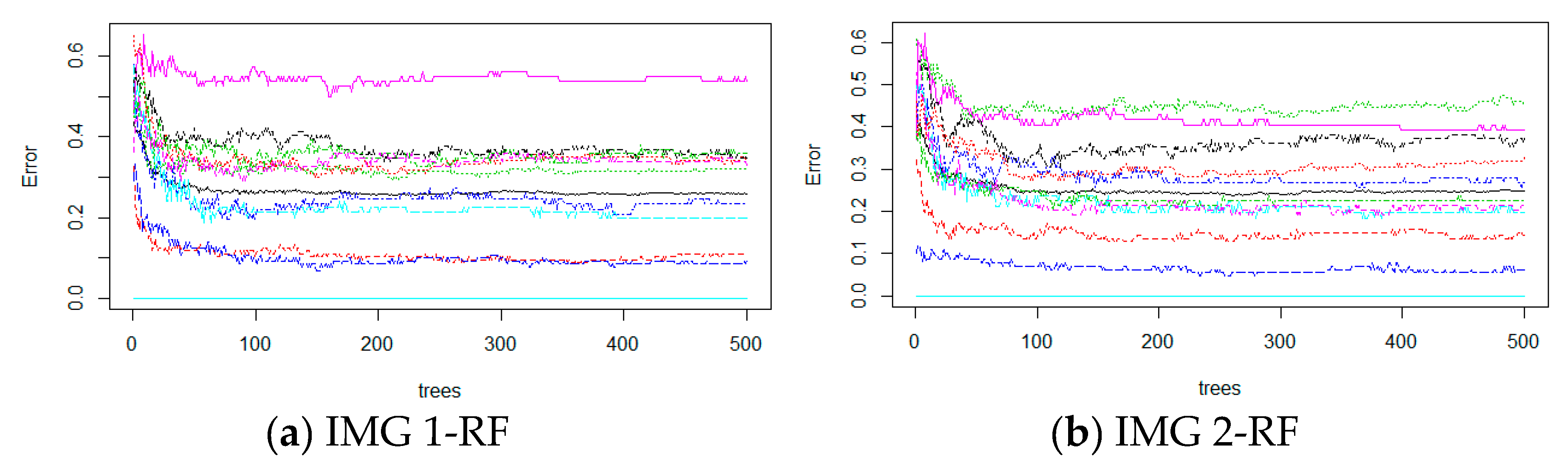
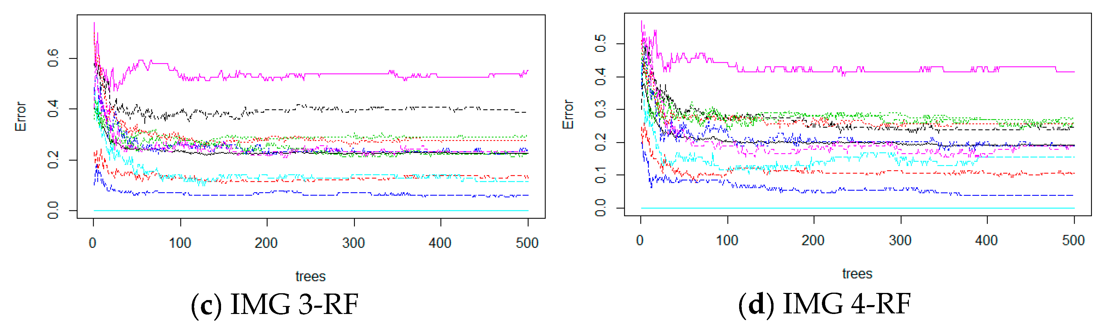
3.1.4. Random Forests (RF)
3.2. Analyses
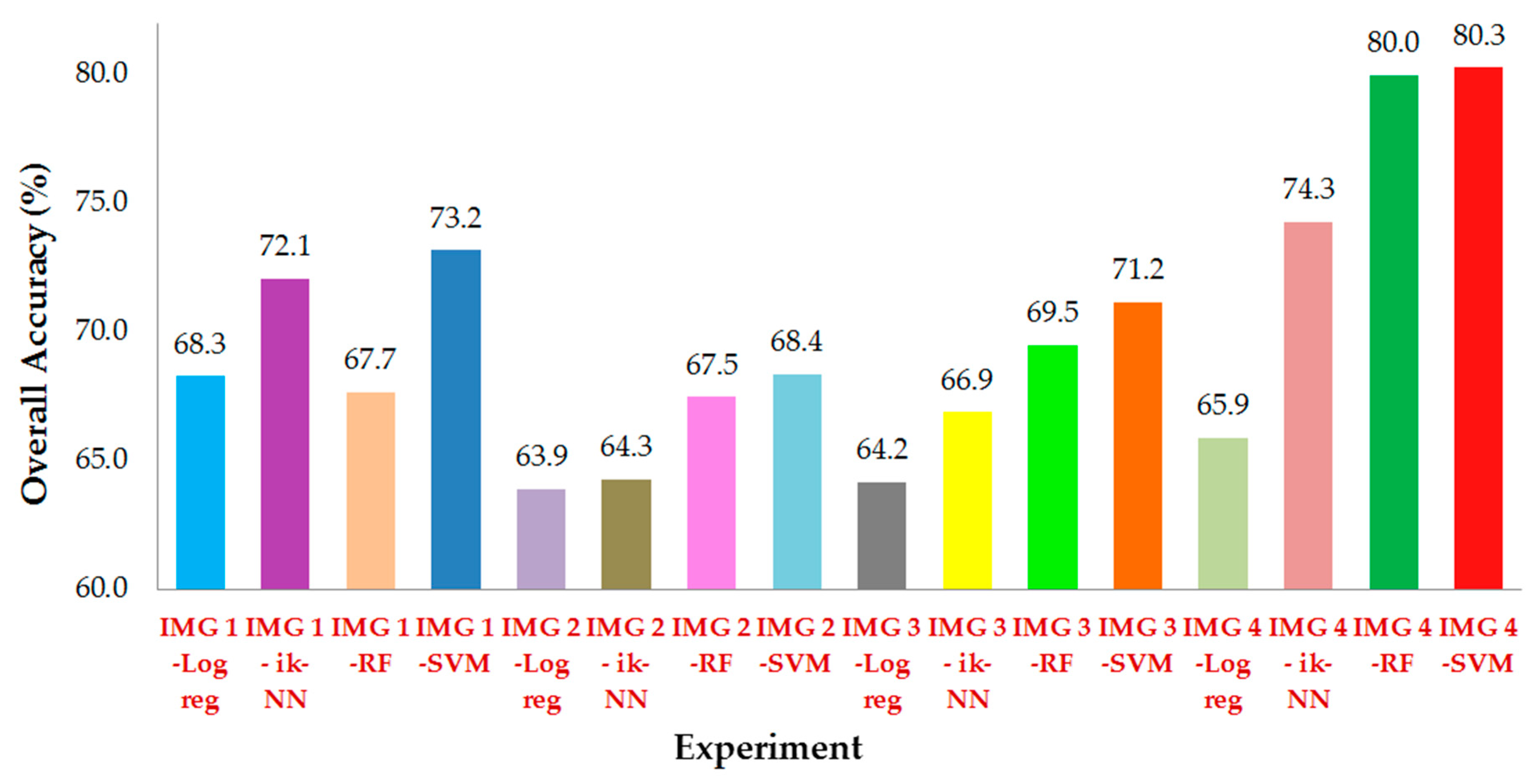
3.2.1. Accuracy of Classification Results
3.2.2. Land Cover Class Area Estimates
4. Discussion
5. Conclusions
Author Contributions
Funding
Acknowledgments
Conflicts of Interest
References
- Ministry of Agriculture and Rural Development. Decision on the Declaration of Forest Status of the Country in 2018; Decision No. 911/QD-BNN-LN; Ministry of Agriculture and Rural Development: Hanoi, Vietnam, 2019.
- Thai, V.T. Vietnamese Forest Vegetation, 1st ed.; Science and Technique Publishing House: Hanoi, Vietnam, 1978. [Google Scholar]
- Hoang, M.H.; Do, T.H.; van Noordwijk, M.; Pham, T.T.; Palm, M.; To, X.P.; Doan, D.; Nguyen, T.X.; Hoang, T.V.A. An Assessment of Opportunities for Reducing Emissions from All Land Uses–Vietnam Preparing for REDD. Final National Report; ASB Partnership for the Tropical Forest Margins: Nairobi, Kenya, 2010; p. 85. [Google Scholar]
- Burkhard, B.; Kroll, F.; Nedkov, S.; Müller, F. Mapping ecosystem service supply, demand and budgets. Ecol. Indic. 2012, 21, 17–29. [Google Scholar] [CrossRef]
- Gebhardt, S.; Wehrmann, T.; Ruiz, M.A.M.; Maeda, P.; Bishop, J.; Schramm, M.; Kopeinig, R.; Cartus, O.; Kellndorfer, J.; Ressl, R.; et al. MAD-MEX: Automatic wall-to-wall land cover monitoring for the Mexican REDD-MRV program using all Landsat data. Remote Sens. 2014, 6, 3923–3943. [Google Scholar] [CrossRef] [Green Version]
- Nguyen, T.T.H.; Doan, M.T.; Volker, R. Applying random forest classification to map land use/land cover using landsat 8 OLI. Int. Soc. Photogramm. Remote Sens. 2018, XLII-3/W4, 363–367. [Google Scholar] [CrossRef] [Green Version]
- Arnold, F.E.; van der Werf, N.; Rametsteiner, E. Strengthening Evidence-Based Forest Policy-Making: Linking Forest Monitoring With National Forest Programmes; Forestry Policy and Institutions Working; FAO: Rome, Italy, 2014; p. 33. [Google Scholar]
- Khatami, R.; Mountrakis, G.; Stehman, S.V. A meta-analysis of remote sensing research on supervised pixel-based land cover image classification processes: General guidelines for practitioners and future research. Remote Sens. Environ. 2016, 177, 89–100. [Google Scholar] [CrossRef] [Green Version]
- Jensen, J.R.; Cowen, D.C. Remote sensing of urban/suburban infrastructure and socioeconomic attributes. Photogramm. Eng. Remote Sens. 1999, 65, 611–622. [Google Scholar]
- Deka, J.; Tripathi, O.P.; Khan, M.L. Study on land use/land cover change dynamics through remote sensing and GIS–A case study of Kamrup District, North East India. J. Remote Sens. GIS 2014, 5, 55–62. [Google Scholar]
- Topaloğlu, H.R.; Sertel, E.; Musaoğlu, N. Assessment of classification accuracies of SENTINEL-2 and LANDSAT-8 data for land cover/use mapping. Int. Arch. Photogramm. Remote Sens. Spat. Inf. Sci. 2016, XLI-B8, 1055–1059. [Google Scholar]
- Gomez, C.; White, J.C.; Wulder, M.A. Optical remotely sensed time series data for land cover classification: A review. Int. Soc. Photogramm. 2016, 116, 55–72. [Google Scholar] [CrossRef] [Green Version]
- Sothe, C.; Almeida, C.M.; Liesenberg, V.; Schimalski, M.B. Evaluating sentinel-2 and landsat-8 data to map sucessional forest stages in a subtropical forest in Southern Brazil. Remote Sens. 2017, 9, 838. [Google Scholar] [CrossRef] [Green Version]
- Addabbo, P.; Focareta, M.; Marcuccio, S.; Votto, C.; Ullo, S.L. Contribution of sentinel-2 data for applications in vegetation monitoring. Acta IMEKO 2016, 5, 44–54. [Google Scholar] [CrossRef]
- Song, X.; Yang, C.; Wu, M.; Zhao, C.; Yang, G.; Hoffmann, W.C.; Huang, W. Evaluation of sentinel-2a satellite imagery for mapping cotton root rot. Remote Sens. 2017, 9, 906. [Google Scholar] [CrossRef] [Green Version]
- Li, J.; Roy, D.P. A global analysis of sentinel-2a, sentinel-2b and landsat-8 data revisit intervals and implications for terrestrial monitoring. Remote Sens. 2017, 9, 902. [Google Scholar]
- Pirotti, F.; Sunar, F.; Piragnolo, M. Benchmark of machine learning methods for classification of a sentinel-2 image. Int. Arch. Photogramm. Remote Sens. Spat. Inf. Sci. 2016, XLI-B7, 335–340. [Google Scholar] [CrossRef]
- Pelletier, C.; Valero, S.; Inglada, J.; Champion, N.; Dedieu, G. Assessing the robustness of Random Forests to map land cover with high resolution satellite image time series over large areas. Remote Sens. Environ. 2016, 187, 156–168. [Google Scholar] [CrossRef]
- Sharma, R.C.; Hara, K.; Tateishi, R. High-resolution vegetation mapping in japan by combining sentinel-2 and landsat 8 based multi-temporal datasets through machine learning and cross-validation approach. Land 2017, 6, 50. [Google Scholar] [CrossRef] [Green Version]
- Phan, T.N.; Kappas, M. Comparison of random forest, k-nearest neighbor, and support vector machine classifiers for land cover classification using sentinel-2 imagery. Sensors 2018, 18, 20. [Google Scholar]
- Nguyen, T.T.H. Forestry Remote Sensing: Multi-Source Data in Natural Evergreen Forest Inventory in the Central Highlands of Vietnam, 1st ed.; Lambert Academic Publishing: Saarbruecken, Germany, 2011; p. 165. [Google Scholar]
- Manandhar, R.; Odeh, I.O.A.; Ancev, T. Improving the accuracy of land use and land cover classification of landsat data using post-classification enhancement. Remote Sens. 2009, 1, 330–344. [Google Scholar] [CrossRef] [Green Version]
- Heydari, S.S.; Mountrakis, G. Effect of classifier selection, reference sample size, reference class distribution and scene heterogeneity in per-pixel classification accuracy using 26 Landsat sites. Remote Sens. Environ. 2018, 204, 648–658. [Google Scholar] [CrossRef]
- Lu, D.; Weng, Q.A. Survey of image classification methods and techniques for improving classification performance. Int. J. Remote Sens. 2007, 28, 823–870. [Google Scholar] [CrossRef]
- Waske, B.; Braun, M. Classifier ensembles for land cover mapping using multitemporal SAR imagery. ISPRS J. Photogramm. Remote Sens. 2009, 64, 450–457. [Google Scholar] [CrossRef]
- Li, C.; Wang, J.; Wang, L.; Hu, L.; Gong, P. Comparison of classification algorithms and training sample sizes in urban land classification with Landsat Thematic Mapper imagery. Remote Sens. 2014, 6, 964–983. [Google Scholar] [CrossRef] [Green Version]
- Abbas, A.W.; Minallh, N.; Ahmad, N.; Abid, S.A.R.; Khan, M.A.A. K-means and ISODATA clustering algorithms for landcover classification using remote sensing. Sindh Univ. Res. J. (Sci. Ser.) 2016, 48, 315–318. [Google Scholar]
- Paola, J.D.; Schowengerdt, R.A. A detailed comparison of backpropagation neural network and maximum-likelihood classifiers for urban land use classification. IEEE Trans. Geosci. Remote Sens. 1995, 33, 981–996. [Google Scholar] [CrossRef]
- Shafri, H.Z.M.; Suhaili, A.; Mansor, S. The performance of maximum likelihood, spectral angle mapper, neural network and decision tree classifiers in hyperspectral image analysis. J. Comput. Sci. 2007, 3, 419–423. [Google Scholar] [CrossRef] [Green Version]
- Santos, J.A.; Ferreira, C.D.; Torres, R.D.S.; Gonalves, M.A.; Lamparelli, R.A.C. A relevance feedback method based on genetic programming for classification of remote sensing images. Inf. Sci. 2011, 181, 2671–2684. [Google Scholar] [CrossRef]
- Ahmad, A.; Quegan, S. Analysis of maximum likelihood classification on multispectral data. Appl. Math. Sci. 2012, 6, 6425–6436. [Google Scholar]
- McRoberts, R.E. A two-step nearest neighbors algorithm using satellite imagery for predicting forest structure within species composition classes. Remote Sens. Environ. 2009, 113, 532–545. [Google Scholar] [CrossRef]
- McRoberts, R.E. Satellite image-based maps: Scientific inference or pretty pictures? Remote Sens. Environ. 2011, 115, 714–724. [Google Scholar] [CrossRef]
- Pal, M.; Mather, P.M. Support vector classifiers for land cover classification. In Proceedings of the Map India Conference, New Delhi, India, 28–31 January 2003. [Google Scholar]
- Huang, C.; Davis, L.S.; Townshend, J.R.G. An assessment of support vector machines for land cover classification. Int. J. Remote Sens. 2002, 23, 725–749. [Google Scholar] [CrossRef]
- Bahari, N.I.S.; Ahmad, A.; Aboobaider, B.M. Application of support vector machine for classification of multispectral data. IOP Conf. Ser. Earth Environ. Sci. 2014, 20. [Google Scholar] [CrossRef]
- Balcik, F.B.; Kuzucu, A.K. Determination of land cover/land use using spot 7 data with supervised classification methods. Int. Arch. Photogramm. Remote Sens. Spat. Inf. Sci. 2016, XLII-2/W1, 143–146. [Google Scholar] [CrossRef] [Green Version]
- Franco-Lopez, H.; Ek, A.R.; Bauer, M.E. Estimation and mapping of forest stand density, volume, and cover type using the k-nearest neighbors method. Remote Sens. Environ. 2001, 77, 251–274. [Google Scholar] [CrossRef]
- Yu, S.; Backer, S.; Scheunders, P. Genetic feature selection combined with composite fuzzy nearest neighbor classifiers for hyperspectral satellite imagery. Pattern Recognit. Lett. 2002, 23, 183–190. [Google Scholar] [CrossRef]
- Lowe, B.; Kulkarni, A. Multispectral image analysis using random forest. Int. J. Soft Comput. (IJSC) 2015, 6, 14. [Google Scholar] [CrossRef]
- Kennedy, R.E.; Yang, Z.; Braaten, J.; Copass, C.; Antonova, N.; Jordan, C.; Nelson, P. Attribution of disturbance change agent from Landsat time-series in support of habitat monitoring in the Puget Sound region, USA. Remote Sens. Environ. 2015, 166, 271–285. [Google Scholar] [CrossRef]
- Basten, K. Classifying Landsat Terrain Images via Random Forests. Bachelor thesis Computer Science; Radboud University: Nijmegen, The Netherlands, 2016. [Google Scholar]
- Naidoo, L.; Cho, M.A.; Mathieu, R.; Asner, G. Classification of savanna tree species, in the Greater Kruger National Park region, by integrating hyperspectral and LiDAR data in a random forest data mining environment. ISPRS J. Photogramm. Remote Sens. 2012, 69, 167–179. [Google Scholar] [CrossRef]
- Tomppo, E.; Halme, M. Using coarse scale forest variables as ancillary information and weighting of variables in k-NN estimation: A genetic algorithm approach. Remote Sens. Environ. 2004, 92, 1–20. [Google Scholar] [CrossRef]
- Tomppo, E.; Gagliano, C.; De Natale, F.; Katila, M.; McRoberts, R. Predicting categorical forest variables using an improved k-nearest neighbor estimator and Landsat imagery. Remote Sens. Environ. 2009, 113, 500–517. [Google Scholar] [CrossRef]
- Dharamvir. Object oriented model classification of satellite image. CDQM 2013, 16, 46–54. [Google Scholar]
- Machala, M.; Zejdová, L. Forest mapping through object-based image analysis of multispectral and lidar aerial data. Eur. J. Remote Sens. 2014, 47, 117–131. [Google Scholar] [CrossRef]
- Mora, A.; Santos, T.M.A.; Łukasik, S.; Silva, J.M.N.; Falcão, A.J.; Fonseca, J.M.; Ribeiro, R.A. Land cover classification from multispectral data using computational intelligence tools: A comparative study. Information 2017, 8, 147. [Google Scholar] [CrossRef] [Green Version]
- Sowmya, B.; Sheelarani, B. Land cover classification using reformed fuzzy C-means. Sadhana 2011, 36, 153–165. [Google Scholar] [CrossRef]
- Apte, K.S.; Patravali, D.S. Development of back propagation neutral network model for ectracting the feature from a satellite image using curvelet transform. Int. J. Eng. Res. Gen. Sci. 2015, 3, 226–236. [Google Scholar]
- Ma, L.; Li, M.; Ma, X.; Cheng, L.; Du, P.; Liu, Y. A review of supervised object-based land-cover image classification. ISPRS J. Photogramm. Remote Sens. 2017, 130, 277–293. [Google Scholar] [CrossRef]
- Meyfroidt, P.; Lambin, E.F.; Erb, K.H.; Hertel, T.W. Globalization of land use: Distant drivers of land change and geographic displacement of land use. Curr. Opin. Environ. Sustain. 2013, 5, 438–444. [Google Scholar] [CrossRef]
- Bourgoin, C.; Oszwald, J.; Bourgoin, J.; Gond, V.; Blanc, L.; Dessard, H.; Phan, T.V.; Sist, P.; Läderach, P.; Reymondin, L.; et al. Assessing the ecological vulnerability of forest landscape to agricultural frontier expansion in the Central Highlands of Vietnam. Int. J. Appl. Earth Obs. Geoinf. 2020, 84, 13. [Google Scholar] [CrossRef]
- Ha, T.V.; Tuohy, M.; Irwin, M.; Tuan, P.T. Monitoring and mapping rural urbanization and land use changes using Landsat data in the northeast subtropical region of Vietnam. Egypt. J. Remote Sens. Space Sci. 2020, 23, 11–19. [Google Scholar] [CrossRef]
- Drusch, M.; Del Bello, U.; Carlier, S.; Colin, O.; Fernandez, V.; Gascon, F.; Hoersch, B.; Isola, C.; Laberinti, P.; Martimort, P.; et al. Sentinel-2: ESA’s optical high-resolution mission for GMES operational services. Remote Sens. Environ. 2012, 120, 25–36. [Google Scholar] [CrossRef]
- Vuolo, F.; Zółtak, M.; Pipitone, C.; Zappa, L.; Wenng, H.; Immitzer, M.; Weiss, M.; Baret, F.; Atzberger, C. Data service platform for Sentinel-2 surface reflectance and value-added products: System use and examples. Remote Sens. 2016, 8, 938. [Google Scholar] [CrossRef] [Green Version]
- Yacouba, D.; Guangdao, H.; Xingping, W. Assessment of land use cover changes using NDVI and DEM in Puer and Simao Counties, Yunnan Province, China. World Rural Obs. 2009, 1, 1–11. [Google Scholar]
- Defries, R.S.; Townshend, J.R.G. NDVI-derived land cover classifications at a global scale. Int. J. Remote Sens. 1994, 15, 3567–3586. [Google Scholar] [CrossRef]
- Pettorelli, N.; Ryan, S.; Mueller, T.; Bunnefeld, N.; Jedrzejewska, B.; Lima, M.; Kausrud, K. The Normalized Difference Vegetation Index (NDVI): Unforeseen successes in animal ecology. Clim. Res. 2011, 46, 15–27. [Google Scholar] [CrossRef]
- Housman, I.W.; Chastain, R.A.; Finco, M.V. An evaluation of forest health insect and disease survey data and satellite-based remote sensing forest change detection methods: Case studies in the United States. Remote Sens. 2018, 10, 21. [Google Scholar] [CrossRef] [Green Version]
- Gorelick, N.; Hancher, M.; Dixon, M.; Ilyushchenko, S.; Thau, D.; Moore, R. Google earth engine: Planetary-scale geospatial analysis for everyone. Remote. Sens. Environ. 2017, 202, 18–27. [Google Scholar] [CrossRef]
- Housman, I.; Hancher, M.; Stam, C. A quantitative evaluation of cloud and cloud shadow masking algorithms available in Google Earth Engine. Manuscript in preparation. Unpublished work.
- Roy, D.P.; Li, Z.; Zhang, H.K. Adjustment of sentinel-2 multi-spectral instrument (msi) red-edge band reflectance to nadir BRDF adjusted reflectance (NBAR) and quantification of red-edge band BRDF effects. Remote Sens. 2017, 9, 1325. [Google Scholar]
- Roy, D.P.; Li, J.; Zhang, H.K.; Yan, L.; Huang, H. Examination of sentinel-2A multi-spectral instrument (MSI) reflectance anisotropy and the suitability of a general method to normalize MSI reflectance to nadir BRDF adjusted reflectance. Remote Sens. Environ. 2017, 199, 25–38. [Google Scholar] [CrossRef]
- Soenen, S.A.; Peddle, D.R.; Coburn, C.A. SCS+ C: A modified sun-canopy-sensor topographic correction in forested terrain. IEEE Trans. Geosci. Remote Sens. 2005, 43, 2148–2159. [Google Scholar] [CrossRef]
- Google Earth Engine. Developer’s Guide. ImageCollection Reductions. Available online: https://developers.google.com/earth-engine/reducers_image_collection (accessed on 29 October 2017).
- De Alban, J.D.T.; Connette, G.M.; Oswald, P.; Webb, E.L. Combined landsat and L-band SAR data improves land cover classification and change detection in dynamic tropical landscapes. Remote Sens. 2018, 10, 306. [Google Scholar] [CrossRef] [Green Version]
- Gilat, D.; Hill, T.P. Quantile-locating functions and the distance between the mean and quantiles. Stat. Neerl. 1993, 47, 279–283. [Google Scholar] [CrossRef] [Green Version]
- Google Earth Engine. Developer’s Guide. Scale. Available online: https://developers.google.com/earth-engine/scale#scale-of-analysis (accessed on 29 October 2017).
- Open Geo Blog–Tutorials, Code Snippets and Examples to Handle Spatial Data. Available online: https://mygeoblog.com/ (accessed on 28 October 2018).
- Teluguntla, P.; Thenkabail, P.S.; Oliphant, A.; Xiong, J.; Gumma, M.K.; Congalton, R.G.; Kamini Yadav, K.; Huete, A. A 30-m landsat-derived cropland extent product of Australia and China using random forest machine learning algorithm on Google Earth Engine cloud computing platform. ISPRS J. Photogramm. Remote Sens. 2018, 144, 325–340. [Google Scholar] [CrossRef]
- Särndal, C.-E.; Swensson, B.; Wretman, J. Model Assisted Survey Sampling; Springer: New York, NY, USA, 1992. [Google Scholar]
- Chirici, G.; Mura, M.; McInerney, D.; Py, N.; Tomppo, E.O.; Waser, L.T.; McRoberts, R.E. A meta-analysis and review of the literature on the k-Nearest Neighbors technique for forestry applications that use remotely sensed data. Remote Sens. Environ. 2016, 176, 282–294. [Google Scholar] [CrossRef]
- McRoberts, R.E.; Domke, G.M.; Chen, Q.; Næsset, E.; Gobakken, T. Using genetic algorithms to optimize k-Nearest Neighbors configurations for use with airborne laser scanning data. Remote Sens. Environ. 2016, 184, 387–395. [Google Scholar] [CrossRef]
- Cortes, C.; Vapnik, V. Support-vector networks. Mach. Learn. 1995, 20, 273–297. [Google Scholar] [CrossRef]
- Meyer, D.; Leisch, F.; Hornik, K. Benchmarking Support Vector Machines; Report Series No. 78; Vienna University of Economics and Business Administration Augasse 2–6, 1090: Wien, Austria, 2002. [Google Scholar]
- Knorn, J.; Rabe, A.; Radeloff, V.C.; Kuemmerle, T.; Kozak, J.; Hostert, P. Land cover mapping of large areas using chain classification of neighboring Landsat satellite images. Remote. Sens. Environ. 2009, 113, 957–964. [Google Scholar] [CrossRef]
- Breiman, L. Random forests. Mach. Learn. 2001, 45, 5–32. [Google Scholar] [CrossRef] [Green Version]
- Liaw, A.; Wiener, M. Classification and regression by randomForest. R News 2002, 2, 18–22. [Google Scholar]
- Congalton, R.G.; Green, K. Assessing the Accuracy of Remotely Sensed Data: Principles and Practices; Lewis Publishers: Boca Raton, FL, USA, 1999. [Google Scholar]
- Cochran, W.G. Sampling Techniques, 3rd ed.; Wiley: New York, NY, USA, 1977. [Google Scholar]
- Olofsson, P.; Foody, G.M.; Herold, M.; Stehman, S.V.; Woodcock, C.E.; Wulder, M.A. Good practices for estimating area and assessing accuracy of land change. Remote Sens. Environ. 2014, 148, 42–57. [Google Scholar] [CrossRef]
- R Core Team. R: A Language and Environment for Statistical Computing; R Foundation for Statistical Computing: Vienna, Austria, 2019; Available online: https://www.R-project.org/ (accessed on 23 March 2020).
- Qian, Y.; Zhou, W.; Yan, J.; Li, W.; Han, L. Comparing machine learning classifiers for object-based land cover classification using very high resolution imagery. Remote Sens. 2015, 7, 153–168. [Google Scholar] [CrossRef]
- Sutter, J.M.; Kalivas, J.H. Comparison of forward selection, backward elimination, and generalized simulated annealing for variable selection. Micro. J. 1993, 47, 60–66. [Google Scholar] [CrossRef]
- Brown, J.F.; Loveland, T.R.; Ohlen, D.O.; Zhu, Z. The global land-cover characteristics database: The user’s perspective. Photogramm. Eng. Remote Sens. 1999, 65, 1069–1074. [Google Scholar]
- Lark, R.M. Components of accuracy of maps with special reference to discriminant analysis on remote sensor data. Int. J. Remote Sens. 1995, 16, 1461–1480. [Google Scholar] [CrossRef]
- Salovaara, K.J.; Thessler, S.; Malik, R.N.; Tuomisto, H. Classification of Amazonian primary rain forest vegetation using Landsat ETM+ satellite imagery. Remote Sens. Environ. 2005, 97, 39–51. [Google Scholar] [CrossRef]
- Foody, G.M. Status of land cover classification accuracy assessment. Remote Sens. Environ. 2002, 80, 185–201. [Google Scholar] [CrossRef]
- Anderson, J.R.; Hardy, E.E.; Roach, J.T.; Witmer, R.E. A Land Use and Land Cover Classification System for Use with Remote Sensor Data; U.S. Government Publishing Office: Washington, DC, USA, 1976.
- Foody, G.M. Harshness in image classification accuracy assessment. Int. J. Remote Sens. 2008, 29, 3137–3158. [Google Scholar] [CrossRef] [Green Version]
- Tomppo, E.; Katila, M.; Makisara, K.; Perasaari, J. Multi-source National Forest Inventory: Methods and applications; Springer: Dordrecht, The Netherlands, 2008. [Google Scholar]
- Xie, Z.; Chen, Y.; Lu, D.; Li, G.; Chen, E. Classification of land cover, forest, and tree species classes with ziyuan-3 multispectral and stereo data. Remote Sens. 2019, 11, 164. [Google Scholar] [CrossRef] [Green Version]


| Name | Min | Max | Scale | Resolution | Wavelength | Description |
|---|---|---|---|---|---|---|
| B1 | 0 | 10,000 | 0.0001 | 60 Meters | 443 nm | Aerosols |
| B2 | 0 | 10,000 | 0.0001 | 10 Meters | 490 nm | Blue |
| B3 | 0 | 10,000 | 0.0001 | 10 Meters | 560 nm | Green |
| B4 | 0 | 10,000 | 0.0001 | 10 Meters | 665 nm | Red |
| B5 | 0 | 10,000 | 0.0001 | 20 Meters | 705 nm | Red Edge 1 |
| B6 | 0 | 10,000 | 0.0001 | 20 Meters | 740 nm | Red Edge 2 |
| B7 | 0 | 10,000 | 0.0001 | 20 Meters | 783 nm | Red Edge 3 |
| B8 | 0 | 10,000 | 0.0001 | 10 Meters | 842 nm | Near infrared (NIR) |
| B8a | 0 | 10,000 | 0.0001 | 20 Meters | 865 nm | Red Edge 4 |
| B9 | 0 | 10,000 | 0.0001 | 60 Meters | 940 nm | Water vapor |
| B10 | 0 | 10,000 | 0.0001 | 60 Meters | 1375 nm | Cirrus |
| B11 | 0 | 10,000 | 0.0001 | 20 Meters | 1610 nm | Short-wave infrared (SWIR) 1 |
| B12 | 0 | 10,000 | 0.0001 | 20 Meters | 2190 nm | SWIR 2 |
| QA10 | 10 Meters | Always empty | ||||
| QA20 | 20 Meters | Always empty | ||||
| QA60 | 60 Meters | Cloud mask |
| Image Name | Time | Acquisition Date | Number of Images Involved | Number of Bands |
|---|---|---|---|---|
| IMG 1 | Dry season, 2017–2018 | 01/01/2017–03/31/2017 and 12/01/2017–03/31/2018 | 169 | 10 |
| IMG 2 | Rainy season, 2017–2018 | 04/01/2017–11/30/2017 and 04/01/2018–06/30/2018 | 277 | 10 |
| IMG 3 | All for year 2017 | 01/01/2017–12/31/2017 | 265 | 10 |
| IMG 4 | Combination of all bands for both 2017 and 2018 (IMG 1 + IMG 2) | Dry season 2017–2018 + Rainy season 2017–2018 | 446 | 20 |
| Dataset | Use | Land Cover Class | Total | ||||||||||
|---|---|---|---|---|---|---|---|---|---|---|---|---|---|
| 1 | 2 | 3 | 4 | 5 | 6 | 7 | 8 | 9 | 10 | 11 | |||
| 1 | Training | 77 | 6 | 15 | 13 | 29 | 34 | 0 | 13 | 32 | 4 | 9 | 232 |
| 2 | Training | 6 | 8 | 52 | 33 | 11 | 14 | 19 | 21 | 20 | 4 | 25 | 213 |
| 3 | Training | 99 | 97 | 22 | 9 | 0 | 17 | 234 | 20 | 8 | 11 | 74 | 591 |
| Total | Training | 182 | 111 | 89 | 55 | 40 | 65 | 253 | 54 | 60 | 19 | 108 | 1036 |
| 3 | Validation | 25 | 25 | 22 | 17 | 7 | 17 | 28 | 20 | 16 | 12 | 19 | 208 |
| Classification Algorithm | Image Set | Number of Bands |
|---|---|---|
| ik-NN | IMG 1 | 10 |
| IMG 2 | 10 | |
| IMG 3 | 10 | |
| IMG 4 | 20 | |
| MLR | IMG 1 | 10 |
| IMG 2 | 10 | |
| IMG 3 | 10 | |
| IMG 4 | 20 | |
| SVM | IMG 1 | 10 |
| IMG 2 | 10 | |
| IMG 3 | 10 | |
| IMG 4 | 20 | |
| RF | IMG 1 | 10 |
| IMG 2 | 10 | |
| IMG 3 | 10 | |
| IMG 4 | 20 |
| Map Class | Reference Class | Total | UA * | |||
|---|---|---|---|---|---|---|
| C | ~C | |||||
| C | ||||||
| ~C | ||||||
| Total | ||||||
| PA * | ||||||
| Image | Classifier | OA | Kappa | Accuracy | Land Class * | ||||||||||
|---|---|---|---|---|---|---|---|---|---|---|---|---|---|---|---|
| 1 | 2 | 3 | 4 | 5 | 6 | 7 | 8 | 9 | 10 | 11 | |||||
| IMG 1 | MLR | 68.3 | 0.657 | PA | 97.60 | 35.50 | 70.00 | 39.40 | 0.000 | 47.70 | 91.40 | 47.10 | 48.60 | 100.00 | 89.30 |
| UA | 58.50 | 66.70 | 66.70 | 80.00 | 0.000 | 68.80 | 75.90 | 70.00 | 100.00 | 85.70 | 61.50 | ||||
| 821.72 | 932.59 | 502.16 | 378.25 | 241.3 | 456.51 | 1923.88 | 502.16 | 202.17 | 91.3 | 469.56 | |||||
| 104.35 | 156.52 | 97.82 | 97.82 | 84.78 | 110.87 | 195.65 | 123.91 | 45.65 | 13.04 | 71.74 | |||||
| Ik-NN | 72.1 | 0.732 | PA | 98.20 | 55.40 | 81.90 | 45.10 | 32.50 | 38.30 | 93.60 | 28.20 | 31.60 | 100.00 | 87.70 | |
| UA | 80.00 | 65.20 | 80.80 | 80.00 | 60.00 | 84.60 | 68.60 | 91.70 | 91.70 | 92.30 | 62.10 | ||||
| 886.94 | 808.68 | 404.34 | 541.29 | 202.17 | 463.04 | 1878.23 | 456.51 | 189.13 | 97.82 | 593.47 | |||||
| 78.26 | 143.48 | 78.26 | 123.91 | 71.74 | 130.43 | 208.69 | 123.91 | 52.17 | 6.52 | 104.35 | |||||
| RF | 67.7 | 0.67 | PA | 92.20 | 64.00 | 62.10 | 42.10 | 46.90 | 18.90 | 89.90 | 38.40 | 42.00 | 100.00 | 87.80 | |
| UA | 77.40 | 63.00 | 85.70 | 81.80 | 66.70 | 100.00 | 59.50 | 85.70 | 91.70 | 92.30 | 58.10 | ||||
| 886.94 | 763.03 | 502.16 | 515.21 | 182.61 | 697.81 | 1689.10 | 397.82 | 215.21 | 104.35 | 567.38 | |||||
| 104.35 | 123.91 | 104.35 | 123.91 | 58.69 | 163.04 | 215.21 | 97.82 | 52.17 | 6.52 | 104.35 | |||||
| SVM | 73.2 | 0.748 | PA | 94.90 | 54.30 | 73.60 | 47.10 | 26.80 | 36.20 | 94.40 | 42.80 | 46.50 | 100.00 | 84.80 | |
| UA | 76.70 | 64.00 | 87.00 | 100.00 | 60.00 | 78.60 | 70.60 | 92.30 | 92.90 | 92.30 | 63.00 | ||||
| 880.42 | 886.94 | 404.34 | 456.51 | 189.13 | 397.82 | 1956.49 | 463.04 | 169.56 | 104.35 | 613.03 | |||||
| 91.3 | 163.04 | 84.78 | 110.87 | 71.74 | 117.39 | 215.21 | 104.35 | 52.17 | 6.52 | 110.87 | |||||
| IMG 2 | MLR | 63.9 | 0.611 | PA | 67.80 | 37.70 | 71.80 | 33.70 | 8.80 | 96.30 | 85.30 | 39.50 | 41.40 | 100.00 | 86.20 |
| UA | 54.50 | 58.80 | 66.70 | 53.30 | 10.00 | 84.20 | 67.90 | 70.00 | 90.90 | 92.30 | 64.30 | ||||
| 854.33 | 978.24 | 469.56 | 371.73 | 189.13 | 228.26 | 1813.01 | 645.64 | 280.43 | 104.35 | 586.95 | |||||
| 150.00 | 189.13 | 71.74 | 84.78 | 71.74 | 26.09 | 215.21 | 136.95 | 65.22 | 6.52 | 104.35 | |||||
| Ik-NN | 64.3 | 0.673 | PA | 90.90 | 36.50 | 61.20 | 44.90 | 56.30 | 42.40 | 84.50 | 38.80 | 38.10 | 86.00 | 82.00 | |
| UA | 74.20 | 80.00 | 62.10 | 85.70 | 83.30 | 85.70 | 51.20 | 81.30 | 92.30 | 91.70 | 63.00 | ||||
| 854.33 | 1317.37 | 417.38 | 404.34 | 104.35 | 365.21 | 1643.45 | 436.95 | 182.61 | 91.3 | 704.33 | |||||
| 104.35 | 202.17 | 91.3 | 84.78 | 39.13 | 110.87 | 228.26 | 110.87 | 58.69 | 13.04 | 123.91 | |||||
| RF | 67.5 | 0.712 | PA | 86.30 | 39.40 | 65.90 | 66.30 | 53.10 | 58.60 | 85.00 | 42.00 | 28.00 | 100.00 | 80.200 | |
| UA | 78.60 | 68.80 | 75.00 | 91.70 | 62.50 | 87.50 | 58.30 | 100.00 | 91.70 | 85.70 | 56.700 | ||||
| 913.03 | 1180.41 | 404.34 | 319.56 | 104.35 | 293.47 | 1760.84 | 547.82 | 195.65 | 91.3 | 717.38 | |||||
| 110.87 | 202.17 | 84.78 | 45.65 | 39.13 | 84.78 | 228.26 | 117.39 | 65.22 | 13.04 | 136.95 | |||||
| SVM | 68.4 | 0.717 | PA | 83.10 | 38.60 | 66.00 | 52.10 | 41.80 | 66.00 | 85.90 | 43.80 | 42.10 | 100.00 | 89.40 | |
| UA | 67.70 | 64.70 | 72.00 | 81.80 | 80.00 | 88.20 | 63.60 | 100.00 | 92.90 | 85.70 | 64.30 | ||||
| 815.2 | 1180.41 | 436.95 | 345.65 | 130.43 | 247.82 | 1871.7 | 534.77 | 136.95 | 91.3 | 723.9 | |||||
| 104.35 | 208.69 | 91.3 | 65.22 | 45.65 | 78.26 | 228.26 | 123.91 | 52.17 | 13.04 | 117.39 | |||||
| IMG 3 | MLR | 64.2 | 0.611 | PA | 73.20 | 36.00 | 69.70 | 29.40 | 6.90 | 96.20 | 84.70 | 50.80 | 48.40 | 100.00 | 85.40 |
| UA | 54.50 | 58.80 | 66.70 | 53.30 | 10.00 | 84.20 | 67.90 | 70.00 | 90.90 | 92.30 | 64.30 | ||||
| 939.11 | 971.72 | 430.43 | 384.78 | 221.74 | 254.34 | 1663.01 | 717.38 | 319.56 | 117.39 | 502.16 | |||||
| 156.52 | 182.61 | 71.74 | 97.82 | 78.26 | 26.09 | 202.17 | 136.95 | 71.74 | 6.52 | 97.82 | |||||
| Ik-NN | 66.9 | 0.684 | PA | 88.80 | 40.30 | 87.70 | 67.50 | 38.90 | 18.40 | 90.10 | 38.50 | 37.10 | 86.80 | 87.80 | |
| UA | 75.90 | 60.00 | 69.00 | 78.60 | 100.00 | 54.50 | 60.00 | 81.30 | 85.70 | 91.70 | 70.80 | ||||
| 919.55 | 965.2 | 319.56 | 280.43 | 169.56 | 723.9 | 1754.32 | 443.47 | 182.61 | 97.82 | 658.68 | |||||
| 117.39 | 182.61 | 45.65 | 45.65 | 58.69 | 182.61 | 228.26 | 117.39 | 58.69 | 13.04 | 104.35 | |||||
| RF | 69.5 | 0.721 | PA | 90.90 | 51.20 | 84.80 | 56.10 | 46.80 | 13.70 | 91.40 | 39.60 | 45.50 | 100.00 | 100.00 | |
| UA | 82.10 | 61.50 | 74.10 | 90.90 | 100.00 | 80.00 | 60.50 | 85.70 | 92.90 | 92.30 | 67.90 | ||||
| 913.03 | 893.46 | 313.04 | 352.17 | 176.08 | 743.46 | 1754.32 | 502.16 | 150 | 104.35 | 613.03 | |||||
| 104.35 | 163.04 | 45.65 | 78.26 | 52.17 | 176.08 | 221.74 | 117.39 | 45.65 | 6.52 | 78.26 | |||||
| SVM | 71.2 | 0.743 | PA | 92.20 | 42.60 | 86.00 | 68.40 | 50.60 | 25.80 | 94.50 | 37.10 | 43.20 | 88.90 | 97.70 | |
| UA | 77.40 | 59.10 | 83.30 | 92.30 | 100.00 | 85.70 | 65.80 | 81.30 | 100.00 | 91.70 | 66.70 | ||||
| 886.94 | 1043.46 | 358.69 | 280.43 | 136.95 | 658.68 | 1819.53 | 469.56 | 169.56 | 117.39 | 586.95 | |||||
| 104.35 | 189.13 | 45.65 | 39.13 | 45.65 | 150 | 208.69 | 117.39 | 52.17 | 13.04 | 78.26 | |||||
| IMG 4 | MLR | 65.9 | 0.611 | PA | 69.30 | 39.40 | 78.70 | 26.60 | 1.20 | 98.70 | 85.50 | 31.30 | 58.80 | 100.00 | 83.30 |
| UA | 54.50 | 58.80 | 66.70 | 53.30 | 10.00 | 84.20 | 67.90 | 70.00 | 90.90 | 92.30 | 64.30 | ||||
| 854.33 | 1030.42 | 560.86 | 345.65 | 195.65 | 456.51 | 1799.97 | 449.99 | 273.91 | 71.74 | 489.12 | |||||
| 156.52 | 189.13 | 84.78 | 84.78 | 71.74 | 45.65 | 215.21 | 130.43 | 45.65 | 6.52 | 97.82 | |||||
| Ik-NN | 74.3 | 0.781 | PA | 91.10 | 52.60 | 69.50 | 44.90 | 39.30 | 55.00 | 94.70 | 35.20 | 47.00 | 100.00 | 87.20 | |
| UA | 75.00 | 81.30 | 90.00 | 92.90 | 57.10 | 87.50 | 67.60 | 93.30 | 92.90 | 92.30 | 70.80 | ||||
| 867.38 | 1036.94 | 449.99 | 449.99 | 123.91 | 280.43 | 2034.75 | 384.78 | 143.48 | 97.82 | 639.12 | |||||
| 110.87 | 176.08 | 84.78 | 130.43 | 52.17 | 84.78 | 228.26 | 104.35 | 45.65 | 6.52 | 104.35 | |||||
| RF | 80 | 0.802 | PA | 89.40 | 61.90 | 78.40 | 68.90 | 46.00 | 77.20 | 95.10 | 34.20 | 33.20 | 100.00 | 98.10 | |
| UA | 85.20 | 69.20 | 83.30 | 92.30 | 62.50 | 100.00 | 82.10 | 83.30 | 100.00 | 92.30 | 69.20 | ||||
| 945.63 | 952.16 | 391.3 | 280.43 | 130.43 | 189.13 | 2204.31 | 482.6 | 176.08 | 91.3 | 678.25 | |||||
| 110.87 | 163.04 | 58.69 | 52.17 | 52.17 | 32.61 | 195.65 | 136.95 | 58.69 | 13.04 | 84.78 | |||||
| SVM | 80.3 | 0.813 | PA | 89.40 | 63.30 | 77.80 | 70.20 | 42.20 | 81.00 | 95.10 | 39.60 | 39.30 | 100.00 | 97.50 | |
| UA | 82.10 | 73.90 | 90.50 | 93.30 | 71.40 | 100.00 | 80.60 | 86.70 | 92.30 | 85.70 | 69.20 | ||||
| 932.59 | 971.72 | 391.3 | 358.69 | 123.91 | 234.78 | 2223.87 | 710.86 | 378.25 | 97.82 | 639.12 | |||||
| 113.48 | 163.04 | 58.69 | 104.35 | 52.17 | 39.13 | 208.69 | 182.61 | 143.48 | 13.04 | 84.78 | |||||
© 2020 by the authors. Licensee MDPI, Basel, Switzerland. This article is an open access article distributed under the terms and conditions of the Creative Commons Attribution (CC BY) license (http://creativecommons.org/licenses/by/4.0/).
Share and Cite
Nguyen, H.T.T.; Doan, T.M.; Tomppo, E.; McRoberts, R.E. Land Use/Land Cover Mapping Using Multitemporal Sentinel-2 Imagery and Four Classification Methods—A Case Study from Dak Nong, Vietnam. Remote Sens. 2020, 12, 1367. https://0-doi-org.brum.beds.ac.uk/10.3390/rs12091367
Nguyen HTT, Doan TM, Tomppo E, McRoberts RE. Land Use/Land Cover Mapping Using Multitemporal Sentinel-2 Imagery and Four Classification Methods—A Case Study from Dak Nong, Vietnam. Remote Sensing. 2020; 12(9):1367. https://0-doi-org.brum.beds.ac.uk/10.3390/rs12091367
Chicago/Turabian StyleNguyen, Huong Thi Thanh, Trung Minh Doan, Erkki Tomppo, and Ronald E. McRoberts. 2020. "Land Use/Land Cover Mapping Using Multitemporal Sentinel-2 Imagery and Four Classification Methods—A Case Study from Dak Nong, Vietnam" Remote Sensing 12, no. 9: 1367. https://0-doi-org.brum.beds.ac.uk/10.3390/rs12091367