Local, Daily, and Total Bio-Optical Models of Coastal Waters of Manfredonia Gulf Applied to Simulated Data of CHRIS, Landsat TM, MIVIS, MODIS, and PRISMA Sensors for Evaluating the Error

Abstract

The spatial–temporal resolution of remote data covers coastal water variability, but this approach offers a lower accuracy than in situ observations. Two of the major error sources occur due to the parameterization of bio-optical models and spectral capability of the remote data. These errors were evaluated by exploiting data acquired in the coastal waters of Manfredonia Gulf. Chlorophyll-a concentrations, absorption of the colored dissolved organic material at 440 nm (a_CDOM440nm), and tripton concentrations measured in situ varied between 0.09–1.76 mgm⁻³, 0.00–0.41 m⁻¹, and 1.97–8.90 gm⁻³. In accordance with the position and time of in situ surveys, 36 local models, four daily models, and one total bio-optical model were parameterized and validated using in situ data before applying to Compact High-Resolution Imaging Spectrometer (CHRIS) mode 1, CHRIS mode 2, Landsat Thematic Mapper (TM), Multispectral Infrared and Visible Imaging Spectrometer (MIVIS), Moderate Resolution Imaging Spectroradiometer (MODIS), and Precursore Iperspettrale della Missione Applicativa (PRISMA) simulated data. Concentrations retrieved from PRISMA data using local models highlighted the smallest errors. Because tripton abundance is great and tripton absorptions were better resolved than those of chlorophyll-a and colored dissolved organic material (CDOM), tripton concentrations were adequately retrieved from all data using total models, while only local models adequately retrieved chlorophyll-a concentrations and a_CDOM440nm from CHRIS mode 1, CHRIS mode 2, MIVIS, and MODIS data. Therefore, the application of local models shows smaller errors than those of daily and total models; however, the capability to resolve the absorption of water constituents and analyze their concentration range can dictate the model choice. Consequently, the integration of more models allows us to overcome the limitations of the data and sensors.

1. Introduction

The monitoring of waters with a passive remote sensing technique is based on the characterization of the optical properties of water constituents [1]. The optical properties are divided into apparent and inherent optical properties (AOPs and IOPs, respectively); these terms were introduced by Preisendorfer [2] to distinguish water constituents whose optical properties are dependent on illumination and observation geometries (i.e., AOPs) from the ones whose optical properties are independent of illumination and observation geometries (i.e., IOPs) [3,4,5,6]. The equations which establish the relationships between APOs and IOPs are called bio-optical models [4,7]. The literature classifies bio-optical algorithms into two macro classes: empirical and analytical models. The empirical models exploit statistical relationships between AOPs and water constituent concentrations measured in situ, whereas the analytical algorithms utilize radiative transfer theory [7,8]. It is important to underline that in situ measurements allow us to develop and validate both types of models and to validate their results [3,5,6,9,10]. With reference to analytical models, the in situ measurements that are usefully exploited to develop the models are total absorption and backscattering spectra and absorption and backscattering spectra of each water constituent (i.e., IPOs); in situ data that are commonly used to validate the models include remote sensing reflectances measured above and below the water surface (R_rs and r_rs, respectively; two AOPs) and in situ data that are commonly used to validate their results are the abundance of water constituents [3,4,5,6]. Most papers took into consideration these water constituents: chlorophyll-a, as an indicator for phytoplankton biomass, colored dissolved organic material, and depigmented particles [11,12,13,14,15,16,17,18,19,20]. As coastal and inland waters are characterized by high spatial and temporal variability—including that of water constituents—the optimal calibration and validation procedure of the bio-optical models requires that the same water column is simultaneous acquired by in situ and remote surveys [3,5,6,7,9,11].

To fully exploit the spatial and temporal resolutions of remote images, most authors have strived to characterize the total (spatial and temporal) variations with respect to describing a situation which is limited in spatial and time. Consequently, they carefully selected each IOP and developed only one total bio-optical model for assessing the studied area [12,13,14,15,16,17,18,19,20]. Brando and Dekker [12] defined a bio-optical model for retrieving the abundance of water constituents from a Hyperion image of Deception Bay (Australia). A group of IOPs was identified between IOPs collected in a library of Australian waters and IOPs obtained from two in situ surveys: one was carried out before the satellite overpass and the other was performed after it. Kutser et al. [13] estimated a group of IOPs from downwelling and upwelling spectral irradiance profiles and total absorption coefficient spectra, which were measured in situ by Li-Cor Li-1800UW and AC9 instruments, respectively. As a result, a bio-optical model was developed to characterize 12 Finnish lakes. Giardino et al. [14] developed a bio-optical model for assessing the water quality in Lake Garda using a Hyperion image. The group of IOPs was obtained from samples collected during two in situ campaigns, one of which was performed during satellite survey. Santini et al. [15] chose a group of IOPs which were obtained from the samples which were collected during two in situ surveys, one of these campaigns was performed during a Compact Airborne Spectrographic Imager (CASI) overpass. The developed bio-optical model was applied not only to CASI images, but also to Multispectral Infrared and Visible Imaging Spectrometer (MIVIS) and Hyperion data, which were previously acquired. Van der Woerd and Pasterkamp [16] selected a group of IOPs from the data available from different cruises and applied this model for monitoring the coastal waters of the North Sea using 129 Seawifs images.

The aims of this paper are to evaluate the errors that occur when opting to develop only one total bio-optical model instead of local or daily ones, and to analyze the causes of these errors. This evaluation was performed developing local, daily, and total bio-optical models, validating these models and their results, applying these models to remote data, and comparing the results. Several multi and hyperspectral remote sensors were taken into consideration to compare coastal water constituent concentrations retrieved using local, daily, and total models because the error in the parametrization of the bio-optical models is closely related to spectral characteristics of the remote data. As a matter of fact, another important source of errors is the spectral capability of remote data to adequately resolve the spectral characteristics of AOPs and IOPs, and consequently to retrieve the concentrations of coastal and inland water constituents [3,5,12,13,14,15,16,17,18,19,20,21,22]. The most common spectral requirement for measuring AOPs and IOPs is a full width at half maximum (FWHM) bandwidth equal to, or smaller than, 5 nm and 4 nm, respectively [3,5,6,21], and most remote sensors do not meet this requirement.

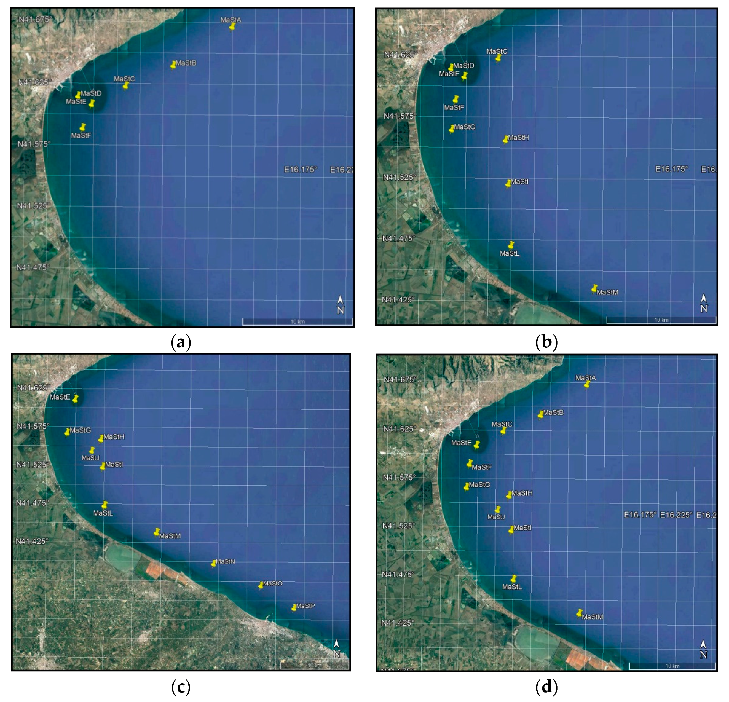
Data of the coastal waters of Manfredonia Gulf, which were acquired in the course of the Coasts and Lake Assessment and Monitoring by PRISMA HYperspectral Mission (CLAM-PHYM) project, [23,24] were exploited to calculate the error in the parametrization of the bio-optical models and to evaluate the capability of remote data to adequately retrieve the concentrations of coastal and inland water constituents using local, daily, and total bio-optical models.

2. Materials and Methods

2.1. Study Area

The study area is a large and shallow gulf located in the western part of the southern Adriatic Sea (Figure 1b), which is named after the town of Manfredonia. This town is an important fishing and sailing city because the Manfredonia Gulf is one of the most representative marinas in Italy in terms of its position and size [25]. The northern border of the gulf is formed by the Gargano Promontory. This hilly promontory is the most prominent coastal bulge of the Adriatic Sea and is entirely situated within Gargano National Park [26]. The southern border is formed by the estuary of the Ofanto River, which represents the main sediment supply in these coastal waters. The sediments of this river are distributed toward the north and northwest by an anticyclonic gyre which is generated by the current of the Nord Adriatic (Figure 1b) [27]. Other continental inputs into the gulf are represented by three seasonal rivers, but their sediment supply is limited (Figure 1b) [28]. The mechanisms that influence the spatial distribution of the surface sediments in the gulf are described by [29]. The authors summarized that the coarser materials are supplied at up to 20 m in depth by the shelf current and the fine-grained sediments are supplied at a higher depth by the Nord Adriatic current which flows offshore in a southerly direction near the Gargano Promontory (Figure 1). Moreover, the sediment transportation due to the Nord Adriatic current is responsible for the significant increase in the bathymetric gradient, starting from the 30 m isobath (Figure 1b, [30]).

In additional to being a key economic and tourism asset for Italy, Manfredonia Gulf is a very productive nursery area of the European sardine (sardine pilchardus). A traditional trawl fishery (“Bianchetto fry” fishery), which was banned in 2010, exploited the high availability of sardines during certain periods of the year [31,32]. The literature clearly underlined the important ecological role of this species, together with anchovies, in the Adriatic and Mediterranean ecosystems [33,34]. However, this important ecosystem is threatened by the agricultural, industrial, and urban activities of this coastal zone [28,35,36,37].

Therefore, the monitoring of these coastal waters plays a crucial role in sustaining this important and vulnerable ecosystem. The monitoring of the coastal waters of the Manfredonia Gulf has mainly been performed by ship and platform surveys [28,38,39,40,41,42,43]. In terms of monitoring with remote data, few works have been carried out to evaluate and minimize the errors in the measurements that were retrieved from remote data [28,44,45].

The results of previous in situ campaigns exhibited that these coastal waters are characterized by a low concentration of the nutrients [28,40,41] and by limited circulation, which is mainly affected by the wind [43]. The status of these coastal waters was classified as oligotrophic by [38,40,42,43], mesotrophic by [41] and eutrophic by [28]. These differences in classification are due to the different metrics used to classify the trophic states, but all methods include measurements of chlorophyll-a concentration as an indicator of phytoplankton biomass [46]. Chlorophyll-a concentrations, which were measured during these mentioned in situ surveys, varied from 0.5 to 10.31 mgm⁻³ [28,38,39,40,41,42,43].

2.2. In Situ Data

The coastal waters of the Manfredonia Gulf were monitored over four days using ship, airborne, and satellite surveys [24]. With reference to in situ surveys, the daily monitoring strategy aimed to cover the total spatial variability of the coastal waters. Measurement locations were identified at a distance of about 4 km from the coastline and between bathymetric lines of 10 and 15 m (Figure 1b) in accordance with the Ocean Optics Protocols for Satellite Ocean Color Sensor Validation [3] and with the literature [28,38,39,40,41,42,43]. Some of these measurement locations were monitored several times as, shown in Figure 2. A total of 36 water columns were characterized under specific conditions of weather (i.e., clear-sky and sea surface wind speed less than 5 m/s) to achieve a comprehensive dataset that allowed us to develop bio-optical models, and to validate these models and their results [3,5,6,9,21,47,48,49]. For these purposes, sky and water surface radiances, bio-physico-chemical parameters, and samples of the water columns were collected at each station.

Sky and water surface radiances (i.e., above-water radiances) were acquired with a hyperspectral spectrometer (i.e., FieldSpec FR PRO spectrometer, Analytical Spectral Devices (ASD), Boulder, CO, USA), which provides continuous coverage of visible, near-infrared, and short-wave infrared spectral domains. In terms of the visible region, the spectral characteristics of the spectrometer meet the spectral requirement for measuring in situ AOPs because its FWHM is equal to 3 nm [21]. Moreover, the spectral sampling interval of the spectrometer is equal to 1.4 nm and the accompanying software resampled the spectra to 1 nm. In accordance with the Ocean Optics Protocols for Satellite Ocean Color Sensor Validation [47] and with the literature [12,14,15,19,48,49], the usual method for measuring remote sensing reflectances above water surface (R_rs) was thoroughly applied for each acquisition: (i) the radiance was acquired with a field of view of 3°. (ii) The radiance was measured from the deck of the ship to a portion of the sea where the multi-parametric platform was dived. (iii) The radiometer was alternately pointed downward to view the sea and upward to view the sky at the required zenith angle θ, equal to 45°, and at the required azimuth angle φ, equal to 90° or 180°, where φ was calculated with respect to the sun’s azimuth angle, where the ship’s heading should point towards the sun (i.e., azimuth angle equal to 0°). In order to verify the view angle, the radiometer was equipped with a goniometer. (iv) After each pair of radiance measurements from the sea and sky, the radiometer acquired the reflectance of a horizontal grey reflectance plaque, which had a known bidirectional reflectance distribution function (BRDF). Each water column was characterized with at least 10 series of measurements.

The bio-physic-chemical parameters of the water column were collected with three different probes to measure chlorophyll-a fluorescence along the water column: ELFO and TFLAP, which are equipped with probe submersible pump-and-probe fluorometers developed at the Laboratory of Biophysics of the University of Moscow [50,51], SeaBird Electronics SBE 911-plus Conductivity-Temperature-Depth (CTD). The literature highlighted that the water sample must be representative of the radiation, which is received by remote sensor and 90% of this radiation comes from the first optical depth of the water column, which corresponds to 0.6 times the Secchi disk depth [52,53]. At each measurement station, water samples were collected at three different depths, which were selected within the first optical depth before mixing together in a single container. The first sampling was done at the surface and the two other depths were identified from time to time based on the value of the Secchi disk depth (i.e., 0.6 and 0.3 times Secchi disk depth). The mean and standard deviation values of every Secchi disk depth that were acquired during the in situ survey were equal to 5 and 1.61 m. Therefore, integrated water samples were taken to calculate the concentration of total suspended particulate matter and the absorption spectra of colored dissolved organic material, depigmented and pigmented particles.

In accordance with Ocean Optics Protocols for Satellite Ocean Color Sensor Validation [54], concentrations of total suspended particulate matter were determined by applying the gravimetric procedures developed by Strickland and Parsons [55].

The absorption of colored dissolved organic material was measured in accordance with Ocean Optics Protocols for Satellite Ocean Color Sensor Validation [6]: (i) integrated water samples were filtered through 0.2 µm Nucleopore membrane filters; (ii) the filters were stored in the dark under refrigeration (4° to 8° C); (iii) the filters were analyzed on board within 24 hours using a Perkin Elmer spectrophotometer 550A model (10 cm cuvette pathlength); (iv) absorbance data were converted to obtain the absorption coefficient [6].

In accordance with Ocean Optics Protocols for Satellite Ocean Color Sensor Validation [6], integrated water samples were used to measure the absorption spectra of the depigmented particles and phytoplankton: (i) the absorption spectra of total particles retained in the GF/F filters were measured using a laboratory spectrophotometer and the filter-pad technique [56]; (ii) the filters were then treated with cold Methanol to extract pigments and the absorption spectra of the depigmented particles of these bleached filters were measured; (iii) the absorption spectrum of phytoplankton was derived by subtracting the absorption spectra of depigmented particles from the absorption spectra of total particles.

2.3. Airborne and Satellite Data

Precursore Iperspettrale della Missione Applicativa (PRISMA) is an Earth observation system used by the Italian Space Agency (ASI) that includes a hyperspectral sensor and a panchromatic camera; the spacecraft was launched on 22 March 2019. The ASI called for proposals in 2009 and five scientific studies started in 2011 to support the exploitation of PRISMA hyperspectral images for environmental applications [23]. The CLAM-PHYM project, which was one of these five projects, aimed to verify the potential of PRISMA hyperspectral sensors for applications in coastal and inland waters [23]. In this framework, an in situ survey was simultaneously (or quasi-simultaneously) performed with multi- and hyperspectral sensors on board airborne and satellite platforms (

Table 1. Acquisition days of all surveys (i.e., in situ, airborne, and satellite).

Day of Acquisition	Surveys
	In Situ	Airborne	Satellite	Satellite	Satellite
2 August 2011				Landsat TM	MODIS
8 August 2011	ship				MODIS
9 August 2011	ship	MIVIS	CHRIS	Landsat TM	MODIS
12 August 2011	ship				MODIS
18 August 2011			CHRIS	Landsat TM	MODIS
24 August 2011	ship				MODIS
25 August 2011				Landsat TM	MODIS

).

Hyperspectral airborne data were acquired by a Multispectral Infrared and Visible Imaging Spectrometer (MIVIS) sensor on board the CASA C212 aircraft [57]. MIVIS data were acquired over the Manfredonia Gulf on 9 August 2011. This acquisition was performed at an absolute altitude of 1,500 m a.s.l. (i.e., the pixel ground resolution was about 3 m). The MIVIS survey included three flights that were oriented NW/SE and parallel to one another.

Hyperspectral satellite data were recorded by a Compact High-Resolution Imaging Spectrometer (CHRIS) sensor on board a PRoject for On-Board Autonomy (PROBA) satellite [58,59]. The satellite acquisitions were obtained through the European Space Agency Category 01 (ESA-CAT-01) project (ID7977). This project aims to cooperate in the assessment of bio-optical models in coastal waters using hyperspectral data. Within this framework, two CHRIS acquisitions over the Manfredonia Gulf were carried out in August 2011.

Multispectral satellite data were recorded by Moderate Resolution Imaging Spectroradiometer (MODIS), and Thematic Mapper (TM) sensors on board Aqua and Landsat5 satellites, respectively. The MODIS sensor acquires data about the coastal area of the Manfredonia Gulf daily. Therefore, four images were taken in tandem with ship surveys (Table 1). Four Landasat5 TM acquisitions were carried out in the coastal area of the Manfredonia Gulf in August 2011 and one of these was acquired alongside a ship survey (Table 1).

2.4. Bio Optical Model

The relationship between the APOs and IOPs used resembles that of previously published bio-optical models for optically deep waters [12,13,14,15,19,20]:

$$R_{rs}=F\ast \frac{b_b}{a+b_b}$$

(1)

where R_rs are remote sensing reflectances, F is a parameter related to the illumination fields and optical properties of the water surface, which was assessed by Hydrolight software [12,14,15,19], and a and b_b are the absorption and backscattering spectra of the water columns, which are given by:

$$\begin{array}{l}a=a_w+{\displaystyle {\sum }_{j=1}^n{a}_j}\ast C_j\\ b_b={b_b}_w+{\displaystyle {\sum }_{j=1}^n{b}_{bj}}\ast C_j\end{array}$$

(2)

where a_w and b_bw are the absorption and backscattering spectra of pure water, a, b_b and C are the absorption, backscattering, and concentrations of the jth water constituent. Therefore, the development of a bio-optical model consists of identifying the absorption and backscattering spectra of each water constituent taken into consideration. This work took into consideration three water constituents: colored dissolved organic material, depigmented particles and pigmented particles. As pigmented particles are usually associated with chlorophyll-a, which represents its main pigment [12,13,14,15,16,18,19,20], Equation (2) is given by:

$$\begin{array}{l}a=a_w+a_{Chla}\ast C_{Chla}+a_{CDOM}\ast a_{CDOM}(440)+a_{TR}\ast C_{TR}\\ b_b={b_b}_w+b_{bChla}\ast C_{Chla}+b_{bCDOM}\ast a_{CDOM}(440)+{b_b}_{TR}\ast C_{TR}\end{array}$$

(3)

where a, and b_b are the absorption and backscattering of chlorophyll-a particles (Chla), colored dissolved organic material (CDOM), and tripton (TR) particles C is the concentration of chlorophyll-a particles (Chla), and tripton (TR) particles and a_CDOM (440) is the absorption of the colored dissolved organic material at 440 nm, which was measured in laboratory.

Some absorption and backscattering spectra that were used as inputs into the bio-optical models were sourced from the literature: the absorption and backscattering spectra of pure water [60,61], the backscattering spectra of colored dissolved organic material, chlorophyll-a, and tripton particles [62].

Other absorption and backscattering spectra were obtained with in situ data. The absorption spectra of colored dissolved organic material (a_CDOM) was described with the exponential slope given by [63]:

$$a_{CDOM}=a_{CDOM}(443)e^{(-0.0176(\lambda -443))}$$

(4)

where a_CDOM (443) is equal to $\frac{a_{CDOM}(412)}{1.17}$ (a_CDOM (412) was measured in a laboratory).

After measuring in a laboratory, the absorption spectra of Chla and TR were normalized with respect to their respective concentrations and resultant spectra were used as inputs into the bio-optical models. As the measurements of Chla concentrations (C_Chla) were not available, C_Chla was given by [14]:

$$C_{Chla}(mg/m^3)=2.7146\ast (fluorescence,mV)-1.8474$$

(5)

where fluorescence data were taken up to the first optical depth with three different probes [50,51]. The range of resultant concentrations was comparable with the range of previous in situ data [38,39,40,41,42,43]. As the height of the phytoplankton absorption peak at 676 nm, corrected for baseline (a_Chla-LH (676)), is significantly related to chlorophyll-a concentration [63,64,65], it was estimated to validate the results of the algorithm [14]. The method for removing the baseline between 650 and 715 nm from the peak at 676 nm, which was proposed by [65], was performed by evaluating the a_Chla-LH (676) of every measured phytoplankton absorption. a_Chla-LH (676) was given by [65]:

$$a_{Chla-LH}(676)=a_{Chla}(676)-\left[\frac{a_{Chla}(715)-a_{Chla}(650)}{715-650}\ast \left(676-650\right)+a_{Chla}(650)\right]$$

(6)

where a_Chla (650), a_Chla (676), and a_Chla (715) are equal to phytoplankton absorption at 650, 676, and 715 nm, respectively, which were measured in a laboratory. Therefore, Equation (5) was used to calculate every Chla concentration because these concentrations were in good agreement with the evaluated values of a_Chla-LH (676) showing the slope of the best correlation line equal to 0.0064 m²/mg, its intercept equal to 0.0035 m⁻¹, and a coefficient of determination (R²) equal to 0.87.

As the concentrations of total suspended particulate matter (C_SPM), which were measured in a laboratory, include organic detritus and tripton, the concentration of tripton (C_TR) was separated by (C_SPM) using [12]:

$$C_{TR}(g/m^3)=C_{SPM}(g/m^3)-0.07C_{Chla}(mg/m^3)$$

(7)

Equation (1) has to be inverted to retrieve the concentrations of the water constituents and several mathematic procedures for inverting it were reported in the literature [11]. The procedure described by [15,19] was performed using the ad hoc software developed in Interactive Data Language (IDL). The outputs of the IDL procedure consist of water constituent concentrations and the difference between modeled and measured R_rs spectra, which were quantified with the percentage of the root mean square (RMS): $RMS\%=100\ast \sqrt{\frac{{(R_{rs\_modelled}-R_{rs\_measured})}^2}{{(R_{rs\_measured})}^2}}$.

R_rs spectra measured with ASD instruments were corrected by a variable amount of reflected sky radiance before using to them to validate the model [66].

To compare the results of model validation, the differences between all modeled and measured R_rs spectra were summarized with mean $\left(mea{n}_{RMS\%}=\frac{1}{N}\ast {\displaystyle \sum _{i=1}^{N}RMS{\%}_i}\right)$ and standard deviation $\left({\sigma }_{RMS\%}=\sqrt{\frac{{\displaystyle \sum _{i=1}^N{(RMS{\%}_i-mea{n}_{RMS\%})}^2}}{N}}\right)$ values of the RMS%.

To validate the results of the models, the retrieved concentrations of the water constituents were compared with the ones measured in situ. All their differences were quantified with the mean $\left(mea{n}_{bias}=\frac{1}{N}\ast {\displaystyle \sum _{i=1}^N(C_{measured}-C_{modelled})}\right)$ and standard deviation $\left({\sigma }_{bias}=\sqrt{\frac{{\displaystyle \sum _{i=1}^N{(bia{s}_i-mea{n}_{bias})}^2}}{N}}\right)$ of bias values, relative bias $\left(bias\%=\frac{\sqrt[]{{(C_{measured}-C_{modelled})}^2}}{(C_{\max }-C_{\min })})\ast 100\right)$ and Kling–Gupta efficiency $\left(KGE=1-\sqrt{{(R-1)}^2+{(\frac{{\sigma }_{modelled}}{{\sigma }_{measured}}-1)}^2+{(\frac{{\mu }_{modelled}}{{\mu }_{measured}}-1)}^2}\right)$ where R is the linear correlation between modeled and measured concentrations, σ and μ are standard deviation and mean values of modeled and measured data [67]. The Kling–Gupta efficiency (KGE) value, which is often used to calibrate and evaluate hydrological models, was chosen because it expresses, in a single number, the similarity between modeled and measured data using three constitutive components: correlation, mean and standard deviation of bias. A KGE value equal to one indicates perfect agreement between modeled and measured data; most of the papers considered positive values of KGE as indicative of “good” model simulations, whereas negative values of KGE are considered “bad” e.g., [68].

Every result was also evaluated by the slope, intercept, and coefficient of determination (R²) of the best regression line between the retrieved and measured data.

2.5. Local, Daily, and Total Bio Optical Models

One of the major error sources is the parameterization of the bio-optical model (i.e., the selection of the absorption and backscattering spectra of water constituents that were taken into consideration [9,10,11]). The literature highlighted that “simultaneous and co-located” data are a fundamental requirement for minimizing these errors. In other words, remote data used to retrieve water constituent concentrations have to be “simultaneous and co-located” with respect to the absorption and backscattering spectra that are used to develop the models, with respect to the R_rs spectra that are used to validate the models, and with respect to the water constituent concentrations that are used to validate their results [5,6,7,9,10,11,21]. To evaluate these errors, different absorption and backscattering spectra were identified in accordance with the position and time of the in situ survey, whereas the same measurements were used to validate these models and their results. Therefore, the water constituents of each water column were retrieved using three bio-optical models: local, daily, and total models.

The local bio-optical model was the best model for resolving the spectral characteristic of each water column. To better resolve the optical properties of each water column, a local bio-optical model was developed for each measurement station using the absorption spectra of the water column that was characterized on that particular day. Therefore, the absorption spectra of Chla, CDOM, and TR used for one local model were different from the spectra used for other models. However, the same backscattering spectra of pure water [60,61], chlorophyll-a particles, colored dissolved organic material, and tripton particles [62] and the same absorption of pure water [60,61] were used as inputs not only into every local bio-optical model, but also into every daily and total bio-optical model. The number of local bio-optical models developed was thirty-six, equal to the number of water columns that were monitored.

The daily bio-optical model was the model that adequately characterized the daily spatial variations in the optical properties that were monitored on that day. All combinations of daily a_Chla, a_CDOM, and a_TR were analyzed to identify the daily average spectra that minimize the difference between modeled and in situ measurements of R_rs and water constituent concentrations. Therefore, these average daily spectra were used as inputs into the daily bio-optical model of that day. The number of daily bio-optical models developed was four, equal to the number of measurement days.

The total bio-optical model was the model which adequately characterized temporal and spatial variations in the optical properties that were monitored during the in situ survey. The same careful analysis that was performed for daily bio-optical models was achieved to identify the total average spectra of a_Chla, a_CDOM, and a_TR, which minimize the difference between the modeled and measured data.

In situ measurements of AOPs (i.e., R_rs spectra corrected by a variable amount of reflected sky radiance [66]) and IOPs (i.e., a_Chla, a_CDOM, and a_TR spectra) used to develop and validate these bio-optical models were characterized with spectral ranges from 400 to 750 nm and with FWHM bandwidths equal to 1 nm.

Table 2. Values of mean and standard deviation (σ) of in situ data of each day and all days in total.

8 August 2011	CChla (mgm−3)	aCDOM 440 (m−1)	CTR (gm−3)
Mean	0.872	0.061	2.345
σ	0.354	0.077	0.803
9 August 2011	CChla (mgm−3)	aCDOM 440 (m−1)	CTR (gm−3)
Mean	0.467	0.011	3.141
σ	0.341	0.023	0.718
12 August 2011	CChla (mgm−3)	aCDOM 440 (m−1)	CTR (gm−3)
Mean	0.799	0.097	5.372
σ	0.560	0.136	2.241
24 August 2011	CChla (mgm−3)	aCDOM 440 (m−1)	CTR (gm−3)
Mean	0.686	0.143	7.433
σ	0.273	0.115	0.890
All Days	CChla (mgm−3)	aCDOM 440 (m−1)	CTR (gm−3)
Mean	0.694	0.084	4.939
σ	0.410	0.110	2.392

shows the in situ data (i.e., concentrations of Chla, absorption of CDOM at 440 nm, and concentrations of TR) that were used to validate the results of the local, daily, ad total bio-optical models.

2.6. Retrieval Water Constituents from Remote Data Using Local, Daily, and Total Bio Optical Models

Multi- and hyperspectral data were acquired during these surveys (see Table 1). Developed and validated local, daily, and total bio-optical models were used to evaluate their spectral capabilities to characterize these coastal waters. To highlight only the errors in their spectral capabilities, these remote data were simulated using R_rs measured in situ. As mentioned above, the in situ measurements of AOPs and IOPs used to develop and validate the models were characterized with a spectral range from 400 to 750 nm and with a FWHM bandwidth of 1 nm. Therefore, these spectra were resampled in accordance with the spectral characteristics of these remote data.

The satellite configuration of CHRIS data utilized during this campaign was mode 2. This configuration is also called “water bands”. To identify the best CHRIS configuration for characterizing these coastal waters, two imaging configurations were evaluated, mode 1 and mode 2. The CHRIS sensor, in configuration mode 1, records 62 contiguous spectral bands from 406 to 1003 nm at a spectral resolution of about 10 nm. The CHRIS sensor, in configuration mode 2, records 18 non-consecutive spectral bands from 410 to 1038 nm at a spectral resolution of about 15 nm. Actually, the wavelength allocations of CHRIS data acquired in mode 1 are the nominal values in accordance with the CHRIS data format [59], whereas the spectral characteristics of CHRIS data acquired in mode 2 are the actual wavelengths for the operating temperature, detailed within their Hierarchical Data Format (HDF)files, obtained during the summer of 2011.

The spectral characteristics of MIVIS data were certified by the spectral calibration performed in May 2011 by the ArgonST Imaging Group. The first spectrometer measures had twenty contiguous spectral bands from 431 to 838 nm at an average spectral resolution of 20 nm.

The multispectral data acquired during the surveys were MODIS and TM data.

CHRIS data acquired using mode 1 configuration and PRISMA data were added to this dataset to evaluate their spectral capabilities in characterizing these coastal waters. Therefore, R_rs measured in situ were also resampled in accordance with the spectral characteristics of PRISMA data: a hyperspectral camera records data in 60 contiguous spectral bands covering the spectral range from 400 to 1000 nm, with an average spectral resolution of 10 nm. [23,69].

Equations (1) and (2) used by local, daily, and total bio-optical models correspond to a system of m equations (where m is equal to the number of bands) with n unknowns (where n is equal to number of water constituents taken into consideration). In the spectral range from 400 to 750 nm, the number of bands of ASD, CHRIS mode 1 and mode 2, MIVIS, MODIS and PRISMA data (i.e., 351, 37, 14, 16, 8, and 35, respectively) is greater than the number of water constituents taken into consideration (i.e., chlorophyll-a particles, colored dissolved organic material, and tripton particles). However, the number of bands in the Landsat TM data in this spectral range is equal to three. Therefore, the same water constituents were retrieved one at a time using, as an input, the known concentrations of the other two water constituents, and the value of RMS% was equal to the average of the three RMS% obtained.

3. Results

3.1. Validation of Local, Daily, and Total Bio-Optical Models

After correcting by a variable amount of reflected sky radiance [66], R_rs spectra which were measured with ASD instruments were used to validate local, daily, and total bio-optical models.

Table 3. The results of validation procedure of local, daily, and total bio-optical models.

08 August 2011	Local	Daily	Total
meanRMS%	0.2%	1.4%	6.5%
σRMS%	0.1%	0.6%	1.2%
09 August 2011	Local	Daily	Total
meanRMS%	0.2%	3.1%	3.7%
σRMS%	0.1%	0.8%	1.6%
12 August 2011	Local	Daily	Total
meanRMS%	0.1%	3.1%	5.7%
σRMS%	0.0%	1.4%	2.7%
24 August 2011	Local	Daily	Total
meanRMS%	0.1%	3.1%	5.8%
σRMS%	0.1%	2.2%	3.2%
All Days	Local	Daily	Total
meanRMS%	0.1%	3.8%	5.3%
σRMS%	0.1%	1.7%	2.0%

summarizes the results of the model validation (i.e., the difference between modeled and measured R_rs), which were quantified with the mean (mean_RMS%) and standard deviation (σ_RMS%) of RMS% values.

The validation of local bio-optical models highlighted very good convergence between modeled and measured R_rs spectra (i.e., the mean and standard deviation values of RMS% are close to 0%) and the validation of daily and total models showed good convergence between the modeled and measured R_rs spectra. In other words, the mean and standard deviation values of RMS% obtained by validating the total model are smaller than 5.3%–2.0% and these values are slightly greater than the ones that were calculated by validating the daily models, whereas, these values are quite greater than the ones that were calculated by validating the local models.

With reference to each measurement day, the mean and standard deviation values of RMS% varied from day to day, but the values obtained by validating the local models were always smaller than the ones that were obtained by validating the daily models and these values are always smaller than the ones that were obtained by validating the total model.

3.2. Validation of Local, Daily, and Total Bio-Optical Model Results

The concentrations of the water constituents that were retrieved using local, daily, and total bio-optical models were compared with the ones that were measured in situ, which are summarized in the Table 2. As mentioned above, the differences between these water constituent concentrations were quantified with the mean (mean_bias) and standard deviation (σ_bias) of the bias values, relative bias (bias%), and Kling–Gupta efficiency (KGE).

The mean and standard deviation values of bias, and values of bias% and KGE varied from day to day, but all these results highlighted that the chosen models adequately retrieved the concentrations of water constituents in Manfredonia Gulf because every value of bias% is smaller than 40% and every value of KGE is positive. Only one value of bias% is close to 40%: the error in C_Chla was calculated by the total bio-optical model using the 24 August dataset (i.e., 42%). Only two values of KGE are close to 0.2: the error in a_CDOM at 440 nm was calculated by the total bio-optical model using the 9 August dataset (i.e., 0.19) and the error in C_Chla was calculated by the total bio-optical model using the 24 August dataset (i.e., 0.14). Moreover, C_TR retrieved using every model highlighted very good agreement between the modeled and measured data: the mean values of bias% evaluated by local, daily, and total models are smaller than 10% (i.e., 3%, 5%, and 6%, respectively) and the mean values of KGE evaluated by local, daily, and total models are close to one (i.e., 0.96, 0.92, and 0.91, respectively). Moreover, most water constituents calculated by local models highlighted KGE values close to one except four of the values: errors in a_CDOM at 440 nm calculated using the 8, 9, and 22 August datasets (i.e., KGE values close to 0.5) and the error in C_Chla calculated using the 24 August dataset (i.e., KGE values close to 0.5).

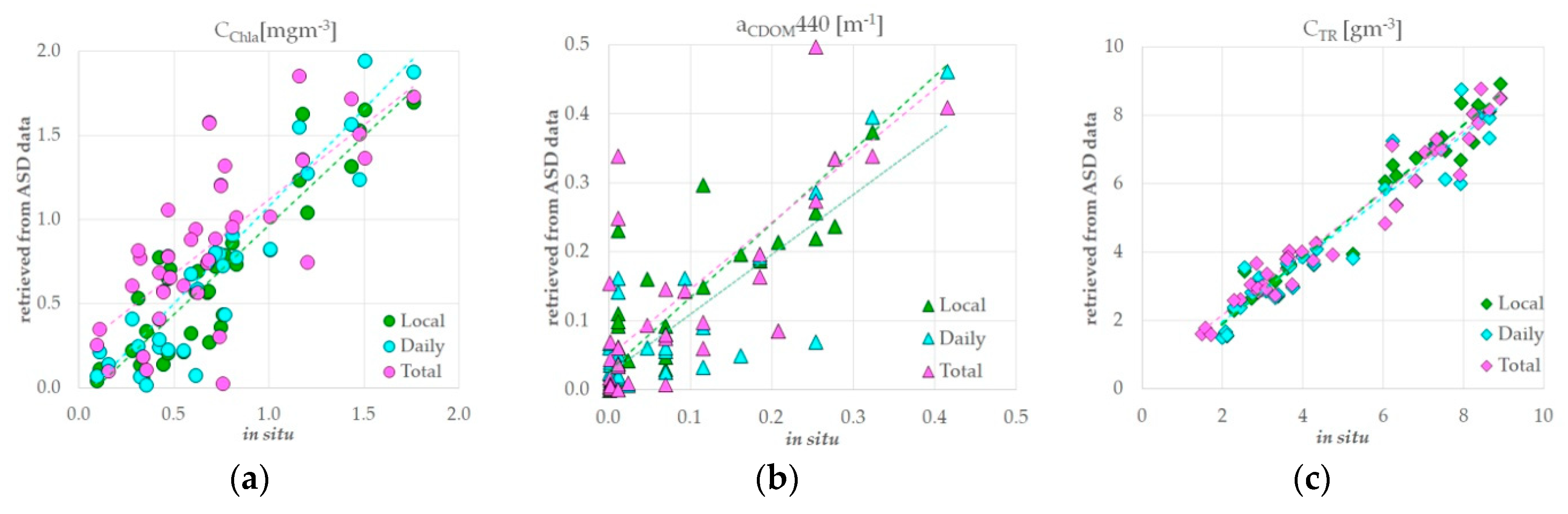
The relationships between the C_Chla, a_CDOM at 440 nm, and C_TR of all water columns that were retrieved with local, daily, and total bio-optical models and in situ measurements are shown in three scatter plots (Figure 3).

Because all the best correlation lines are close to the 1:1 line, every chosen model adequately resolves the variability in water constituent concentrations in Manfredonia Gulf.

Table 4. The errors in C_Chla, a_CDOM at 440 nm, and C_TR evaluated using local, daily, and total bio-optical models.

Bio−Optical Models		Slope	Intercept	R2	meanbias	σbias	bias %	KGE
CChla (mgm−3)	Local	1.06	−0.09	0.83	0.05	0.20	10%	0.80
	Daily	1.16	−0.08	0.77	−0.03	0.27	12%	0.65
	Total	0.88	0.23	0.56	−0.15	0.32	17%	0.62
aCDOM 440 (m−1)	Local	1.07	0.03	0.77	−0.03	0.07	11%	0.54
	Daily	0.87	0.02	0.70	−0.01	0.06	11%	0.78
	Total	0.97	0.05	0.54	−0.05	0.10	15%	0.31
CTR (gm−3)	Local	0.97	0.03	0.97	0.12	0.35	3%	0.96
	Daily	0.87	0.23	0.92	0.23	0.52	5%	0.92
	Total	0.85	0.51	0.94	0.14	0.54	6%	0.91

summarizes the errors in C_Chla, a_CDOM at 440 nm, and C_TR, which were calculated to validate the results of the local, daily, and total models.

These results highlight that the error increases from the local to the daily bio-optical models and from the daily to the total bio-optical models. With reference to C_Chla and a_CDOM at 440 nm, the application of the total model with respect to the local model increases bias% values by about 50%. With reference to C_TR, the application of the total model with respect to the local model increases bias% values by 100%. The KGE values calculated for C_Chla, a_CDOM at 440 nm and C_TR increase by 18%, 23%, and 5%. However, C_Chla, a_CDOM at 440 nm, and C_TR obtained by the total model are in very good agreement with the in situ data: R² values calculated are greater than 0.50; bias% values are lower than 17%; KGE are greater than 0.31.

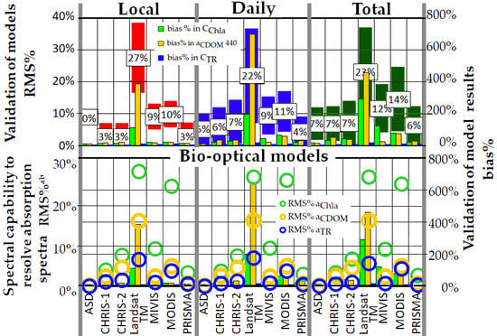
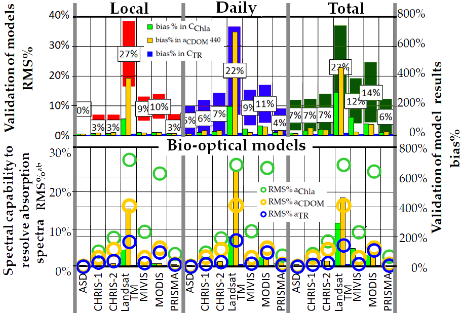
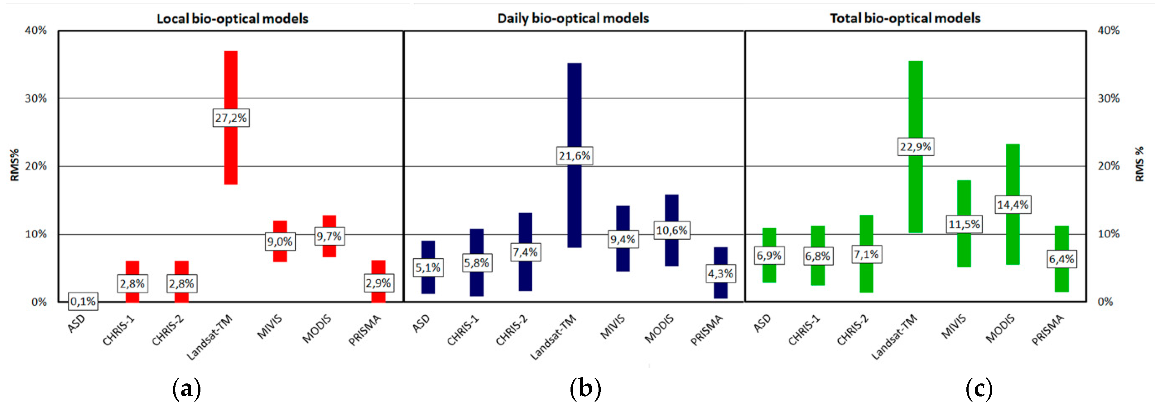
3.3. Local, Daily, and Total Bio-Optical Models Applied to Remote Data

Before applying the remote data, the developed models and R_rs acquired with the ASD instruments were spectrally resampled with respect to the spectral characteristics of CHRIS mode 1 and mode 2, Landsat TM, MIVIS, MODIS, and PRISMA data. The validations of local, daily, and total bio-optical models, which were applied to simulated data, were performed by calculating the differences between the modeled and measured R_rs spectra. These differences were quantified with mean values of RMS% ± their standard deviations (Figure 4).

The validation of the models applied to the remote data highlighted that the smallest values of RMS% were calculated from PRISMA simulated data and the greatest values were calculated from Landsat TM simulated data. RMS% values obtained from CHRIS mode 1 are comparable with the values obtained from the CHRIS mode 2 simulated data and these values are slightly greater than the ones that were calculated from the PRISMA simulated data. RMS% values obtained from MIVIS simulated data are greater than the ones obtained from CHRIS mode 1 and mode 2 simulated data and slightly smaller than the ones calculated from MODIS simulated data. The local, daily, and total bio-optical models highlighted the sensors are arranged in the same order according to the RMS% values.

Moreover, every mean and standard deviation value of RMS% increases when applying the daily models compared to the local models and applying the total model compared to the daily models, except for one dataset: the mean value of RMS% calculated from Landsat TM data using local models is greater than the values calculated using daily and total models (i.e., RMS% values are equal to 27.2%, 21.6%, and 22.9%, respectively).

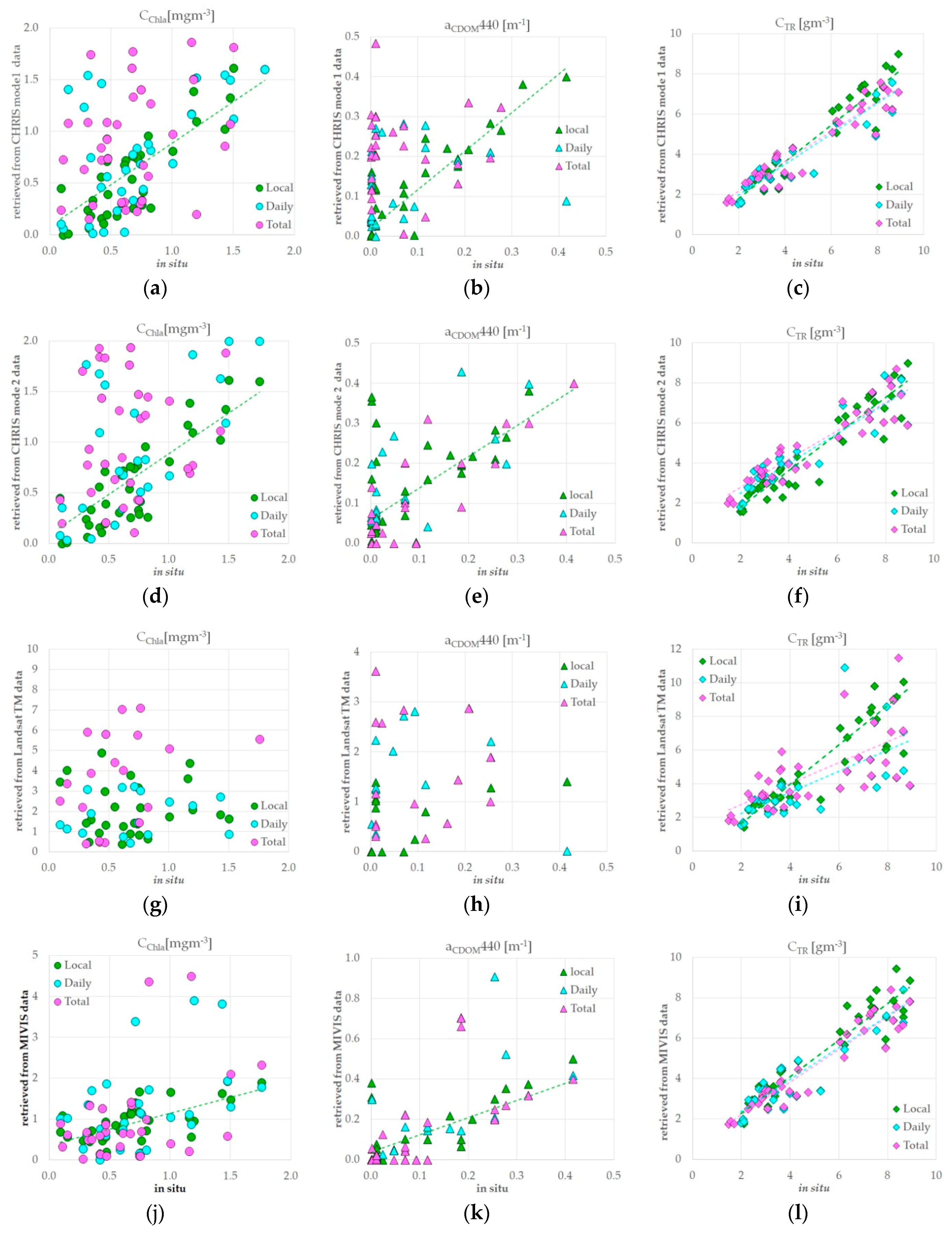
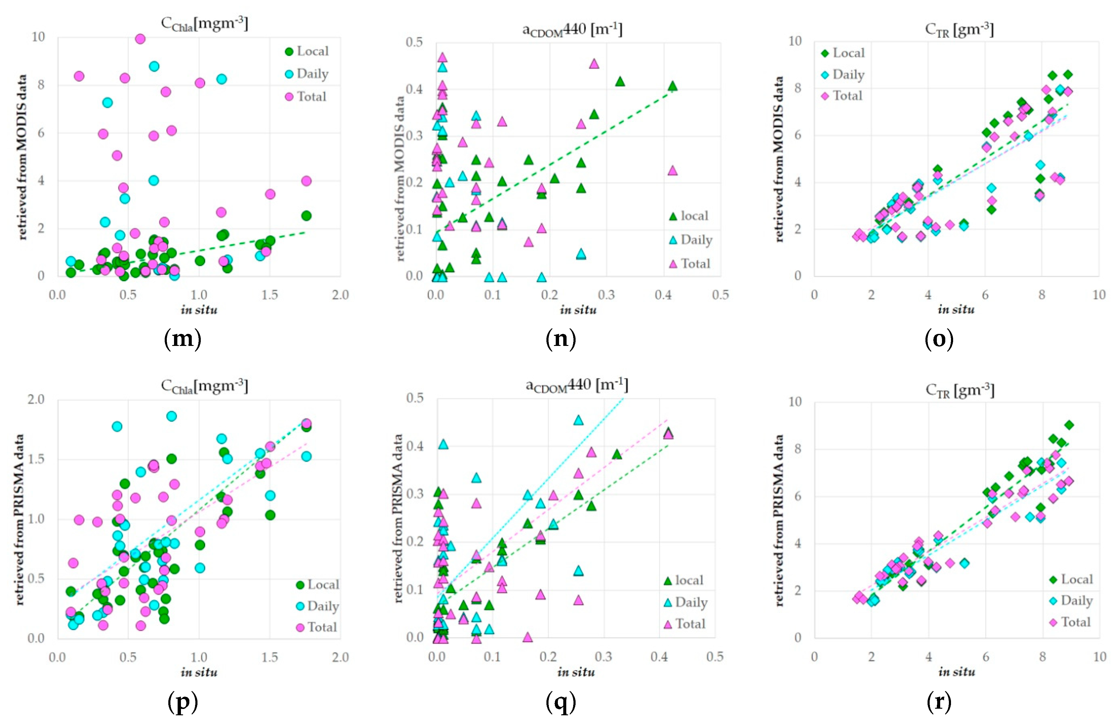
C_Chla, a_CDOM at 440 nm, and C_TR retrieved from CHRIS mode 1, CHRIS mode 2, Landsat TM, MIVIS, MODIS, and PRISMA simulated data using local, daily, and total models were compared with the data measured in situ. Figure 5 shows the scatter plots, which depict every retrieved C_Chla, a_CDOM at 440 nm, and C_TR vs. in situ data.

As some of these results showed great errors, the previous papers offered a useful threshold of error, which helped us to choose only the models that adequately retrieved the water constituents [14,15,19]. This threshold was quantified with the slope of the best regression line between the modeled and measured data, and values of R², and bias%: the slope was smaller than 1.4 and greater than 0.6 [14,15,19], the R² value was greater than 0.30 [15,19], and the bias% values were smaller than 40% [15,19]. With reference to these thresholds, some retrieved concentrations of the water constituents were not taken into consideration.

With reference to C_Chla and a_CDOM at 440 nm, the best regression lines obtained from CHRIS mode 1 and mode 2, MIVIS and MODIS simulated data using daily and total models did not meet these requirements and these results were not taken into consideration (Figure 5a,b,d,e,j,k,m,n). For the same reason, the best regression lines obtained from Landsat TM simulated data using all models to retrieve C_Chla and a_CDOM at 440 nm did not meet these requirements and these results were not taken into consideration (Figure 5g,h). On the other hand, C_TR retrieved from all data using all models met these requirements and these results were taken into consideration (Figure 5c,f,i,l,o,r). Moreover, the results retrieved from PRISMA simulated data using every model were taken into consideration because they also met these requirements (Figure 5p–r).

All errors in C_Chla, a_CDOM at 440 nm, and C_TR calculated from CHRIS mode 1, CHRIS mode 2, Landsat TM, MIVIS, MODIS, and PRISMA simulated data, using all bio-optical models, are summarized in

Table 5. The errors in C_Chla, a_CDOM at 440 nm, and C_TR obtained from CHRIS mode 1 simulated data.

Bio-Optical Models		Slope	Intercept	R2	bias	dev	bias %	KGE
CChla (mgm−3)	Local	0.80	0.08	0.48	0.05	0.43	15%	0.51
	Daily	---	---	---1	−0.13	0.48	21%	0.29
	Total	---	---	---1	−0.26	0.58	31%	0.14
aCDOM 440 (m−1)	Local	0.96	0.02	0.43	−0.02	0.12	19%	0.40
	Daily	---	---	---1	−0.06	0.20	34%	−0.37
	Total	---	---	---1	−0.10	0.28	52%	−1.21
CTR (gm−3)	Local	0.91	0.01	0.89	0.39	0.77	6%	0.89
	Daily	0.76	0.46	0.89	0.67	0.82	10%	0.75
	Total	0.72	0.68	0.90	0.59	0.85	10%	0.75

¹ The best regression line was not taken into account because its R² value was smaller than 0.40.

,

Table 6. The errors in C_Chla, a_CDOM at 440 nm, and C_TR obtained from CHRIS mode 2 simulated data.

Bio-Optical Models		Slope	Intercept	R2	bias	dev	bias %	KGE
CChla (mgm−3)	Local	0.80	0.08	0.43	0.05	0.43	15%	0.51
	Daily	---	---	---1	−0.23	0.56	28%	0.18
	Total	---	---	---1	−0.35	0.74	40%	−0.19
aCDOM 440 (m−1)	Local	0.78	0.06	0.41	−0.04	0.12	19%	0.44
	Daily	---	---	---1	−0.04	0.18	33%	−0.15
	Total	---	---	---1	−0.02	0.37	37%	−1.57
CTR (gm−3)	Local	0.91	0.01	0.89	0.39	0.77	6%	0.89
	Daily	0.74	1.01	0.86	0.20	0.88	9%	0.78
	Total	0.71	1.37	0.85	0.07	0.99	10%	0.75

¹ The best regression line was not taken into account because its R² value was smaller than 0.40.

,

Table 7. The errors in C_Chla, a_CDOM at 440 nm, and C_TR obtained from Landsat TM simulated data.

Bio-Optical Models		Slope	Intercept	R2	bias	dev	bias %	KGE
CChla (mgm−3)	Local	---	---	---1	−0.19	2.45	112%	−3.89
	Daily	---	---	---1	1.87	3.93	197%	−8.03
	Total	---	---	---1	−0.80	6.00	292%	−12.95
aCDOM 440 (m−1)	Local	---	---	---1	0.36	2.66	386%	−22.71
	Daily	---	---	---1	−1.32	4.28	698%	−40.06
	Total	---	---	---1	0.41	2.35	456%	−20.21
CTR (gm−3)	Local	1.16	-0.82	0.60	−0.22	1.49	13%	0.68
	Daily	0.61	1.01	0.45	0.83	1.76	18%	0.65
	Total	0.62	1.53	0.46	0.34	1.84	20%	0.66

¹ The best regression line was not taken into account because it was not close to the 1:1 line and its R² value was smaller than 0.40.

,

Table 8. The errors in C_Chla, a_CDOM at 440 nm, and C_TR obtained from MIVIS simulated data.

Bio-Optical Models		Slope	Intercept	R2	bias	dev	bias %	KGE
CChla (mgm−3)	Local	0.78	0.36	0.43	−0.21	0.38	22%	0.51
	Daily	---	---	---1	−0.42	0.96	45%	0.20
	Total	---	---	---1	1.25	3.91	124%	−3.63
aCDOM 440 (m−1)	Local	1.06	0.05	0.42	−0.05	0.13	20%	0.46
	Daily	---	---	---1	−0.03	0.19	21%	−0.23
	Total	---	---	---1	−0.03	0.22	23%	−0.46
CTR (gm−3)	Local	0.91	0.47	0.88	−0.06	0.83	9%	0.92
	Daily	0.81	0.59	0.91	0.19	0.85	9%	0.82
	Total	0.79	0.78	0.88	0.35	0.76	8%	0.83

¹ The best regression line was not taken into account because it was not close to the 1:1 line.

,

Table 9. The errors in C_Chla, a_CDOM at 440 nm, and C_TR obtained from MODIS simulated data.

Bio-Optical Models		Slope	Intercept	R2	bias	dev	bias %	KGE
CChla (mgm−3)	Local	1.00	0.09	0.46	−0.09	0.44	22%	0.42
	Daily	---	---	---1	0.35	3.19	65%	−1.90
	Total	---	---	---1	−2.10	3.34	78%	−3.41
aCDOM 440 (m−1)	Local	0.73	0.09	0.35	−0.07	0.11	21%	0.03
	Daily	---	---	---1	−0.07	0.35	58%	−0.69
	Total	---	---	---1	−0.29	0.28	74%	−1.41
CTR (gm−3)	Local	0.79	0.29	0.67	0.69	1.43	12%	0.76
	Daily	0.72	0.49	0.70	0.86	1.33	13%	0.70
	Total	0.69	0.68	0.67	0.87	1.38	14%	0.70

¹ The best regression line was not taken into account because it was not close to the 1:1 line and its R² value was smaller than 0.40.

and

Table 10. The errors in C_Chla, a_CDOM at 440 nm, and C_TR obtained from PRISMA simulated data.

Bio-Optical Models		Slope	Intercept	R2	bias	dev	bias %	KGE
CChla (mgm−3)	Local	1.00	0.08	0.52	−0.08	0.39	15%	0.51
	Daily	0.89	0.27	0.44	−0.20	0.41	19%	0.48
	Total	0.76	0.31	0.38	−0.14	0.47	22%	0.51
aCDOM 440 (m−1)	Local	0.81	0.07	0.59	−0.05	0.08	15%	0.35
	Daily	1.25	0.08	0.45	−0.10	0.15	30%	−0.27
	Total	0.88	0.09	0.35	−0.10	0.18	34%	−0.51
CTR (gm−3)	Local	0.93	0.02	0.91	0.30	0.69	6%	0.91
	Daily	0.74	0.59	0.89	0.66	0.85	10%	0.73
	Total	0.72	0.81	0.89	0.57	0.89	11%	0.73

, respectively.

These data highlight that the errors in C_Chla, a_CDOM at 440 nm, and C_TR evaluated from all simulated data decrease by applying the local models compared to the daily models and by applying daily models compared to the total model. This increase in error is appreciably greater than that was observed in the model validations (Table 4), which were carried out on ASD data, except the errors in C_TR. The errors in C_TR obtained from CHRIS mode 1, CHRIS mode 2, MIVIS, MODIS, and PRISMA simulated data are comparable and these values are slightly greater than the errors calculated by the ASD data during the validation of the model results. However, the errors in C_TR obtained from Landsat TM simulated data are appreciably greater than those observed in the model result validation using the ASD data.

With reference to the capability of the models in characterizing these coastal waters, PRISMA simulated data retrieved the water constituents more adequately than other remote data; the errors calculated using the total model highlighted the slopes of the best regression lines greater than 0.72, R² values greater than 0.38, and bias% values smaller than 34%. Only the KGE values evaluated by retrieving a_CDOM at 440 nm with the daily and total models are negative (i.e., −0.54, and −0.67 m⁻¹, respectively). On the other hand, most KGE values obtained by retrieving a_CDOM at 440 nm are negative and most bias% values were greater than 40%.

The greatest error values were found in the Landsat TM simulated data (Table 7) which only adequately retrieved C_TR using every model. With reference to C_Chla and a_CDOM at 440 nm, the best regression lines are not close to the 1:1 line, R² values are smaller than 0.40, bias% values are greater than 100%, and KGE values are negative. With reference to C_TR, the slopes of the best regression lines are greater than 0.62, R² values are greater than 0.46, bias% values are greater than 20%, and KGE values are greater than 0.65.

The errors in C_Chla, a_CDOM at 440 nm, and C_TR obtained from the CHRIS mode 1 simulated data (Table 5) are greater than the ones that were obtained from the PRISMA simulated data (Table 10). It is interesting to note that the errors evaluated from the CHRIS mode 1 and mode 2 data (Table 5 and Table 6) are comparable; the errors of the first dataset are only slightly smaller than those of the second one. The errors evaluated from the MIVIS simulated data (Table 8) are greater than the ones that were obtained from the CHRIS mode 2 simulated data (Table 6) and they are smaller than the ones of the MODIS simulated data (Table 9).

3.4. Spectral Capabilities of Remote Data to Characterize Coastal Water of Manfredonia Gulf

The capabilities of CHRIS mode 1, CHRIS mode 2, Landsat TM, MIVIS, MODIS, and PRISMA data to characterize the coastal water of the Manfredonia Gulf were evaluated by analyzing their spectral capabilities to resolve the absorption spectra of Chla, CDOM, and TR. For this purpose, the absorption spectra measured in laboratory, called the starting absorption spectra, were compared with those using as inputs into the local, daily, and total models, which were resampled in accordance with the spectral characteristics of these remote data. Their differences were quantified using RMS% values, called RMS%^ab.

Table 11. RMS%^ab values between starting a_Chla, a_CDOM, and a_TR spectra and the resampled ones which were used as inputs into local, daily, and total models.

Remote Data	RMS%ab aChla	RMS%ab aCDOM	RMS%ab aTR	between Starting aChla, aCDOM, and aTR Spectra and
CHRIS mode 1	3.76%	2.20%	0.93%	resampled local models
CHRIS mode 2	7.33%	4.27%	1.33%	resampled local models
Landsat TM	27.04% 1	15.37% 1	6.24%	resampled local models
MIVIS	8.82%	2.21%	0.84%	resampled local models
MODIS	23.58%	4.70%	3.52%	resampled local models
PRISMA	3.11%	0.57%	0.51%	resampled local models
CHRIS mode 1	23.74% 1	8.15% 1	3.51%	resampled daily models
CHRIS mode 2	24.13% 1	7.83% 1	3.45%	resampled daily models
Landsat TM	38.02% 1	28.32% 1	7.53%	resampled daily models
MIVIS	25.33% 1	6.20% 1	3.62%	resampled daily models
MODIS	30.99% 1	10.41% 1	4.07%	resampled daily models
PRISMA	19.11%	6.65%	3.48%	resampled daily models
CHRIS mode 1	37.54% 1	9.75% 1	4.24%	resampled total model
CHRIS mode 2	38.42% 1	9.45% 1	4.12%	resampled total model
Landsat TM	54.89% 1	18.09% 1	9.73%	resampled total model
MIVIS	39.02% 1	16.28% 1	5.05%	resampled total model
MODIS	49.47% 1	19.76% 1	6.46%	resampled total model
PRISMA	21.07%	7.67%	3.66%	resampled total model

¹ With reference to the selected threshold, the errors in C_Chla, a_CDOM at 440 nm, and C_TR highlighted that the data do not adequately resolve the variability in this water constituent.

summarizes the resultant RMS% ^ab values.

As the absorption spectra of daily and total models are the averages of the starting absorption spectra, and the spectra averaged to make the total model are greater than those averaged to make the daily models, the RMS%^ab values obtained by comparing the resampled local models are smaller than the RMS%^ab values which obtained by comparing the resampled daily models, with the latter values being smaller than the RMS%^ab values that were calculated by comparing the resampled total model. Moreover, the errors in C_Chla, a_CDOM at 440 nm, and C_TR evaluated from all remote data using the local models are smaller than those obtained using the daily models and these values are smaller than those obtained using the total model.

All remote data highlighted that the RMS% ^ab values evaluated to resolve a_TR are smaller than the ones calculated to resolve a_CDOM, and that these values are smaller than the ones evaluated to resolve a_Chla. Furthermore, the evaluated errors in C_TR are smaller than the ones in a_CDOM at 440 nm, whereas these values are greater than the ones in C_Chla.

The greatest values of RMS% ^ab were evaluated from Landsat TM simulated data and the smallest values of RMS% ^ab were evaluated from PRISMA simulated data. Additionally, errors in C_Chla, a_CDOM at 440 nm, and C_TR evaluated from Landsat TM data are the greatest and the ones that were obtained from PRISMA data are the smallest.

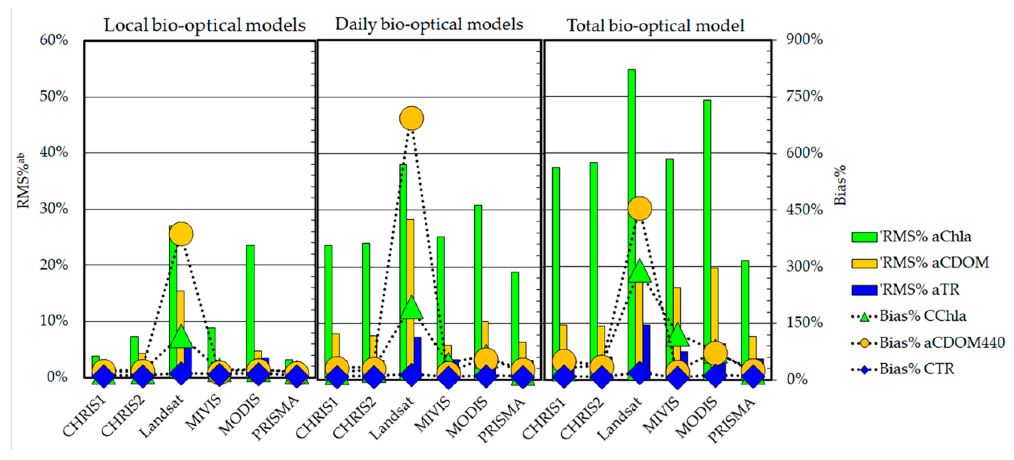
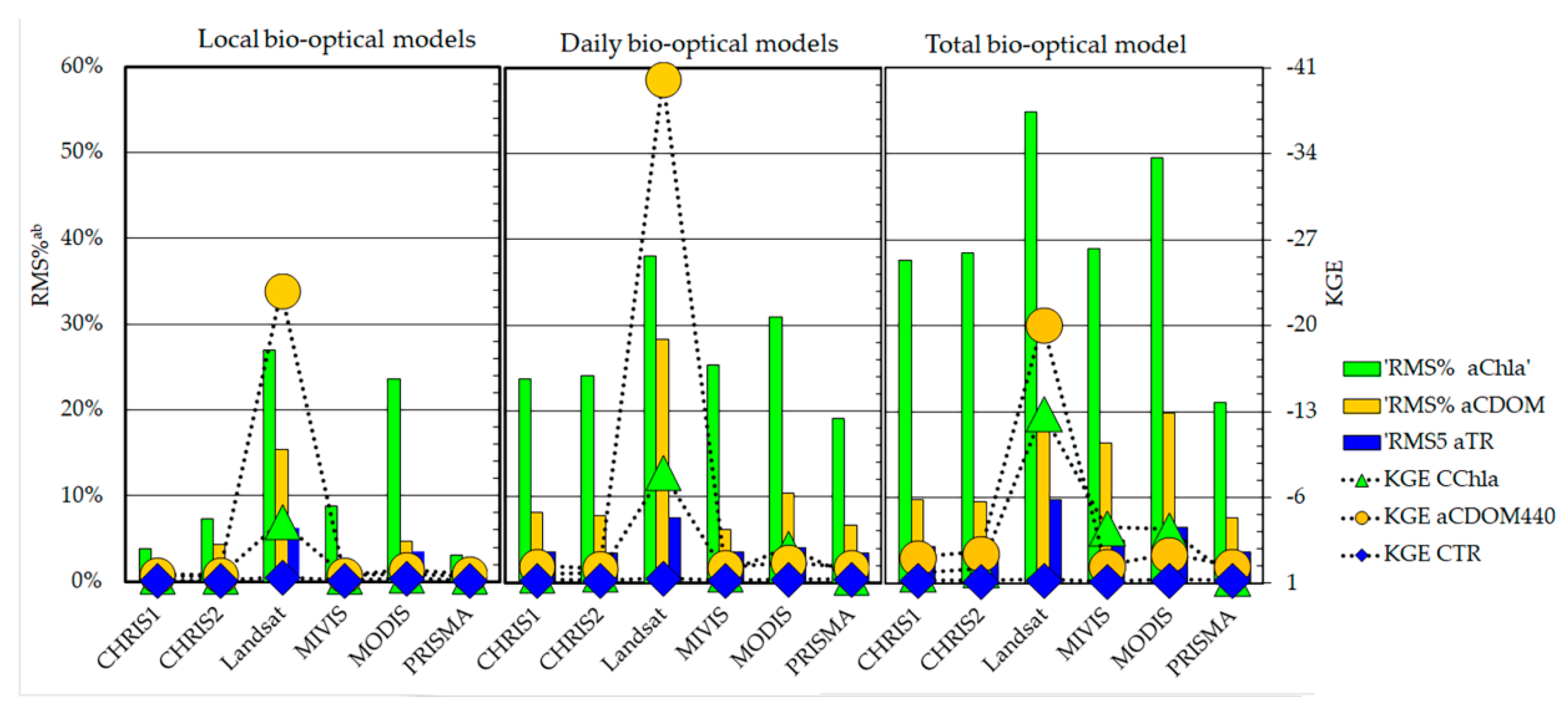
Therefore, the RMS% ^ab values were compared with the mean values of bias% and KGE, which were calculated from these remote data using the local, daily, and total bio-optical models (Figure 6 and Figure 7).

These results highlight that the mean values of bias% and KGE calculated from all data and RMS% ^ab values obtained from all data are correlated (i.e., the linear correlations between mean values of bias% and RMS% ^ab evaluated with a_Chla, a_CDOM, and a_TR are equal to 0.70, 0.79, and 0.88, respectively; the linear correlations between mean values of KGE and RMS%^ab evaluated with a_Chla, a_CDOM, and a_TR are equal to −0.70, −0.78, and −0.86, respectively). It is important to note that RMS%^ab values calculated for each water column are not correlated with their values of bias% and KGE. However, the order of the sensors, according to the differences in the starting absorption spectra and resampled absorption spectra, are comparable with the order of the sensors according to errors in C_Chla, a_CDOM at 440 nm, and C_TR.

As mentioned above, whereas the errors in C_Chla, and C_TR are closely related to spectral capability, the errors in a_CDOM at 440 nm are uncorrelated. RMS%^ab values evaluated with a_CDOM spectra are smaller than the ones obtained with a_Chla, and the errors in a_CDOM at 440 nm are greater than the errors in C_Chla. 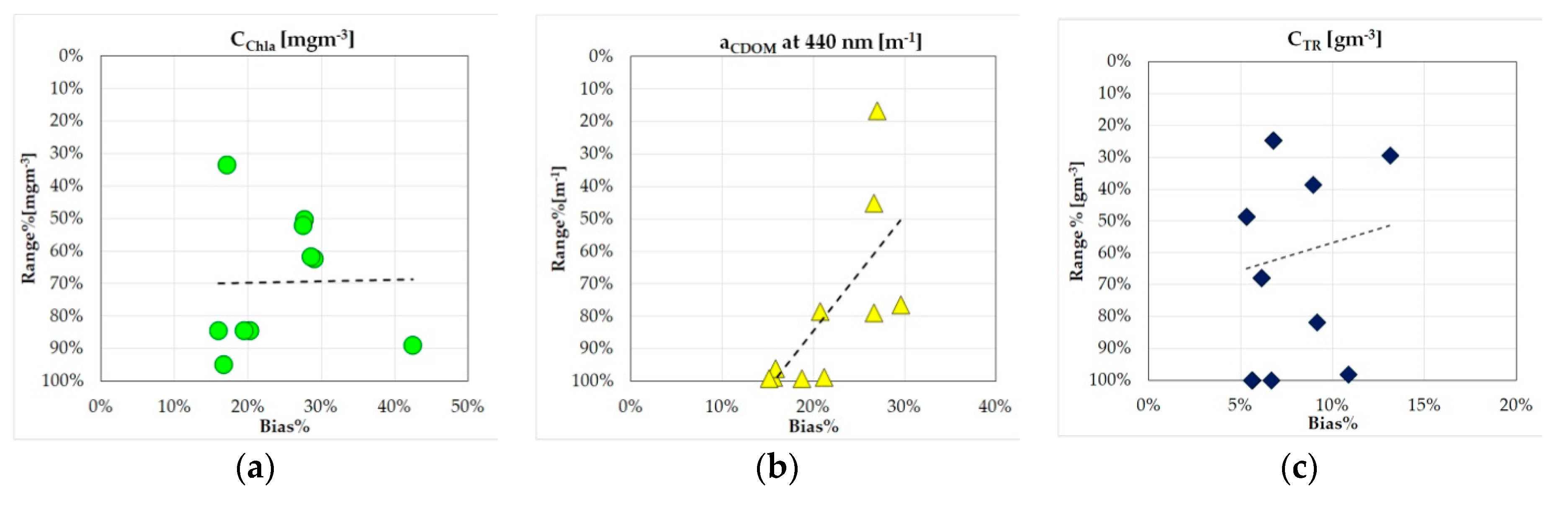Therefore, the results highlighted that the errors in C_Chla, a_CDOM at 440 nm, and C_TR are not only due to the spectral capability of the remote data to resolve their absorption spectra, but also to the characteristics of the coastal waters. To identify these features, the bias% values in C_Chla, a_CDOM at 440 nm, and C_TR retrieved from ASD data using the total bio-optical model were compared with ranges in these water constituents to evaluate their effect on the error. The values taken into consideration were the ranges of each measurement day, the ranges of more measurement days, and total ranges (i.e., 0.09–1.76 mgm⁻³, 0.00–0.41 m⁻¹, and 1.97–8.90 gm⁻³). The relationships between measured ranges in C_Chla, a_CDOM at 440 nm, and C_TR, quantified with the percentages of the range and bias% values in C_Chla, a_CDOM at 440 nm, and C_TR, which were obtained using the total model, are shown in three scatter plots (Figure 8).

These scatter plots highlighted that the range% values in C_Chla, and C_TR, which were measured in situ, are uncorrelated to the bias% values in C_Chla, and C_TR (i.e., the R² values of the best correlation lines are equal to 0.000, and 0.017, respectively), whereas the range% values in a_CDOM at 440 nm seem to be correlated to the bias% values in a_CDOM at 440 nm (i.e., the R² values of the best correlation lines are equal to 0.486). In other words, the errors in a_CDOM at 440 nm seem to increase with the decreasing range in a_CDOM at 440 nm.

4. Discussion

To evaluate the errors in the parametrization of the bio-optical models and to analyze their causes, local, daily, and total bio-optical models were developed; these models and their results were validated, multi- and hyperspectral data were simulated, water constituent concentrations were retrieved from these simulated data, and the results were compared by exploiting the in situ data, which characterized 36 coastal water columns. The validation of local bio-optical models shows a perfect convergence between modeled and measured R_rs (i.e., the mean and standard deviation values of RMS% are equal to 0.1%, and 0.1%, respectively). The mean and standard deviation values of RMS% of the daily and total bio-optical models are equal to 3.8%, 1.7%, and 5.3%, 2.0%, respectively. The values obtained with the total bio-optical model were comparable with the ones evaluated by [15,19]. In fact, the mean and standard deviation values of RMS% described by [15,19] were equal to 5.5%, 1.5%, and 5.1%, 2.0%, respectively. These papers proposed two total bio-optical models for retrieving the water constituents of Venice Lagoon, and Victoria Lake, respectively [15,19]. Therefore, not only the local models, but also the daily and total models adequately retrieved the coastal water constituent concentrations of the Manfredonia Gulf.

The C_Chla, a_CDOM at 440 nm, and C_TR of each column of water were retrieved with local, daily, and total models to validate the results of every model. The differences between the modeled and measured data were evaluated using statistical parameters, which are most useful to assess the capability of a model to resolve the variability of coastal waters, because the attempt to increase accurate knowledge about the spatio-temporal distribution of coastal water constituents represents a crucial challenge [70,71,72]. These statistical parameters and their thresholds were chosen by analyzing the previous papers [12,13,14,15,16,17,18,19,20,67,68]: the best regression line between the modeled and measured data must be close to the 1:1 line [14,15,19], the bias% value must be smaller than 40% [15,19] and the KGE value must be positive [67,68].

With reference to the validation of the model results, every model highlighted a great capability to resolve the variability in the C_Chla, a_CDOM at 440 nm, and C_TR of these coastal waters, because all the best regression lines are close to the 1:1 line, the R² values are greater than 0.54, the bias% values are smaller than 17%, and the KGE values are greater than 0.31. However, the local models possess the greatest capability to resolve the variability of these coastal waters and the daily models possess a greater capability to resolve the variability of these coastal waters than the total model. On the other hand, the mean values of bias% in C_Chla, a_CDOM at 440 nm, and C_TR calculated by the total bio-optical models (i.e., 17%, 15%, and 6%, respectively) were comparable with the ones evaluated by [15,19]. In fact, the mean values of bias% in C_Chla, a_CDOM at 440 nm, and C_TR described by [15] were equal to 15%, 12%, and 9%, respectively. The ones described by [19] were equal to 15%, 9%, and 8%, respectively. Therefore, the validation of the model results confirms that not only the local models, but also the daily and total models can adequately retrieve the coastal water constituents of the Manfredonia Gulf.

After validating the local, daily, and total models and their results, these bio-optical models were applied to CHRIS mode 1 and mode 2, Landsat TM, MIVIS, MODIS, and PRISMA simulated data. The first important outcome of these applications is that every model applied to CHRIS mode 1 and mode 2, MIVIS, MODIS, and PRISMA data adequately resolves the variability in C_TR and their errors in C_TR are comparable. The Landsat TM data highlighted the worst capability to retrieve C_TR (i.e., slope of the best regression line equal to 0.62 and R², bias%, and KGE values equal to 0.46, 20%, and 0.66, respectively). However, the PRISMA data highlighted the best capability to retrieve C_TR (i.e., slope of the best regression line equal to 0.72 and R², bias%, and KGE values equal to 0.89, 11%, and 0.73, respectively). In conclusion, the C_TR retrieved from all data using the total model meet the chosen requirements and these results can be taken into consideration. Errors in C_TR (i.e., R², bias%, and KGE values) obtained from all datasets using the total models are equal to 0.90, 10%, and 0.75 gm⁻³, 0.85, 10%, and 0.75 gm⁻³, 0.46, 20%, and 0.66 gm⁻³, 0.88, 8%, and 0.83 gm⁻³, 0.67, 14%, and 0.70 gm⁻³, and 0.89, 11%, and 0.73 gm⁻³, respectively. This outcome is very important because the total bio-optical model allows us to adequately retrieve the C_TR of Manfredonia Gulf from remote data that were not acquired at the same time as in situ surveys (Table 1). Therefore, it is possible to exploit the spatial and spectral resolutions of CHRIS mode 2 data, the spatial resolutions of the Landsat TM data, and the temporal resolutions of the MODIS data, all of which were not simultaneously acquired with respect to the in situ data (Table 1). These applications also provide an uncertainty assessment of these remote data: uncertainties in C_TR due to the application of the total model to CHRIS mode 2, Landasat TM, and MODIS data are equal to ± 0.99 gm⁻³, ± 1.84 gm⁻³, and ± 1.38 gm⁻³, respectively. Moreover, merging the results of these simultaneous images allows us to minimize the error and increase the spatial resolution [73]. With reference to images simultaneously acquired with respect to in situ data (Table 1), the application of the local or daily models, rather than the total model, to retrieve C_TR allows to minimize errors. Moreover, merging these results also minimizes the error and increases the spatial resolution [73].

The second important outcome of these applications is that the results of daily and total models, which were applied to CHRIS mode 1 and mode 2, MIVIS, and MODIS data do not meet the requirements for adequately characterizing the variability in C_Chla, and a_CDOM at 440 nm. In other words, only local bio-optical models can adequately retrieve C_Chla, and a_CDOM at 440 nm of the coastal waters from these data. This means that only the remote images, which were simultaneously acquired with respect to in the situ data, can be used and, before applying the local models, these images have to be divided into many zones which have to be quasi “co-located” with respect to in situ data. Moreover, the results of every model applied to the Landsat TM data do not meet the requirements for adequately characterizing the variability in C_Chla, and a_CDOM at 440 nm. Therefore, no image acquired by the Landsat TM sensor during the campaign can be used to adequately retrieve the C_Chla and a_CDOM at 440 nm in these coastal waters.

The third important outcome of these applications is that the total models resolve the variability in C_Chla using PRISMA data (i.e., slope of the best regression line equal to 0.76 and R², bias%, and KGE values equal to 0.38, 22%, and 0.51, respectively) and that the total models poorly resolve the variability in a_CDOM at 440 nm using PRISMA data (i.e., slope of the best regression line equal to 0.88 and R², bias%, and KGE values equal to 0.35, 34%, and −0.51, respectively).

As the local bio-optical model is only applied to remote data that is “simultaneous and co-located” with respect to in situ data that were used to develop and validate this model and their results, the results confirm that “simultaneous and co-located” data minimize the error in the retrieval of water constituent concentrations [3,5,6,7,9,11]. On the other hand, as only the total models take full advantage of the spatial and temporal resolutions of the remote data, most of the previous works have proposed total bio-optical models for retrieving coastal and inland water constituent concentrations [12,13,14,15,16,17,18,19,20], a few papers have proposed daily ones [14,15], and none of the authors proposed local ones. The literature highlighted that the spectral capability of remote images to retrieve the concentrations of coastal and inland water constituents is another source of significant errors in their monitoring [3,5,12,13,14,15,16,17,18,19,20,21,22]. To prove that the error in the choice of the model type is closely related to the spectral capability of remote images to resolve the absorption spectra of coastal water constituents, multi- and hyperspectral data were taken into consideration. The differences between the modeled and measured R_rs spectra used to validate the models only provides overall information on the errors in C_Chla, a_CDOM at 440 nm, and C_TR and give no information on the errors in every single constituent. As IPOs vary only according to the composition of the medium or constituents [3,4,5,6], these spectra were used to assess the spectral capabilities of the sensors to characterize the coastal water of Manfredonia Gulf. In other words, the spectrally resampled absorption spectra used as inputs into the local, daily, and total models that were applied to these data were compared with the IPOs spectra measured in situ (called the starting absorption spectra). Their differences were calculated to evaluate the spectral capabilities of the selected remote data to resolve the absorption spectra. The results (i.e., RMS%^ab values) provide the order of these sensors according to these differences and this order is comparable with the order of the same sensors according to the errors in C_Chla, a_CDOM at 440 nm, and C_TR. Therefore, PRISMA data obtained the smallest RMS%^ab values in a_Chla, a_CDOM, and a_TR and these data are able to adequately retrieve the variability in C_Chla, a_CDOM at 440 nm, and the C_TR of these coastal waters using the total model. However, the Landsat TM data obtained the greatest RMS%^ab values in a_Chla, a_CDOM, and a_TR and these data cannot adequately retrieve the variability in C_Chla, and a_CDOM at 440 nm of these coastal waters, whereas these data are able to adequately retrieve the variability in C_TR using the total model.

All remote data that could not adequately resolve the variability in C_Chla using the local, daily, and total models highlighted RMS%^ab values that were evaluated by comparing a_Chla greater than 23.58% (i.e., RMS%^ab values calculated from MODIS data using the local models); all remote data that could not adequately resolve the variability in a_CDOM at 440 nm using local, daily, total models highlighted RMS%^ab values that were evaluated by comparing a_CDOM greater than 7.67% (i.e., RMS%^ab values calculated from PRISMA data using the total model), except MIVIS data. This sensor does not acquire the first wavelengths of the analyzed spectral range (i.e., the first band is at 442 nm with a spectral resolution of 21.1 nm). RMS%^ab values obtained by comparing a_TR are smaller than 9.73% (i.e., RMS%^ab values calculated from Landsat TM data using the total model) and an error analysis highlighted that every sensor was able to adequately resolve the variability in the C_TR of these coastal waters. In conclusion, one very important outcome of this evaluation is that RMS%^ab values seemed to identify the threshold between the data that adequately characterized these coastal waters and the data that could not adequately characterize them. In other words, the threshold can help to parametrize the bio-optical models and assist in the choice between the local, daily, and total ones.

The comparison of RMS%^ab values and the errors showed that RMS%^ab values evaluated using a_CDOM are smaller than those obtained using a_Chla, whereas the errors in a_CDOM at 440 nm are greater than the ones in C_Chla. Therefore, the errors were compared with range of water constituent concentrations measured in situ. C_Chla, a_CDOM440nm, and C_TR varied from 0.09 to 1.76 mgm⁻³, from 0.00 to 0.41 m⁻¹, and from 1.97 to 8.90 gm⁻³. The ranges of each measurement day, two measurement days, three measurement days, and all measurement days were compared with the mean values of the errors in C_Chla, a_CDOM at 440 nm, and C_TR, which were obtained using the total model. The relationships between the errors and their ranges highlighted that the errors in a_CDOM440nm slightly increased as the range decreased. However, the ranges in C_Chla, and C_TR were uncorrelated compared to the errors in C_Chla and C_TR. One important outcome of these comparisons is that, in waters where the water constituent concentration range is small, the error in the parametrization of the bio-optical models is closely related not only to the spectral capability of the remote data to resolve the absorption spectra, but also to the abundance of water constituent concentrations. The water constituent concentrations and the developed bio-optical models previously proposed confirm this outcome [e.g., 15,19]. Cavalli et al. [19] proposed a total model for retrieving the water constituents of Victoria Lake only using absorption and backscattering spectra as inputs, which were sourced from the literature. The concentration range of every water constituent that was monitored was very large. C_Chla, a_CDOM440nm, and C_TR measured in situ varied from 6.6 to 29.1 mgm⁻³, from 1.2 to 8.1 m⁻¹, and from 87 to 433 gm⁻³, respectively [19]. However, Santini et al. [15] proposed a daily model for retrieving the water constituents of Venice Lagoon using absorption spectra, which were simultaneously acquired with respect to remote data, as inputs. The concentration range of water constituents were larger than those of the coastal waters of Manfredonia Gulf. C_Chla, a_CDOM440nm, and C_TR measured in situ varied from 0.41 to 10.11 mgm⁻³, from 0.19 to 0.54 m⁻¹, and from 2.72 to 20.17 gm⁻³, respectively [19]. Therefore, the total bio-optical model adequately retrieves water constituent concentrations where their range is large, and vice versa—the local bio-optical models adequately retrieve water constituent concentrations where their range is small.

5. Conclusions

The main challenge of bio-optical models is to fully exploit the spatial and temporal resolutions of remote images by developing models that better resolve the total spatial and temporal variability of coastal waters (i.e., total models). However, to improve the thematic accuracy of image products, the model should fully resolve the local variability (i.e., local model) using absorption spectra that are “simultaneous and co-located”, with respect to remote images, as inputs. To evaluate the errors in the parametrization of the bio-optical models, in situ data acquired in the coastal waters of Manfredonia Gulf were used to develop 36 local models, four daily models, and one total bio-optical model to validate each of the models and their results. Therefore, these models were applied to CHRIS mode 1 and mode 2, Landsat TM, MIVIS, MODIS, and PRISMA simulated data for retrieving water constituent concentrations. The comparison of these data highlighted that errors in coastal water constituent concentrations decrease considerably when using the local models compared to the total model, and they slightly decrease when using the daily models compared to the total model.

However, the results highlighted that some remote data are able to adequately retrieve the coastal water constituent concentrations using total or daily bio-optical models, while others are not able to do this. In any case, evaluating the errors in the parametrization of bio-optical models and knowing their causes are crucial before persisting in developing bio-optical models or changing or merging methods and/or data.

To understand these results, the capability of the selected remote data to resolve the absorption spectra of the water constituents was evaluated by calculating the differences between the measured and spectrally resampled absorption spectra. The resultant capabilities were compared with the errors in water constituent concentrations and they were well correlated, except for the errors in the absorption of the colored dissolved organic material at 440 nm. Therefore, the ranges of the measured water constituent concentrations were compared with their errors, which were retrieved using the total bio-optical model. However, the ranges of chlorophyll-a and tripton particle concentrations did not correlate with their errors, while the errors in the absorption of the colored dissolved organic material at 440 nm did correlate with their abundance. The data of the previous proposed models, which were compared with these results, confirm this important outcome.

Therefore, this paper proves that, in coastal and inland waters characterized by a great abundance of water constituents, the errors in the parametrization the bio-optical models are principally due to the spectral capability of remote images to resolve the absorption spectra of the water constituents. On the contrary, in coastal and inland waters characterized by a small abundance of water constituents, the errors in the parametrization of the bio-optical models is due not only to the spectral capability of remote images to resolve the absorption spectra of the water constituents, but also to the range of water constituent concentrations.

One the one hand, this paper confirms that the use of local bio-optical models minimizes the error in the retrieval of coastal water constituents by evaluating and comparing the errors caused by the application of local, daily, and total models. On the other hand, this paper demonstrates that not only the spectral capability of remote images to resolve the absorption spectra, but also an analysis of the range of coastal water constituent concentrations allow to lead the choice in the parameterization of bio-optical models minimiziong the errors in the retrieval of coastal water constituents.