A Virtual Geostationary Ocean Color Sensor to Analyze the Coastal Optical Variability

 , ,
, ,
Abstract
:
1. Introduction
- (a)
- Be univariate (i.e., with multiple images of the same parameter only).
- (b)
- Contain a set of time slices, all of which must be precisely coregistered (with image-to-image pixels perfectly aligned spatially).
- (c)
- Exhibit radiometric consistency between images (i.e., they are measured using the same sensors or inter-validated sensor systems, and exhibit a degree of normalization between time slices).
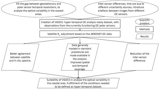
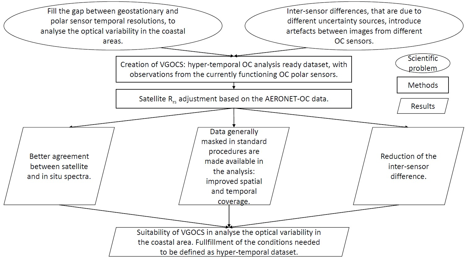
- The suitability of VGOCS in analyzing the coastal optical variability, by the study of the effect of the adjustment on the quality of the satellite data, the VGOCS spatial and temporal coverage, and the intersensor differences.
- The fulfillment of the three conditions for a hyper-temporal dataset [29].
2. Materials and Methods
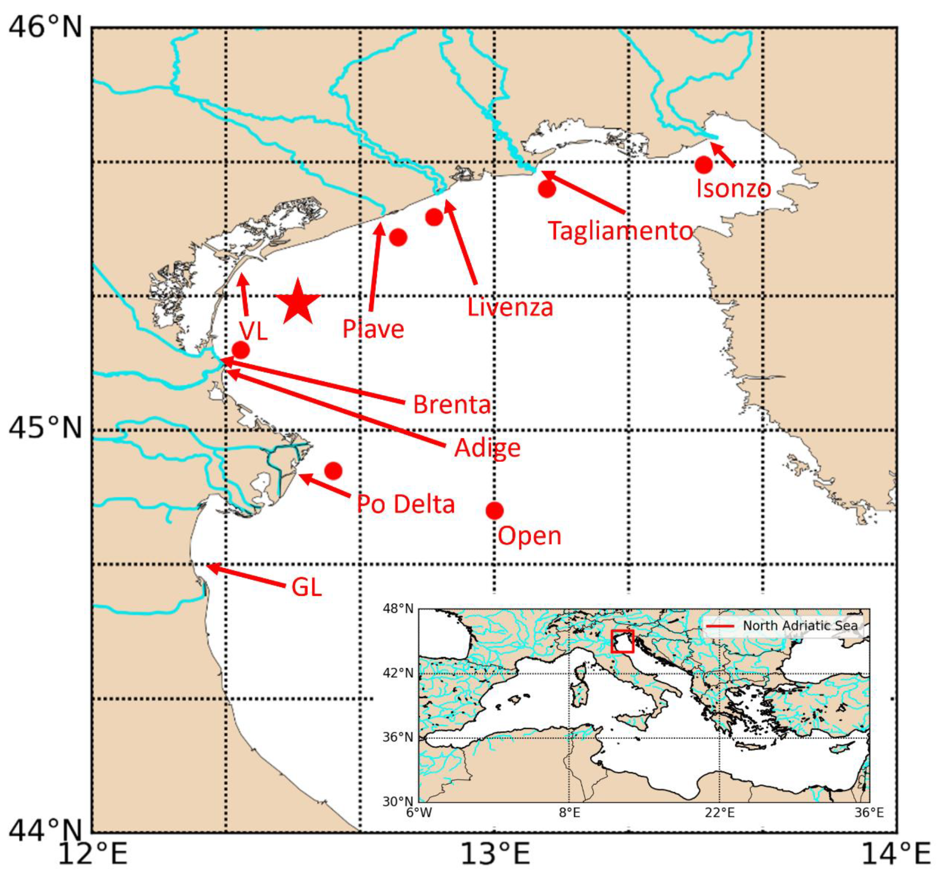
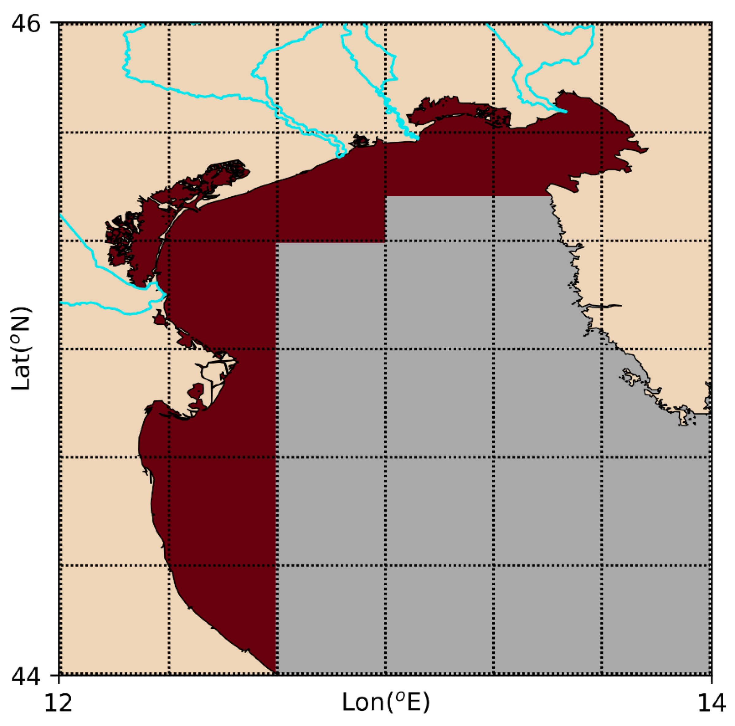
2.1. Study Area
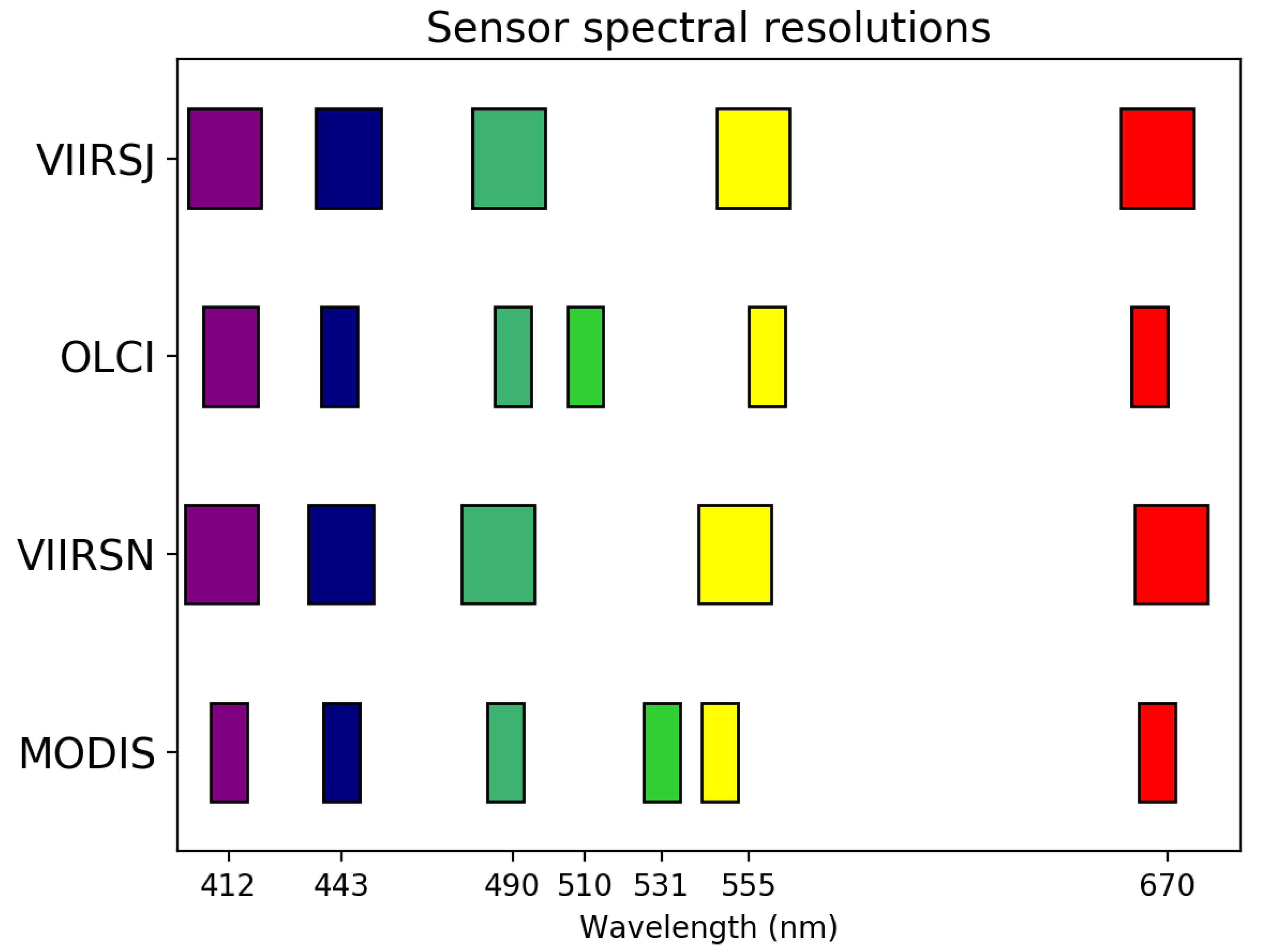
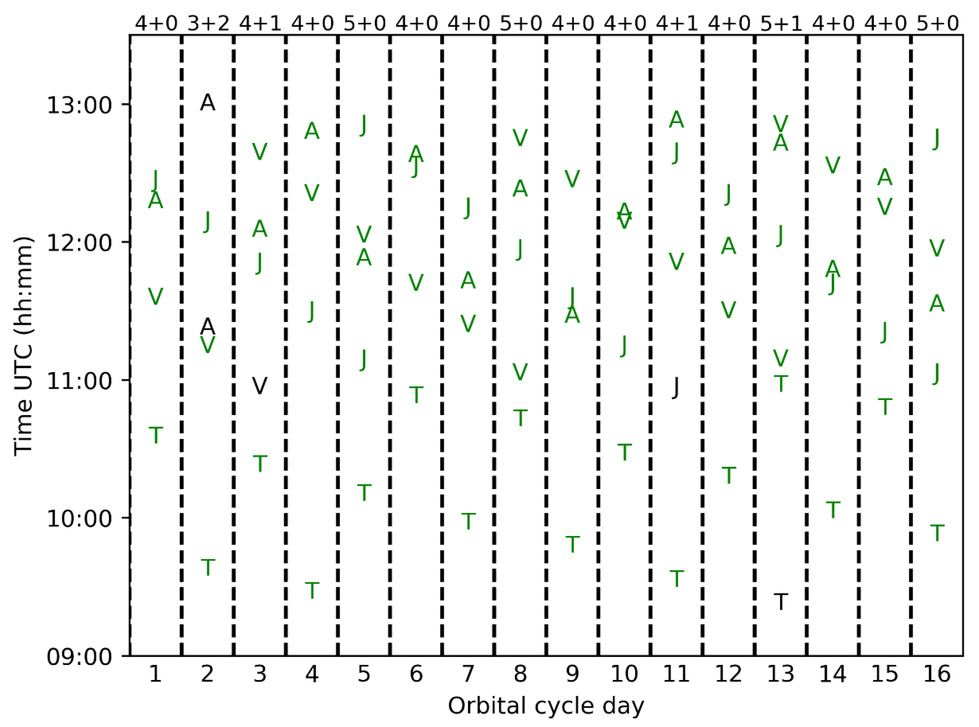
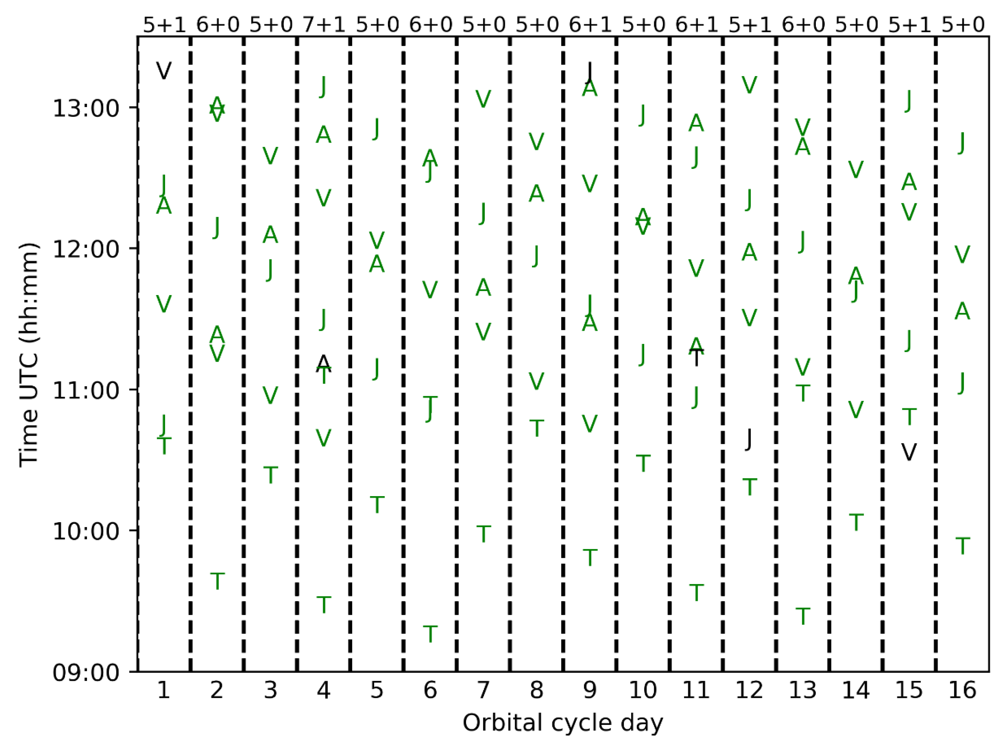
2.2. VGOCS Sensors
- The NASA Moderate-Resolution Imaging Spectroradiometer (MODIS) sensors mounted on the AQUA and TERRA satellites, here simply referred to as AQUA and TERRA respectively.
- The National Oceanic and Atmospheric Administration (NOAA) VIIRS sensors mounted on the SUOMI-NPP and NOOA-20 (previously JPSS-1) satellites, here referred to as VIIRSN and VIIRSJ respectively.
- The European Space Agency (ESA)/EUMETSAT Ocean and Land Color Instrument (OLCI) mounted on Sentinel 3A, here referred simply as OLCI.
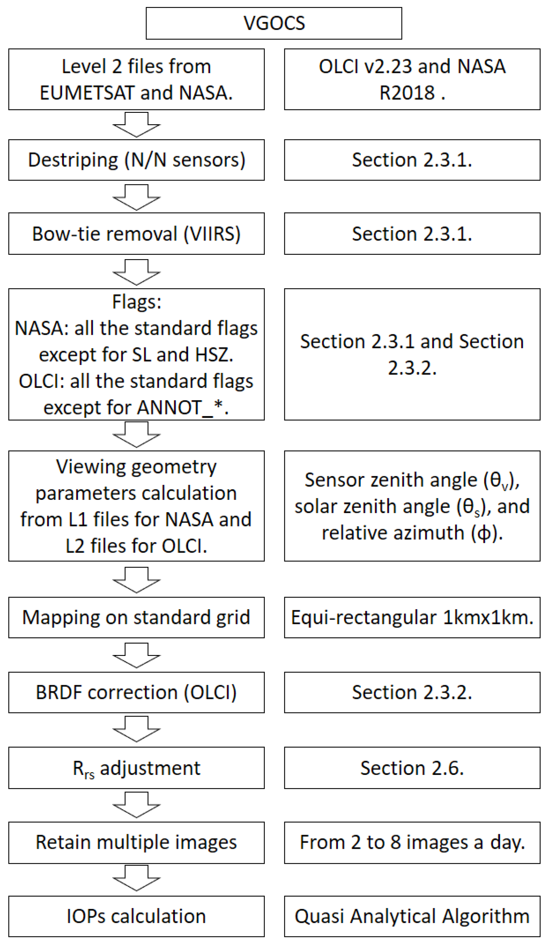
2.3. VGOCS Dataset and Processing Chain
- The Rrs_data group, where the Rrs spectra at the native sensor resolution are stored.
- The IOP_data group, where all the parameters (listed below) calculated with the QAA can be found [34,35]:
- ○
- reference wavelength (λ0)
- ○
- total absorption at the reference wavelength (a(λ0))
- ○
- particulate backscattering at the reference wavelength (bbp(λ0))
- ○
- bbp spectral slope (η)
- ○
- bbp at 443 nm (bbp(443))
- ○
- absorption by nonalgal particles and dissolved matter at 443 nm (adg(443))
- ○
- adg spectral slope (s)
- ○
- absorption by phytoplankton at 443 nm (aphy(443))
- The Atmospheric_data group contains some atmospheric parameters, such as aerosol optical thickness and angstrom coefficients, extracted from the L2 files.
- The Geo_data group contains information about the applied flags, extracted from the L2 files, and about some viewing geometry parameters, such as the sensor zenith angle (θv), the solar zenith angle (θs), and the relative angle between the solar and sensor azimuth angle (φ). Those parameters for the OLCI sensor are extracted from the L2 file, for the VIIRS sensors from the L1 GEO files, while for the MODIS sensors they are retrieved using the L1B files as the input of l2gen.
2.3.1. NASA/NOAA Sensors
- For VIIRSN there are 9 full orbit overlaps in comparison with the two available maskings for HSZ.
- For VIIRSJ there are 8 full and 2 partial overlaps in comparison with the two available maskings for HSZ.
- For AQUA and TERRA, there are 3 full orbit overlaps (previously zero), and some additional partial images.
2.3.2. OLCI Sensor
2.4. In Situ Data
2.5. Match-up Analyses
2.6. Satellite Rrs Adjustment
2.7. Inter-Sensor Differences
- At AAOT, to analyze the effect of the adjustment in an area with large optical variability.
- Close to the Livenza, Brenta-Adige, Piave, Tagliamento, and Isonzo river mouths to analyze the effect of the adjustment in optically complex waters.
- In an off-shore location (here named simply OPEN), to analyze the effect of the adjustment in open waters.
3. Results
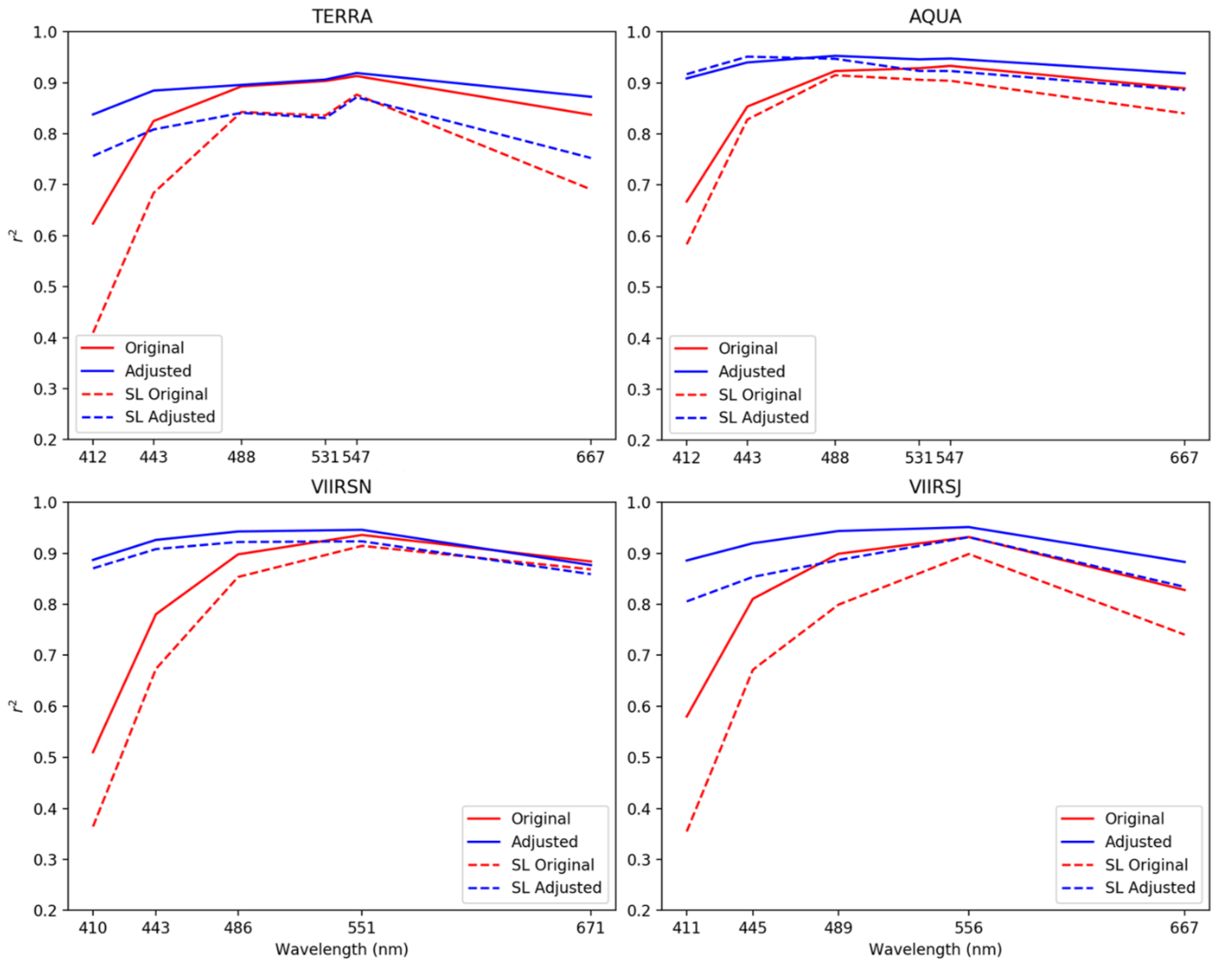
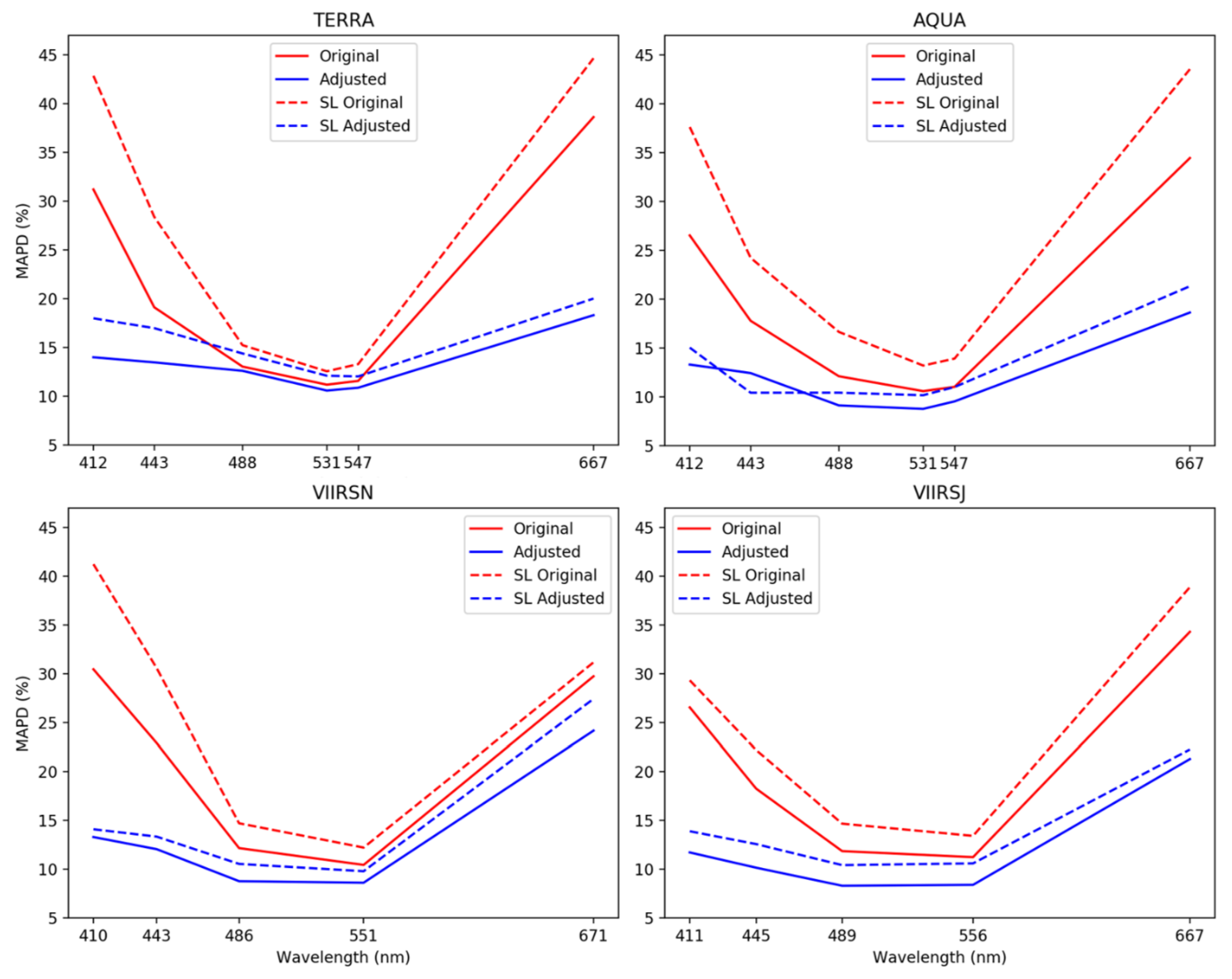
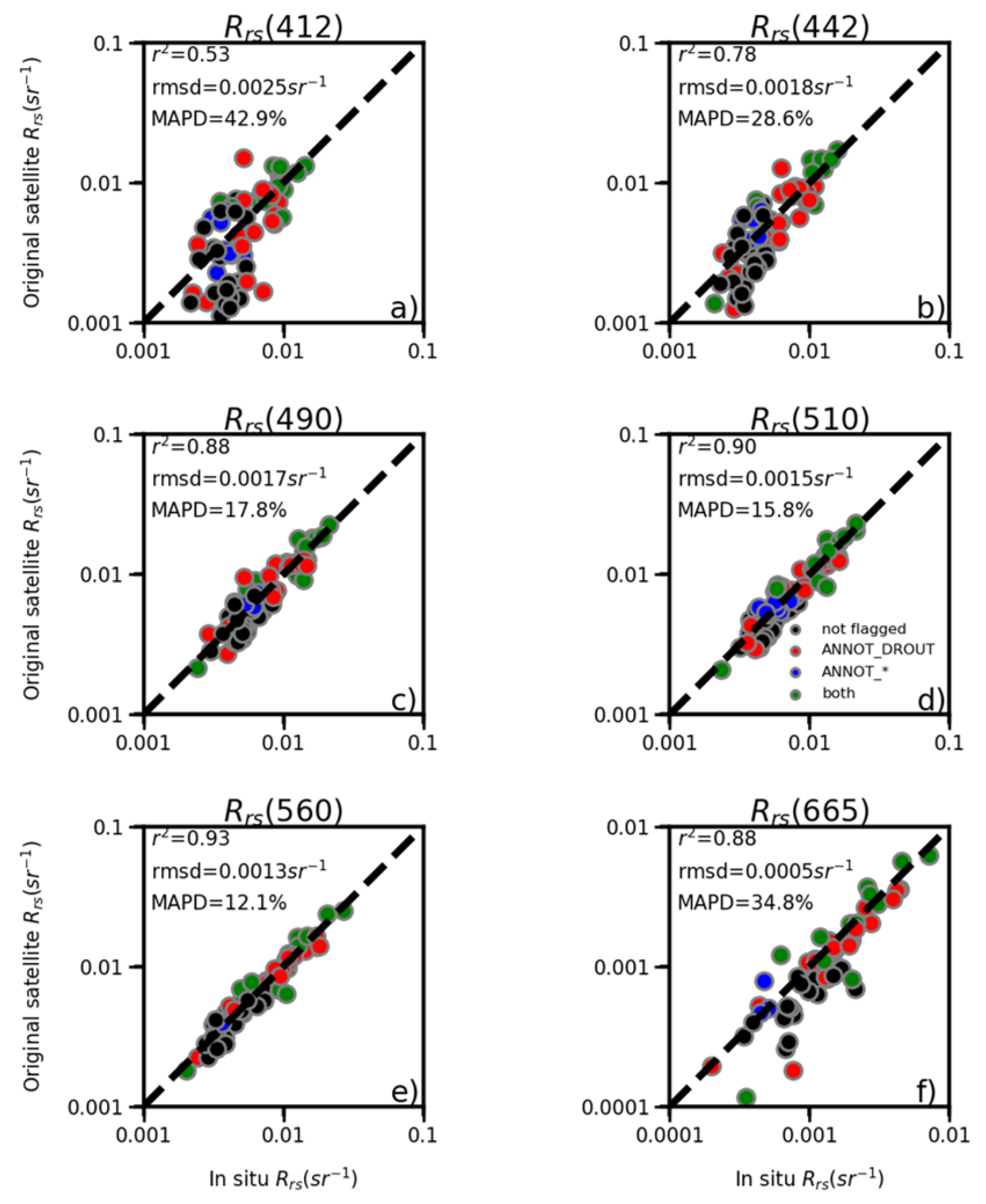
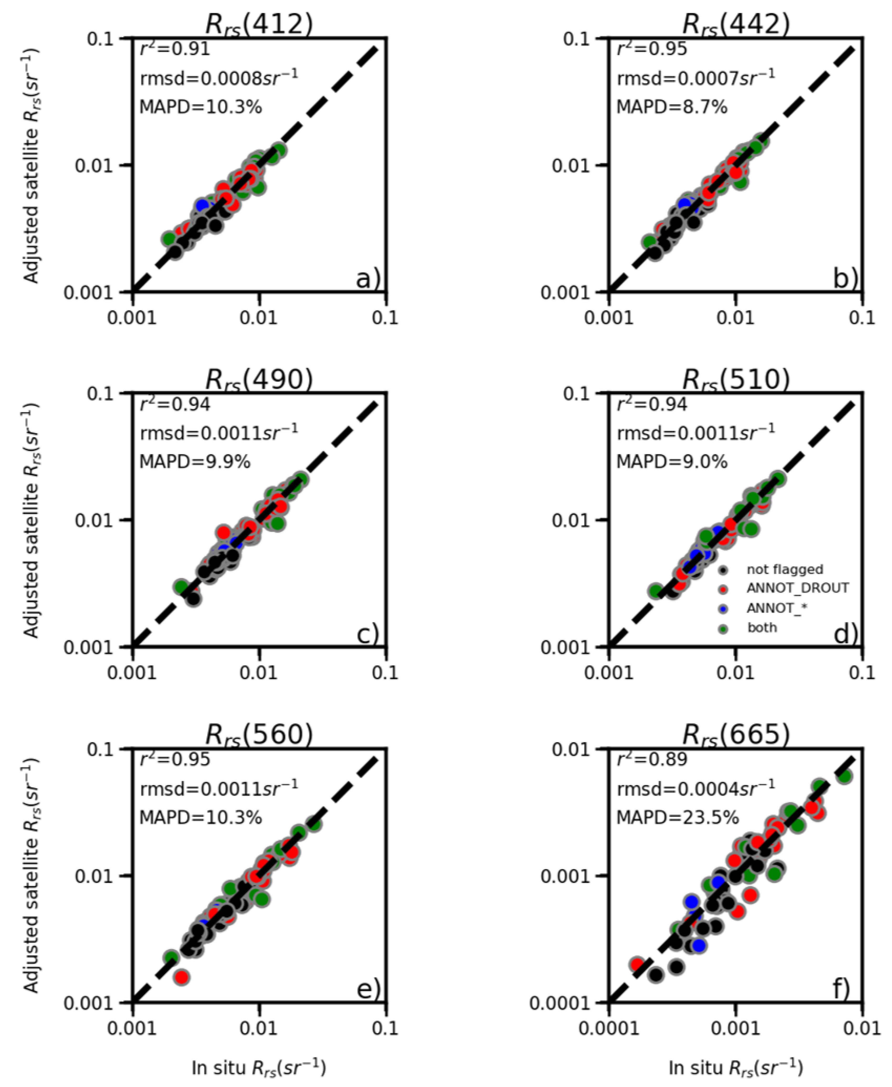
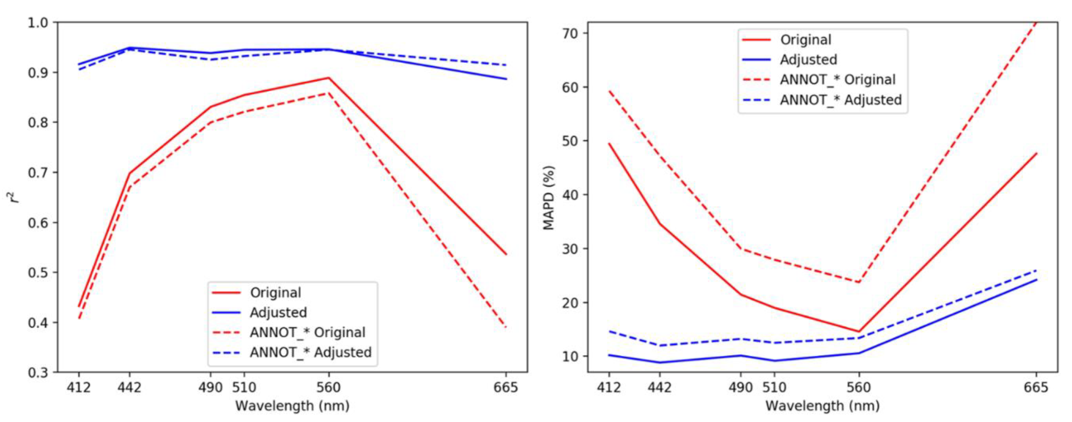
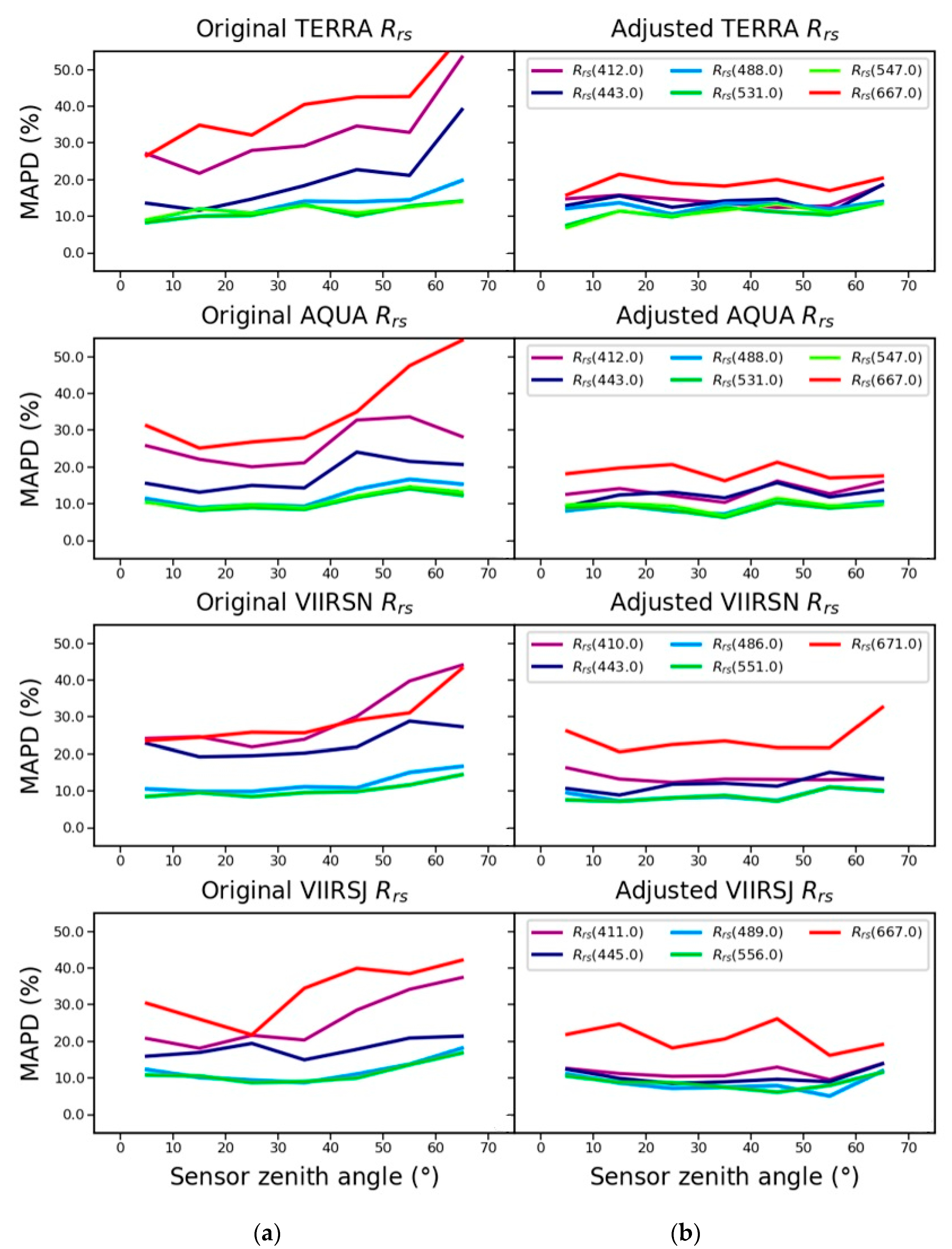
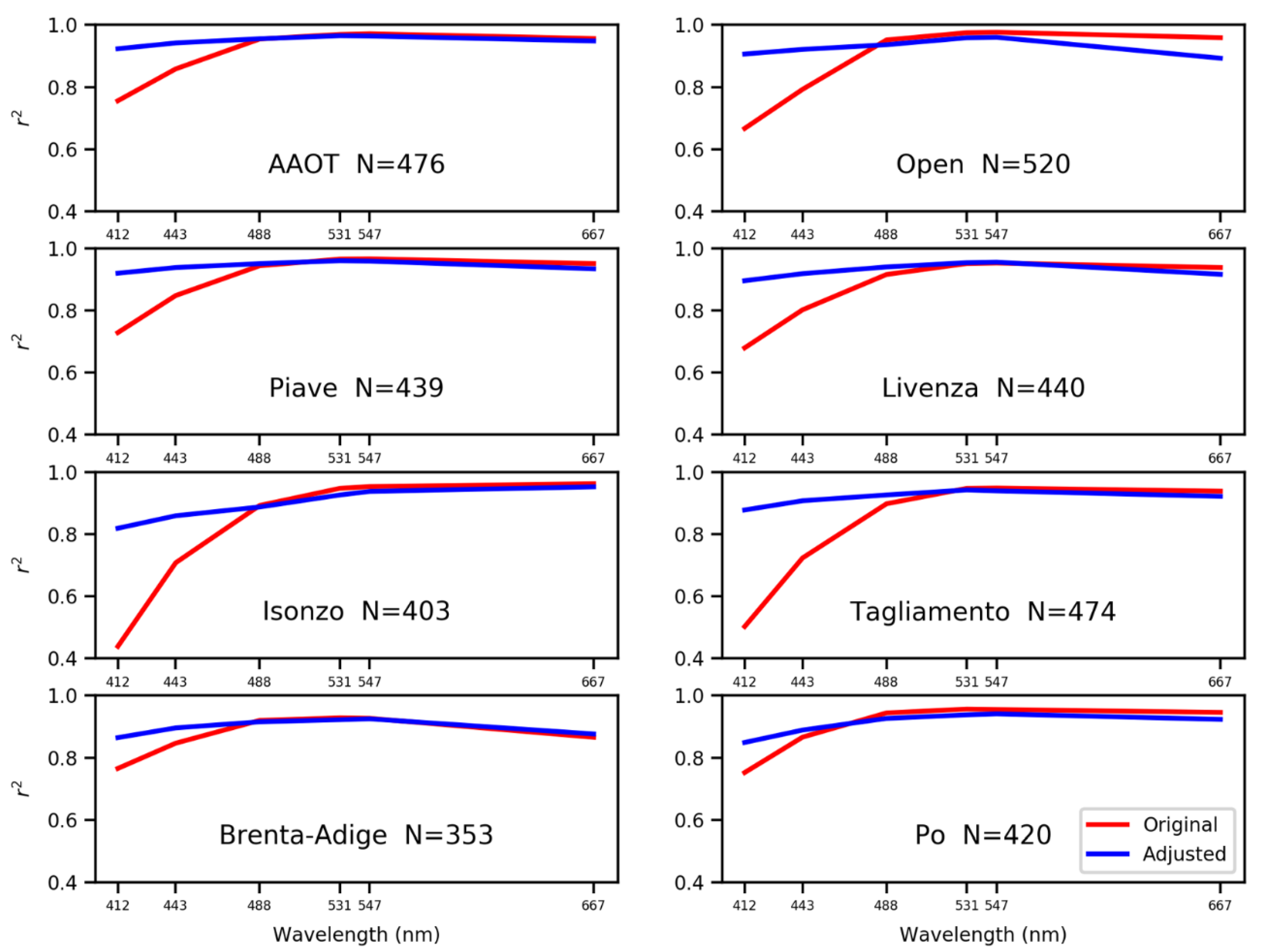
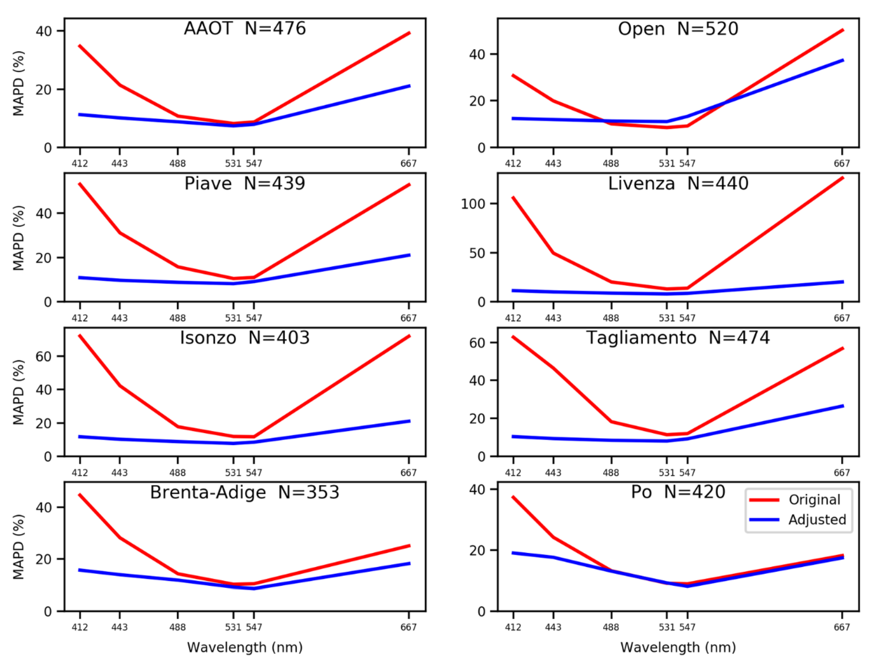
3.1. Match-Up Analyses
3.2. VGCOS Spatial and Temporal Coverage
3.2.1. HSZ Flag
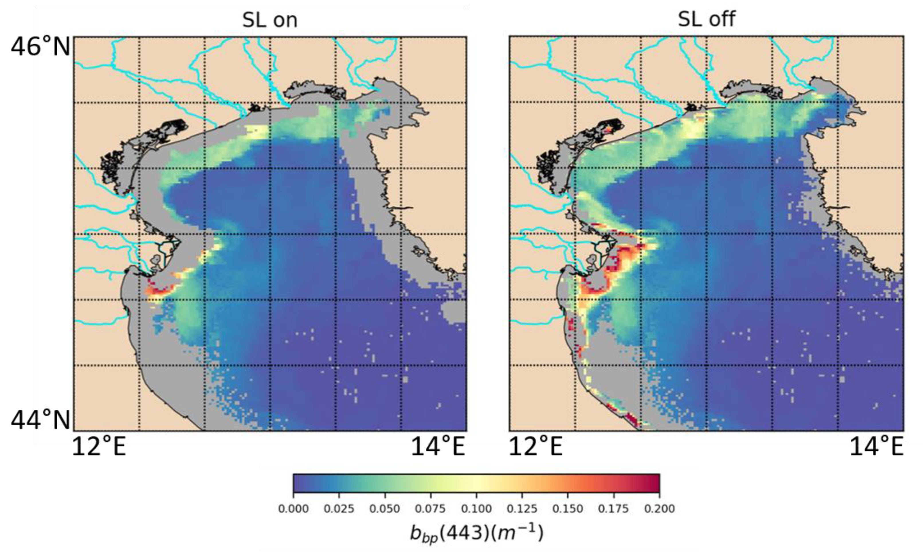
3.2.2. SL Flag
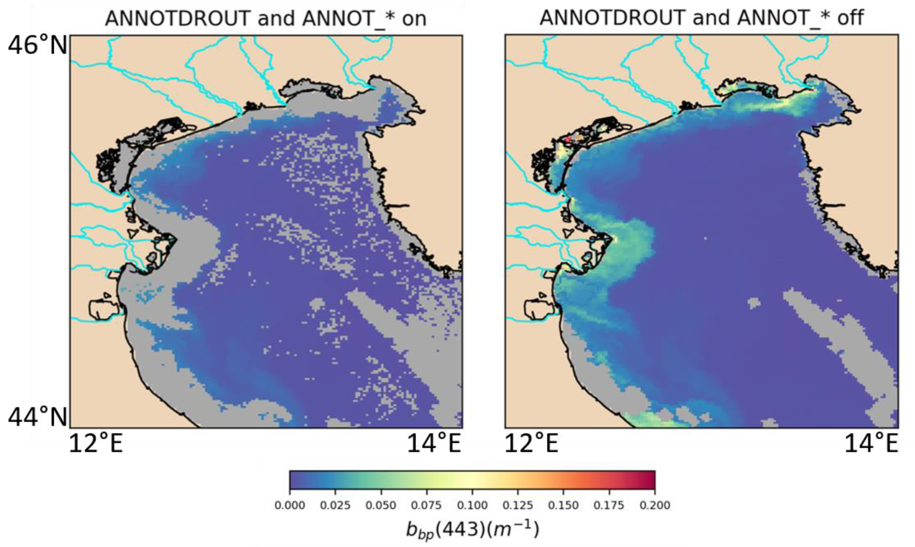
3.2.3. ANNOT_DROUT and ANNOT_* Flags
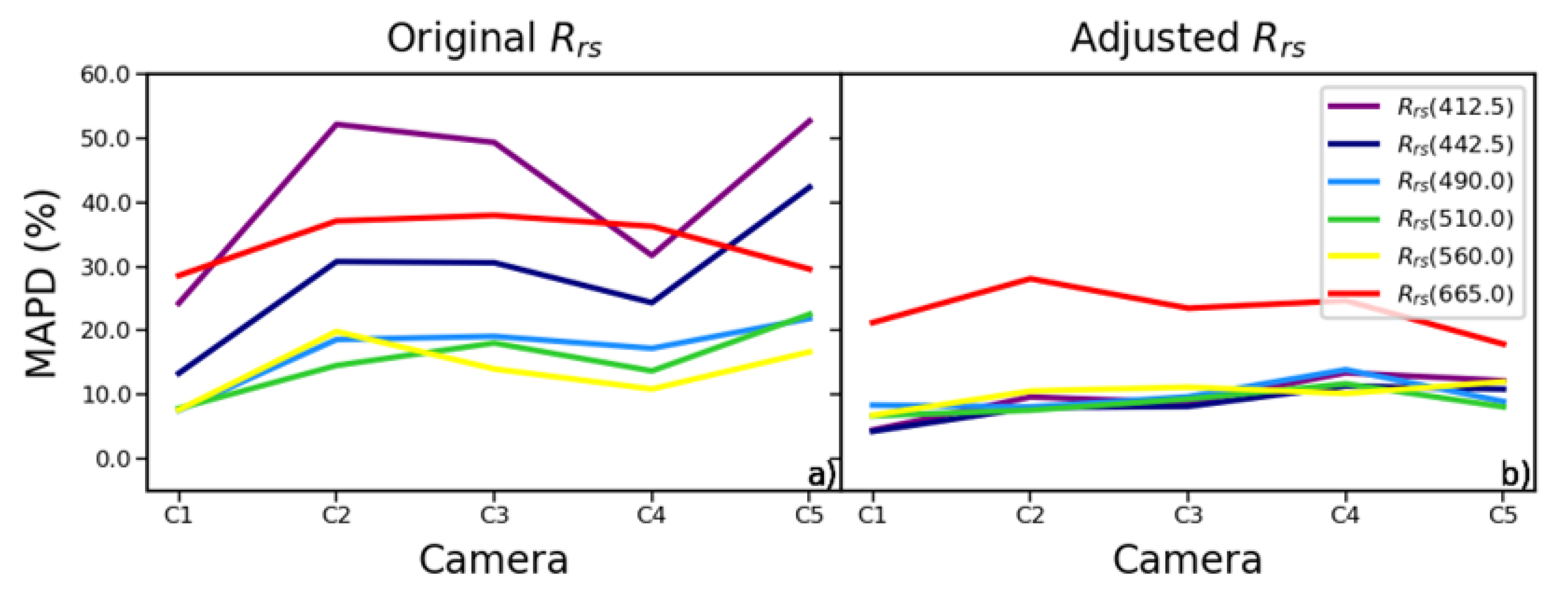
3.3. OLCI Camera Dependence
3.4. Inter-Sensor Differences
4. Discussion
- (a)
- The variables stored in the dataset must be univariate. As the Rrs data are provided at their native spectral resolution to reduce the uncertainty in the band-shifting procedure, the variables stored in the Rrs_data group are different for each sensor and this condition seems to be not fulfilled. Nevertheless, the Rrs data group is mainly provided for post-processing procedures and it allows the users to calculate different IOPs and water component concentrations using different algorithms [92,93,94,95]. The parameters that are needed to analyze the coastal optical variability, the aim for which VGOCS is conceived, are the IOPs, that are the same for each sensor, fulfilling the first requirement.
- (b)
- All the images must be time referenced and the same grid should be used for each image of the dataset. This is fulfilled because the name of each file gives information about the acquisition time, and each image of the dataset is reprojected on a standard 1 km × 1 km equirectangular grid.
- (c)
- All the sensors must be inter-validated between each other. This condition is also reached, as they are all adjusted on the AERONET-OC AAOT in situ data and the adjustment significantly reduced the inter-sensor differences.
5. Conclusions
- The Western Black Sea where the Gloria, Section-7, and Galata Platform AERONET-OC stations are present [96].
- In the Northern Sea where the Zeebrugge-MOW1 and Thornton_C-Power, part of the AERONET-OC network, are located [97].
- In the Baltic Sea where the Helsinki Lighthouse, Irbe Lighthouse, and Gustav Dalen Tower AERONET-OC stations are present [19]. As this basin is located at higher latitudes than the NAS, the satellite overpasses above such area are more frequent, making the approach also more powerful. Nevertheless, due to a large amount of CDOM present in these waters [98], a different atmospheric correction is needed to retrieve reliable Rrs spectra [99,100,101].
- The North-Western Mediterranean where the BOUee pour l’aquiSition d’une Serie Optique a Long termE mooring (BOUSSOLE) [102] and the Casablanca AERONET-OC [103] station are located. Particularly, BOUSSOLE has been used for the system vicarious calibration of the OLCI sensor [104]; hence, it could be interesting to test the effect of the adjustment using such data as input of the MLR algorithm.
- The areas where the different WATERHYPERNET network sites are located [105]. This network, which will be developed in the next years, is based on the concept of AERONET-OC [26], but with the essential advantage of the exploitation of a hyperspectral radiometer [106]. The use of such an instrument will allow validating each band of each satellite mission [106], reducing the uncertainties that could be introduced by band-shifting procedures [88,107].
Author Contributions
Funding
Acknowledgments
Conflicts of Interest
References
- IOCCG. Why Ocean Colour? The Societal Benefits of Ocean-Colour Technology; Reports of the International Ocean-Colour Coordinating Group, No. 7; IOCCG: Bedford, NS, Canada, 2008. [Google Scholar]
- IOCCG. Mission Requirements for Future Ocean-Colour Sensors; Reports of the International Ocean-Colour Coordinating Group, No. 13; IOCCG: Bedford, NS, Canada, 2012. [Google Scholar]
- McClain, C.R.; Meister, G.; Monosmith, B. Satellite Ocean Color Sensor Design Concepts and Performance Requirements. In Experimental Methods in the Physical Sciences; Academic Press: Cambridge, MA, USA, 2014; Volume 47, pp. 73–119. [Google Scholar]
- Mouw, C.B.; Greb, S.; Aurin, D.; DiGiacomo, P.M.; Lee, Z.; Twardowski, M.; Binding, C.; Hu, C.; Ma, R.; Moore, T.; et al. Aquatic color radiometry remote sensing of coastal and inland waters: Challenges and recommendations for future satellite missions. Remote Sens. Environ. 2015, 160, 15–30. [Google Scholar] [CrossRef]
- Arnone, R.A.; Vandermeulen, R.A.; Soto, I.M.; Ladner, S.D.; Ondrusek, M.E.; Yang, H. Diurnal changes in ocean color sensed in satellite imagery. J. Appl. Remote Sens. 2017, 11, 032406. [Google Scholar] [CrossRef] [Green Version]
- Bracaglia, M.; Volpe, G.; Colella, S.; Santoleri, R.; Braga, F.; Brando, V.E. Using overlapping VIIRS scenes to observe short term variations in particulate matter in the coastal environment. Remote Sens. Environ. 2019, 233, 111367. [Google Scholar] [CrossRef]
- Chen, Z.; Hu, C.; Muller-Karger, F.E.; Luther, M.E. Short-term variability of suspended sediment and phytoplankton in Tampa Bay, Florida: Observations from a coastal oceanographic tower and ocean color satellites. Estuar. Coast. Shelf Sci. 2010, 89, 62–72. [Google Scholar] [CrossRef]
- Qi, L.; Hu, C.; Barnes, B.B.; Lee, Z. VIIRS captures phytoplankton vertical migration in the NE Gulf of Mexico. Harmful Algae 2017, 66, 40–46. [Google Scholar] [CrossRef]
- Choi, J.K.; Park, Y.J.; Ahn, J.H.; Lim, H.S.; Eom, J.; Ryu, J.H. GOCI, the world’s first geostationary ocean color observation satellite, for the monitoring of temporal variability in coastal water turbidity. J. Geophys. Res. Ocean. 2012, 117. [Google Scholar] [CrossRef]
- Lavigne, H.; Ruddick, K. The potential use of geostationary MTG/FCI to retrieve chlorophyll-a concentration at high temporal resolution for the open oceans. Int. J. Remote Sens. 2018, 39, 2399–2420. [Google Scholar] [CrossRef]
- Neukermans, G.; Ruddick, K.; Bernard, E.; Ramon, D.; Nechad, B.; Deschamps, P.Y. Mapping total suspended matter from geostationary satellites: A feasibility study with SEVIRI in the Southern North Sea. Opt. Express 2009, 17, 14029–14052. [Google Scholar] [CrossRef] [Green Version]
- Choi, J.K.; Park, Y.J.; Lee, B.R.; Eom, J.; Moon, J.E.; Ryu, J.H. Application of the Geostationary Ocean Color Imager (GOCI) to mapping the temporal dynamics of coastal water turbidity. Remote Sens. Environ. 2014, 146, 24–35. [Google Scholar] [CrossRef]
- Concha, J.; Mannino, A.; Franz, B.; Kim, W. Uncertainties in the Geostationary Ocean Color Imager (GOCI) Remote Sensing Reflectance for Assessing Diurnal Variability of Biogeochemical Processes. Remote Sens. 2019, 11, 295. [Google Scholar] [CrossRef] [Green Version]
- Ruddick, K.; Neukermans, G.; Vanhellemont, Q.; Jolivet, D. Challenges and opportunities for geostationary ocean colour remote sensing of regional seas: A review of recent results. Remote Sens. Environ. 2014, 146, 63–76. [Google Scholar] [CrossRef] [Green Version]
- Wang, M.; Son, S.; Jiang, L.; Shi, W. Observations of ocean diurnal variations from the Korean geostationary ocean color imager (GOCI). In Ocean Sensing and Monitoring VI; International Society for Optics and Photonics: Bellingham, WA, USA, 2014; Volume 9111, p. 911102. [Google Scholar]
- Ryu, J.H.; Han, H.J.; Cho, S.; Park, Y.J.; Ahn, Y.H. Overview of geostationary ocean color imager (GOCI) and GOCI data processing system (GDPS). Ocean Sci. J. 2012, 47, 223–233. [Google Scholar] [CrossRef]
- D’Alimonte, D.; Zibordi, G.; Melin, F. A statistical method for generating cross-mission consistent normalized water-leaving radiances. IEEE Trans. Geosci. Remote Sens. 2008, 46, 4075–4093. [Google Scholar] [CrossRef]
- Zibordi, G.; Holben, B.; Hooker, S.B.; Mélin, F.; Berthon, J.F.; Slutsker, I.; Giles, D.; Vandemark, D.; Feng, H.; Rutledge, K.; et al. A network for standardized ocean color validation measurements. EOS Trans. Am. Geophys. Union 2006, 87, 293–297. [Google Scholar] [CrossRef] [Green Version]
- Zibordi, G.; Mélin, F.; Berthon, J.F.; Holben, B.; Slutsker, I.; Giles, D.; D’Alimonte, D.; Vandemark, D.; Feng, H.; Fabbri, B.E.; et al. AERONET-OC: A network for the validation of ocean color primary products. J. Atmos. Ocean. Technol. 2009, 26, 1634–1651. [Google Scholar] [CrossRef]
- Zibordi, G.; Voss, K.J. In situ optical radiometry in the visible and near infrared. In Experimental Methods in the Physical Sciences; Academic Press: Cambridge, MA, USA, 2014; Volume 47, pp. 247–304. [Google Scholar]
- Zibordi, G.; Voss, K.J. Requirements and strategies for in situ radiometry in support of satellite ocean color. In Experimental Methods in the Physical Sciences; Academic Press: Cambridge, MA, USA, 2014; Volume 47, pp. 531–556. [Google Scholar]
- Banks, A.C.; Vendt, R.; Alikas, K.; Bialek, A.; Kuusk, J.; Lerebourg, C.; Ruddick, K.; Tilstone, G.; Vabson, V.; Donlon, C.; et al. Fiducial Reference Measurements for Satellite Ocean Colour (FRM4SOC). Remote Sens. 2020, 12, 1322. [Google Scholar] [CrossRef] [Green Version]
- Alikas, K.; Ansko, I.; Vabson, V.; Ansper, A.; Kangro, K.; Uudeberg, K.; Ligi, M. Consistency of Radiometric Satellite Data over Lakes and Coastal Waters with Local Field Measurements. Remote Sens. 2020, 12, 616. [Google Scholar] [CrossRef] [Green Version]
- Liberti, G.L.; D’Alimonte, D.; di Sarra, A.; Mazeran, C.; Voss, K.; Yarbrough, M.; Bozzano, R.; Cavaleri, L.; Colella, S.; Cesarini, C.; et al. European Radiometry Buoy and Infrastructure (EURYBIA): A Contribution to the Design of the European Copernicus Infrastructure for Ocean Colour System Vicarious Calibration. Remote Sens. 2020, 12, 1178. [Google Scholar] [CrossRef] [Green Version]
- Vabson, V.; Kuusk, J.; Ansko, I.; Vendt, R.; Alikas, K.; Ruddick, K.; Ansper, A.; Bresciani, M.; Burmester, H.; Costa, M.; et al. Field intercomparison of radiometers used for satellite validation in the 400–900 nm range. Remote Sens. 2019, 11, 1129. [Google Scholar] [CrossRef] [Green Version]
- Zibordi, G.; Mélin, F.; Voss, K.J.; Johnson, B.C.; Franz, B.A.; Kwiatkowska, E.; Huot, J.; Wang, M.; Antoine, D. System vicarious calibration for ocean color climate change applications: Requirements for in situ data. Remote Sens. Environ. 2015, 159, 361–369. [Google Scholar] [CrossRef]
- Lewis, A.; Lacey, J.; Mecklenburg, S.; Ross, J.; Siqueira, A.; Killough, B.; Szantoi, Z.; Tadono, T.; Rosenavist, A.; Goryl, P.; et al. CEOS Analysis Ready Data for Land (CARD4L) Overview. In Proceedings of the IGARSS 2018 IEEE International Geoscience and Remote Sensing Symposium, Valencia, Spain, 22–27 July 2018; pp. 7407–7410. [Google Scholar]
- Scarrott, R.G.; Cawkwell, F.; Jessopp, M.; O’Rourke, E.; Cusack, C.; de Bie, K. From land to sea, a review of hypertemporal remote sensing advances to support ocean surface science. Water 2019, 11, 2286. [Google Scholar] [CrossRef] [Green Version]
- Piwowar, J.M.; Peddle, D.R.; LeDrew, E.F. Temporal mixture analysis of arctic sea ice imagery: A new approach for monitoring environmental change. Remote Sens. Environ. 1998, 63, 195–207. [Google Scholar] [CrossRef]
- Bissett, W.P.; Arnone, R.A.; Davis, C.O.; Dickey, T.D.; Dye, D.; Kohler, D.D.; Gould, R.W., Jr. From meters to kilometers: A look at ocean-color scales of variability, spatial coherence, and the need for fine-scale remote sensing in coastal ocean optics. Oceanography 2004, 17, 32–43. [Google Scholar] [CrossRef] [Green Version]
- Aurin, D.; Mannino, A.; Franz, B. Spatially resolving ocean color and sediment dispersion in river plumes, coastal systems, and continental shelf waters. Remote Sens. Environ. 2013, 137, 212–225. [Google Scholar] [CrossRef] [Green Version]
- Lee, Z.; Hu, C.; Arnone, R.; Liu, Z. Impact of sub-pixel variations on ocean color remote sensing products. Opt. Express 2012, 20, 20844–20854. [Google Scholar] [CrossRef] [PubMed]
- Kutser, T. Quantitative detection of chlorophyll in cyanobacterial blooms by satellite remote sensing. Limnol. Oceanogr. 2004, 49, 2179–2189. [Google Scholar] [CrossRef]
- Lee, Z.; Carder, K.L.; Arnone, R.A. Deriving inherent optical properties from water color: A multiband quasi-analytical algorithm for optically deep waters. Appl. Opt. 2002, 41, 5755–5772. [Google Scholar] [CrossRef]
- Lee, Z.; Carder, K.L.; Arnone, R.A. “Quasi-Analytical Algorithm v6 Update”. 2014. Available online: http://www.ioccg.org/groups/Software_OCA/QAA_v6_2014209.pdf (accessed on 5 May 2020).
- Pitarch, J.; Bellacicco, M.; Volpe, G.; Colella, S.; Santoleri, R. Use of the quasi-analytical algorithm to retrieve backscattering from in-situ data in the Mediterranean Sea. Remote Sens. Lett. 2016, 7, 591–600. [Google Scholar] [CrossRef]
- Pitarch, J.; Bellacicco, M.; Organelli, E.; Volpe, G.; Colella, S.; Vellucci, V.; Marullo, S. Retrieval of Particulate Backscattering Using Field and Satellite Radiometry: Assessment of the QAA Algorithm. Remote Sens. 2020, 12, 77. [Google Scholar] [CrossRef] [Green Version]
- Barnes, B.B.; Hu, C. Dependence of satellite ocean color data products on viewing angles: A comparison between SeaWiFS, MODIS, and VIIRS. Remote Sens. Environ. 2016, 175, 120–129. [Google Scholar] [CrossRef]
- Volpe, G.; Colella, S.; Brando, V.E.; Forneris, V.; La Padula, F.; Di Cicco, A.; Sammartino, M.; Bracaglia, M.; Artuso, F.; Santoleri, R. Mediterranean ocean colour Level 3 operational multi-sensor processing. Ocean Sci. 2019, 15, 127–146. [Google Scholar] [CrossRef] [Green Version]
- Solidoro, C.; Bastianini, M.; Bandelj, V.; Codermatz, R.; Cossarini, G.; Canu, D.M.; Ravagnan, E.; Salon, S.; Trevisani, S. Current state, scales of variability, and trends of biogeochemical properties in the northern Adriatic Sea. J. Geophys. Res. Oceans 2009, 114. [Google Scholar] [CrossRef]
- Bignami, F.; Sciarra, R.; Carniel, S.; Santoleri, R. Variability of Adriatic Sea coastal turbid waters from SeaWiFS imagery. J. Geophys. Res. Oceans 2007, 112. [Google Scholar] [CrossRef]
- Zavatarelli, M.; Raicich, F.; Bregant, D.; Russo, A.; Artegiani, A. Climatological biogeochemical characteristics of the Adriatic Sea. J. Mar. Syst. 1998, 18, 227–263. [Google Scholar] [CrossRef]
- Brando, V.E.; Braga, F.; Zaggia, L.; Giardino, C.; Bresciani, M.; Matta, E.; Bellafiore, D.; Ferrarin, C.; Maicu, F.; Benetazzo, A.; et al. High-resolution satellite turbidity and sea surface temperature observations of river plume interactions during a significant flood event. Ocean Sci. 2015, 11, 909–920. [Google Scholar] [CrossRef] [Green Version]
- Marini, M.; Jones, B.H.; Campanelli, A.; Grilli, F.; Lee, C.M. Seasonal variability and Po River plume influence on biochemical properties along western Adriatic coast. J. Geophys. Res. Oceans 2008, 113. [Google Scholar] [CrossRef]
- Cozzi, S.; Giani, M. River water and nutrient discharges in the Northern Adriatic Sea: Current importance and long term changes. Cont. Shelf Res. 2011, 31, 1881–1893. [Google Scholar] [CrossRef]
- Falcieri, F.M.; Benetazzo, A.; Sclavo, M.; Russo, A.; Carniel, S. Po River plume pattern variability investigated from model data. Cont. Shelf Res. 2014, 87, 84–95. [Google Scholar] [CrossRef]
- Degobbis, D.; Precali, R.; Ivancic, I.; Smodlaka, N.; Fuks, D.; Kveder, S. Long-term changes in the northern Adriatic ecosystem related to anthropogenic eutrophication. Int. J. Environ. Pollut. 2000, 13, 495–533. [Google Scholar] [CrossRef]
- Tesi, T.; Miserocchi, S.; Acri, F.; Langone, L.; Boldrin, A.; Hatten, J.A.; Albertazzi, S. Flood-driven transport of sediment, particulate organic matter, and nutrients from the Po River watershed to the Mediterranean Sea. J. Hydrol. 2013, 498, 144–152. [Google Scholar] [CrossRef]
- Malačič, V.; Viezzoli, D.; Cushman-Roisin, B. Tidal dynamics in the northern Adriatic Sea. J. Geophys. Res. Oceans 2000, 105, 26265–26280. [Google Scholar] [CrossRef] [Green Version]
- Wang, X.H.; Pinardi, N.; Malacic, V. Sediment transport and resuspension due to combined motion of wave and current in the northern Adriatic Sea during a Bora event in January 2001: A numerical modelling study. Cont. Shelf Res. 2007, 27, 613–633. [Google Scholar] [CrossRef]
- Barale, V.; Jaquet, J.M.; Ndiaye, M. Algal blooming patterns and anomalies in the Mediterranean Sea as derived from the SeaWiFS data set (1998–2003). Remote Sens. Environ. 2008, 112, 3300–3313. [Google Scholar] [CrossRef]
- Bellafiore, D.; Ferrarin, C.; Braga, F.; Zaggia, L.; Maicu, F.; Lorenzetti, G.; Manfè, G.; Brando, V.E.; De Pascalis, F. Coastal mixing in multiple-mouth deltas: A case study in the Po delta, Italy. Estuar. Coast. Shelf Sci. 2019, 226, 106254. [Google Scholar] [CrossRef] [Green Version]
- Benincasa, M.; Falcini, F.; Adduce, C.; Sannino, G.; Santoleri, R. Synergy of Satellite Remote Sensing and Numerical Ocean Modelling for Coastal Geomorphology Diagnosis. Remote Sens. 2019, 11, 2636. [Google Scholar] [CrossRef] [Green Version]
- Ferrarin, C.; Davolio, S.; Bellafiore, D.; Ghezzo, M.; Maicu, F.; Mc Kiver, W.; Drofa, O.; Umgiesser, G.; Bajo, M.; De Pascalis, F.; et al. Cross-scale operational oceanography in the Adriatic Sea. J. Oper. Oceanogr. 2019, 12, 86–103. [Google Scholar] [CrossRef]
- Braga, F.; Zaggia, L.; Bellafiore, D.; Bresciani, M.; Giardino, C.; Lorenzetti, G.; Maicu, F.; Manzo, C.; Riminucci, F.; Ravaioli, M.; et al. Mapping turbidity patterns in the Po river prodelta using multi-temporal Landsat 8 imagery. Estuar. Coast. Shelf Sci. 2017, 198, 555–567. [Google Scholar] [CrossRef]
- Boldrin, A.; Carniel, S.; Giani, M.; Marini, M.; Bernardi Aubry, F.; Campanelli, A.; Grilli, F.; Russo, A. Effects of bora wind on physical and biogeochemical properties of stratified waters in the northern Adriatic. J. Geophys. Res. Oceans 2009, 114. [Google Scholar] [CrossRef]
- Liu, X.; Wang, M. Filling the gaps of missing data in the merged VIIRS SNPP/NOAA-20 ocean color product using the DINEOF method. Remote Sens. 2019, 11, 178. [Google Scholar] [CrossRef] [Green Version]
- Cao, C.; Xiong, X.; Wolfe, R.; De Luccia, F.; Liu, Q.; Blonski, S.; Lin, G.G.; Nishihama, M.; Pogorzala, D.; Oudrari, H.; et al. Visible Infrared Imaging Radiometer Suite (VIIRS) Sensor Data Record (SDR) User’s Guide; NOAA Technical Report NESDIS: College Park, MD, USA, 2013. [Google Scholar]
- Donlon, C.; Berruti, B.; Buongiorno, A.; Ferreira, M.H.; Féménias, P.; Frerick, J.; Goryl, P.; Klein, U.; Laur, H.; Mavrocordatos, C.; et al. The global monitoring for environment and security (GMES) sentinel-3 mission. Remote Sens. Environ. 2012, 120, 37–57. [Google Scholar] [CrossRef]
- Masuoka, E.; Fleig, A.; Wolfe, R.E.; Patt, F. Key characteristics of MODIS data products. IEEE Trans. Geosci. Remote Sens. 1998, 36, 1313–1323. [Google Scholar] [CrossRef]
- Kay, S.; Hedley, J.; Lavender, S. Sun glint correction of high and low spatial resolution images of aquatic scenes: A review of methods for visible and near-infrared wavelengths. Remote Sens. 2009, 1, 697–730. [Google Scholar] [CrossRef] [Green Version]
- ESA. 2020. Available online: https://scihub.copernicus.eu/userguide/BatchScripting (accessed on 5 May 2020).
- EUMETSAT. 2020. Available online: https://coda.eumetsat.int/ (accessed on 5 May 2020).
- EUMETSAT. 2020. Available online: https://codarep.eumetsat.int/ (accessed on 5 May 2020).
- NASA. 2020. Available online: https://oceancolor.gsfc.nasa.gov/reprocessing/r2018/ (accessed on 5 May 2020).
- Bouali, M.; Ignatov, A. Adaptive reduction of striping for improved sea surface temperature imagery from Suomi National Polar-Orbiting Partnership (S-NPP) visible infrared imaging radiometer suite (VIIRS). J. Atmos. Ocean. Technol. 2014, 31, 150–163. [Google Scholar] [CrossRef]
- Mikelsons, K.; Wang, M.; Jiang, L.; Bouali, M. Destriping algorithm for improved satellite-derived ocean color product imagery. Opt. Express 2014, 22, 28058–28070. [Google Scholar] [CrossRef]
- NASA. 2020. Available online: https://oceancolor.gsfc.nasa.gov/atbd/ocl2flags (accessed on 5 May 2020).
- Morel, A.; Antoine, D.; Gentili, B. Bidirectional reflectance of oceanic waters: Accounting for Raman emission and varying particle scattering phase function. Appl. Opt. 2002, 41, 6289–6306. [Google Scholar] [CrossRef] [PubMed]
- Morel, A.; Mueller, J.L. Normalized water-leaving radiance and remote sensing reflectance: Bidirectional reflectance and other factors. Ocean Opt. Protoc. Satell. Ocean Color Sens. Valid. 2002, 2, 183–210. [Google Scholar]
- Kaufman, Y.J. Atmospheric effect on spatial resolution of surface imagery. Appl. Opt. 1984, 23, 3400–3408. [Google Scholar] [CrossRef]
- Sterckx, S.; Knaeps, E.; Ruddick, K. Detection and correction of adjacency effects in hyperspectral airborne data of coastal and inland waters: The use of the near infrared similarity spectrum. Int. J. Remote Sens. 2011, 32, 6479–6505. [Google Scholar] [CrossRef]
- Bulgarelli, B.; Zibordi, G.; Mélin, F. On the minimization of adjacency effects in SeaWiFS primary data products from coastal areas. Opt. Express 2018, 26, A709–A728. [Google Scholar] [CrossRef]
- Van Mol, B.; Ruddick, K. Total Suspended Matter maps from CHRIS imagery of a small inland water body in Oostende (Belgium). In Proceedings of the 3rd ESA CHRIS/Proba Workshop, Frascati, Italy, 21–23 March 2005; pp. 21–23. [Google Scholar]
- Barnes, B.B.; Cannizzaro, J.P.; English, D.C.; Hu, C. Validation of VIIRS and MODIS reflectance data in coastal and oceanic waters: An assessment of methods. Remote Sens. Environ. 2019, 220, 110–123. [Google Scholar] [CrossRef] [Green Version]
- Gordon, H.R.; Wang, M. Retrieval of water-leaving radiance and aerosol optical thickness over the oceans with SeaWiFS: A preliminary algorithm. Appl. Opt. 1994, 33, 443–452. [Google Scholar] [CrossRef]
- Lavender, S.J.; Pinkerton, M.H.; Moore, G.F.; Aiken, J.; Blondeau-Patissier, D. Modification to the atmospheric correction of SeaWiFS ocean colour images over turbid waters. Cont. Shelf Res. 2005, 25, 539–555. [Google Scholar] [CrossRef]
- Moore, G.F.; Aiken, J.; Lavender, S.J. The atmospheric correction of water colour and the quantitative retrieval of suspended particulate matter in Case II waters: Application to MERIS. Int. J. Remote Sens. 1999, 20, 1713–1733. [Google Scholar] [CrossRef]
- Morel, A.; Gentili, B. Diffuse reflectance of oceanic waters: Its dependence on Sun angle as influenced by the molecular scattering contribution. Appl. Opt. 1991, 30, 4427–4438. [Google Scholar] [CrossRef]
- Morel, A.; Gentili, B. Diffuse reflectance of oceanic waters. II. Bidirectional aspects. Appl. Opt. 1993, 32, 6864–6879. [Google Scholar] [CrossRef]
- Morel, A.; Gentili, B. Diffuse reflectance of oceanic waters. III. Implication of bidirectionality for the remote-sensing problem. Appl. Opt. 1996, 35, 4850–4862. [Google Scholar] [CrossRef]
- Zibordi, G.; Mélin, F.; Berthon, J.F. A regional assessment of OLCI data products. IEEE Geosci. Remote Sens. Lett. 2018, 15, 1490–1494. [Google Scholar] [CrossRef]
- Sentinel-3 Product Notice—OLCI Level-2 Ocean Colour; EUMETSAT: Darmstadt, Germany, 2019.
- Volpe, G.; Colella, S.; Brando, V.E.; Benincasa, M.; Forneris, V.; Bracaglia, M.; Di Cicco, A.; D’Alimonte, D. Ocean Colour Production Centre. Ocean Colour Mediterranean and Black Sea Observation Product; Copernicus Publications: Göttingen, Germany, 2019. [Google Scholar]
- Ruddick, K.G.; Voss, K.; Boss, E.; Castagna, A.; Frouin, R.; Gilerson, A.; Hieronymi, M.; Johnson, B.C.; Kuusk, J.; Lee, Z.; et al. A Review of Protocols for Fiducial Reference Measurements of Water-Leaving Radiance for Validation of Satellite Remote-Sensing Data over Water. Remote Sens. 2019, 11, 2198. [Google Scholar] [CrossRef] [Green Version]
- Thuillier, G.; Floyd, L.; Woods, T.N.; Cebula, R.; Hilsenrath, E.; Hersé, M.; Labs, D. Solar irradiance reference spectra for two solar active levels. Adv. Space Res. 2004, 34, 256–261. [Google Scholar] [CrossRef]
- Mélin, F.; Vantrepotte, V.; Clerici, M.; D’Alimonte, D.; Zibordi, G.; Berthon, J.F.; Canuti, E. Multi-sensor satellite time series of optical properties and chlorophyll-a concentration in the Adriatic Sea. Prog. Oceanogr. 2011, 91, 229–244. [Google Scholar] [CrossRef]
- Mélin, F.; Sclep, G. Band shifting for ocean color multi-spectral reflectance data. Opt. Express 2015, 23, 2262–2279. [Google Scholar] [CrossRef]
- Lee, S.; Meister, G.; Franz, B. MODIS Aqua Reflective Solar Band Calibration for NASA’s R2018 Ocean Color Products. Remote Sens. 2019, 11, 2187. [Google Scholar] [CrossRef] [Green Version]
- Cao, C.; De Luccia, F.J.; Xiong, X.; Wolfe, R.; Weng, F. Early on-orbit performance of the visible infrared imaging radiometer suite onboard the Suomi National Polar-Orbiting Partnership (S-NPP) satellite. IEEE Trans. Geosci. Remote Sens. 2014, 52, 1142–1156. [Google Scholar] [CrossRef] [Green Version]
- Pahlevan, N.; Sarkar, S.; Franz, B.A. Uncertainties in coastal ocean color products: Impacts of spatial sampling. Remote Sens. Environ. 2016, 181, 14–26. [Google Scholar] [CrossRef]
- Brando, V.E.; Dekker, A.G.; Park, Y.J.; Schroeder, T. Adaptive semianalytical inversion of ocean color radiometry in optically complex waters. Appl. Opt. 2012, 51, 2808–2833. [Google Scholar] [CrossRef]
- Loisel, H.; Stramski, D.; Dessailly, D.; Jamet, C.; Li, L.; Reynolds, R.A. An Inverse Model for Estimating the Optical Absorption and Backscattering Coefficients of Seawater From Remote-Sensing Reflectance Over a Broad Range of Oceanic and Coastal Marine Environments. J. Geophys. Res. Ocean. 2018, 123, 2141–2171. [Google Scholar] [CrossRef]
- Werdell, P.J.; Franz, B.A.; Bailey, S.W.; Feldman, G.C.; Boss, E.; Brando, V.E.; Dowell, M.; Hirata, T.; Lavender, S.J.; Lee, Z.; et al. Generalized ocean color inversion model for retrieving marine inherent optical properties. Appl. Opt. 2013, 52, 2019–2037. [Google Scholar] [CrossRef]
- Werdell, P.J.; McKinna, L.I.; Boss, E.; Ackleson, S.G.; Craig, S.E.; Gregg, W.W.; Lee, Z.; Maritorena, S.; Roesler, C.S.; Rousseaux, C.S.; et al. An overview of approaches and challenges for retrieving marine inherent optical properties from ocean color remote sensing. Prog. Oceanogr. 2018, 160, 186–212. [Google Scholar] [CrossRef]
- Zibordi, G.; Mélin, F.; Berthon, J.F.; Canuti, E. Assessment of MERIS ocean color data products for European seas. Ocean Sci. 2013, 9, 521–533. [Google Scholar] [CrossRef] [Green Version]
- Van der Zande, D.; Vanhellemont, Q.; De Keukelaere, L.; Knaeps, E.; Ruddick, K. Validation of Landsat-8/OLI for ocean colour applications with AERONET-OC sites in Belgian coastal waters. In Proceedings of the Ocean Optics Conference, Victoria, BC, Canada, 23–28 October 2016. [Google Scholar]
- Berthon, J.F.; Zibordi, G. Optically black waters in the northern Baltic Sea. Geophys. Res. Lett. 2010, 37. [Google Scholar] [CrossRef]
- Darecki, M.; Stramski, D. An evaluation of MODIS and SeaWiFS bio-optical algorithms in the Baltic Sea. Remote Sens. Environ. 2004, 89, 326–350. [Google Scholar] [CrossRef]
- IOCCG. Atmospheric Correction for Remotely-Sensed Ocean-Colour Products; Reports of International Ocean-Color Coordinating Group; IOCCG: Bedford, NS, Canada, 2010; p. 10. [Google Scholar]
- Zibordi, G.; Berthon, J.F.; Mélin, F.; D’Alimonte, D.; Kaitala, S. Validation of satellite ocean color primary products at optically complex coastal sites: Northern Adriatic Sea, Northern Baltic Proper and Gulf of Finland. Remote Sens. Environ. 2009, 113, 2574–2591. [Google Scholar] [CrossRef]
- Antoine, D.; Chami, M.; Claustre, H.; d’Ortenzio, F.; Morel, A.; Bécu, G.; Gentili, B.; Louis, F.; Ras, J.; Roussier, E.; et al. BOUSSOLE: A Joint CNRS-INSU, ESA, CNES, and NASA Ocean Color Calibration and Validation Activity; National Aeronautics and Space Administration: Washington, DC, USA, 2006. [Google Scholar]
- Talone, M.; García-Ladona, E. AERONET-OC-Bioptical Survey of the Ebro’s Shelf; Instituto de Ciencias del Mar (ICM): Barcelona, Brazil, 2020. [Google Scholar]
- Lamquin, N.; Bourg, L.; Lerebourg, C.; Martin-Lauzer, F.R.; Kwiatkowska, E.; Dransfeld, S. System Vicarious Calibration of Sentinel-3 OLCI. In Proceedings of the CALCON Technical Meeting 2017, Logan, UT, USA, 23 August 2017. [Google Scholar]
- HYPERNETS. Available online: https://www.hypernets.eu/from_cms/test_sites (accessed on 5 May 2020).
- Vansteenwegen, D.; Ruddick, K.; Cattrijsse, A.; Vanhellemont, Q.; Beck, M. The pan-and-tilt hyperspectral radiometer system (PANTHYR) for autonomous satellite validation measurements—Prototype design and testing. Remote Sens. 2019, 11, 1360. [Google Scholar] [CrossRef] [Green Version]
- Pahlevan, N.; Smith, B.; Binding, C.; O’Donnell, D.M. Spectral band adjustments for remote sensing reflectance spectra in coastal/inland waters. Opt. Express 2017, 25, 28650–28667. [Google Scholar] [CrossRef]


| Sensor | Percentage of SL Masked Pixels |
|---|---|
| TERRA | 42.0% |
| AQUA | 41.2% |
| VIIRSN | 45.1% |
| VIIRSJ | 44.7% |
| VGOCS (no OLCI) | 42.4% |
| Statistical Parameter | Formulation |
|---|---|
| Determination coefficient (r2) | |
| Mean Absolute Difference (MAD) | |
| Root Mean Squared Difference (RMSD) | |
| Mean absolute percentage difference (MAPD) |
| Sensor | Number of Match-Up Points |
|---|---|
| TERRA | 218 (178) |
| AQUA | 357 (230) |
| VIIRSN | 449 (200) |
| VIIRSJ | 216 (48) |
| OLCI | 64 (37/20) |
| TERRA Bands | r2 | MAD (sr−1) | RMSD (sr−1) | MAPD (%) |
|---|---|---|---|---|
| Rrs(412) | 0.62 (0.84) | 1.3 × 10⁻³ (6.6 × 10⁻⁴) | 1.6 × 10⁻³ (1.0 × 10⁻³) | 31.2 (14.0) |
| Rrs(443) | 0.82 (0.89) | 9.1 × 10⁻⁴ (6.3 × 10⁻⁴) | 1.2 × 10⁻³ (9.0 × 10⁻⁴) | 19.1 (13.5) |
| Rrs(488) | 0.90 (0.90) | 9.2 × 10⁻⁴ (8.1 × 10⁻⁴) | 1.3 × 10⁻³ (1.2 × 10⁻³) | 13.1 (12.6) |
| Rrs(531) | 0.90 (0.90) | 8.5 × 10⁻⁴ (7.6 × 10⁻⁴) | 1.3 × 10⁻³ (1.2 × 10⁻³) | 11.2 (10.6) |
| Rrs(547) | 0.91 (0.92) | 8.4 × 10⁻⁴ (7.6 × 10⁻⁴) | 1.2 × 10⁻³ (1.2 × 10⁻³) | 11.6 (10.9) |
| Rrs(667) | 0.83 (0.87) | 4.1 × 10⁻⁴ (2.3 × 10⁻⁴) | 5.2 × 10⁻⁴ (3.5 × 10⁻⁴) | 38.6 (18.3) |
| AQUA Bands | r2 | MAD (sr−1) | RMSD (sr−1) | MAPD (%) |
|---|---|---|---|---|
| Rrs(412) | 0.67 (0.91) | 1.1 × 10⁻³ (6.1 × 10⁻⁴) | 1.6 × 10⁻³ (7.9 × 10⁻⁴) | 26.5 (13.3) |
| Rrs(443) | 0.85 (0.94) | 8.7 × 10⁻⁴ (5.7 × 10⁻⁴) | 1.2 × 10⁻³ (7.4 × 10⁻⁴) | 17.8 (12.5) |
| Rrs(488) | 0.92 (0.95) | 8.8 × 10⁻⁴ (6.4 × 10⁻⁴) | 1.2 × 10⁻³ (9.1 × 10⁻⁴) | 12.1 (9.1) |
| Rrs(531) | 0.93 (0.95) | 8.1 × 10⁻⁴ (6.6 × 10⁻⁴) | 1.2 × 10⁻³ (9.9 × 10⁻⁴) | 10.6 (8.8) |
| Rrs(547) | 0.93 (0.95) | 8.0 × 10⁻⁴ (6.9 × 10⁻⁴) | 1.1 × 10⁻³ (1.0 × 10⁻³) | 11.0 (9.6) |
| Rrs(667) | 0.89 (0.92) | 3.5 × 10⁻⁴ (2.1 × 10⁻⁴) | 4.4 × 10⁻⁴ (2.9 × 10⁻⁴) | 34.5 (18.7) |
| VIIRSN Bands | r2 | MAD (sr−1) | RMSD (sr−1) | MAPD (%) |
|---|---|---|---|---|
| Rrs(410) | 0.51 (0.89) | 1.5 × 10⁻³ (6.6 × 10⁻⁴) | 2.1 × 10⁻³ (8.8 × 10⁻⁴) | 30.5 (13.3) |
| Rrs(443) | 0.78 (0.93) | 1.2 × 10⁻³ (6.0 × 10⁻⁴) | 1.7 × 10⁻³ (8.3 × 10⁻⁴) | 22.9 (12.1) |
| Rrs(486) | 0.90 (0.94) | 9.2 × 10⁻⁴ (6.6 × 10⁻⁴) | 1.3 × 10⁻³ (1.0 × 10⁻³) | 12.2 (8.8) |
| Rrs(551) | 0.94 (0.95) | 7.7 × 10⁻⁴ (6.1 × 10⁻⁴) | 1.1 × 10⁻³ (9.7 × 10⁻⁴) | 10.5 (8.6) |
| Rrs(671) | 0.88 (0.88) | 3.1 × 10⁻⁴ (2.6 × 10⁻⁴) | 4.1 × 10⁻⁴ (3.7 × 10⁻⁴) | 29.8 (24.2) |
| VIIRSJ Bands | r2 | MAD (sr−1) | RMSD (sr−1) | MAPD (%) |
|---|---|---|---|---|
| Rrs(411) | 0.58 (0.89) | 1.4 × 10⁻³ (6.0 × 10⁻⁴) | 1.9 × 10⁻³ (7.9 × 10⁻⁴) | 26.6 (11.7) |
| Rrs(445) | 0.81 (0.92) | 1.0 × 10⁻³ (6.0 × 10⁻⁴) | 1.3 × 10⁻³ (8.2 × 10⁻⁴) | 18.3 (10.2) |
| Rrs(489) | 0.90 (0.94) | 9.5 × 10⁻⁴ (6.4 × 10⁻⁴) | 1.3 × 10⁻³ (9.0 × 10⁻⁴) | 11.9 (8.3) |
| Rrs(556) | 0.93 (0.95) | 7.9 × 10⁻⁴ (5.6 × 10⁻⁴) | 1.1 × 10⁻³ (8.0 × 10⁻⁴) | 11.3 (8.4) |
| Rrs(667) | 0.83 (0.88) | 3.3 × 10⁻⁴ (1.9 × 10⁻⁴) | 4.2 × 10⁻⁴ (2.7 × 10⁻⁴) | 34.3 (21.3) |
| OLCI Bands | r2 | MAD (sr−1) | RMSD (sr−1) | MAPD (%) |
|---|---|---|---|---|
| Rrs(412) | 0.43 (0.92) | 2.1 × 10⁻³ (5.6 × 10⁻⁴) | 2.8 × 10⁻³ (7.9 × 10⁻⁴) | 49.4 (13.3) |
| Rrs(442) | 0.70 (0.95) | 1.6 × 10⁻³ (5.0 × 10⁻⁴) | 2.2 × 10⁻³ (7.4 × 10⁻⁴) | 34.6 (12.5) |
| Rrs(490) | 0.83 (0.94) | 1.4 × 10⁻³ (7.7 × 10⁻⁴) | 1.9 × 10⁻³ (9.1 × 10⁻⁴) | 21.4 (9.1) |
| Rrs(510) | 0.85 (0.95) | 1.3 × 10⁻³ (7.2 × 10⁻⁴) | 1.8 × 10⁻³ (9.9 × 10⁻⁴) | 19.0 (8.8) |
| Rrs(560) | 0.89 (0.95) | 1.0 × 10⁻³ (7.7 × 10⁻⁴) | 1.6 × 10⁻³ (1.0 × 10⁻³) | 14.6 (9.6) |
| Rrs(665) | 0.54 (0.89) | 4.9 × 10⁻⁴ (3.1 × 10⁻⁴) | 1.0 × 10⁻³ (2.9 × 10⁻⁴) | 47.6 (18.7) |
© 2020 by the authors. Licensee MDPI, Basel, Switzerland. This article is an open access article distributed under the terms and conditions of the Creative Commons Attribution (CC BY) license (http://creativecommons.org/licenses/by/4.0/).
Share and Cite
Bracaglia, M.; Santoleri, R.; Volpe, G.; Colella, S.; Benincasa, M.; Brando, V.E. A Virtual Geostationary Ocean Color Sensor to Analyze the Coastal Optical Variability. Remote Sens. 2020, 12, 1539. https://0-doi-org.brum.beds.ac.uk/10.3390/rs12101539
Bracaglia M, Santoleri R, Volpe G, Colella S, Benincasa M, Brando VE. A Virtual Geostationary Ocean Color Sensor to Analyze the Coastal Optical Variability. Remote Sensing. 2020; 12(10):1539. https://0-doi-org.brum.beds.ac.uk/10.3390/rs12101539
Chicago/Turabian StyleBracaglia, Marco, Rosalia Santoleri, Gianluca Volpe, Simone Colella, Mario Benincasa, and Vittorio Ernesto Brando. 2020. "A Virtual Geostationary Ocean Color Sensor to Analyze the Coastal Optical Variability" Remote Sensing 12, no. 10: 1539. https://0-doi-org.brum.beds.ac.uk/10.3390/rs12101539