Beyond Amplitudes: Multi-Trace Coherence Analysis for Ground-Penetrating Radar Data Imaging


1
Ludwig Boltzmann Institute for Archaeological Prospection and Virtual Archaeology, Hohe Warte 38, 1190 Vienna, Austria
2
Institute for Prehistory and Historical Archaeology, University of Vienna, Franz-Klein-Gasse 1, 1190 Vienna, Austria
3
Central Institute for Meteorology and Geodynamics, Hohe Warte 38, 1190 Vienna, Austria
*
Author to whom correspondence should be addressed.
Remote Sens. 2020, 12(10), 1583; https://0-doi-org.brum.beds.ac.uk/10.3390/rs12101583
Submission received: 29 April 2020
/
Revised: 12 May 2020
/
Accepted: 14 May 2020
/
Published: 16 May 2020
(This article belongs to the Special Issue Advanced Techniques for Ground Penetrating Radar Imaging)
Abstract
:Under suitable conditions, ground-penetrating radar (GPR) measurements harbour great potential for the non-invasive mapping and three-dimensional investigation of buried archaeological remains. Current GPR data visualisations almost exclusively focus on the imaging of GPR reflection amplitudes. Ideally, the resulting amplitude maps show subsurface structures of archaeological interest in plan view. However, there exist situations in which, despite the presence of buried archaeological remains, hardly any corresponding anomalies can be observed in the GPR time- or depth-slice amplitude images. Following the promising examples set by seismic attribute analysis in the field of exploration seismology, it should be possible to exploit other attributes than merely amplitude values for the enhanced imaging of subsurface structures expressed in GPR data. Coherence is the seismic attribute that is a measure for the discontinuity between adjacent traces in post-stack seismic data volumes. Seismic coherence analysis is directly transferable to common high-resolution 3D GPR data sets. We demonstrate, how under the right circumstances, trace discontinuity analysis can substantially enhance the imaging of structural information contained in GPR data. In certain cases, considerably improved data visualisations are achievable, facilitating subsequent data interpretation. We present GPR trace coherence imaging examples taken from extensive, high-resolution archaeological prospection GPR data sets.
1. Introduction
The ground-penetrating radar (GPR) method enjoys increasing popularity in the field of archaeological prospection [1,2]. Among all near-surface geophysical survey methods, GPR has the potential to offer under suitable ground conditions 3D information on buried structures in unrivalled spatial imaging resolution. For archaeological prospection purposes, it is common today to record numerous closely spaced, parallel, vertical GPR sections using single-channel GPR antenna systems towed by hand in a sledge or pushed in a cart, or even motorised multi-channel GPR antenna arrays for efficient extensive high-resolution surveys [3]. While ordinary, manually conducted archaeological prospection GPR surveys usually extend across areas covering some hundreds to a few thousand square metres, modern high-resolution motorised GPR surveys can cover areas measuring several square kilometres. The mean frequency of the GPR antennae systems deployed for archaeological prospection is commonly between 200 and 600 MHz. Under favourable ground conditions, the penetration depth of such GPR measurements reach mostly 1.5 to 2 m. In certain cases, it can exceed 3 m depth in dry, sandy soils [4]. Cross-line GPR trace spacing for high-resolution surveys is normally not wider than 25 cm, and can be as little as 8 cm in the case of very dense multi-channel GPR array measurements, with inline GPR trace spacing being in the range of 2–5 cm. The recorded GPR data is commonly processed section by section and then merged and interpolated to form a 3D data volume.
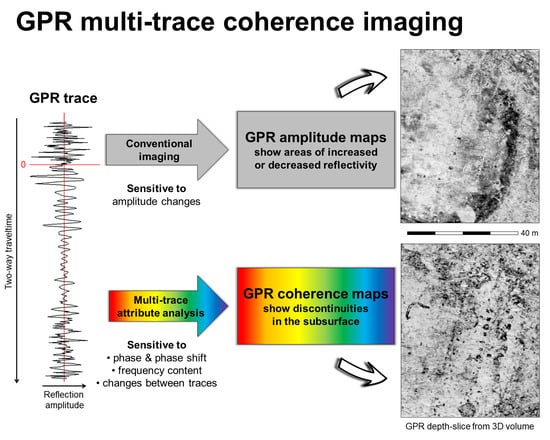
Current state-of-the-art in GPR data visualisation for archaeological prospection surveys is the generation of GPR amplitude maps in the form of GPR time- or depth-slices [5] that sometimes are referred to as C-scans ([6], p. 248). These horizontal data slices are often averaged over a vertical time- or depth-range in order to enhance the visual appearance of structures and anomalies of interest. The generation of such thick slices, in contrast to single-sample slices [7], requires the envelope computation through Hilbert transformation of the GPR traces in order to prevent possible amplitude cancellations when averaging positive and negative amplitude values within a time- or depth-window. This process inevitably reduces the vertical resolution of the GPR data. In order to exploit the full vertical resolution of the data, full-amplitude single-sample GPR depth-slices can be generated, resulting in slices of as little as 6 mm thickness in the case of 400 MHz impulse GPR data. However, the frequent polarity reversal associated with single-sample, full-amplitude slice visualisations, when moving up and down through the data volume and stack of slices, respectively, can obscure the structural information and complicate the understanding of the imaged anomalies.
Three-dimensional GPR data volumes and the contained individual GPR traces comprise beyond simple amplitude values much more information, information that currently is rarely utilised by common GPR data analysis and visualisation techniques. Since GPR data resemble in many respects reflection seismic data [8], it suggests itself to adapt effective algorithms developed for the processing of exploration seismic data to GPR data imaging. In particular, post-stack seismic trace attribute analysis [9] appears to offer promising avenues for the advancement of GPR data visualisation and high-resolution subsurface imaging.
2. Material and Methods
2.1. Seismic Trace Attribute Analysis
In the field of reflection- or exploration-seismology, seismic traces are recorded time series of the acoustic energy that has returned to the surface after reflection from interfaces and discontinuities in the subsurface. Seismic traces comprise many wavelets with different amplitude, frequency and phase shifts. Seismic attributes are quantities that can be extracted or derived from the seismic data to enhance information that may not be obvious in standard amplitude based data visualisations, thus permitting improved possibilities for data analysis and interpretation [9,10,11,12,13,14]. Seismic attributes can be differentiated into several groups. Taner suggested a classification of seismic attributes into physical and geometric attributes [15], with physical relating to wave propagation, lithology, and other physical parameters, and geometrical relating to dip and azimuth of maximum coherency directions. In reflection seismology it is common to differentiate between pre-stack and post-stack seismic attributes. According to Taner, both pre-stack and post-stack attributes classify into the two sub-classes of instantaneous attributes and wavelet attributes. An alternative classification divides between amplitude attributes, time/horizon attributes, and frequency attributes [16]. Amplitude attributes are mean amplitude, average energy, root mean square amplitude, maximum magnitude, amplitude versus offset (AVO) attributes, and the anelastic attenuation factor. Time/horizon attributes are coherence, dip, azimuth, and curvature. Multi-trace seismic attributes are computed from more than one input trace. They are used to determine coherence, dip and azimuth, or curvature. In general, for most GPR data analogies, only seismic post-stack attributes are of interest. Geophysicists Kurt Marfurt from the University of Oklahoma and Satinder Chopra are the authorities when it comes to seismic attribute and coherence analysis and imaging [17]. The study by Kurt Marfurt headed Research Consortium on Attribute-Assisted Seismic Processing & Interpretation (AASPI) has made a rich set of presentations and course notes on seismic attribute analysis available online [18].
The goal of exploration seismology, as much as GPR measurements for archaeological prospection, is the detection and identification of specific anomalous regions and structures in the data, which in general are caused by discontinuities in the subsurface. In the case of reflection seismic surveys, the geological stratification of sedimentary deposits may have been disturbed for instance by erosion channels, intrusions such as salt domes, or fracturing of the rock. The corresponding anomalies can be of great interest for hydrocarbon exploration and reservoir studies. Therefore, the most common attribute used for seismic data analysis, aside from amplitude mapping, is coherence, semblance or discontinuity. According to Chopra [19], coherence is a seismic attribute that measures the similarity between neighbouring seismic traces in 2D or 3D seismic data. It is mainly used to image faults and lateral structural and stratigraphic discontinuities in the data. Coherence mapping is used to enhance stratigraphic information that otherwise may be difficult to extract from the data [20].
On archaeological sites, the subsurface has been disturbed by past human activities, such as the construction of public, private and defensive architecture, including infrastructure installations (e.g., track ways, road pavings, channels, pipes), monuments, fortifications, the excavation of graves, pits, trenches, or the deposition of waste, dirt, bodies, and objects. Any such disturbance could result in discontinuities in the corresponding geophysical prospection data, which thus can be observed as so-called anomalies [21]. This is why the discontinuity, expressed through the coherence or semblance attribute, is of particular interest when it comes to the analysis of GPR data acquired for archaeological prospection. Earlier applications of seismic attribute analysis to the processing of GPR data have been reported by Grasmueck [22], Henryk and Golebiowski [23], Tronicke and Böninger [15,24,25,26,27], Zhao et al. [28,29,30], and Morris et al. [31]. Zhao et al. [29] made use of instantaneous phase, instantaneous amplitude, frequency slope fall and median frequency to image a prehistoric canoe surveyed by GPR. Böninger and Tronicke first convincingly demonstrated the feasibility of attribute-based GPR data processing using amplitude, energy, coherency and similarity to image tombs in relatively small high-resolution GPR data sets, covering areas of 6 × 12 m and 8 × 14 m size [26]. In another publication [25], they describe the use of similarity, energy, analytical signal, topographic slope, and similarity for the analysis of GPR data collected at the palace garden of Paretz in Germany, covering an area of some 30 × 40 m. In a further study [27], symmetry and principal component analysis polarisation attributes are used for the imaging of GPR data acquired across an area of 24 × 32 m. Tronicke and Böninger [15] discuss how attribute analysis can be a valuable technique for the analysis and interpretation of GPR data, illustrating it with a data example covering an area of 20 × 60 m. In this paper, we will focus on the computation and visualisation of the coherence attribute for extensive high-resolution GPR data volumes, and the subsequent data analysis.
2.2. GPR Coherence and Discontinuity Analysis
GPR reflection amplitudes are suited to image and map structures in the subsurface that are strongly reflecting, such as stones, stone layers or remains of stone or brick walls, or that alternatively show increased signal absorption, such as the filling of pits, trenches or postholes. Furthermore, interfaces between layers with different dielectric properties can give rise to increased or decreased reflection amplitudes of the transmitted GPR source pulse. Depending on the electromagnetic properties of the traversed material, frequency dependent absorption and damping of the GPR signal can occur.
Continuity, coherence or semblance (cf. resemblance, similarity) exists in GPR data when adjacent GPR traces are highly equal in regard to amplitude, phase shift and frequency content. As stated above, inhomogeneities in the subsurface can cause discontinuities in the recorded GPR data. Thus, it is possible and sensible to compare neighbouring GPR traces in the 3D data volume in order to image areas and zones of discontinuity, dissimilarity or incoherence. Kington [32,33] presented different methods used to compute semblance, coherence and discontinuity attributes for seismic data analysis. He described first the work of Bahorich and Farmer [34] who used simple cross-correlation between three traces. Kington [33] notes that this method is sensitive to noise, and that Marfurt et al. [35] generalised this approach to an arbitrary number of input traces, referring to it as semblance-based coherence computation. He explains that this new method is computationally faster and less susceptible to noise, but it is sensitive to lateral amplitude changes and phase differences. Therefore, according to Kington, Gersztenkorn and Marfurt [36] proposed an Eigenstructure-based algorithm to remove amplitude sensitivity for the enhanced imaging of subtle structures. In order to differentiate between dipping reflectors and local discontinuities, as such caused by fault zones, Marfurt [37] proposed a structural dip correction that can be applied to the Kington mentioned methods. Kington describes finally the Gradient Structure Tensor (GST) method proposed by Randen et al. [38] as an alternative approach to discontinuity analysis. The GST approach can be used for the automated interpretation of seismic data based on the analysis of texture attributes by analysing “the variability in the local gradient within a moving window” [33]. The method estimates a gradient vector, a local gradient covariance matrix, and uses then a principal component analysis where the principal eigenvector represents the normal to the dip and azimuth of the local reflection.
As a first attempt, we have implemented in the in-house developed GPR processing software ApRadar a simple cross-correlation approach involving adjacent GPR traces for the computation of the coherence [C]. For each sample of each GPR trace, first a correlation [] with another neighbouring trace over a certain time window is computed, normally for one (±0.5) or two (±1.0) wavelengths, with the wavelength defined via the nominal frequency of the GPR antenna used. Then, the coherence is obtained by subtracting the correlation from 1.0:
The correlation is in the range of [−1, …, +1]: it is +1 for two identical time series and −1 in the case of a phase shift of 180. Therefore, the coherence computes to the range of [0, …, +2], with a value of zero meaning no deviation between traces, and +2 in case of a very large deviation.
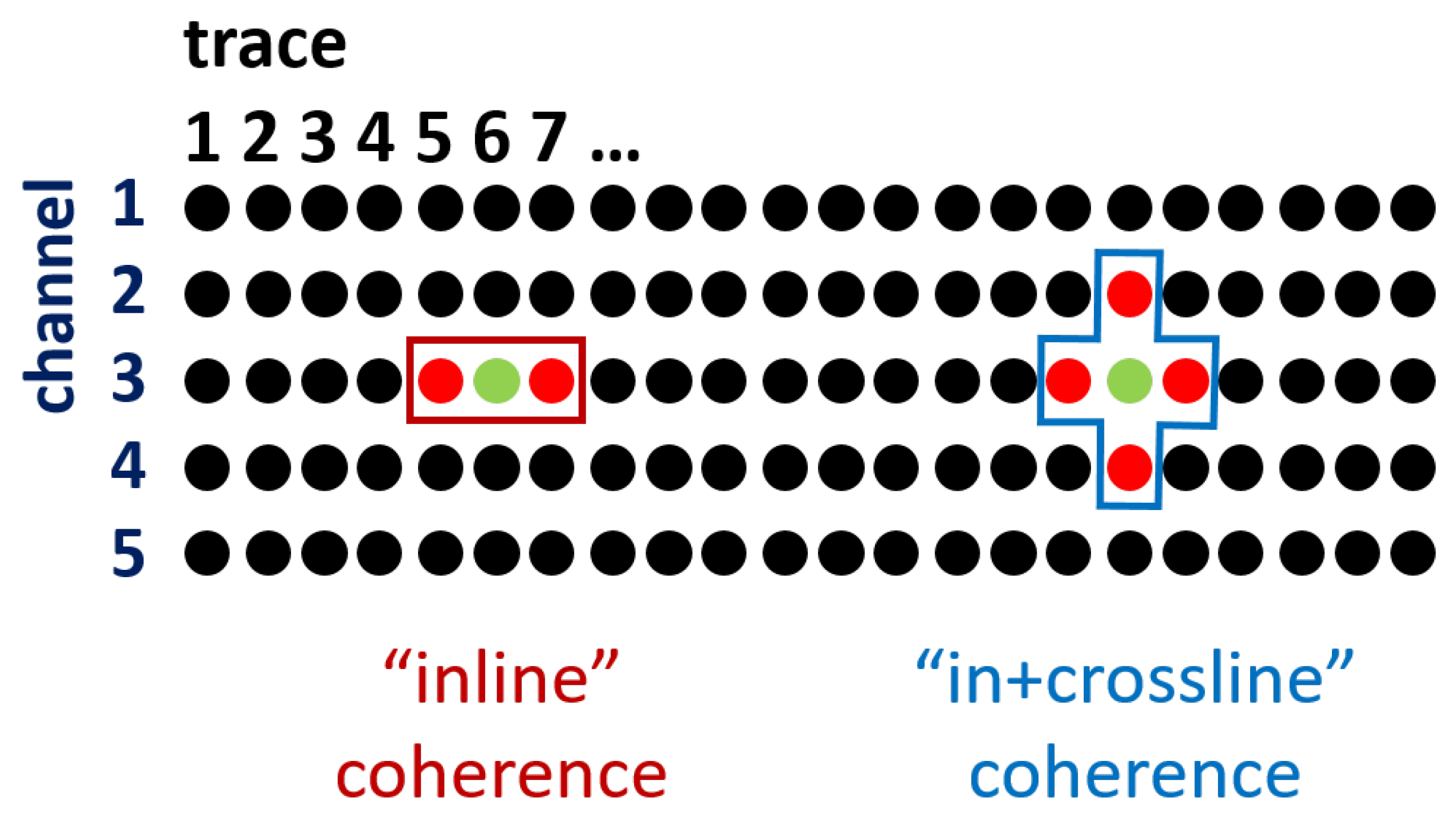
We have implemented two geometrically different ways to compute the coherence with regard to neighbouring GPR traces, termed inline and in+crossline coherence, respectively (Figure 1). In the case of the inline coherence [], three traces are used: the central trace ( ![Remotesensing 12 01583 i001]() ), the one before and the one after (
), the one before and the one after ( ![Remotesensing 12 01583 i002]() ). Thus, two coherences are computed, and , to determine :
). Thus, two coherences are computed, and , to determine :
 ), the one before and the one after (
  ). Thus, two coherences are computed, and , to determine :
The in+crossline coherence [] is computed by using the three traces of the inline coherence as well as the two traces next to the central trace in the neighbouring channels. Thus, in total, five traces are used:
The particular challenges arising for coherence data processing are the necessity for the exact determination of time-zero, and, in the case of inline and in+crossline coherence calculations of data acquired with multi-channel systems, as in the examples shown and discussed below, the consideration of the slightly different signal shapes transmitted/recorded by different adjacent antennae. Time-zero determination is much more critical for coherence calculations than in the case of conventional amplitude slice visualisations because of its effect on phase shifts of the individual traces. If time-zero is not determined precisely for each individual trace, then deviations in coherence will result for all time samples of the trace in question. For each trace, time-zero is calculated individually with sub-pixel accuracy by adjusting a trace averaged from the measurement data by coherence calculation. This elaborate computation is necessary because of the constantly ever so slightly changing coupling of the antennas in the multi-antenna array boxes in the case of real measurements, which cause slightly different waveforms of the first wavelet. The zero crossing of the near-field signal is used, which is the crossing between the maxima and minima, respectively, of the primary and secondary pulse. In the case of the16-channel 400 MHz MALÅ Imaging Radar Array (MIRA) commonly employed by us, the recorded signature is highly stable, permitting accurate determinations of the zero crossing. A precise time-zero determination is particularly important for the calculation of the crossline coherence, which takes adjacent channels recorded with different antennae into account.
The data processing prior to the computation of the coherence is basically the same as for the generation of Hilbert-transformed GPR depth-slices, though of course omits the envelope trace calculation itself. First, a dewow filter is applied to remove the DC component from the GPR traces. Then, the data are bandpass filtered to eliminate frequency content below half the nominal antenna frequency, as well as above twice its value. Although the GPR antennae should in general be shielded to prevent unwanted reflections from structures located above the ground surface, the recorded GPR signal is actually affected by disturbances that do not originate from the subsurface. Spurious reflections can be caused by the antenna construction itself, the mounting frame of the antenna, and in the case of motorised measurement systems, from the towing or pushing vehicle. These disturbances are predominantly constant and thus can be removed through computation and subtraction of an average trace. To this purpose, a moving average trace is calculated for a range of ±10–20 m before and after the central trace. Finally, if desired, a Kirchhoff migration can be performed.
For visualisation, the GPR amplitude values are replaced with the coherence values prior to computation of the depth-slices. Individual channels are adjusted by multiplication in order to adjust for slight differences between the channels, levelling them on the same mean value, before they are projected into the 3D data volume. The data are then exported as GeoTiff images and visualised in such a way that breaklines and changes in the waveform are displayed as black or dark grey values, while coherent areas show as white or light grey values. Thick depth-slices are generated by summing coherence values over a certain depth-range. Migration of the data can focus the images and can reduce linear noise and distortions that mostly occur in the inline direction of the measurements. As in the case of amplitude maps, migration can result in geometrically more realistic images and thereby facilitate data interpretation.
3. Results—Coherence Imaging Examples
Below, three examples for coherence imaging taken from extensive high-resolution GPR data sets illustrate the potential of this approach. Conventional GPR depth-slice images in the form of amplitude maps are presented alongside coherence maps for the same depth-ranges. All examples shown here are from Scandinavian sites where our coherence imaging tests resulted in notable benefits. These single-phase sites and corresponding archaeological remains appear to be more suitable for coherence imaging than common, multi-phase continental sites with buried Medieval or Roman architectural remains that often come along with complex overburden and strongly inhomogeneous strata. The subtle changes associated with the stratification of filled pits, postholes, and trenches encountered on Scandinavian Iron Age sites seem to be appropriate for the imaging of discontinuities expressed in phase and frequency shifts rather than strong amplitude contrasts. The coherence imaging approach is currently tested on a variety of high-resolution GPR data sets from different regions, covering diverse types of archaeological remains. The outcome of this study will be published separately.
3.1. Rysensten—Denmark
In 2014, the LBI ArchPro in collaboration with Holstebro Museum conducted a geophysical archaeological prospection pilot study at archaeological sites in West Jutland, Denmark. Among others, the site of an abandoned medieval village near Rysensten was surveyed [4,39]. The medieval village of Rysensten is thought to have existed between AD 1050 and AD 1536, and its remains are situated in sandy soil. The site, located close to the coast of the North Sea and the manor of Rysensten on a plateau between the River Ramme and Nissum Fjord, had been discovered by aerial photography [40]. The crop-marks showed rows of postholes, pits and boundary trenches belonging to more than 15 long houses. Here, in total 11.6 ha of the area was surveyed with a motorised 16-channel 400 MHz MIRA system with 8 cm crossline channel spacing and 4 cm inline trace spacing. The data have been processed to form a 3D data volume with 8 × 8 cm horizontal voxel size.
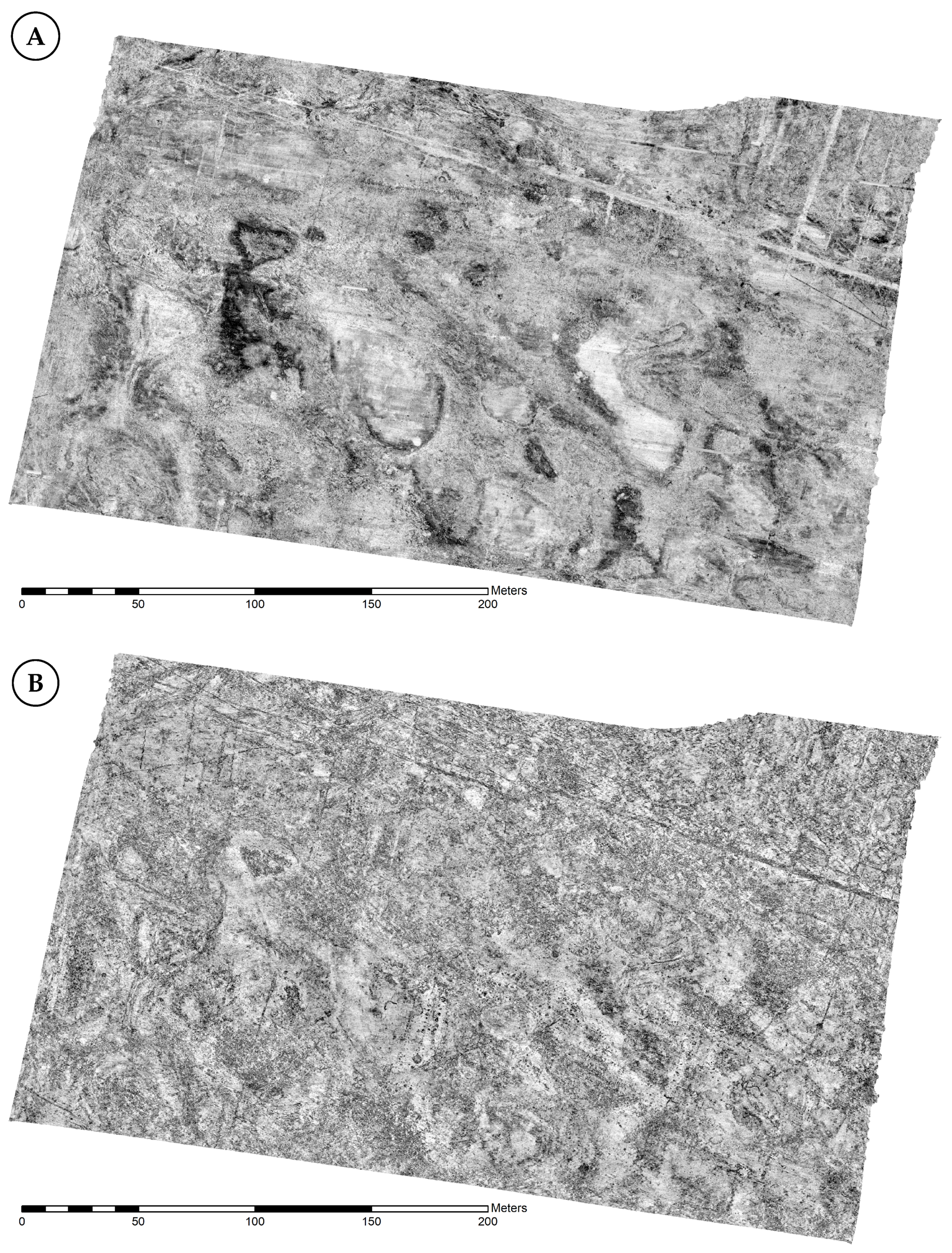
In general, the GPR amplitude maps from Rysensten are dominated by broad, long-wavelength, reflective and absorbing bands associated with geological interfaces between different soil layers (Figure 2A and Figure 3A). The geometry of these sandy soil layers appears to be caused by dune like structures. Aside from these extensive anomalies originating from geological inhomogeneities in the subsurface, broad linear absorbing anomalies associated with human-made drainage trenches, some of which running parallel or perpendicular to each other, dominate the amplitude maps. The archaeological remains, which predominantly appear to be filled pits, postholes or trenches, have been dug into these soil layers. In the conventional GPR amplitude depth-slices it is possible to see these features, as expected, as absorbing anomalies in areas of increased reflectivity, down to 1–1.2 m depth.
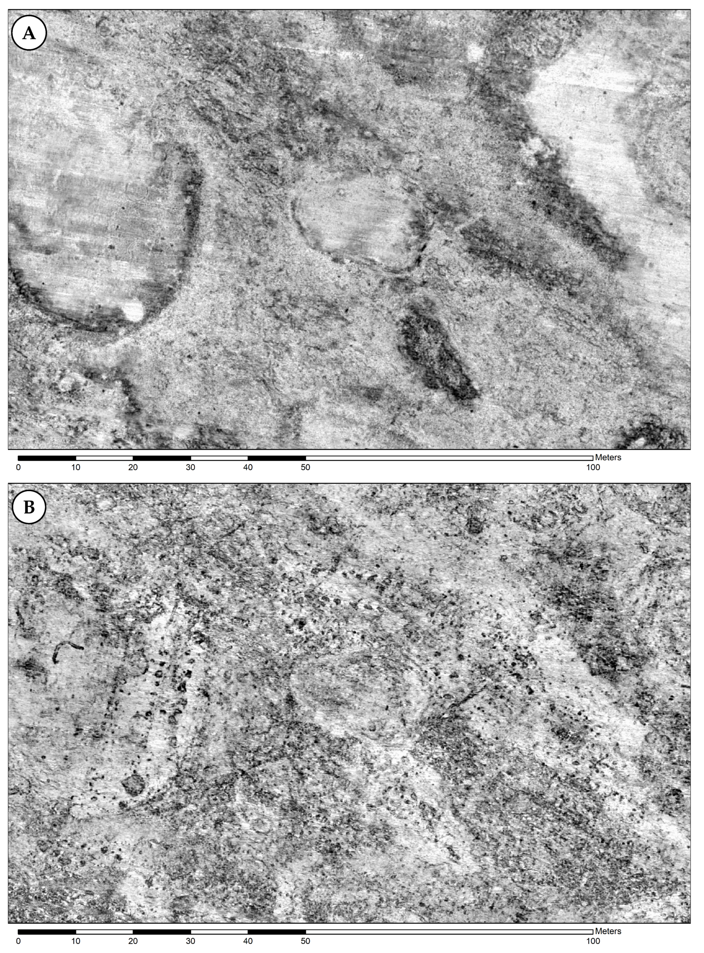
The corresponding coherence maps show the large banded anomalies caused by the natural soil stratification hardly at all (Figure 2B and Figure 3B). Instead, these alternative data visualisations highlight anomalies associated with short-wavelength structures and abrupt discontinuities in the subsurface, irrespective of the reflection amplitudes caused by these structures. The level of detail contained in the coherence maps can be best appreciated when zooming into the data images (Figure 3). Small-scale anomalies that are barely visible in the amplitude maps and that are caused by distinct discontinuities across short distances, associated with pits, postholes and small trenches that have been dug or cut into the natural soil layering, stand out in the coherence slices, in which lowest coherence is indicated with black colour. The geometrical arrangement of the coherence anomalies visible in the data from Rysensten, forming rows of anomalies presumably associated with remains of postholes or pits, some of which are aligned in parallel, indicates the presence of several building remains. The coherence maps show the archaeological remains in greater quantity and clarity compared to the amplitude maps.
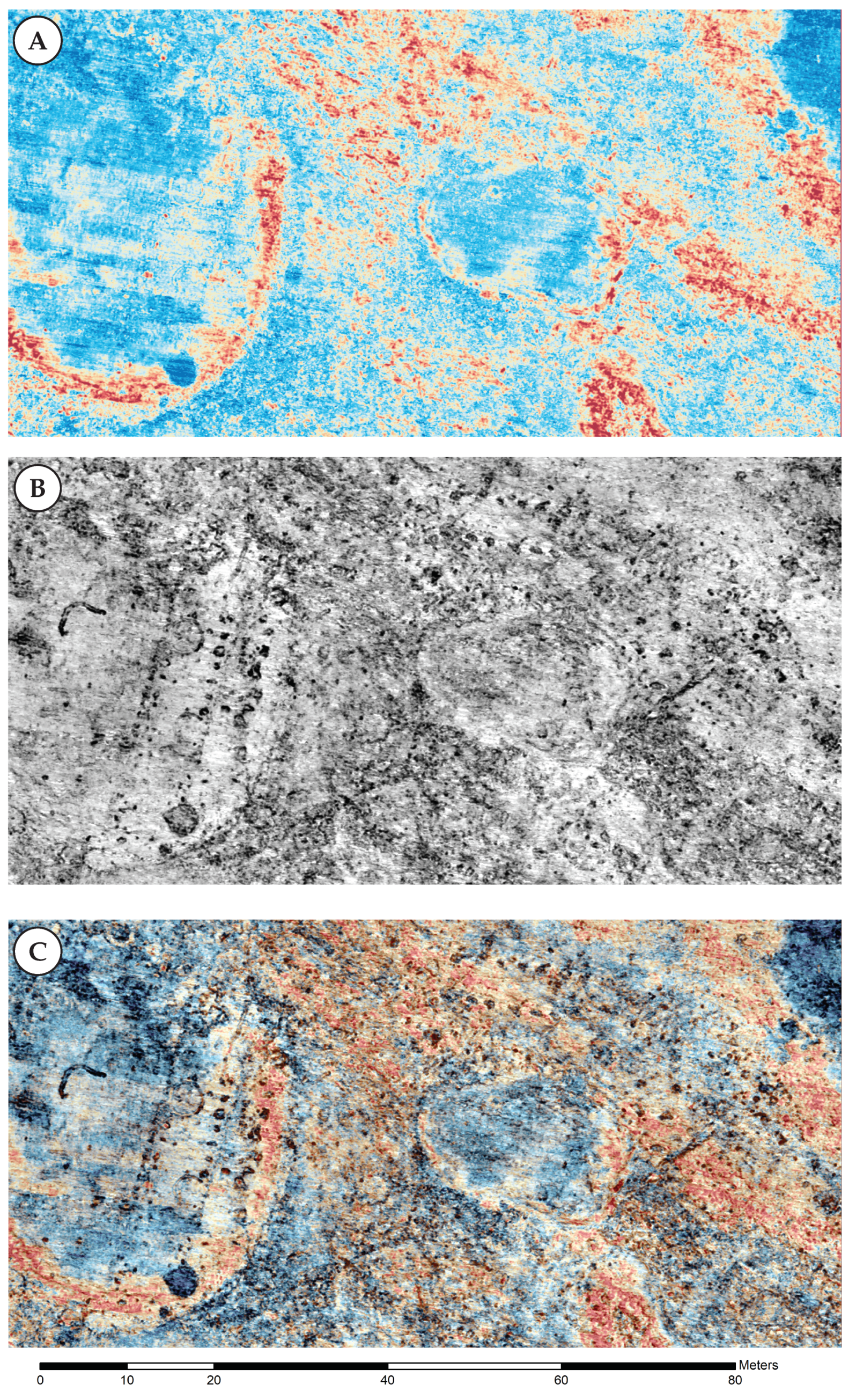
A possibility to jointly utilise and analyse both amplitude and coherence maps is the combination of corresponding data visualisations through image fusion [41,42]. For this purpose, the different data are visualised using different colour representations: one data set is mapped to 254 grey-scale values while the other is visualised using a symmetrical seismic colour-map, blending linearly from dark red via red to white to blue and then dark blue. Figure 4 illustrates this approach, in which the grey-scale amplitude data has been mapped to a seismic colour scale (Figure 4A), while the coherence data has been visualised using a grey-scale representation (Figure 4B). The fused image (Figure 4C) combines the information contained in both data visualisations, facilitating the understanding of the subsurface situation. In this case, a simple normal blending method with an alpha value of 0.425 for the top image (A) with subsequent contrast normalisation has been used.
3.2. Stadil Mølleby—Denmark
The same MIRA system as the one used at Rysensten was deployed in September 2014 to survey the Viking Age settlement site of Stadil Mølleby in Denmark, which likewise had been discovered by aerial archaeology ([40], p. 137). In general, the results obtained here were very similar to those of Rysensten, consisting of building remains in the form of pits, postholes and trenches dug into sandy soil layers [4,39]. The settlement comprises a considerable number of longhouses, visible in the GPR data as parallel rows of postholes. The amplitude maps are dominated by larger patches of reflecting and absorbing soil (Figure 5A), transected by drainage trenches. The data appear affected by broad, northeast–southwest running surface disturbances, which seem to have been caused by measurement artefacts. Among the extensive, strongly reflecting and absorbing areas, it is difficult to identify the archaeologically relevant structures, mainly pits and postholes that show as small, light coloured, absorbing anomalies. Particular in areas with generally absorbing character, these anomalies become invisible or very difficult to discern.
In the coherence image (Figure 5B), the pattern of the extensive, gradually varying reflectivity of the subsurface does not show, and instead, the incoherencies or discontinuities in the GPR response caused by local soil disturbances become clearly visible. In the case of larger pits and trenches, the edge of the buried structure shows as sharply defined outline. Numerous pit-alignments indicate building remains. The larger hall buildings show as double rows of postholes (Figure 6B). In Figure 7, a fusion of the data shown in Figure 6A,B is shown. Again, a simple normal fusion with an alpha value of 0.4 for the top image (A) has been chosen, with subsequent histogram stretching applied. This approach is suited to integrate the complementary amplitude and coherence data sets for joint interpretation. It has to be kept in mind that in the case of amplitude imaging, coherence imaging, or the interpretation of fused images, the entire stack of generated slices is analysed, which permits of course for a better recognition and understanding of the anomalies and underlying structures. However, in particular, this example shows the great benefit of amplitude-independent coherence or discontinuity imaging for enhanced data analysis and interpretation possibilities.
3.3. Gjellestad Viking Ship Burial
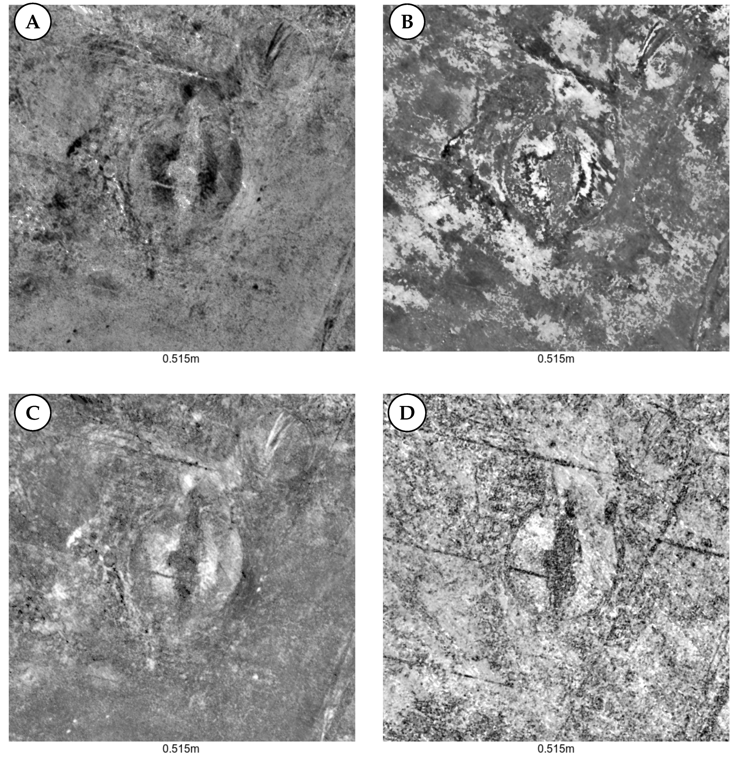
In November 2018, the Norwegian Institute for Cultural Heritage Research (NIKU) and Østfold County—now Viken County—announced the discovery of the assumed remains of a Viking ship made by archaeological GPR prospection in an overploughed burial mound at the site of Gjellestad in Østfold County in Norway [43,44]. Using a motorised 16-channel 400 MHz MIRA system with 10.5 cm crossline trace spacing, a large area next to the monumental Jelle burial mound was investigated. Traces of eight earlier unknown burial mounds destroyed by ploughing where discovered. In one of the former mounds the buried remains of a Viking ship could clearly be identified. There have been indications that the ship’s keel and bottom-most planks are likely to have been preserved in the soil. The Viking ship remains are located immediately below the topsoil at a depth of approximately 50 cm. Archaeological excavations conducted by the University Museum Oslo across the ship structure in summer 2019 have fully confirmed the findings of the GPR survey and the data interpretation of the ship shaped anomaly, as being caused by the remains of a buried Viking ship.
Standard GPR amplitude maps generated after Hilbert transformation of the GPR traces show the remains of a large, north–south oriented, well-defined, circa 20 m long ship-shaped structure as absorbing the anomaly in the circular mound (Figure 8A). By inverting the grey-scale map, the absorbing structures appear dark (Figure 8C). Single-sample amplitude slices show reflective structures with a very high vertical imaging resolution. The appearance of the single-sample slices is fundamentally different to the Hilbert transformed slices, due to the alternating positive and negative amplitude values along each GPR trace (Figure 8B). The coherence images present structures in the subsurface irrespective of the reflected energy, but relative to the amount of discontinuity caused to the recorded time-series within the cross-correlation window. Thus, in this case the edge of the circular mound, the outline of the ship and internal features, the drainage trenches as well as a large number of detailed ground disturbances that do not show in the amplitude maps are visible (Figure 8D). The coherence image is highly detailed and complements the conventional data visualisation. A comparison of the archaeological interpretations based on different data visualisations is not part of this paper. However, from the examples shown, it becomes obvious that coherence imaging is a valuable possibility to reveal structural details that would be missed when using only conventional GPR data imaging.
4. Discussion
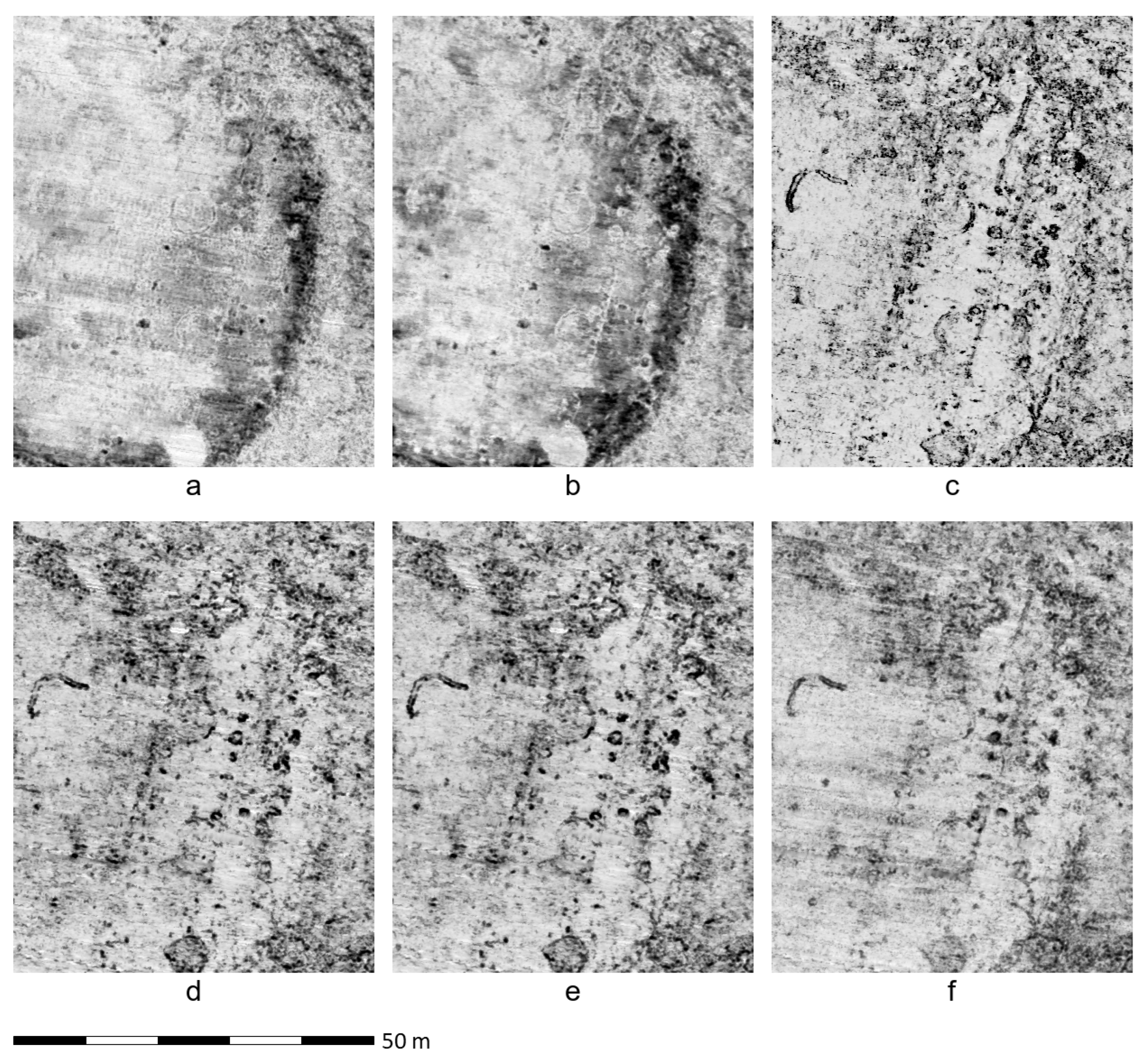
In most of our trials, the in+crossline coherence (Figure 9e) worked better than only inline (Figure 9c) or only crossline (see Figure 9d) coherence, since thus incoherencies in all directions become visible. The inline coherence computation mainly highlights incoherencies in the direction of measurement progress. In the case of more sparsely sampled data, for instance data collected with 25 cm crossline spacing, the results of the inline coherence appear sharper than those of the in+crossline coherence due to the under-sampling in crossline direction.
Migrated coherence images are better defined and focused than non-migrated images. They appear as well richer in contrast, better bringing out the structures. While anomalies associated with pits appear in the unmigrated coherence images as filled structures (Figure 9f), they show as outlining edges in the migrated coherence data (Figure 9e).
According to the online knowledge base [45] of the Society of Exploration Geophysicists on Coherence, the “analysis window chosen can have a significant effect of [sic] the results. Longer windows tend to mix stratigraphy, which can complicate the geologic image”. Kurt Marfurt ([46], slide 54), stated that “Large vertical analysis windows can improve the resolution of vertical faults, but smears dipping faults and mixes stratigraphic features”.
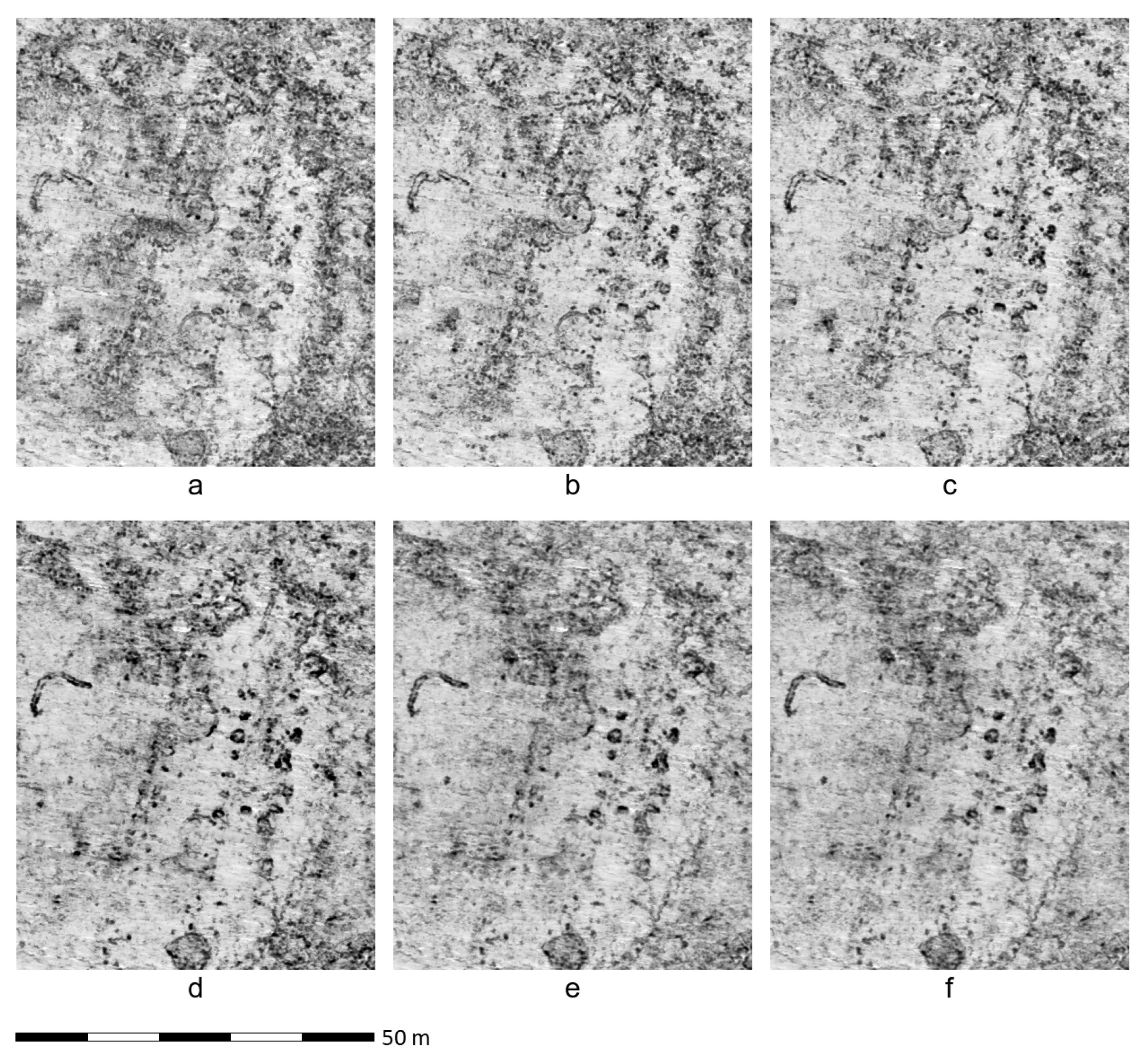
We have made tests regarding the analysis window defined by wavelength and the number of traces involved in the computation of the GPR trace coherence (Figure 10). The wavelength over which the correlation is computed, sensibly should be between one and two wavelengths of the mean transmitted pulse (Figure 10c,d). The wavelength of a 400 MHz pulse is 25 cm. Using less than one wavelength causes an increase in noise (Figure 10a,b). Using more than two wavelengths leads to decreased contrasts and reduced focusing (Figure 10e,f). One to two wave trains correspond to approximately the wavelength of the GPR pulse transmitted by the GPR antenna as well. In the simple approach presented here for coherence imaging based on trace cross-correlations, it is not really meaningful to compute single-sample coherence maps since the coherence computation requires a certain length. Using more than the four directly neighbouring traces does not result in improved images, but increases computation time and decreases the image contrast with increasing number of traces involved.
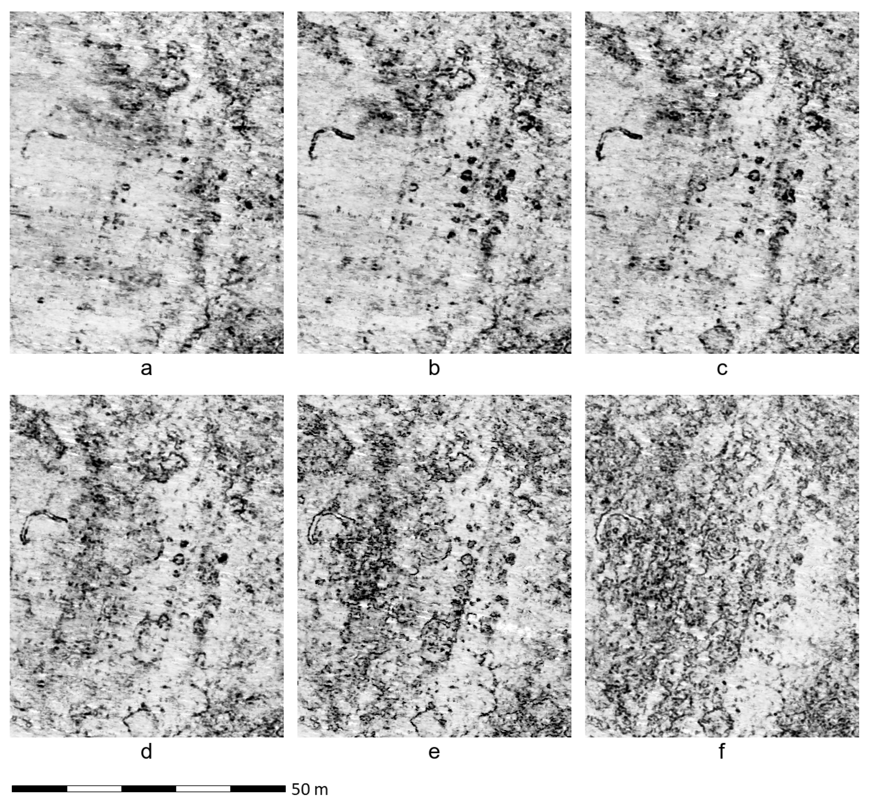
The application of an average-trace removal filter is commonly used for the enhanced imaging of amplitude data. Average-trace removal applied to coherence data can have a strong effect on the resulting depth-slice images. Depending on the distance along which the average-trace is determined, strikingly different outcomes can be achieved (Figure 11). It is thought that the removal of the average-trace in coherence data corresponds a spatial high-pass, or dewow filter that accentuates short-wavelength incoherencies. The larger the effect, the shorter the distance for which the average trace is computed. In the case of our test data, a length of 10 to 20 m for the computation of the average-trace resulted in the clearest structural imaging of small discontinuities in the ground (Figure 11d,e).
Under suitable soil conditions and regarding present archaeological remains, coherence imaging of GPR data appears to be a powerful complement to conventional amplitude mapping. Our tests have shown that in particular Scandinavian Iron Age sites, the prevalent ground conditions can be well suited for this approach. Attempts to use coherence mapping for the imaging of GPR data acquired at Roman sites have so far not been similarly successful. We assume that gains made by coherence imaging are smaller here since the amplitude maps already clearly show to a large extent the anomalies caused by the buried remains of mainly stone built architecture. Further testing is necessary to better evaluate the potential of coherence mapping for other sites and geological backgrounds. Our understanding is that single phase, or not too complex archaeological sites embedded in geologically rather homogeneously stratified soils should be well suited. Kurt Marfurt ([46], slide 54), has summarised coherence imaging for seismic processing and interpretation, which is completely transferable to GPR data visualisation. He states that “coherence
- is an excellent tool for delineating geological boundaries (faults, lateral stratigraphic contacts, etc.),
- allows accelerated evaluation of large data sets,
- provides quantitative estimate of fault/fracture presence,
- often enhances stratigraphic information that is otherwise difficult to extract,
- algorithms are local—faults that have drag, are poorly migrated, or separate two similar reflectors, or otherwise do not appear locally to be discontinuous, will not show up on coherence volumes”.
We can only confirm the observations made by Marfurt [46], slide 25, who noted that the parameters affecting the quality of the coherency imaging results are static corrections and time zero, velocities, data processing filters, and the migration algorithm used. Furthermore, the method used to compute the coherence can considerably enhance the result.
5. Conclusions and Outlook
We have shown that poststack seismic geometrical attribute analysis, specifically coherence analysis, can successfully be applied for the efficient generation of novel useful visualisations of extensive high-resolution GPR data sets collected for archaeological prospection purposes. The here presented and tested coherence algorithm, based on simple trace cross-correlation, is rather primitive compared to the more advanced approaches developed by Gersztenkorn and Marfurt [36], Randen et al. [38] and Marfurt [37]. Thus, there exists still considerable room for methodological improvements of the method with regard to its application to GPR data imaging. Nevertheless, the presented examples show that coherence attribute mapping has the potential to considerably enhance GPR data visualisations and therefore offers new avenues for improved data interpretation, provided that ultra-dense GPR data covering large areas is available, since coarsely sampled data undermines the potential of this method. GPR trace coherence images should be generated routinely alongside conventional amplitude maps to permit for enhanced data interpretations. Aside from geometrical attributes, there exists a number of other seismic attributes of interest when it comes to the development of new promising approaches to GPR data analysis and interpretation. The theoretical groundwork has been laid by seismic processing wizards Satinder Chopra and Kurt Marfurt, among others. It is up to us to pick these low hanging fruits.
Author Contributions
Conceptualization, I.T.; methodology, I.T. and A.H.; software, A.H.; validation, A.H. and I.T.; formal analysis, A.H. and I.T.; investigation, I.T. and A.H.; writing—original draft preparation, I.T.; writing—review and editing, I.T. and A.H.; visualization, A.H. All authors have read and agreed to the published version of the manuscript.
Funding
This research was funded by the Ludwig Boltzmann Institute for Archaeological Prospection and Virtual Archaeology (LBI ArchPro). The LBI ArchPro (archpro.lbg.ac.at) is based on an international cooperation of the Ludwig Boltzmann Gesellschaft (A), Amt der Niederösterreichischen Landesregierung (A), University of Vienna (A), TU Wien (A), ZAMG—Central Institute for Meteorology and Geodynamics (A), Airborne Technologies (A), 7reasons (A), RGZM Mainz—Römisch-Germanisches Zentralmuseum Mainz (D), LWL—Federal state archaeology of Westphalia-Lippe (D), NIKU—Norwegian Institute for Cultural Heritage Research (N), Vestfold fylkeskommune–Kulturarv (N), and ArcTron3D GmbH (D). The research projects at Rysensten and Stadil Mølleby were co-funded by Holstebro Museum (Dk).
Acknowledgments
The fieldwork at Rysensten and Stadil Mølleby was conducted by Roland Filzwieser, Manuel Gabler, Erich Nau and Petra Schneidhofer. The authors thank Lis Helles Olesen for kind permission to publish the data examples from Denmark. The Gjellestad data was collected by Erich Nau and Lars Gustavsen from the Norwegian Institute for Cultural Heritage Research (NIKU) in a survey conducted by NIKU on behalf of Østfold County, now Viken County. The authors thank Sigrid Mannsåker Gundersen and Viken County Council as well as Knut Paasche from NIKU for kind permission to publish the Gjellestad data. Roland Filzwieser has kindly proofread the manuscript. Three anonymous reviewers helped to improve the manuscript.
Conflicts of Interest
The authors declare no conflict of interest.
Abbreviations
The following abbreviations are used in this manuscript:
| AT | Average-Trace |
| LBI ArchPro | Ludwig Boltzmann Institute for Archaeological Prospection and Virtual Archaeology |
| GPR | Ground-Penetrating Radar |
| GST | Gradient Structure Tensor |
References
- Conyers, L. Ground-Penetrating Radar for Archaeology, 3rd ed.; Rowman and Littlefield Publishers, Alta Mira Press: Lanham, MD, USA, 2013. [Google Scholar]
- Leckebusch, J. Ground-penetrating Radar: A Modern Three-dimensional Prospection Method. Archaeol. Prospect. 2003, 10, 213–240. [Google Scholar] [CrossRef]
- Trinks, I.; Hinterleitner, A.; Neubauer, W.; Nau, E.; Löcker, K.; Wallner, M.; Gabler, M.; Filzwieser, R.; Wilding, J.; Schiel, H.; et al. Large-area high-resolution ground-penetrating radar measurements for archaeological prospection. Archaeol. Prospect. 2018, 25, 171–195. [Google Scholar] [CrossRef]
- Filzwieser, R.; Olesen, L.H.; Neubauer, W.; Trinks, I.; Schlosser Mauritsen, E.; Schneidhofer, P.; Nau, E.; Gabler, M. Large-scale geophysical archaeological prospection pilot study at Viking Age and medieval sites in west Jutland, Denmark. Archaeol. Prospect. 2017, 24, 373–393. [Google Scholar] [CrossRef]
- Goodman, D.; Nishimura, Y.; Rodgers, J.D. GPR Time Slices in Archaeological Prospection. Archaeol. Prospect. 1995, 2, 85–89. [Google Scholar]
- Daniels, D.J. Ground penetrating radar. In Encyclopedia of RF and Microwave Engineering; Chang, K., Ed.; Wiley-Interscience: Hoboken, NJ, USA, 2005. [Google Scholar]
- Trinks, I.; Johansson, B.; Gustafsson, J.; Emilsson, J.; Friborg, J.; Gustafsson, C.; Nissen, J.; Hinterleitner, A. Efficient, large-scale archaeological prospection using a true three-dimensional ground-penetrating radar array system. Archaeol. Prospect. 2010, 17, 175–186. [Google Scholar] [CrossRef]
- Fisher, S.C.; Stewart, R.R.; Jol, H.M. Ground Penetrating Radar (GPR) Data Enhancement Using Seismic Techniques. J. Environ. Eng. Geophys. 1996, 1, 89–157. [Google Scholar] [CrossRef]
- Chopra, S.; Marfurt, K.J. Seismic attributes—A historical perspective. Geophysics 2005, 70, 3SO–28SO. [Google Scholar] [CrossRef]
- Chopra, S.; Marfurt, K.J. Seismic attributes—A promising aid for geological prediction. CSEG Recorder 2006, 31, 115–126. [Google Scholar]
- Randen, T.; Sønneland, L. Atlas of 3D Seismic Attributes. In Mathematical Methods and Modelling in Hydrocarbon Exploration and Production. Mathematics in Industry; Iske, A., Randen, T., Eds.; Springer: Berlin/Heidelberg, Germany, 2005. [Google Scholar]
- Sheriff, R.E. Encyclopedic Dictionary of Applied Geophysics, 4th ed.; Society of Exploration Geophysicists: Houston, TX, USA, 2002. [Google Scholar]
- Eastwood, J. Introduction—The attribute explosion. Lead. Edge 2002, 21, 994–995. [Google Scholar] [CrossRef]
- Taner, M.T.; Koehler, F.; Sheriff, R.E. Complex seismic trace analysis. Geophysics 1979, 44, 1041–1063. [Google Scholar] [CrossRef]
- Tronicke, J.; Böninger, J. GPR attribute analysis: There is more than amplitudes. First Break 2013, 31, 103–108. [Google Scholar]
- Wikipedia Contributors. Seismic Attribute—Wikipedia, The Free Encyclopedia. 2018. Available online: https://en.wikipedia.org/wiki/Seismic_attribute (accessed on 15 May 2020).
- Chopra, S.; Marfurt, K.J. Seismic Attributes for Prospect ID and Reservoir Characterization; SEG/EAGE, 2007. Available online: https://library.seg.org/doi/abs/10.1190/1.9781560801900 (accessed on 15 May 2020).
- Marfurt, K.J. Attribute-Assisted Seismic Processing & Interpretation. Available online: http://mcee.ou.edu/aaspi/index.html (accessed on 15 May 2020).
- Chopra, S. Adding the coherence dimension to 3D seismic data. CSEG Rec. 2001, 26, 5–8. [Google Scholar]
- Nissen, S.; Interpretive Aspects of Seismic Coherence and Related Multi-trace Attributes; Reservoir Characteristics of Morrow/Incised-Valley Fill Plays Workshop & Morrow Incised-Valley Core Workshop. Kansas Geological Surveys, Wichita, Kansas, February 2000. Available online: http://www.kgs.ku.edu/Workshops/IVF2000/nissan-ivf/tocnav1.html (accessed on 15 May 2020).
- Lyatsky, H. The Meaning of Anomaly. Explor. Geophys. 2004, 29, 50–51. [Google Scholar]
- Grasmueck, M. 3-D ground-penetrating radar applied to fracture imaging in gneiss. Geophysics 1996, 61, 1050–1064. [Google Scholar] [CrossRef]
- Henryk, M.; Golebiowski, T. Analysis of GPR Trace Attributes and Spectra for LNAPL Contaminated Ground. In Proceedings of the Near Surface 2006—12th EAGE European Meeting of Environmental and Engineering Geophysics, Helsinki, Finland, 4–6 September 2006. [Google Scholar]
- Böninger, U. Attributes and their potential to analyze and interpret 3D GPR data. Ph.D. Thesis, Potsdam University, Potsdam, Germany, 2010. [Google Scholar]
- Böninger, U.; Tronicke, J. Integrated data analysis at an archaeological site: A case study using 3D GPR, magnetic, and high-resolution topographic data. Geophysics 2010, 75, B169–B176. [Google Scholar] [CrossRef]
- Böninger, U.; Tronicke, J. Improving the interpretability of 3D GPR data using target-specific attributes: Application to tomb-detection. J. Archaeol. Sci. 2010, 37, 360–367. [Google Scholar] [CrossRef]
- Böninger, U.; Tronicke, J. Subsurface Utility Extraction and Characterization: Combining GPR Symmetry and Polarization Attributes. IEEE Trans. Geosci. Remote. Sens. 2012, 50, 736–746. [Google Scholar] [CrossRef]
- Zhao, W.; Forte, E.; Pipan, M.; Tian, G. Ground Penetrating Radar (GPR) attribute analysis for archaeological prospection. J. Appl. Geophys. 2013, 97, 107–117. [Google Scholar] [CrossRef]
- Zhao, W.; Tian, G.; Wang, B.; Forte, E.; Pipan, M.; Lin, J.; Shi, Z.; Li, X. 2D and 3D imaging of a buried prehistoric canoe using GPR attributes: A case study. Near Surf. Geophys. 2013, 11, 457–464. [Google Scholar] [CrossRef]
- Zhao, W.; Forte, E.; Pipan, M. Texture Attribute Analysis of GPR Data for Archaeological Prospection. Pure Appl. Geophys. 2016, 173, 2737–2751. [Google Scholar] [CrossRef]
- Morris, I.; Abdel-Jaber, H.; Glisic, B. Quantitative Attribute Analyses with Ground Penetrating Radar for Infrastructure Assessments and Structural Health Monitoring. Sensors 2019, 19, 1637. [Google Scholar] [CrossRef] [PubMed] [Green Version]
- Kington, J. Semblance, coherence, and other discontinuity attributes. Lead. Edge 2015, 34, 1426–1544. [Google Scholar] [CrossRef]
- Kington, J. Semblance, Coherence, and other Discontinuity Attributes. Available online: https://github.com/seg/tutorials-2015/blob/master/1512_Semblance_coherence_and_discontinuity/Discontinuity_tutorial.ipynb (accessed on 15 May 2020).
- Bahorich, M.; Farmer, S. 3-D seismic discontinuity for faults and stratigraphic features: The coherence cube. Lead. Edge 1995, 14, 1053–1058. [Google Scholar] [CrossRef]
- Marfurt, K.; Kirlin, R.L.; Farmer, S.L.; Bahorich, M.S. 3-D seismic attributes using a semblance-based coherency algorithm. Geophysics 1998, 63, 1150–1165. [Google Scholar] [CrossRef] [Green Version]
- Gersztenkorn, A.; Marfurt, K.J. Eigenstructure-based coherence computations as an aid to 3-D structural and stratigraphic mapping. Geophysics 1999, 64, 1468–1479. [Google Scholar] [CrossRef]
- Marfurt, K.J. Robust estimates of 3D reflector dip and azimuth. Geophysics 2006, 71, 29–40. [Google Scholar] [CrossRef]
- Randen, T.; Monsen, E.; Signer, C.; Abrahamsen, A.; Hansen, J.O.; Sæter, T.; Schlaf, J. Three-dimensional texture attributes for seismic data analysis. In Proceedings of the 70th Annual International Meeting; Expanded Abstracts; SEG: Tulsa, OK, USA, 2000; pp. 668–671. [Google Scholar]
- Filzwieser, R.; Neubauer, W.; Trinks, I.; Olesen, L.; Verhoeven, G.; Mauritsen, E.; Schneidhofer, P.; Nau, E.; Gabler, M. Geofysiske undersøgelser og luftfotoarkæologi i Vestjylland. In Luftfotoarkæologi 2; Olesen, L., Mauritsen, E., Broch, M., Eds.; De Kulturhistoriske Museer i Holstebro Kommune: Copenhagen, Denmark, 2019; pp. 163–177. [Google Scholar]
- Olesen, L.; Mauritsen, E. Luftfotoarkæologi i Danmark; Holstebro Museum: Holstebro, Denmark, 2015; pp. 140–142. [Google Scholar]
- Verhoeven, G.; Nowak, M.; Rebecca, N. Pixel-level image fusion for archaeological interpretative mapping. In Proceedings of the 8th International Congress on Archaeology, Computer Graphics, Cultural Heritage and Innovation ‘ARQUEOLÓGICA 2.0’, Valencia, Spain, 5–7 September 2016; pp. 404–407. [Google Scholar]
- Filzwieser, R.; Olesen, L.; Verhoeven, G.; Mauritsen, E.; Neubauer, W.; Trinks, I.; Nowak, M.; Nowak, R.; Schneidhofer, P.; Nau, E.; et al. Integration of Complementary Archaeological Prospection Data from a Late Iron Age Settlement at Vesterager—Denmark. J. Archaeol. Method Theory 2018, 25, 313–333. [Google Scholar] [CrossRef]
- NIKU. The Gjellestad Ship. Available online: https://www.niku.no/en/prosjekter/jellestadskipet/ (accessed on 15 May 2020).
- Gustavsen, L.; Gjesvold, P.; Gundersen, S.; Hinterleitner, A.; Nau, E.; Paasche, K. Gjellestad—A newly discovered central place in South-East Norway. Antiquity 2020, in press. [Google Scholar]
- SEG Wiki. Coherence. Available online: https://wiki.seg.org/wiki/Coherence (accessed on 15 May 2020).
- Marfurt, K. 3D Seismic Attributes for Prospect Identification and Reservoir Characterization—Introduction; AASPI, University of Oklahoma: Norman, OK, USA, 2016. [Google Scholar]
Figure 1.
Top-view of the ground-penetrating radar (GPR) traces used for inline and in+crossline coherence computation.
Figure 1.
Top-view of the ground-penetrating radar (GPR) traces used for inline and in+crossline coherence computation.

Figure 2.
7.4 ha area GPR survey at Rysensten. (A) Conventional GPR amplitude map after Hilbert transformation of the data showing a 5 cm thick depth-slice from approximately 40–45 cm depth. (B) Coherence map for the same depth range. North is pointing upwards for all data figures in this article.
Figure 2.
7.4 ha area GPR survey at Rysensten. (A) Conventional GPR amplitude map after Hilbert transformation of the data showing a 5 cm thick depth-slice from approximately 40–45 cm depth. (B) Coherence map for the same depth range. North is pointing upwards for all data figures in this article.

Figure 3.
Detail of the same area of the Rysensten GPR data set. (A) Conventional GPR amplitude map after Hilbert transformation of the data showing a 5 cm thick depth-slice from approximately 40–45 cm depth. (B) Coherence map for the same depth range.
Figure 3.
Detail of the same area of the Rysensten GPR data set. (A) Conventional GPR amplitude map after Hilbert transformation of the data showing a 5 cm thick depth-slice from approximately 40–45 cm depth. (B) Coherence map for the same depth range.

Figure 4.
(A) Conventional GPR amplitude map after Hilbert transformation of the data showing a 5 cm thick depth-slice from approximately 40–45 cm depth using a red-white-blue seismic colour scale. (B) Coherence map for the same depth-range as grey-scale image. (C) Fusion of the two images above.
Figure 4.
(A) Conventional GPR amplitude map after Hilbert transformation of the data showing a 5 cm thick depth-slice from approximately 40–45 cm depth using a red-white-blue seismic colour scale. (B) Coherence map for the same depth-range as grey-scale image. (C) Fusion of the two images above.

Figure 5.
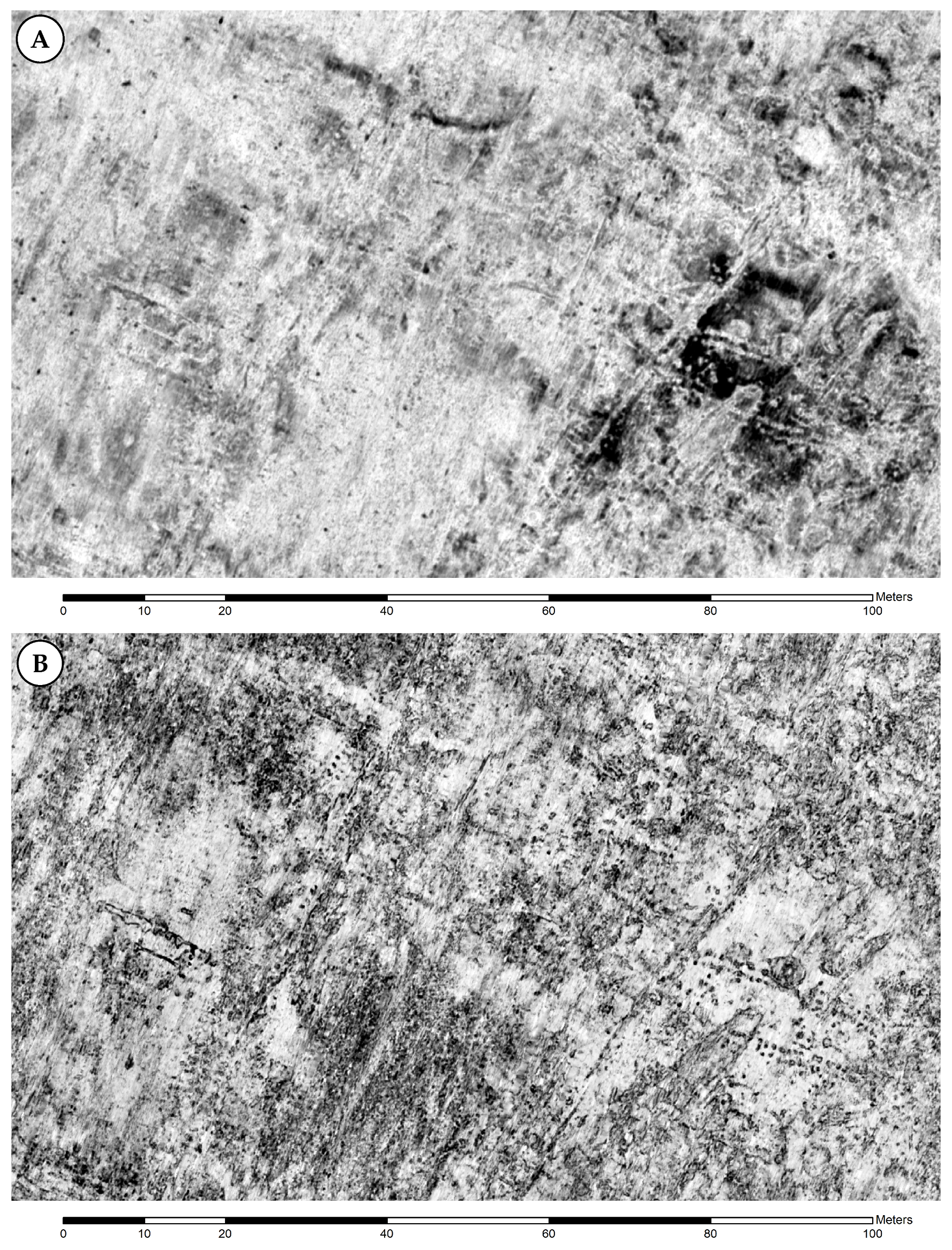
Stadil Mølleby: Migrated GPR depth-slices from 55–85 cm depth showing the same area. (A) Conventional reflection amplitude map. (B) Inline coherence image. Note the numerous rows of pits indicating building remains clearly visible in the coherence image.
Figure 5.
Stadil Mølleby: Migrated GPR depth-slices from 55–85 cm depth showing the same area. (A) Conventional reflection amplitude map. (B) Inline coherence image. Note the numerous rows of pits indicating building remains clearly visible in the coherence image.

Figure 6.
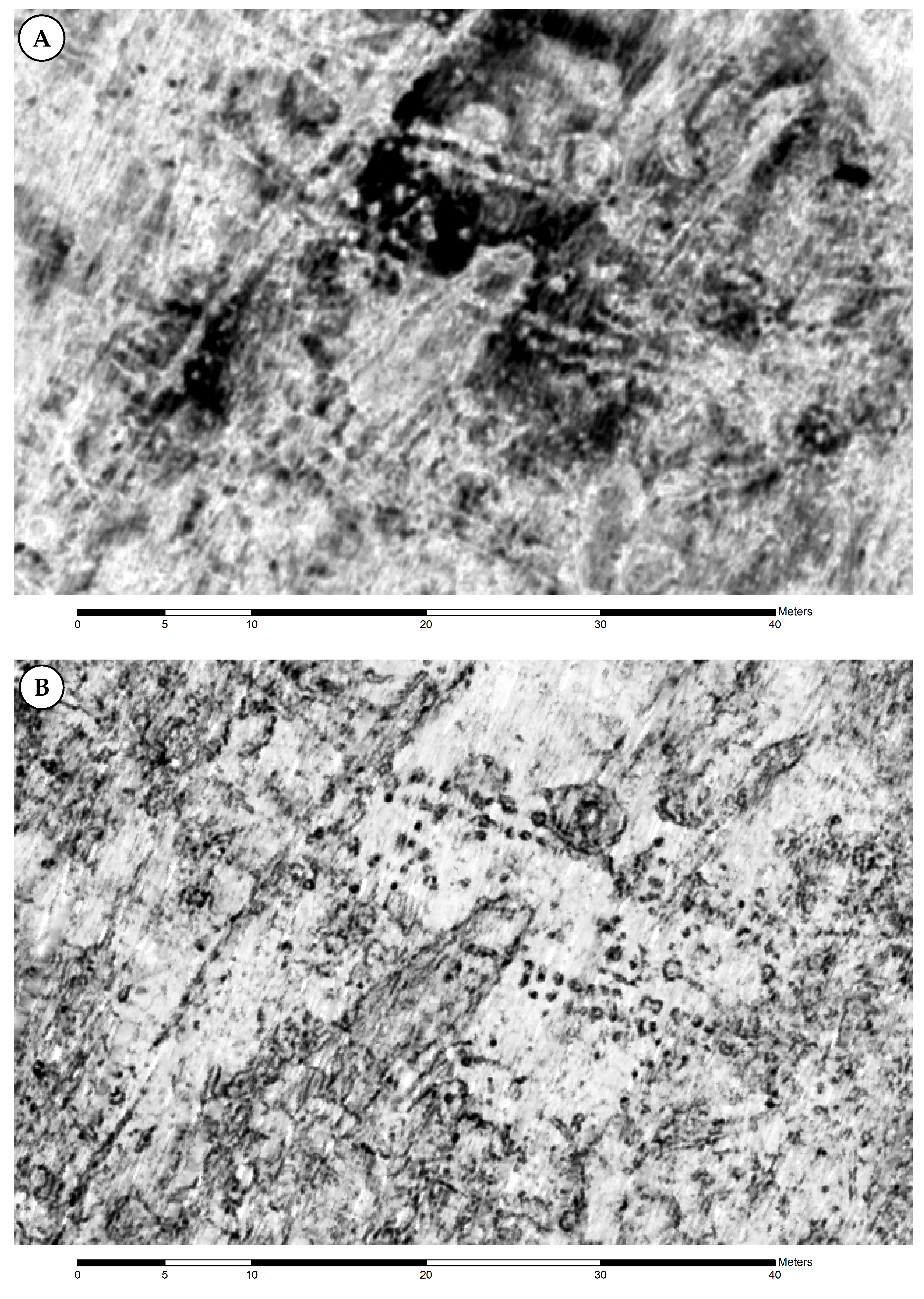
Stadil Mølleby (detail): Migrated GPR depth-slices from 55–85 cm depth showing the same area. (A) Conventional reflection amplitude map. (B) Inline coherence image. Note the rows of pits indicating building remains clearly visible in the coherence image.
Figure 6.
Stadil Mølleby (detail): Migrated GPR depth-slices from 55–85 cm depth showing the same area. (A) Conventional reflection amplitude map. (B) Inline coherence image. Note the rows of pits indicating building remains clearly visible in the coherence image.

Figure 7.
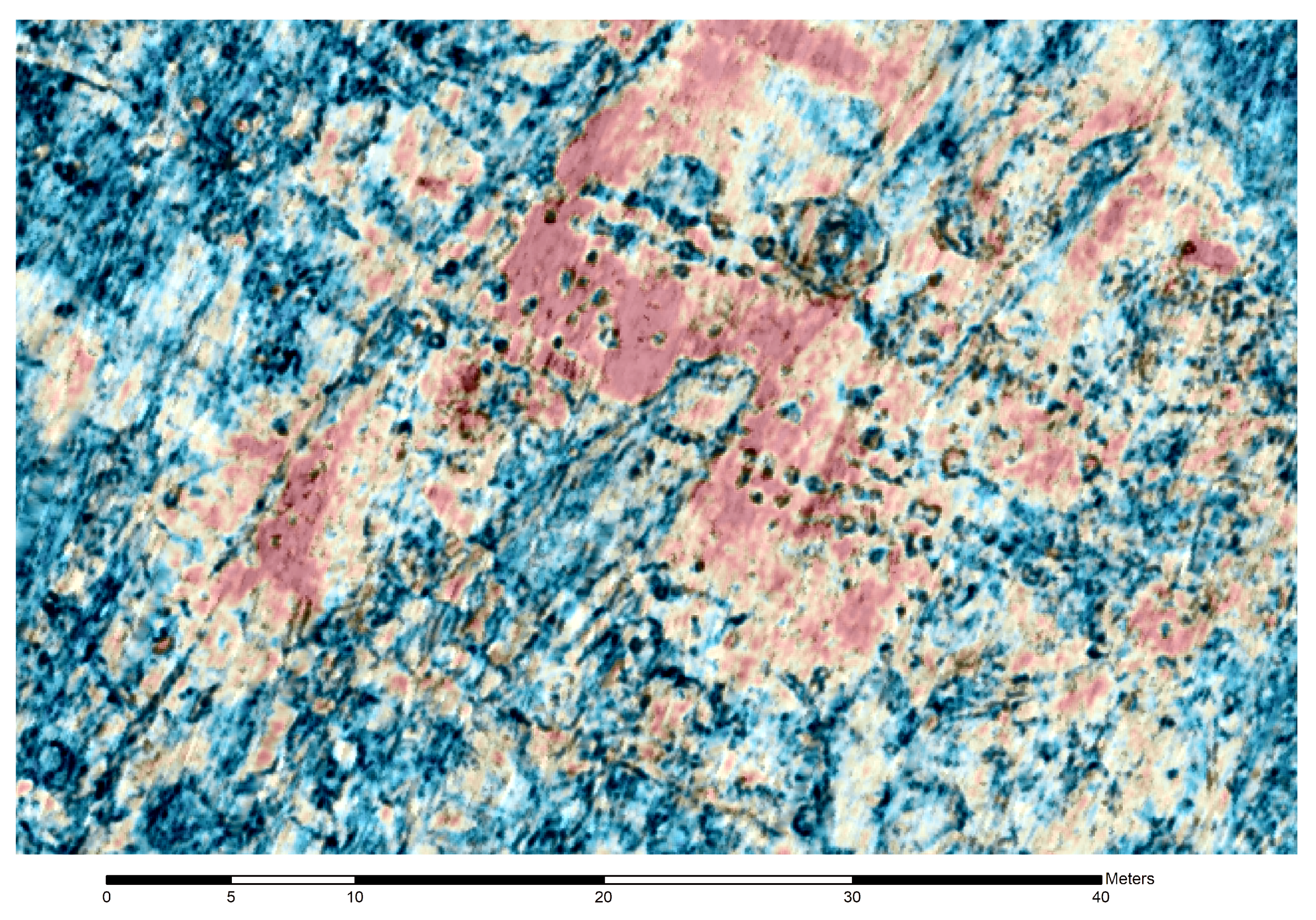
Stadil Mølleby (detail): Fused data image through normal fusion with an alpha value of 0.4 for the top image Figure 6A with seismic colour scale onto Figure 6B. Subsequently, histogram stretching was applied to bring out the details expressed by the black incoherence anomalies. The simple data fusion presented here is one way to merge two data images for ease of comprehension of the different information contained in each data set. The fused image preserved the crispness of the coherence anomalies, while adding the information on the higher reflective horizon marked by the red colour, into which apparently pits or postholes of a building have been dug. This fused image permits the joint simultaneous interpretation of the two complementary GPR amplitude and coherency data images.
Figure 7.
Stadil Mølleby (detail): Fused data image through normal fusion with an alpha value of 0.4 for the top image Figure 6A with seismic colour scale onto Figure 6B. Subsequently, histogram stretching was applied to bring out the details expressed by the black incoherence anomalies. The simple data fusion presented here is one way to merge two data images for ease of comprehension of the different information contained in each data set. The fused image preserved the crispness of the coherence anomalies, while adding the information on the higher reflective horizon marked by the red colour, into which apparently pits or postholes of a building have been dug. This fused image permits the joint simultaneous interpretation of the two complementary GPR amplitude and coherency data images.

Figure 8.
Four visualisations of GPR depth-slices (approx. 51.5 cm depth) from the overploughed burial mound with the remains of the Gjellestad Viking ship. North is upwards. (A) Standard amplitude map after Hilbert transformation. Light areas indicate absorbing structures, dark areas increased reflectivity. (B) Single-sample full amplitude slice. (C) Inverse image of (A). (D) Coherence map.

Figure 9.
Depth range 40–45 cm. (a) Unmigrated amplitude values. (b) Migrated amplitude values. (c) Inline coherence migrated. (d) Crossline coherence migrated. (e) In+crossline coherence migrated. (f) In+crossline coherence unmigrated.
Figure 9.
Depth range 40–45 cm. (a) Unmigrated amplitude values. (b) Migrated amplitude values. (c) Inline coherence migrated. (d) Crossline coherence migrated. (e) In+crossline coherence migrated. (f) In+crossline coherence unmigrated.

Figure 10.
Coherence computation using different cross-correlation lengths: (a) 1/4 wavelength, (b) 1/2 wavelength, (c) 1 wavelength, (d) 2 wavelengths, (e) 3 wavelengths, (f) 4 wavelengths.
Figure 10.
Coherence computation using different cross-correlation lengths: (a) 1/4 wavelength, (b) 1/2 wavelength, (c) 1 wavelength, (d) 2 wavelengths, (e) 3 wavelengths, (f) 4 wavelengths.

Figure 11.
Coherence data after subtraction of the average trace (AT) determined over different distance ranges: (a) no AT filter applied, (b) with 80 m AT filter, (c) with 40 m AT filter, (d) with 20 m AT filter, (e) with 10 m AT filter, (f) with 5 m AT filter.
Figure 11.
Coherence data after subtraction of the average trace (AT) determined over different distance ranges: (a) no AT filter applied, (b) with 80 m AT filter, (c) with 40 m AT filter, (d) with 20 m AT filter, (e) with 10 m AT filter, (f) with 5 m AT filter.

© 2020 by the authors. Licensee MDPI, Basel, Switzerland. This article is an open access article distributed under the terms and conditions of the Creative Commons Attribution (CC BY) license (http://creativecommons.org/licenses/by/4.0/).
Share and Cite
MDPI and ACS Style
Trinks, I.; Hinterleitner, A. Beyond Amplitudes: Multi-Trace Coherence Analysis for Ground-Penetrating Radar Data Imaging. Remote Sens. 2020, 12, 1583. https://0-doi-org.brum.beds.ac.uk/10.3390/rs12101583
AMA Style
Trinks I, Hinterleitner A. Beyond Amplitudes: Multi-Trace Coherence Analysis for Ground-Penetrating Radar Data Imaging. Remote Sensing. 2020; 12(10):1583. https://0-doi-org.brum.beds.ac.uk/10.3390/rs12101583
Chicago/Turabian StyleTrinks, Immo, and Alois Hinterleitner. 2020. "Beyond Amplitudes: Multi-Trace Coherence Analysis for Ground-Penetrating Radar Data Imaging" Remote Sensing 12, no. 10: 1583. https://0-doi-org.brum.beds.ac.uk/10.3390/rs12101583
Note that from the first issue of 2016, this journal uses article numbers instead of page numbers. See further details here.