Local Population Mapping Using a Random Forest Model Based on Remote and Social Sensing Data: A Case Study in Zhengzhou, China

 , , and
Abstract
:
1. Introduction
2. Methods
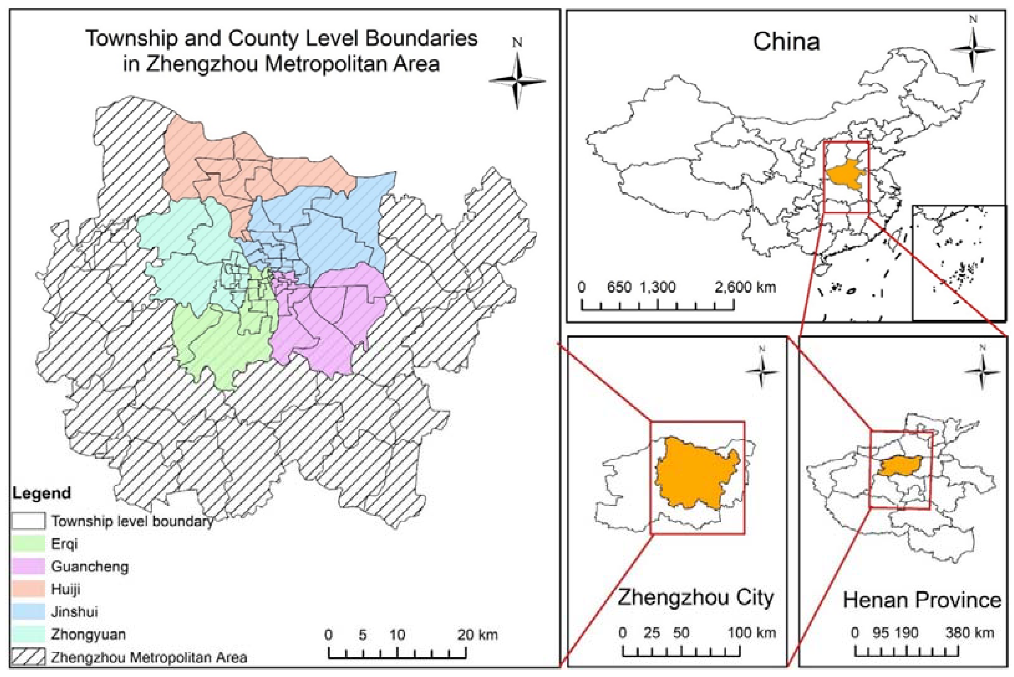
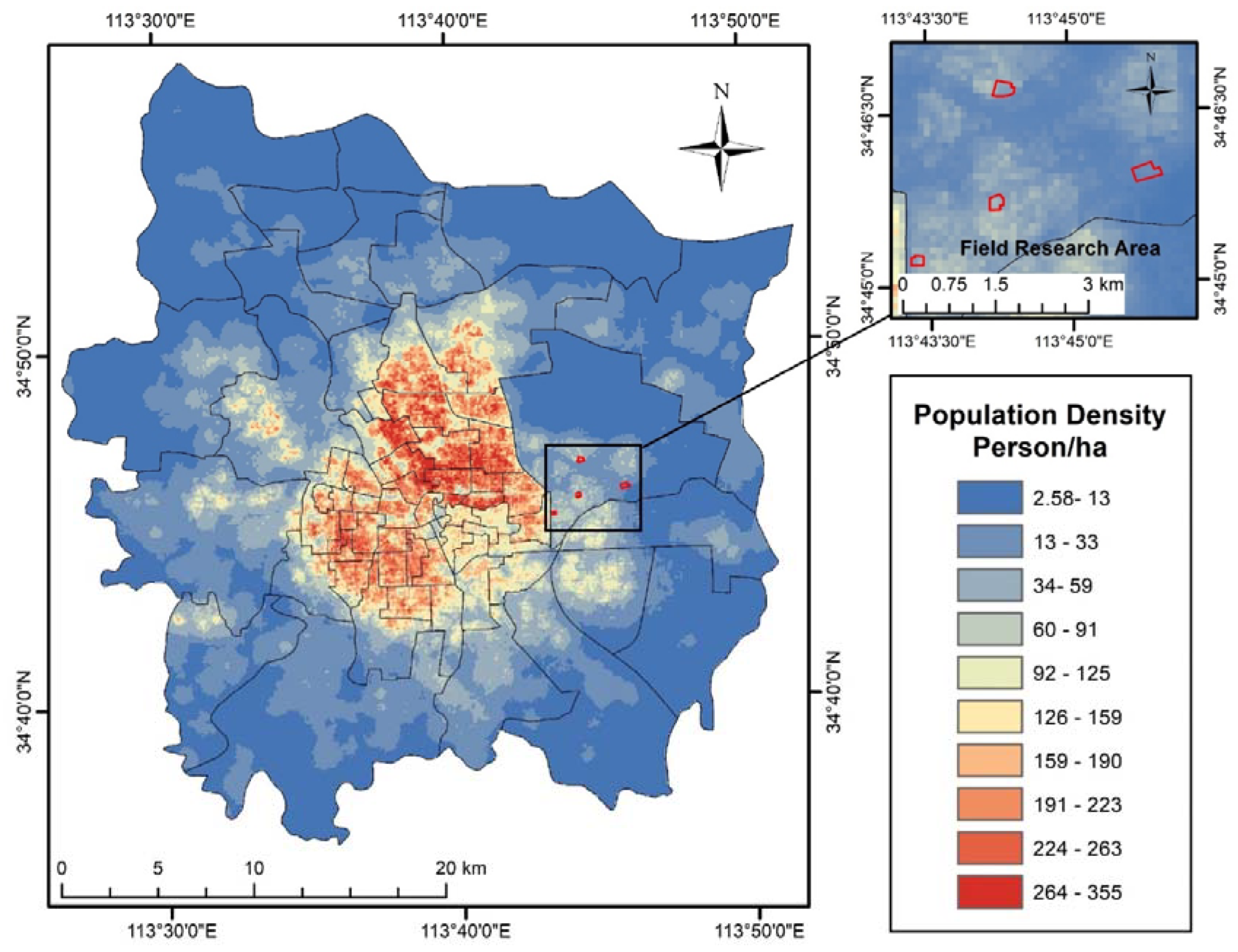
2.1. Study Area
2.2. Datasets
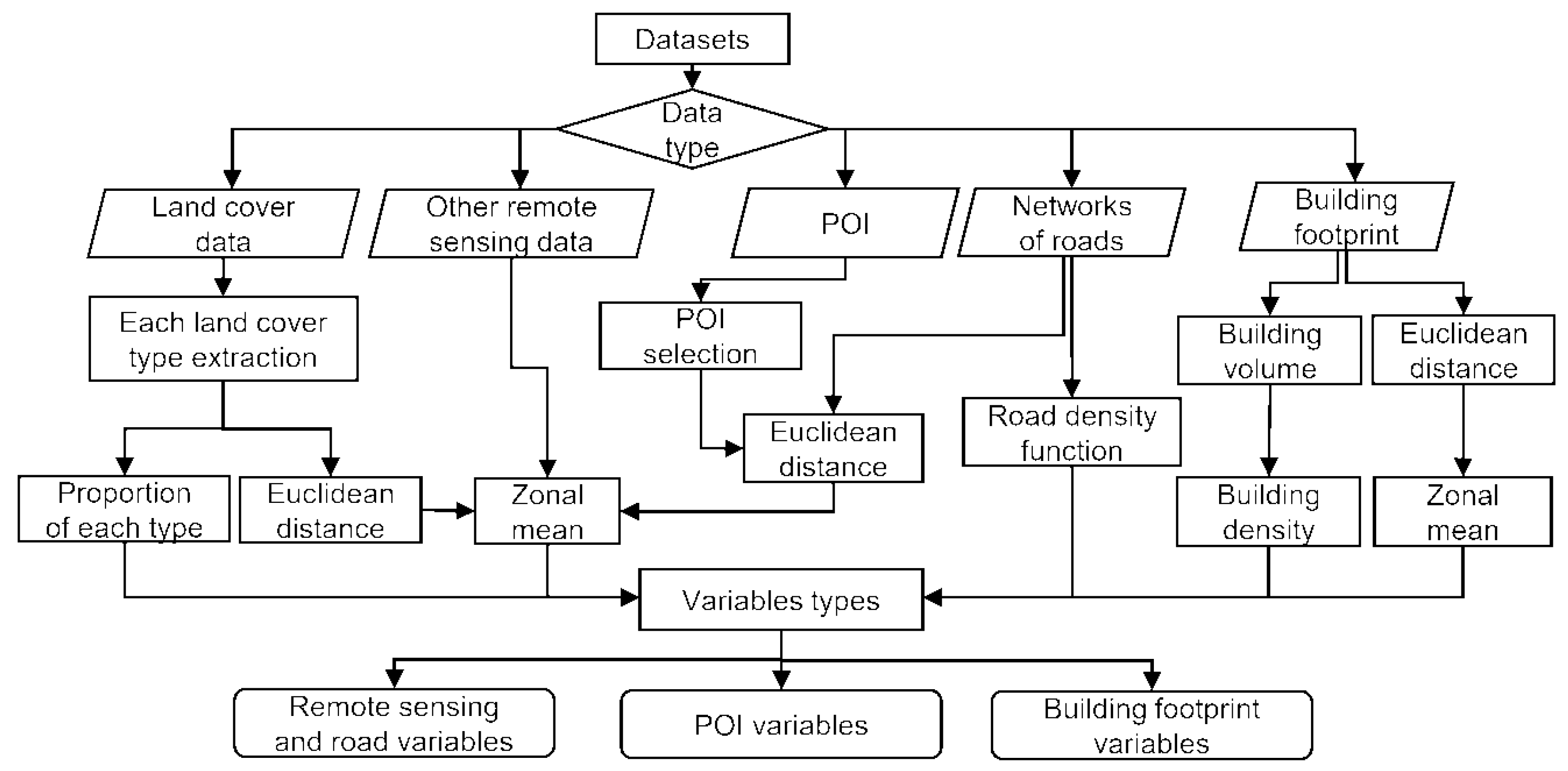
2.3. Data Preparation
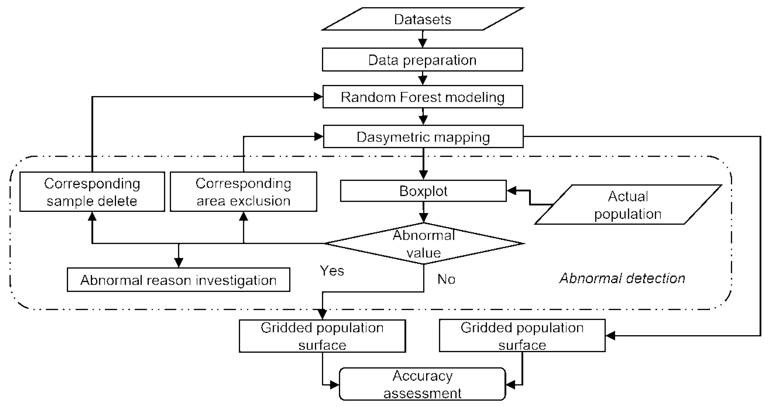
2.4. Population Modeling
2.4.1. Random Forest Model
2.4.2. Dasymetric Mapping
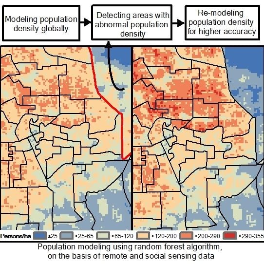
2.4.3. Abnormal Detection
2.4.4. Accuracy Assessment
3. Results
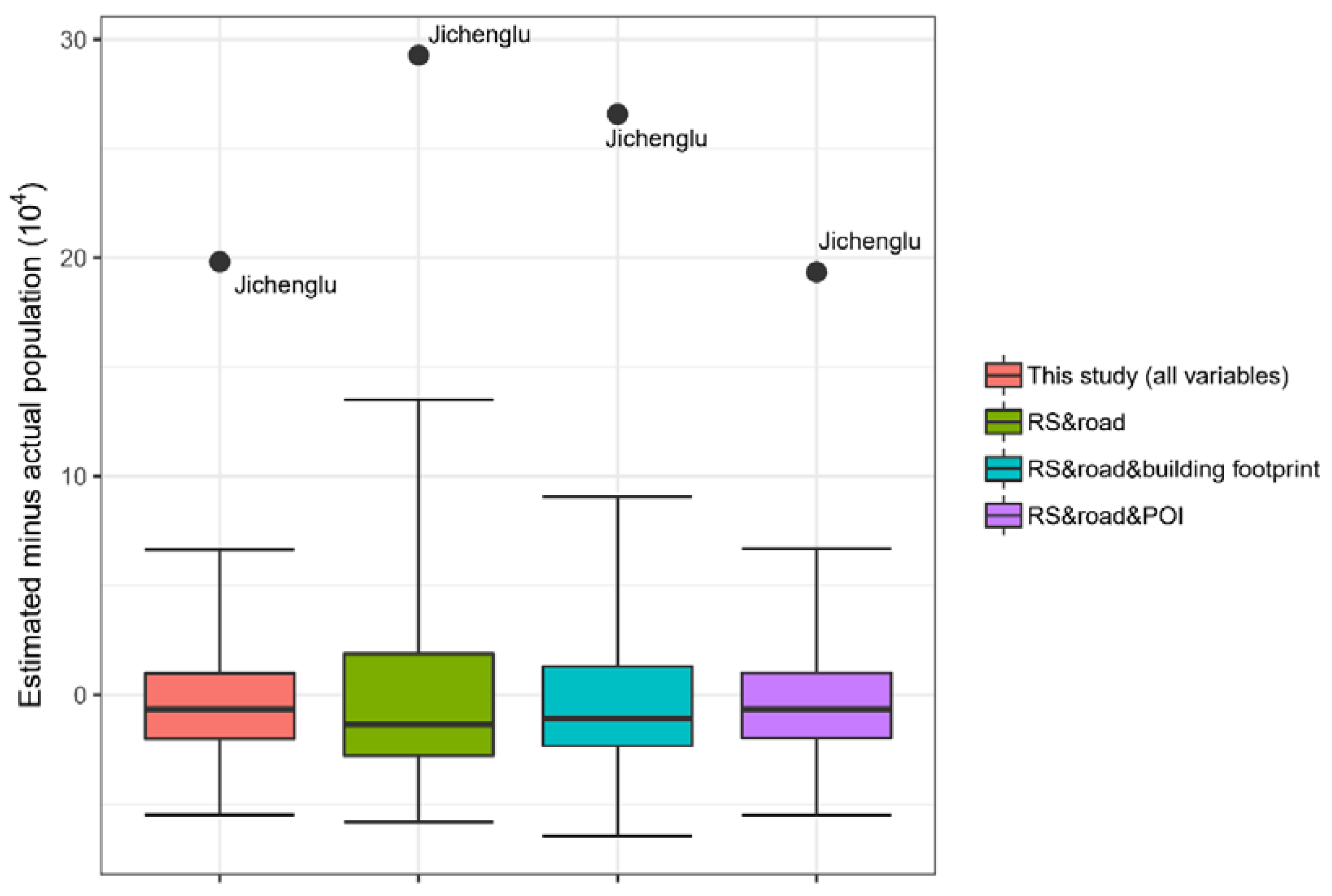
3.1. Abnormal Detection
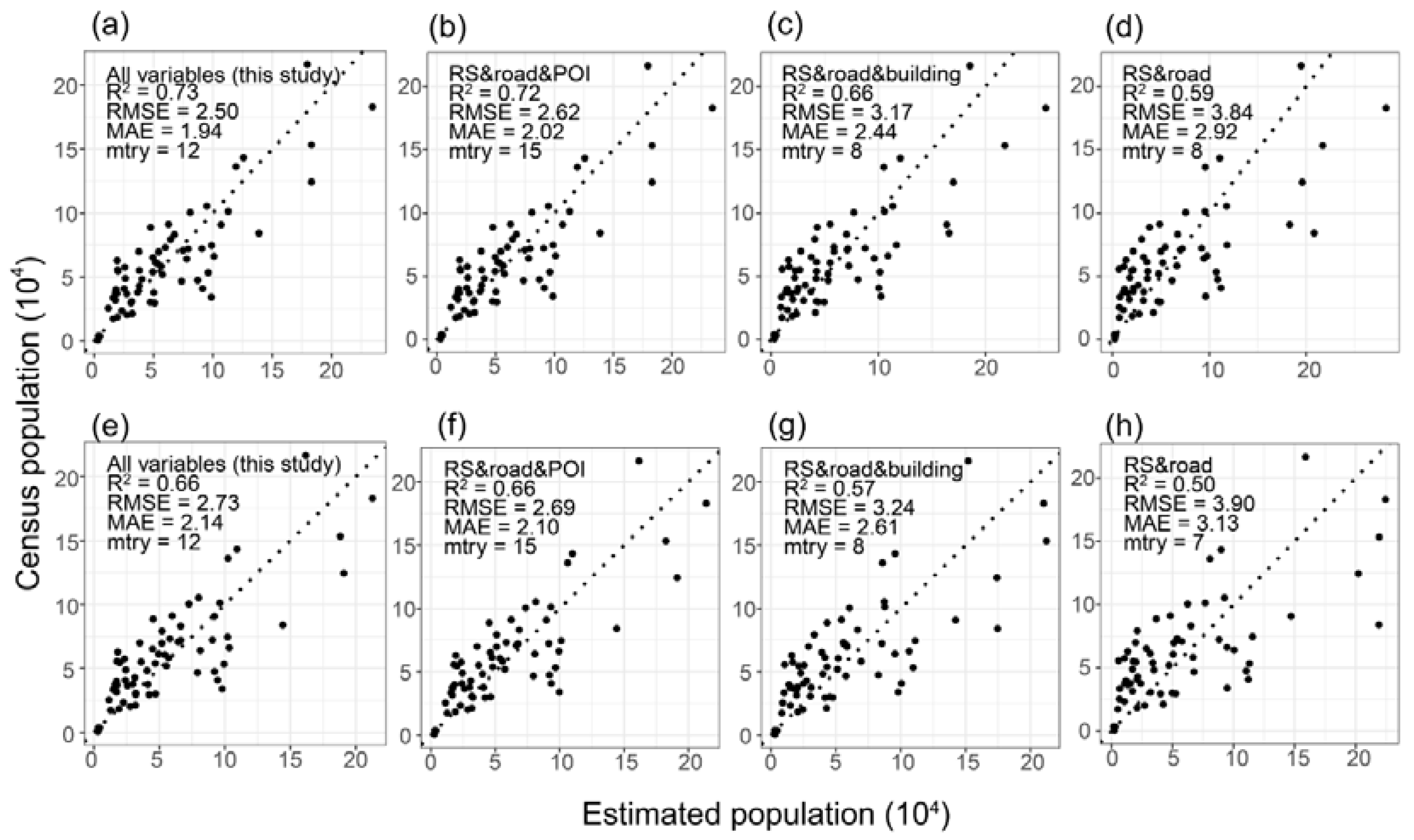
3.2. Accuracy Assessment
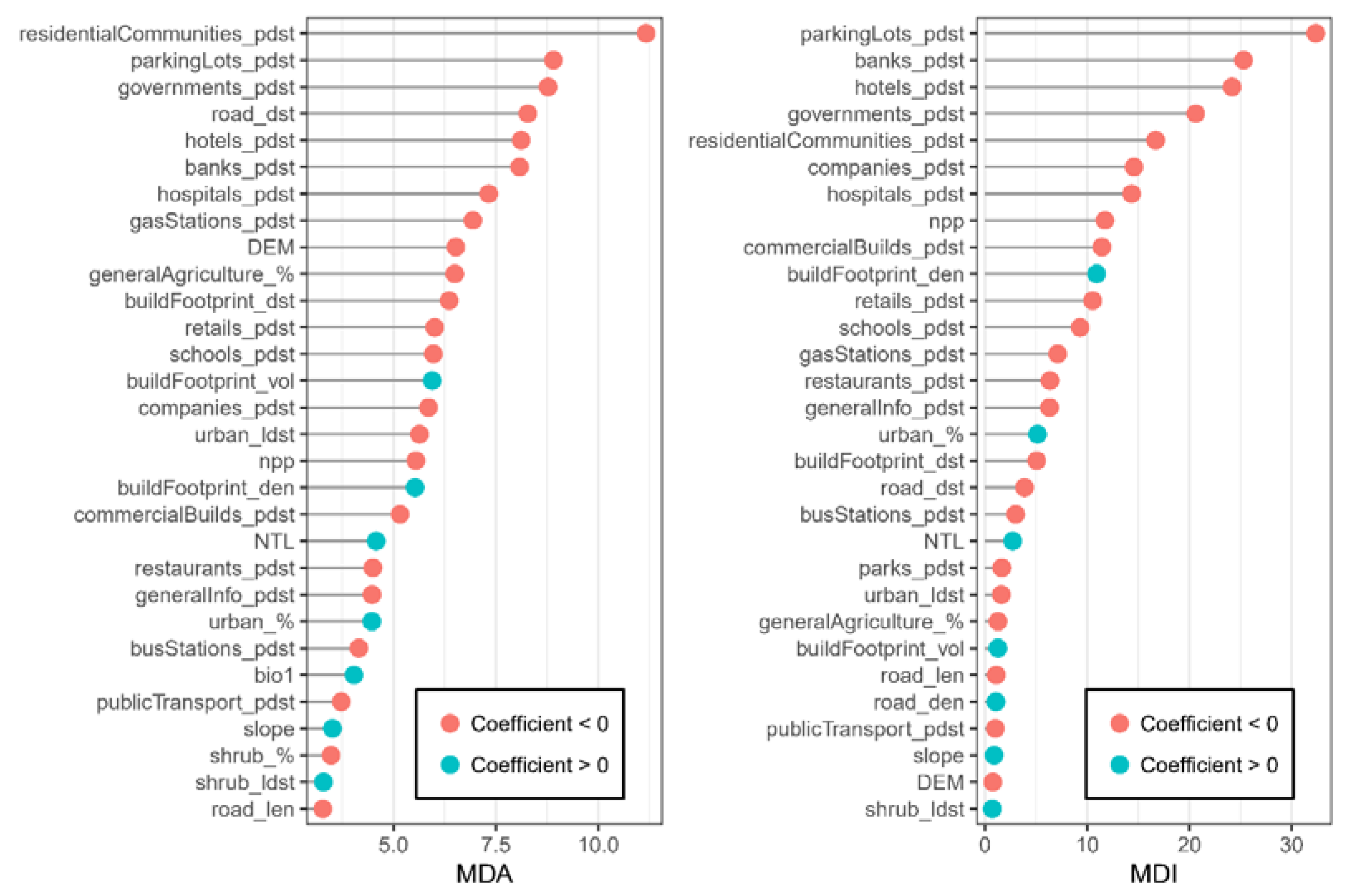
3.3. Variable Importance
4. Discussion
5. Conclusions
Author Contributions
Funding
Acknowledgments
Conflicts of Interest
References
- Azar, D.; Engstrom, R.; Graesser, J.; Comenetz, J. Generation of fine-scale population layers using multi-resolution satellite imagery and geospatial data. Remote Sens. Environ. 2013, 130, 219–232. [Google Scholar] [CrossRef]
- Jia, P.; Qiu, Y.; Gaughan, A.E. A fine-scale spatial population distribution on the High-resolution Gridded Population Surface and application in Alachua County, Florida. Appl. Geogr. 2014, 50, 99–107. [Google Scholar] [CrossRef]
- Dobson, J.E.; Bright, E.A.; Coleman, P.R.; Durfee, R.C.; Worley, B.A. LandScan: A global population database for estimating populations at risk. Photogramm. Eng. Remote Sens. 2000, 66, 849–857. [Google Scholar]
- Jia, P.; Anderson, J.D.; Leitner, M.; Rheingans, R. High-resolution spatial distribution and estimation of access to improved sanitation in Kenya. PLoS ONE 2016, 11, e0158490. [Google Scholar] [CrossRef] [Green Version]
- Elvidge, C.D.; Baugh, K.E.; Kihn, E.A.; Kroehl, H.W.; Davis, E.R.; Davis, C.W. Relation between satellite observed visible-near infrared emissions, population, economic activity and electric power consumption. Int. J. Remote Sens. 1997, 18, 1373–1379. [Google Scholar] [CrossRef]
- Zhang, N.; Huang, H.; Su, B.; Zhang, H. Population evacuation analysis: Considering dynamic population vulnerability distribution and disaster information dissemination. Nat. Hazards 2013, 69, 1629–1646. [Google Scholar] [CrossRef]
- Wilson, R.; Erbachschoenberg, E.Z.; Albert, M.; Power, D.; Tudge, S.; Gonzalez, M.; Guthrie, S.; Chamberlain, H.; Brooks, C.; Hughes, C. Rapid and Near Real-Time Assessments of Population Displacement Using Mobile Phone Data Following Disasters: The 2015 Nepal Earthquake. PLoS Curr. 2016, 8. [Google Scholar] [CrossRef]
- Jia, P.; Shi, X.Y.; Xierali, I.M. Teaming up census and patient data to delineate fine-scale hospital service areas and identify geographic disparities in hospital accessibility. Environ. Monit. Assess. 2019, 191, 303. [Google Scholar] [CrossRef] [Green Version]
- Jia, P.; Wang, F.H.; Xierali, I.M. Differential effects of distance decay on hospital inpatient visits among subpopulations in Florida, USA. Environ. Monit. Assess. 2019, 191, 381. [Google Scholar] [CrossRef] [Green Version]
- Mennis, J. Generating Surface Models of Population Using Dasymetric Mapping. Prof. Geogr. 2003, 55, 31–42. [Google Scholar]
- Yi, G.; Hui, W.; Wang, P. Population Spatial Processing for Chinese Coastal Zones Based on Census and Multiple Night Light Data. Resour. Sci. 2013, 35, 2517–2523. [Google Scholar]
- Martin, D. Directions in population GIS. Geogr. Compass. 2011, 5, 655–665. [Google Scholar] [CrossRef]
- Tobler, W.; Deichmann, U.; Gottsegen, J.; Maloy, K. World population in a grid of spherical quadrilaterals. Int. J. Popul. Geogr. 1997, 3, 203–225. [Google Scholar] [CrossRef]
- Tobler, W.R. Smooth Pycnophylactic Interpolation for Geographical Regions. J. Am. Stat. Assoc. 1979, 74, 519–530. [Google Scholar] [CrossRef]
- Langford, M.; Harvey, J.T. The Use of Remotely Sensed Data for Spatial Disaggregation of Published Census Population Counts. In Proceedings of the IEEE/ISPRS Joint Workshop on Remote Sensing and Data Fusion over Urban Areas, DFUA 2001, Rome, Italy, 8–9 November 2001; pp. 260–264. [Google Scholar]
- Zhou, C.; Yang, O.U.; Ting, M.A. Progresses of Geographical Grid Systems Researches. Prog. Geogr. 2009, 28, 657–662. [Google Scholar]
- Balk, D.; Yetman, G. The Global Distribution of Population: Evaluating the Gains in Resolution Refinement; Center for International Earth Science Information Network (CIESIN), Columbia University: New York, NY, USA, 2004. [Google Scholar]
- Balk, D.L.; Deichmann, U.; Yetman, G.; Pozzi, F.; Hay, S.I.; Nelson, A. Determining Global Population Distribution: Methods, Applications and Data. Adv. Parasitol. 2006, 62, 119–156. [Google Scholar]
- Freire, S.; Doxsey-Whitfield, E.; MacManus, K.; Mills, J.; Pesaresi, M. Development of new open and free multi-temporal global population grids at 250 m resolution. Population 2000, 250. [Google Scholar]
- Stevens, F.R.; Gaughan, A.E.; Linard, C.; Tatem, A.J. Disaggregating census data for population mapping using random forests with remotely-sensed and ancillary data. PLoS ONE 2015, 10, e0107042. [Google Scholar] [CrossRef] [Green Version]
- Leyk, S.; Gaughan, A.E.; Adamo, S.B.; de Sherbinin, A.; Balk, D.; Freire, S.; Rose, A.; Stevens, F.R.; Blankespoor, B.; Frye, C.; et al. The spatial allocation of population: A review of large-scale gridded population data products and their fitness for use. Earth Syst. Sci. Data 2019, 11, 1385–1409. [Google Scholar] [CrossRef] [Green Version]
- Linard, C.; Gilbert, M.; Tatem, A.J.J.G. Assessing the use of global land cover data for guiding large area population distribution modelling. GeoJournal 2011, 76, 525–538. [Google Scholar] [CrossRef] [Green Version]
- Cohen, J.E.; Small, C. Hypsographic demography: The distribution of human population by altitude. Proc. Natl. Acad. Sci. USA 1998, 95, 14009–14014. [Google Scholar] [CrossRef] [PubMed] [Green Version]
- Ye, T.T.; Zhao, N.Z.; Yang, X.C.; Ouyang, Z.T.; Liu, X.P.; Chen, Q.; Hu, K.J.; Yue, W.Z.; Qi, J.G.; Li, Z.S.; et al. Improved population mapping for China using remotely sensed and points-of-interest data within a random forests model. Sci. Total Environ. 2019, 658, 936–946. [Google Scholar] [CrossRef] [PubMed]
- Sutton, P.; Roberts, D.; Elvidge, C.; Baugh, K. Census from Heaven: An estimate of the global human population using night-time satellite imagery. In. J. Remote Sens. 2001, 22, 3061–3076. [Google Scholar] [CrossRef]
- Briggs, D.J.; Gulliver, J.; Fecht, D.; Vienneau, D.M. Dasymetric modelling of small-area population distribution using land cover and light emissions data. Remote Sens. Environ. 2007, 108, 451–466. [Google Scholar] [CrossRef]
- Alahmadi, M.; Atkinson, P.M.; Martin, D. A Comparison of Small-Area Population Estimation Techniques Using Built-Area and Height Data, Riyadh, Saudi Arabia. IEEE J. Sel. Top. Appl. Earth Obs. Remote Sens. 2016, 9, 1959–1969. [Google Scholar] [CrossRef]
- Roni, R.; Jia, P. An Optimal Population Modeling Approach Using Geographically Weighted Regression Based on High-Resolution Remote Sensing Data: A Case Study in Dhaka City, Bangladesh. Remote Sens. 2020, 12, 1184. [Google Scholar] [CrossRef] [Green Version]
- Bakillah, M.; Liang, S.; Mobasheri, A.; Arsanjani, J.J.; Zipf, A. Fine-resolution population mapping using OpenStreetMap points-of-interest. Int. J. Geogr. Inf. Sci. 2014, 28, 1940–1963. [Google Scholar] [CrossRef]
- Yang, X.C.; Ye, T.T.; Zhao, N.Z.; Chen, Q.; Yue, W.Z.; Qi, J.G.; Zeng, B.; Jia, P. Population Mapping with Multisensor Remote Sensing Images and Point-Of-Interest Data. Remote Sens. 2019, 11, 574. [Google Scholar] [CrossRef] [Green Version]
- Belgiu, M.; Drăguţ, L. Random forest in remote sensing: A review of applications and future directions. ISPRS J. Photogramm. Remote Sens. 2016, 114, 24–31. [Google Scholar] [CrossRef]
- Breiman, L. Random Forests. Mach. Learn. 2001, 45, 5–32. [Google Scholar] [CrossRef] [Green Version]
- Tatem, A.J.; Gaughan, A.E.; Stevens, F.R.; Patel, N.N.; Jia, P.; Pandey, A.; Linard, C. Quantifying the effects of using detailed spatial demographic data on health metrics: A systematic analysis for the AfriPop, AsiaPop, and AmeriPop projects. Lancet 2013, 381, S142. [Google Scholar] [CrossRef]
- Tan, M.; Liu, K.; Liu, L.; Zhu, Y.; Wang, D. Spatialization of population in the Pearl River Delta in 30 m grids using random forest model. Prog. Geogr. 2017, 36, 1304–1312. [Google Scholar]
- Fu, J.; Jiang, D.; Huang, Y. 1 km grid population dataset of China (2005, 2010). Acta Geogr. Sin. 2014, 69, 136–139. [Google Scholar] [CrossRef]
- Census Office; Department of Population and Employment Statistics. China 2010 Population Census Information; China Statistics Press: Beijing, China, 2012. [Google Scholar]
- Lo, C.P. Raster approach to population estimation using high-altitude aerial and space photographs. Remote Sens. Environ. 1989, 27, 59–71. [Google Scholar] [CrossRef]
- Tatem, A.J.; Noor, A.M.; Von Hagen, C.; Di Gregorio, A.; Hay, S.I. High resolution population maps for low income nations: Combining land cover and census in East Africa. PLoS ONE 2007, 2, e1298. [Google Scholar] [CrossRef]
- Luck, G.W. The relationships between net primary productivity, human population density and species conservation. J. Biogeogr. 2007, 34, 201–212. [Google Scholar] [CrossRef]
- Running, S.W.; Nemani, R.R.; Heinsch, F.A.; Zhao, M.S.; Reeves, M.; Hashimoto, H. A continuous satellite-derived measure of global terrestrial primary production. Bioscience 2004, 54, 547–560. [Google Scholar] [CrossRef]
- Walsh, S.J.; Evans, T.P.; Welsh, W.F.; Entwisle, B.; Rindfuss, R.R. Scale-dependent relationships between population and environment in northeastern Thailand. Photogramm. Eng. Remote Sens. 1999, 65, 97. [Google Scholar]
- Hijmans, R.J.; Cameron, S.E.; Parra, J.L.; Jones, P.G.; Jarvis, A. Very high resolution interpolated climate surfaces for global land areas. Int. J. Clim. 2010, 25, 1965–1978. [Google Scholar] [CrossRef]
- Lo, C. Urban indicators of china from radiance-calibrated digital dmsp-ols nighttime images. Ann. Assoc. Am. Geogr. 2002, 92, 225–240. [Google Scholar] [CrossRef]
- Elvidge, C.D.; Baugh, K.E.; Zhizhin, M.; Hsu, F.-C. Why VIIRS data are superior to DMSP for mapping nighttime lights. Proc. Asia Pac. Adv. Netw. 2013, 35, 62. [Google Scholar] [CrossRef] [Green Version]
- Liu, X.; He, J.; Yao, Y.; Zhang, J.; Liang, H.; Wang, H.; Hong, Y. Classifying urban land use by integrating remote sensing and social media data. Int. J. Geogr. Inf. Sci. 2017, 31, 1675–1696. [Google Scholar] [CrossRef]
- Wang, S.; Tian, Y.; Zhou, Y.; Liu, W.; Lin, C. Fine-scale population estimation by 3D reconstruction of urban residential buildings. Sensors 2016, 16, 1755. [Google Scholar] [CrossRef] [Green Version]
- Tomás, L.; Fonseca, L.; Almeida, C.; Leonardi, F.; Pereira, M. Urban population estimation based on residential buildings volume using IKONOS-2 images and lidar data. Int. J. Remote Sens. 2016, 37, 1–28. [Google Scholar] [CrossRef] [Green Version]
- Zhang, C.Y.; Qiu, F. A Point-Based Intelligent Approach to Areal Interpolation. Prof. Geogr. 2011, 63, 262–276. [Google Scholar] [CrossRef]
- Bai, Z.; Wang, J.; Yang, Y.; Sun, J. Characterizing spatial patterns of population distribution at township level across the 25 provinces in China. Acta Geogr. Sin. 2015, 70, 1229–1242. [Google Scholar]
- Liaw, A.; Wiener, M. Classification and Regression by randomForest. R. News 2013, 2, 18–22. [Google Scholar]
- Hur, J.-H.; Ihm, S.-Y.; Park, Y.-H. A Variable Impacts Measurement in Random Forest for Mobile Cloud Computing. Wirel. Commun. Mob. Comput. 2017, 2017, 6817627. [Google Scholar] [CrossRef] [Green Version]
- Strobl, C.; Boulesteix, A.L.; Zeileis, A.; Hothorn, T. Bias in random forest variable importance measures: Illustrations, sources and a solution. BMC Bioinform. 2007, 8, 25. [Google Scholar] [CrossRef] [Green Version]
- Pal, M. Random forest classifier for remote sensing classification. Int. J. Remote Sens. 2005, 26, 217–222. [Google Scholar] [CrossRef]
- He, L.; Levine, R.A.; Fan, J.; Beemer, J.; Stronach, J. Random forest as a predictive analytics alternative to regression in institutional research. Pract. Assess. Res. Eval. 2018, 23, 1. [Google Scholar]
- Williamson, D.F.; Parker, R.A.; Kendrick, J.S. The box plot: A simple visual method to interpret data. Ann. Intern. Med. 1989, 110, 916–921. [Google Scholar] [CrossRef] [PubMed]
- Frigge, M.; Hoaglin, D.C.; Iglewicz, B. Some implementations of the boxplot. Am. Stat. 1989, 43, 50–54. [Google Scholar] [CrossRef]
- Tukey, J.W. Exploratory Data Analysis: Limited Preliminary Ed; Addison-Wesley Publishing Company: Ann Arbor, MI, USA, 1970. [Google Scholar]
- Liu, X.; Kyriakidis, P.C.; Goodchild, M.F. Population-density estimation using regression and area-to-point residual kriging. Int. J. Geogr. Inf. Sci. 2008, 22, 431–447. [Google Scholar] [CrossRef]
- Langford, M. An evaluation of small area population estimation techniques using open access ancillary data. Geogr. Anal. 2013, 45, 324–344. [Google Scholar] [CrossRef]
- State Council of The People’s Republic of China. Gazette of the State Council of The People’s Republic of China; The State Council of The People’s Republic of China, Ed.; General Office of The State Council of The People’s Republic of China: Beijing, China, 1998; pp. 1004–3438.
- Niu, J. Research on the Countermeasures for the Healthy Development of Commercial Housing Market in Zhengzhou City. China Mark. 2015, 176–183. [Google Scholar] [CrossRef]
- Guo, S. About Empty City, Vacancy and Housing Vacancy Rate. City House 2012, 37–38. [Google Scholar]
- Jacobsen, K.; Passini, R. Analsysis of ASTER GDEM Elevation Models. In Proceedings of the International Archives of the Photogrammetry, Remote Sensing and Spatial Information Sciences: [2010 Canadian Geomatics Conference And Symposium Of Commission I, ISPRS Convergence In Geomatics-Shaping Canada’s Competitive Landscape] 38 (2010), Nr. Part 1, Calgary, AB, Canada, 15–18 June 2010. [Google Scholar]
- Jia, P.; Gaughan, A.E. Dasymetric modeling: A hybrid approach using land cover and tax parcel data for mapping population in Alachua County, Florida. Appl. Geogr. 2016, 66, 100–108. [Google Scholar] [CrossRef]
- Zhang, J.L.; Xu, W.; Qin, L.J.; Tian, Y.G. Spatial Distribution Estimates of the Urban Population Using DSM and DEM Data in China. ISPRS Int. J. Geo-Inf. 2018, 7, 435. [Google Scholar] [CrossRef] [Green Version]
- Haklay, M.; Weber, P. Openstreetmap: User-generated street maps. IEEE Pervas. Comput. 2008, 7, 12–18. [Google Scholar] [CrossRef] [Green Version]
- Sinha, P.; Gaughan, A.E.; Stevens, F.R.; Nieves, J.J.; Sorichetta, A.; Tatem, A.J. Assessing the spatial sensitivity of a random forest model: Application in gridded population modeling. Comput. Environ. Urban Syst. 2019, 75, 132–145. [Google Scholar] [CrossRef]


| Data | Description | Year | Source |
|---|---|---|---|
| Raster data (remote sensing data) | |||
| BaseVue 2013 landcover data | A 30 m spatial resolution global land cover dataset containing 14 types of land cover, including water, wetland, general agricultural land, paddy agricultural land, urban, etc. | 2013 | MDA Information Systems LLC., USA |
| MOD17A3 NPP data | A 1 km MODIS annual product that provides an accurate measure of the net primary productivity of terrestrial vegetation | 2010 | National Aeronautics and Space Administration (NASA), USA |
| VIIRS 2012 night-time lights data | 500 m resolution lights at night that exclude fires and other ephemeral lights | 2012 | National Oceanic and Atmospheric Administration (NOAA), USA |
| ASTER GDEM Version 2 data | A global effort that provides 30 m resolution elevation information | - | United States Geological Survey (USGS), USA |
| WorldClim Version2 temperature data | A global dataset that measured mean temperatures from 1970 to 2000 | 1970–2000 | The Feed the Future Innovation Lab for Collaborative Research on Sustainable Intensification (SIIL), USA |
| WorldClim Version2 precipitation data | A global dataset that measured mean precipitation from 1970 to 2000 | 1970–2000 | The Feed the Future Innovation Lab for Collaborative Research on Sustainable Intensification (SIIL), USA |
| Vector data (social sensing data) | |||
| Boundary maps | Township and county Level Administrative Boundaries | 2010 | Henan Administration of Surveying Mapping and Geoinformation, China |
| Road networks | Including railway, national road, provincial road, county road, and township road | 2018 | AutoNavi Software Co., Ltd., China |
| Point of interest | 20 categories including: residential communities, banks, parking lots, etc. | 2010 | Baidu Inc., China |
| Building footprint | Building footprints with height information | 2018 | AutoNavi Software Co., Ltd., China |
| RMSE | MAE | |
|---|---|---|
| This study | 24,956.93 | 19,420.04 |
| Worldpop | 31,543.66 | 22,687.94 |
| GPW | 33,791.59 | 26,132.49 |
| GPC | 35,800.90 | 29,074.32 |
© 2020 by the authors. Licensee MDPI, Basel, Switzerland. This article is an open access article distributed under the terms and conditions of the Creative Commons Attribution (CC BY) license (http://creativecommons.org/licenses/by/4.0/).
Share and Cite
Qiu, G.; Bao, Y.; Yang, X.; Wang, C.; Ye, T.; Stein, A.; Jia, P. Local Population Mapping Using a Random Forest Model Based on Remote and Social Sensing Data: A Case Study in Zhengzhou, China. Remote Sens. 2020, 12, 1618. https://0-doi-org.brum.beds.ac.uk/10.3390/rs12101618
Qiu G, Bao Y, Yang X, Wang C, Ye T, Stein A, Jia P. Local Population Mapping Using a Random Forest Model Based on Remote and Social Sensing Data: A Case Study in Zhengzhou, China. Remote Sensing. 2020; 12(10):1618. https://0-doi-org.brum.beds.ac.uk/10.3390/rs12101618
Chicago/Turabian StyleQiu, Ge, Yuhai Bao, Xuchao Yang, Chen Wang, Tingting Ye, Alfred Stein, and Peng Jia. 2020. "Local Population Mapping Using a Random Forest Model Based on Remote and Social Sensing Data: A Case Study in Zhengzhou, China" Remote Sensing 12, no. 10: 1618. https://0-doi-org.brum.beds.ac.uk/10.3390/rs12101618