Enhancing Methods for Under-Canopy Unmanned Aircraft System Based Photogrammetry in Complex Forests for Tree Diameter Measurement

Abstract

The application of Unmanned Aircraft Systems (UAS) beneath the forest canopy provides a potentially valuable alternative to ground-based measurement techniques in areas of dense canopy cover and undergrowth. This research presents results from a study of a consumer-grade UAS flown under the forest canopy in challenging forest and terrain conditions. This UAS was deployed to assess under-canopy UAS photogrammetry as an alternative to field measurements for obtaining stem diameters as well as ultra-high-resolution (~400,000 points/m²) 3D models of forest study sites. There were 378 tape-based diameter measurements collected from 99 stems in a native, unmanaged eucalyptus pulchella forest with mixed understory conditions and steep terrain. These measurements were used as a baseline to evaluate the accuracy of diameter measurements from under-canopy UAS-based photogrammetric point clouds. The diameter measurement accuracy was evaluated without the influence of a digital terrain model using an innovative tape-based method. A practical and detailed methodology is presented for the creation of these point clouds. Lastly, a metric called the Circumferential Completeness Index (CCI) was defined to address the absence of a clearly defined measure of point coverage when measuring stem diameters from forest point clouds. The measurement of the mean CCI is suggested for use in future studies to enable a consistent comparison of the coverage of forest point clouds using different sensors, point densities, trajectories, and methodologies. It was found that root-mean-squared-errors of diameter measurements were 0.011 m in Site 1 and 0.021 m in the more challenging Site 2. The point clouds in this study had a mean validated CCI of 0.78 for Site 1 and 0.7 for Site 2, with a mean unvalidated CCI of 0.86 for Site 1 and 0.89 for Site 2. The results in this study demonstrate that under-canopy UAS photogrammetry shows promise in becoming a practical alternative to traditional field measurements, however, these results are currently reliant upon the operator’s knowledge of photogrammetry and his/her ability to fly manually in object-rich environments. Future work should pursue solutions to autonomous operation, more complete point clouds, and a method for providing scale to point clouds when global navigation satellite systems are unavailable.

1. Introduction

With seemingly continuous advancements in remote sensing technologies, there is a following trend for forestry and conservation organizations to demand deeper understandings over larger-scale areas of forest than was previously possible using conventional field measurement techniques. Individual tree level inventories have been possible for some time with remote sensing techniques; however, further research and refinement is needed for these ultra-high-resolution systems to become practical for widespread application. Improving how forests are measured may help the forestry supply chain to extract more value from a given forest stand, as potential saw logs (high value), which may not be identified as such, may be turned into wood chips (low value) unnecessarily if information about the stand being harvested is of poor quality. It remains common practice for forest plots to be measured using measuring tapes, calipers, and similar basic tools, however, this is changing quickly.

Unmanned aerial systems (UAS) are increasingly being adopted for use in forestry and ecosystem monitoring applications due to their time efficiency, low operating costs, and wide-ranging applications [1,2]. There exists a considerable volume of research on flying UAS above forest canopies that provides evidence of their utility; however, it is commonly seen that where forest canopies are dense, forest under-story structures and individual stem characteristics are often occluded by the canopy [3,4,5]. A common work-around for this issue is to build models to relate ground-based field measurements to datasets acquired through aerial photogrammetry (AP) or aerial laser scanning (ALS) [6,7].

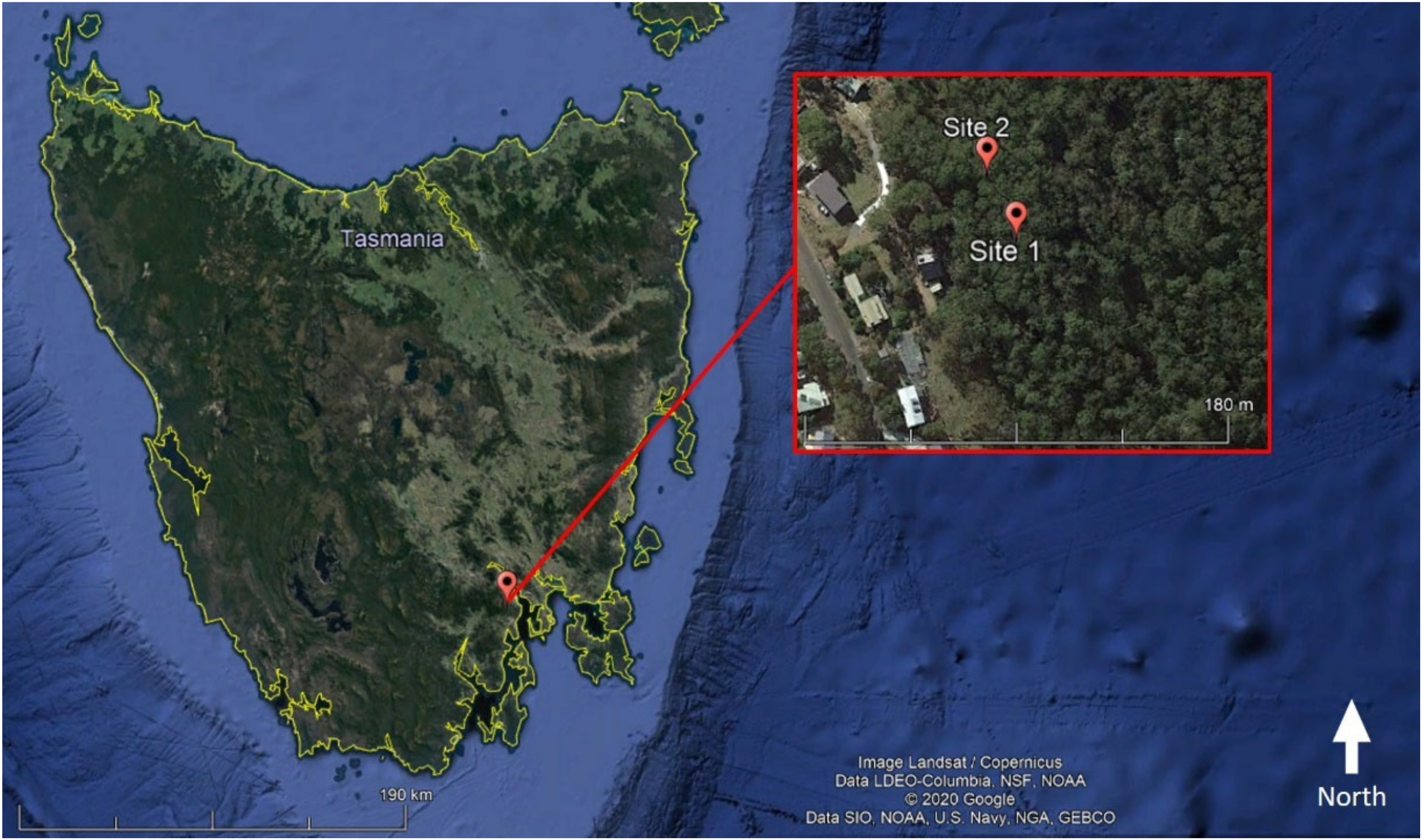
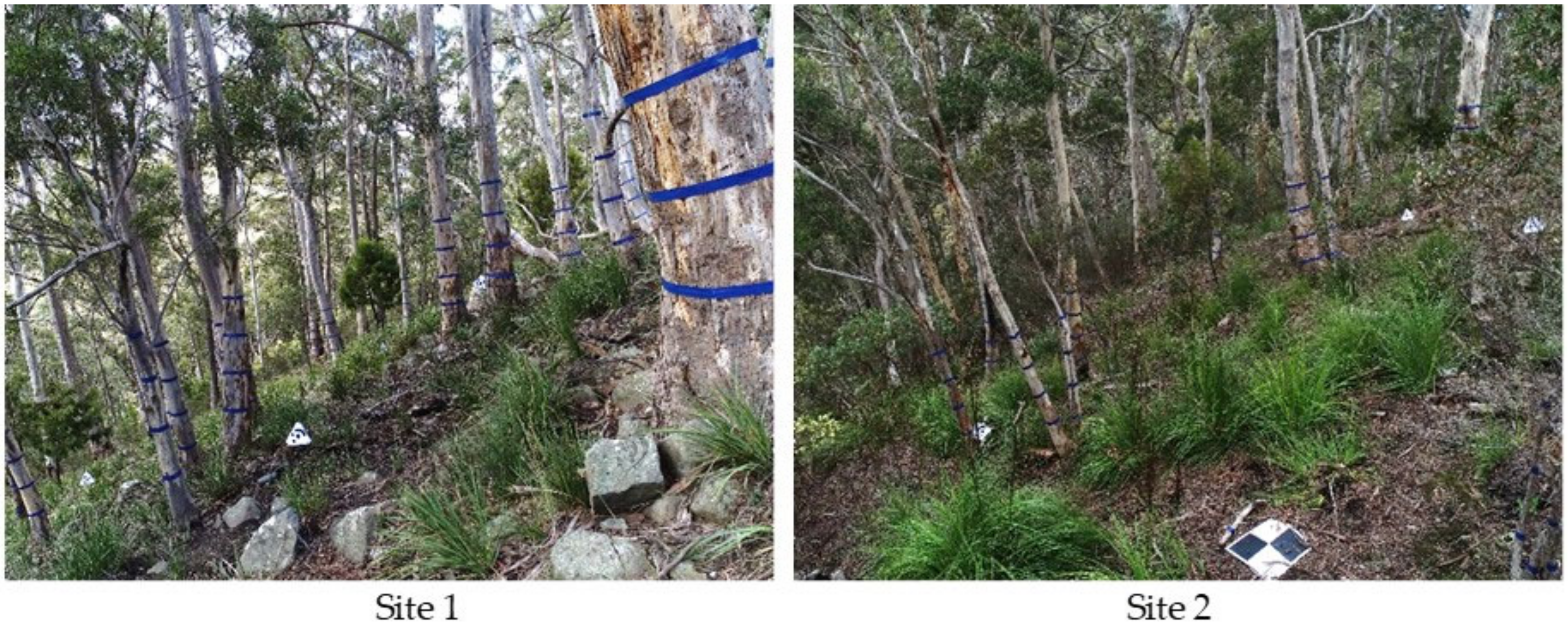
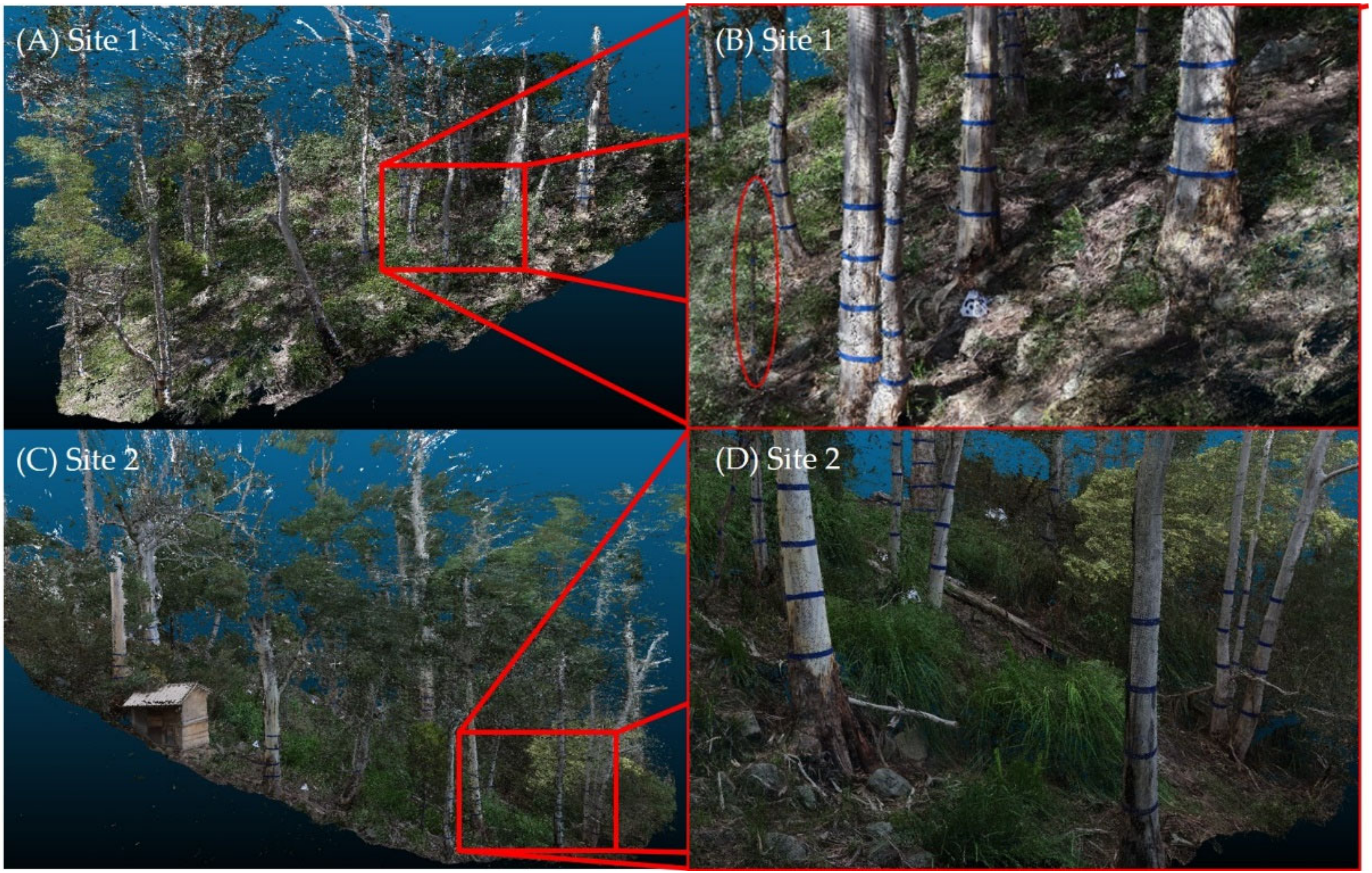
Ground-based techniques including manual field measurement, terrestrial laser scanning (TLS), and terrestrial photogrammetry (TP) are time consuming and thus expensive processes; however, they also pose access and worker safety issues in areas of dense undergrowth. Forest management practices vary considerably around the world; however, rugged terrain and dense undergrowth is common in Australian forest sites where this study was based. 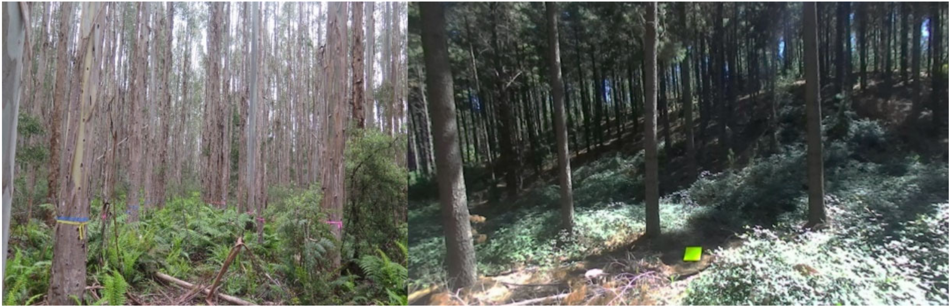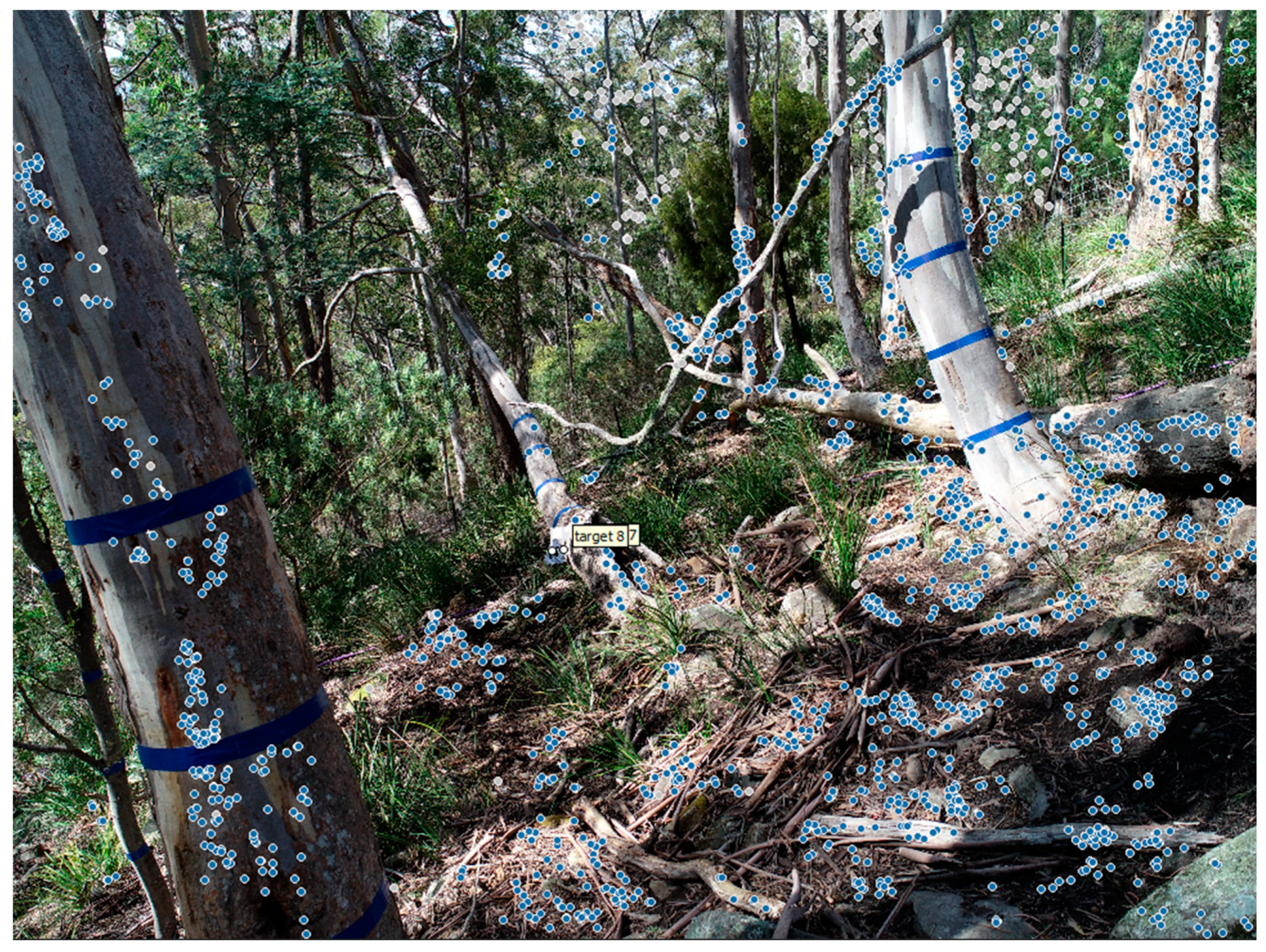Figure 1 shows two examples of the conditions commonly faced in Australian plantation forests. Slips, trips, and falls are among the leading causes of forestry workplace injuries [8,9]. Under-canopy UAS-based remote sensing of forests has the potential to reduce or eliminate forestry workers’ exposure to such safety risks by enabling plot measurements and habitat assessments to be performed from safer locations with less challenging terrain (e.g., at a roadside).

Aside from safety concerns in some areas, manual field measurements and TLS both tend to be relatively slow, costly, and, in the case of TLS, require considerable expertise to implement effectively. While the same can be said about the required expertise to operate UAS currently, UAS-based approaches are well suited to becoming entirely automated. While terrestrial mapping (TLS, TP) can be performed by ground-based robots [10,11], rugged terrain and dense undergrowth can make it more practical to simply fly over the rough terrain. It is easy to envisage such a system where an autonomous ground vehicle (such as a truck) could act as a mobile base station for a fleet of UAS, which can autonomously map areas of forest in unprecedented detail as originally suggested by Jaakkola et al. [12]. To progress towards this vision, it is necessary to explore the efficacy and accuracy of using existing UAS and sensors to map forests beneath the canopy.

There have been few studies so far to explore the use of under-canopy UAS [13,14,15,16,17,18,19]. The existing studies can be grouped into either primarily forest mapping or autonomous navigation-focused studies. Note that while autonomous navigation typically requires mapping to occur, it is necessary to distinguish between navigation-grade maps (for autonomous flight) or forest measurement-grade maps. Such map types have different requirements based on processing time, the type of sensors used, and the power of on-board computing on the UAS. For navigation purposes, granularity is traded off in favor of rapid processing, as map generation is usually needed in real time. Forest measurement-grade maps on the other hand, can have longer processing/optimization times as they are not restricted by real-time map generation requirements or limitations imposed by light-weight on-board computer systems. Thus, they can be of considerably finer granularity than their real-time counterparts.

Four autonomous navigation-focused studies on under-canopy UAS were found in our search [16,17,18,19]. While autonomous navigation will be highly beneficial and possibly even essential for the widespread implementation of under-canopy UAS, our study was not focused on the autonomy aspects; instead, our study focused on the problem of mapping the forest using under-canopy UAS.

The under-canopy UAS studies which focus on mapping include the work by [13,14,15]. The most similar research to ours was performed by Kuželka et al. [13], who tested a Dà-Jiāng Innovations (DJI) Phantom 4 and DJI Mavic Pro for under-canopy AP of a forest in the Czech Republic with Global Navigation Satellite System (GNSS) based scaling of their point clouds.

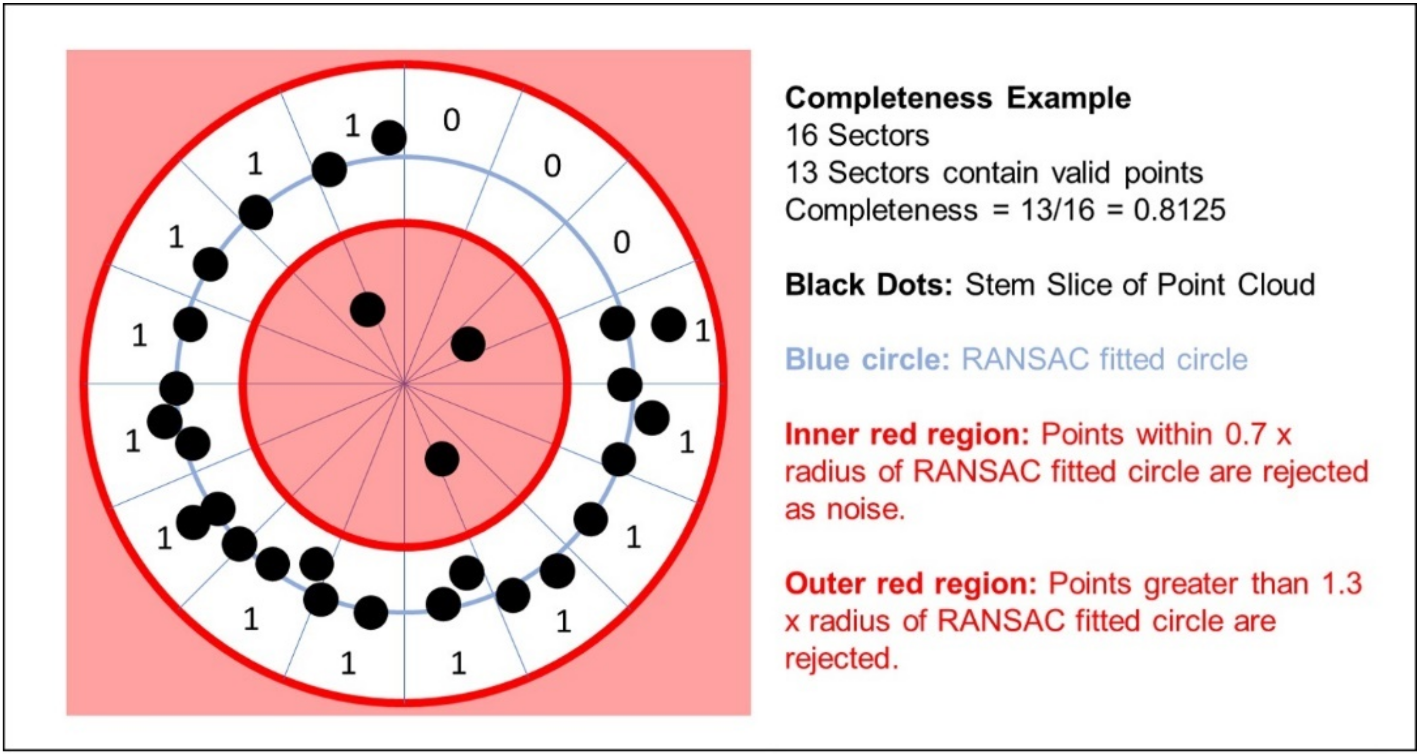
Kuželka et al. [13] also looked at the effect of the number of photos of a stem on the diameter accuracy, which led us to the question: How do we quantify the point cloud coverage in the region of each diameter measurement in any dense point cloud of a forest irrespective of the sensor used? Literature on diameter measurement in forest point clouds was searched to find articles which were quantifying the coverage of points around a stem where a diameter measurement was being taken. Bienert et al. 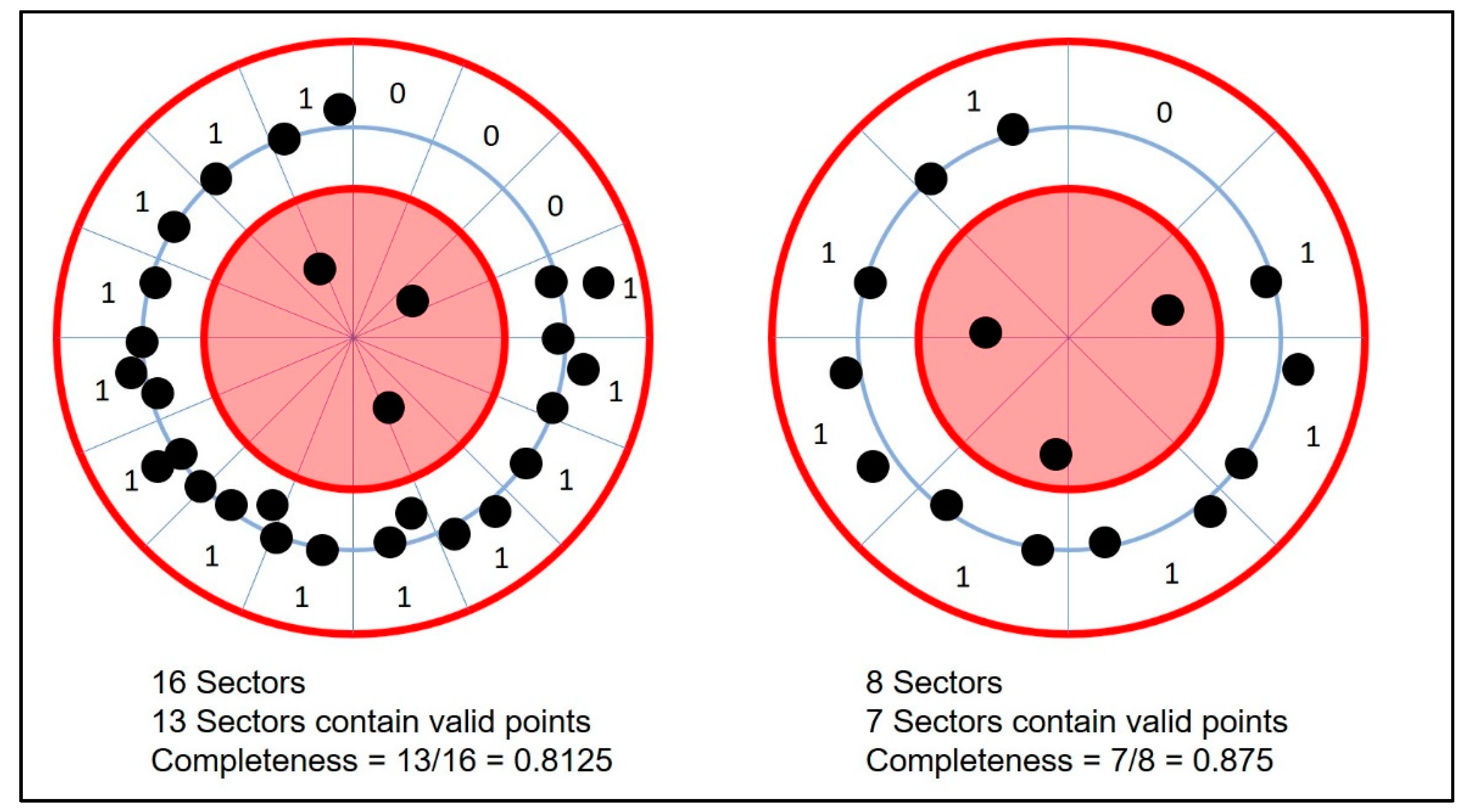[20] introduced a term called “reliability factor”, which was intended to detect over-/under-estimated diameter measurements. As part of their reliability factor, they mention the angle of the visible circle section. However, the measurement of this parameter is not explicitly defined. The term “coverage” was used in [21] in the context of the coverage of points around a stem measurement; however, it was also unclear how this was defined in their study. Quantifying the proportion of a stem represented by points where a measurement is taken is important to understand the coverage of a forest in a given point cloud. Therefore, we proposed a clearly defined term called Circumferential Completeness Index (CCI) with the intention that future forest point cloud research can use a consistent and broadly applicable measure to quantify how thoroughly a section of forest has been mapped. This measure is defined in detail in the methodology and results sections; however, it serves to quantify the proportion of a full circle represented by points in a stem slice. In the case of a single-scan TLS point cloud of a forest, all stems would have a CCI less than 0.5, as slightly less than half of the stems could have been mapped by the sensor. It serves to quantify the difference between trees which were well mapped (such as at the center of a plot) against trees which may have been poorly mapped (such as at the edges of a plot or those which were partially obscured during mapping).

The purpose of this study was to build understanding of the challenges and limitations of using an existing off-the-shelf UAS platform for under-canopy forest mapping in complex forests in order to steer future research towards solutions to these challenges. This study also served as a means of understanding how effective an off-the-shelf UAS can be for this application, providing a baseline from which purpose-built under-canopy forest mapping UAS can improve upon. A detailed methodology is provided to enable replication of this study or use of these techniques, and the CCI measure is explicitly defined to enable comparisons of forest coverage between different high-resolution forest mapping devices.

2. Materials and Methods

2.1. Study Site

This study was undertaken on a property in Fern Tree, Tasmania, Australia, in native regrowth eucalyptus pulchella forest. Figure 2 shows the location of the study site in Tasmania. Two 13 m radius plots were set.

Table 1. Site conditions of the two study sites. Diameter at 150 cm above ground level (D150) was reported as this is the most comparable to diameter at breast height (130 cm above ground) commonly used in similar studies.

Site	Number of Stems	Stem Density (Stems/ha)	Min D150 (m)	Mean D150 (m)	Median D150 (m)	Max D150 (m)	Approx. Slope	Under-Story Description
1	47	885	0.024	0.215	0.224	0.576	24°	Vegetation approx. 0.5 m tall, rocky, some coarse woody debris.
2	52	980	0.030	0.214	0.172	0.618	24°	Vegetation up to 2.5 m tall, coarse woody debris, greater complexity than Site 1.

details the basic plot attributes and Figure 3 shows photos of the conditions of each site.

Both sites were steep with a mean slope of 24°. Large rocks, coarse woody debris, and sudden terrain changes were common. Site 1 had a mostly low understory of approximately 0.5 m tall and had more flyable space than Site 2. Site 2 had understory vegetation of up to 2.5 m tall with multiple unflyable areas and a small shed in the plot area. Vegetation consisted of mostly eucalyptus pulchella trees, with some acacias, tea trees, and banksia trees present.

2.2. Manual Field Measurements

Approximate tree position was measured by taking bearings using a compass (M3 Global, Suunto, Vantaa, Finland) and distance from the plot center using a laser rangefinder (LMR-025, Ozito, Bangholme, Victoria, Australia) fixed to a tripod (MHXPRO-3W, Manfrotto, Cassola, Italy). The stem radius was added to the distance measurement to account for the rangefinder measuring to the nearest side of the tree and not the tree center. These positional measurements were only used to ensure the correct association of field measurements with the point cloud measurements. Figure 4 shows the visualized manual measurements, which were used to correctly label the stem slices from the point clouds with their corresponding reference measurements and notes. Where forks were present (within range of the measurement heights), all stems were measured and taped. Bearings were measured for individual trees and not individual measurements, so a numbering system and field notes were used to ensure correct association of manual measurements with point cloud measurements.

While it remains common practice to measure diameter at breast height (DBH) or 1.3 m above the ground, this is an arbitrary measurement height unless using a model which requires that specific height be measured. This study was not using allometric models, so DBH was not collected. Marking tape was applied to each tree at heights of 0.5 m, 1.0 m, 1.5 m, and 2.0 m above the ground; however, this could be applied to any set of measurement heights, including DBH, if required. These tape marks simply served as a visual reference mark for comparing the manual diameter measurements against those collected using AP. This marking tape was applied perpendicular to the major axis of the stem. Measuring tape was used to measure the stem circumference (later converted to diameter) and was applied around the center of the marking tape, as seen in Figure 5.

This marking tape-based approach is, of course, not recommended for real-world application of under-canopy UAS AP; however, the purpose of this approach was to reduce uncertainty in quantifying diameter measurement accuracy in the point cloud. Digital terrain models (DTMs) are commonly used in remote sensing to measure diameter at a specific height on a stem (such as DBH); however, we chose to avoid the use of a DTM in this study as we were interested in quantifying diameter measurement accuracy without the influence of DTM accuracy. Using a DTM would introduce unnecessary uncertainties to the measurement being quantified due to the difficult-to-define height of ground beneath the tree. Figure 3 (left) illustrates this point in the right of the image, where several large rocks surround the base of a tree. In manual field measurements, such a height would typically be measured from the ground on the uphill side of a tree; however, with the complexities of rocks, sudden terrain changes, and leaning trees, this height becomes difficult to clearly define in a way which can be consistently extracted in a DTM. Automatic point cloud measurement, while critical for the widespread implementation of remotely sensed datasets to forest measurement, was beyond the scope of this article.

Many of the stems throughout both sites were notably noncircular, so each diameter measurement was also labeled with a qualitative note of “circular” or “noncircular”. Any tree with a diameter less than 2 cm at a height of 1.5 m was not recorded.

2.3. Imagery Collection

Images were captured with a DJI Phantom 4 Pro V2 (Dá-Jiāng Innovations Science and Technology Co. Ltd., Shenzhen, China) at a resolution of 4864 × 3648 and frequency of 0.5 Hz in JPEG format. JPEG format was chosen instead of RAW to enable a faster image capture rate (maximum image rate in RAW is 0.2 Hz). The Phantom 4 Pro V2 has a sensor size of 13.2 mm × 8 mm, a focal length of 8.8 mm, and a mechanical shutter [23]. Manual camera settings were used during image capture. Focus was set to infinity and aperture was set to f/2.8 to maximize light input and minimize exposure time and ISO. ISO values were manually controlled between 100 and 400, and exposure time was 1/500 s. The tests were performed around midday in spring with the sun to the north. It was mostly sunny, however, there was patchy cloud cover changing the light conditions throughout the flight and requiring adjustments to ISO during the flight. Image capture began once eight satellites were being used for global position in the slightly clearer take-off area.

2.4. Coded Targets

Informal experimentation by the authors prior to this study found that placing coded targets in the field greatly aided the reliability of the image alignment process. Coded targets should be attached to flat surfaces [24] and, for this application, needed to be quick to deploy in the field. To achieve this, truncated tetrahedron-shaped targets were made from 5 mm thick foam board with a 12-bit coded circular target on the three upright faces. The underside face of this tetrahedron was omitted to allow stacking of these markers for ease of deployment and transport. The outermost diameter of the circular targets was 0.17 m. Ten of these tetrahedrons were placed throughout each plot, providing a total of 30 coded targets in each plot. An example of these targets can be seen in Figure 6. A 0.9 × 0.9 m, square, black-and-white checkered target was also placed in the field to denote the plot center (seen in Figure 3, Right). Distance between these coded targets was not manually recorded, as these targets were not used as ground control points and were only used to assist the alignment process by providing high-confidence point matches to Agisoft Metashape (www.agisoft.com). These coded targets met the criterion of being quick to deploy in the field, taking approximately 5 min to deploy in each site. Locations of these markers are visualized in Figure A1 in the Appendix.

2.5. Under-Canopy Flight Strategy

The UAS was manually piloted by visual line of sight using DJI’s “Tripod” flight mode. Tripod mode limits flight speed to 7 kph and reduces the sensitivity of the controls to assist the pilot to keep movements slow and precise [25]. Actual flight speed was kept to approximately 0.5 m/s to minimize motion blur and to ensure high overlap of the imagery. Due to the complex 3D nature of close-range photogrammetry (as opposed to above-canopy nadir photogrammetry with a grid pattern), image overlap is not easily defined and, without automation, is nearly impossible for a pilot to control precisely. This system lacked any mapping feedback other than the camera view on a tablet display which assists the pilot to aim the camera. Vision positioning was enabled, as this assisted the pilot in making gentle and precise movements with minimal position drift due to disturbances such as a light breeze. Robust position holding is useful to prevent the aircraft drifting into nearby obstacles.

The DJI Phantom 4 Pro V2 aircraft is capable of basic collision avoidance via three stereo cameras and ultrasonic and infra-red rangefinders [23]. However, this collision avoidance system hindered the effective use of this aircraft below the canopy and was disabled for this study. If the collision avoidance system included an adjustable collision box, collision avoidance would have been highly beneficial and would reduce the mental load on the pilot. With collision avoidance switched off, there was full reliance on the pilot to not collide with the many obstacles present.

Path planning for repeatable and reliable data capture under the forest canopy is a challenging problem when stems are not in neat rows such as in intensively managed forests. The flight strategy was to capture images of all sides of the trees within the plot, while attempting to see the coded targets within as many images as possible. The camera was aimed at approximately 30 degrees below horizontal with flying height above ground varying from 3 m to 20 m depending on the unoccupied space available to fly in. There were unflyable regions in both plots, and this was reflected in the flight paths. Both flights were of 20 min’ duration and captured approximately 600 images per flight.

2.6. Photogrammetric Processing

Agisoft Metashape Professional [26] was used for the photogrammetric processing in this study. Point cloud-scale was provided by onboard geotagging of the images and was additionally constrained by the camera alignment process in Metashape.

Table 2. The settings we used in Agisoft Metashape in this study. For details on these settings, please consult the Agisoft Metashape Manual [24].

Stage	Settings	Value
Estimate Photo Quality	Remove images with quality < 0.7	-
Detect Markers	Tolerance	100
Align Photos	Accuracy	Highest
	No. Keypoints	20,000
	Max. No. Tiepoints	4000
	Generic Preselection	Off
	Reference Preselection	Source
	Adaptive Camera Model Fitting	No
Optimize Cameras	-	-
Build Dense Cloud	Quality	High
	Depth Filtering	None
Export Points	Output File	.las

details the settings and processes used in the reconstruction. Some images were initially misaligned and required correction by resetting camera position, manually tagging any unidentified coded targets in the images, and re-running the alignment process. The camera was not precalibrated.

The generated point clouds contained approximately 230 million points each and can be seen in Figure 7. The level of detail achievable with the photogrammetric process was constrained by the resolution and clarity of the images used. In conventional AP applications, a term known as ground sample distance (GSD) is used. GSD is the size of a pixel at ground level. In the case of this work, the imagery was collected at oblique angles rather than at nadir; however, the concept of pixel size at a projected location is still useful. Since we are not only referring to ground samples, we will instead call this measure target sample distance (TSD) to minimize confusion. Plots in this study were of 13 m radius, so at a full 26 m range from one side of the plot to an object at the boundary on the other side, the TSD would be 15.6 mm. At the closest object proximity to the camera of approximately 1 m, the TSD would be 0.6 mm. With sub-centimeter GSD values, it was possible to reconstruct fine details down to individual blades of grass, as seen in Figure 7D. It should be noted that if such levels of details are sought, the objects must remain completely still during the image capture process, otherwise they will not be reconstructed correctly, if at all. Fine details can be traded off in favor of faster processing time by setting the dense cloud quality to medium.

2.7. Point Cloud Post-Processing

To ensure that measurements of diameter from the point cloud were taken at the same position as the manually collected measurements, a section of the stem marked by blue tape was manually sliced from the point cloud using CloudCompare (http://www.danielgm.net/cc/ [27]). In the cases of small stems where the blue taped section was poorly reconstructed, these were not used further and were noted as missing point cloud measurements. Points which were not to be used in measurements (such as branches or neighboring vegetation) were manually removed, and the remaining points were labeled to correspond with the manual diameter measurements. A custom computer program (written in Python 3.6) first fitted a plane to each of the stem slices using singular value decomposition. This plane provided the necessary information to rotate the slice of points to a horizontal orientation to allow the application of random sample consensus (RANSAC)-based 2D circle fitting [13]. After measuring diameter and CCI in 2D, the fitted circle was rotated back to the original orientation for visual confirmation that the data processing worked as expected. Such a visualization is shown in Figure 8. An enhanced version of the custom software used in this study will eventually be made available as part of an automated point-cloud post-processing tool currently under development.

This article presents a new measure for forest point clouds called Circumferential Completeness Index (CCI). This is defined as the fraction of a full stem circle represented by points. A simple visualization showing how this can be calculated is shown in Figure 9. The points of the stem circle/arc are divided up into angular regions with respect to the center of the fitted circle and co-planar with the fitted circle. Each region is checked for the presence of points and, if points are detected within an angular region and are greater than 0.7 × the fitted circle radius, that region of the stem is considered to be “complete”. The cutoff value of 0.7 × the radius was used in order to ignore noise points which may exist inside the fitted circle and would affect the accuracy of the CCI. It is also suggested to have an upper cutoff value of 1.3 × the radius if the stem slice used contains branching, noise points, or nearby stems. The cutoff values, like the number of angular regions, can be adjusted as required for individual datasets with minimal impact upon the CCI value.

If all angular regions of the circle contain points, the CCI is 1. If only half of the arcs contain points (such as for a tree only viewed from one side), the completeness would be 0.5. Use of this completeness score metric does require consideration of the point density and is primarily intended for use with very high-resolution point clouds such as those created using TLS, high-resolution ALS, or close-range photogrammetry. It is possible to use this measure with lower resolutions than those achieved in this study provided that a clearly defined stem circle can be extracted. Choice of angular divisions (5 degrees in this study) will need to match the data it is applied to; however, this will only affect the precision of completeness index and not necessarily the consistency of the measure. This is visualized in Figure A2.

When reporting the mean CCI for a point cloud, it is suggested to specify whether the mean CCI includes missing measurements or excludes them. It is possible to include the missing measurements provided that you have collected data on the exact number of stems/measurements in the field site and know how many missing measurements there are. In the primary use case of only collecting a point cloud, the number of missing measurements is likely unknown. We suggest that mean CCI is, therefore, reported as “validated mean CCI” (missed measurements are known) or “unvalidated mean CCI” (missed measurements are unknown). If validated mean CCI is reported, it is suggested to also report unvalidated CCI to enable comparisons to be made with point cloud-only studies.

3. Results

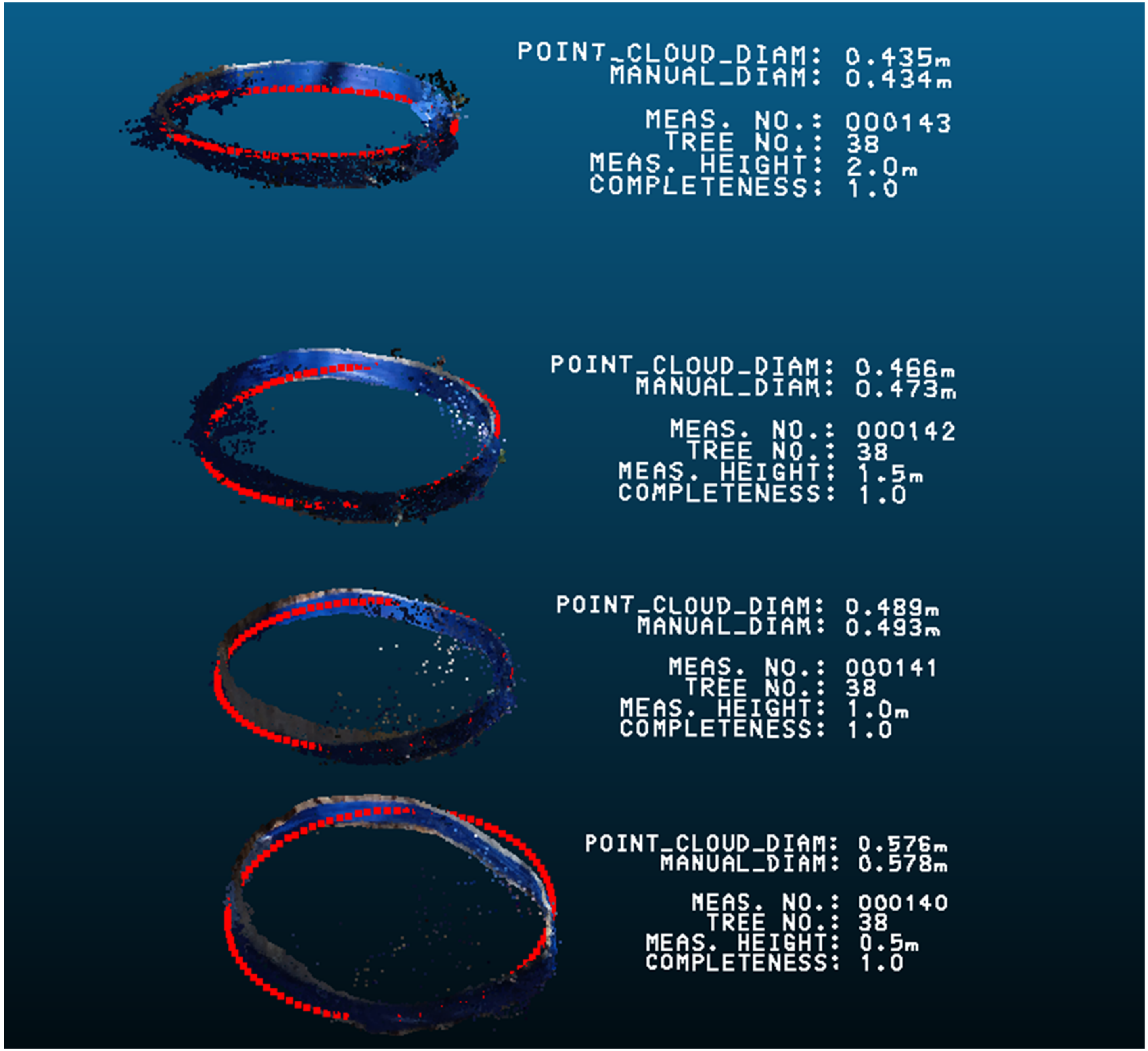
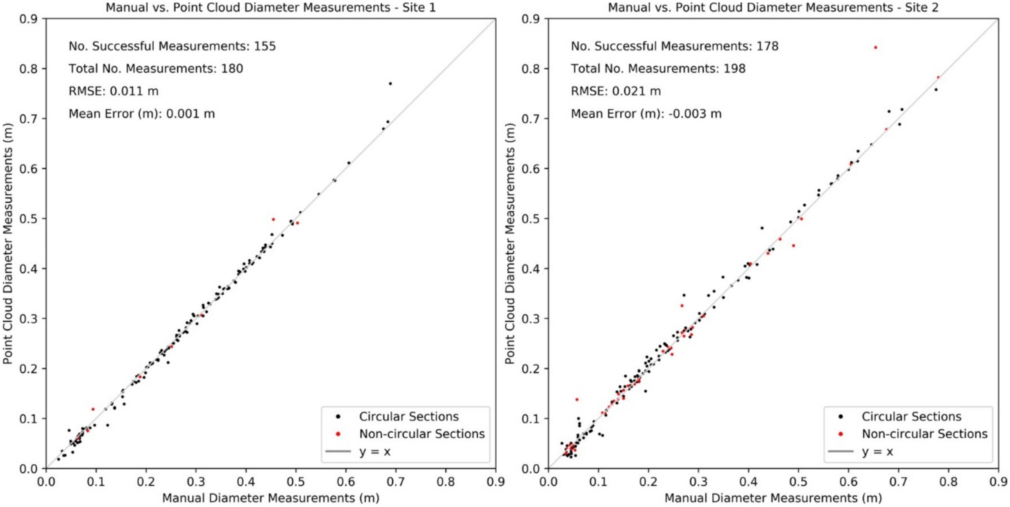
In the Site 1 point cloud, 155 out of 180 taped diameter measurements were successfully detected in the point cloud. In the Site 2 point cloud, 178 out of 198 taped diameter measurements were successfully detected. In total, 333 out of 378 taped sections were detected, giving a detection rate of 88% at the individual measurement level. At the individual tree level, all measured trees within the two sites were visually identifiable in the point cloud; however, measurements were not able to be taken from all stems due to the absence of a clear stem circle in the point cloud. There were two trees where none of the four diameter measurements could be taken, one in each site. In Site 1, the unmeasurable tree had a diameter of 4.8 cm at 1.5 m height, and at Site 2, the unmeasurable tree had a diameter of 5.4 cm at 1.5 m height. If we consider a stem to be “detected”, if it has at least one measurable stem circle at a taped section, there was a 97.8% tree level detection rate in Site 1 and a 98.0% tree level detection rate in Site 2.

The root-mean-squared errors (RMSE) of the successful diameter measurements were 11 mm and 21 mm for Sites 1 and 2, respectively. Site 1 had a mean diameter error of +1 mm and Site 2 had a mean diameter error of −3 mm. These results are visualized as scatterplots of manual tape-based measurements of diameter versus the point cloud-based measurements of diameter in Figure 10.

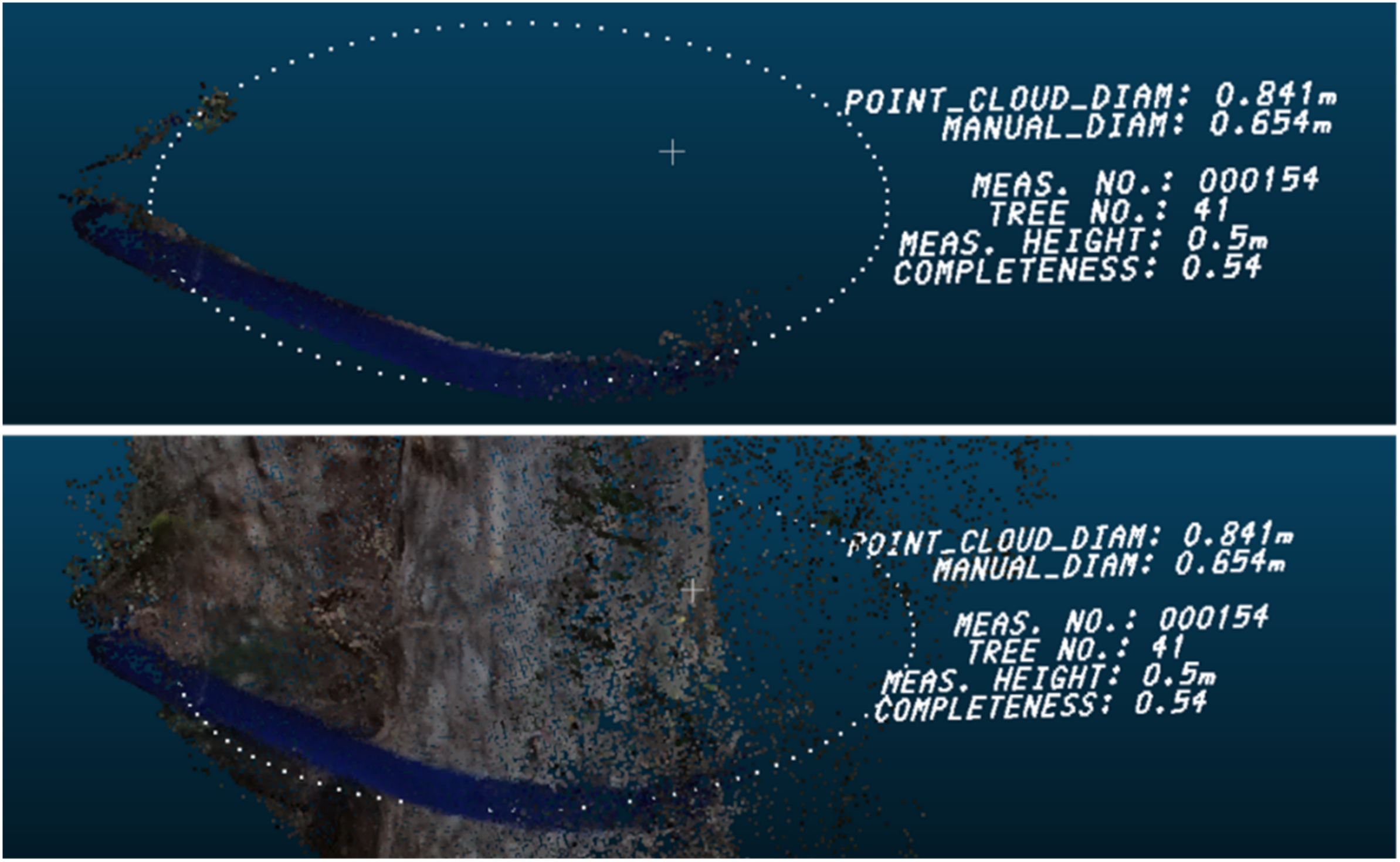
In Site 1, nine of the 180 diameter measurements were noted as noncircular. In Site 2, 40 out of the 198 diameter measurements were noted as noncircular. An example of a noncircular stem from Site 2 is shown in Figure 11, where a tree was forked near ground level resulting in a peanut-shaped cross-section. The point cloud-based diameter measurement was 0.841 m at 0.5 m height, compared to the measuring tape-based manual diameter measurement of 0.654 m. It is also worth noting the CCI of the stem. Even though the circle was a sub-optimal model for fitting due to the noncircular shape of the stem, the CCI was still reasonable for the cross-section, suggesting that 54% of the stem circumference had been mapped at that cross-section.

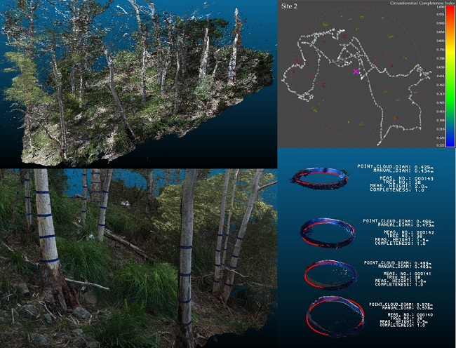
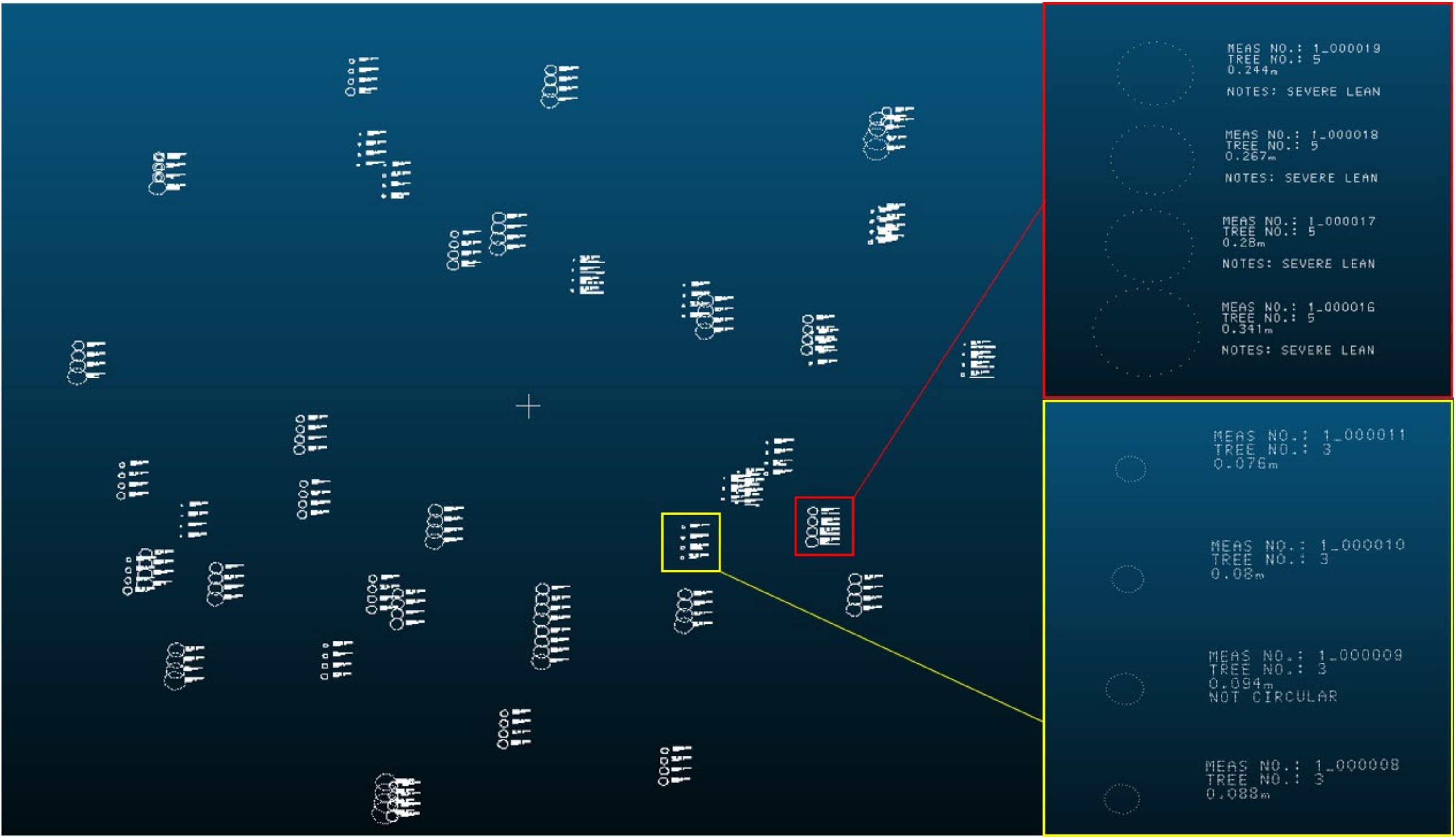
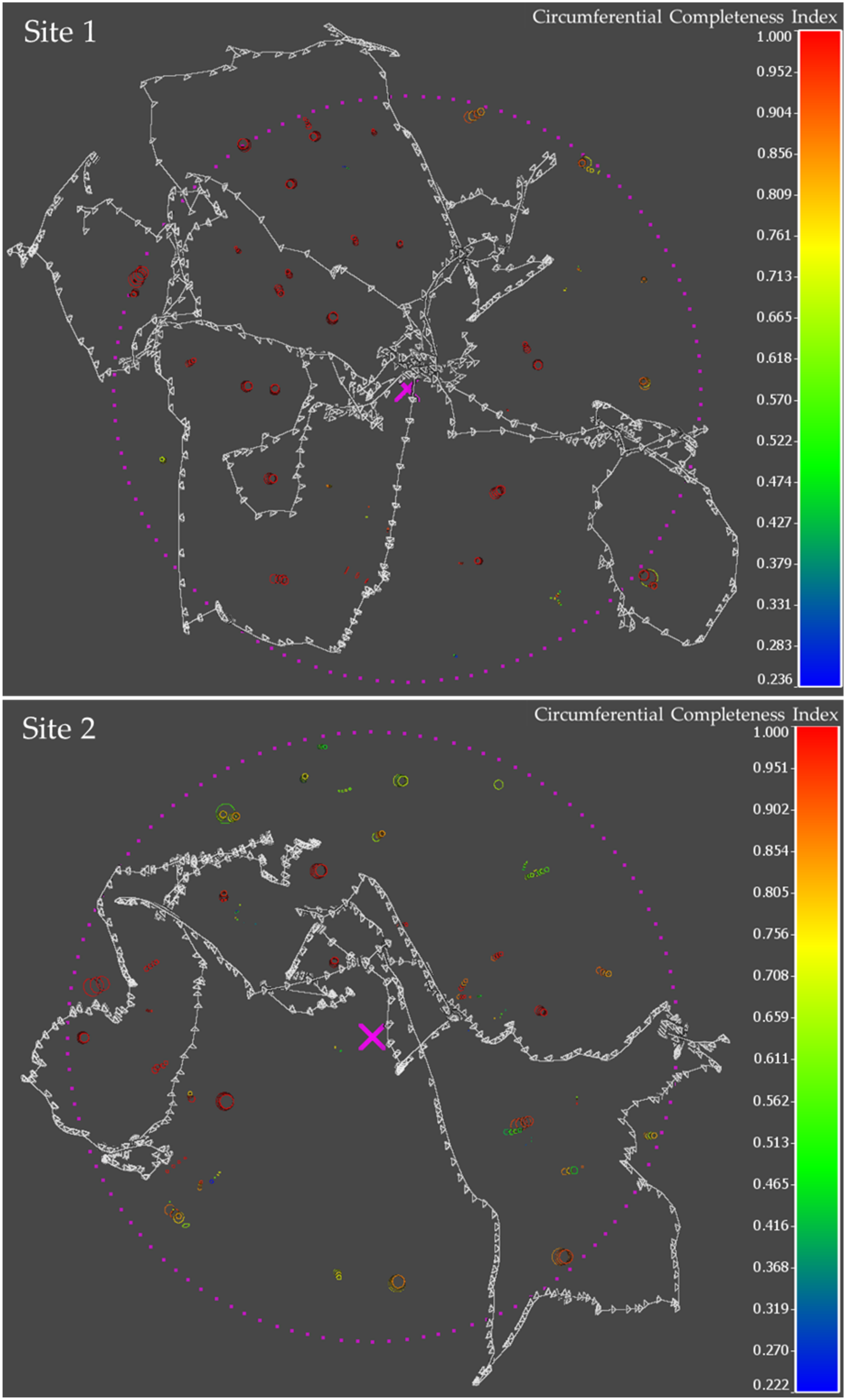
In Figure 12, CCI is visualized in the context of stem locations and the flight paths/camera orientations. The stems were visualized by RANSAC fitted circles, colored by the CCI of each diameter measurement. The CCI was high for stems seen by many photos and low in areas with fewer photos, as expected. It is important to note that there were areas in both Sites 1 and 2 which were unflyable due to the presence of dense vegetation. Stems within these areas had a lower CCI as they could not be seen from all angles and were imaged from further away.

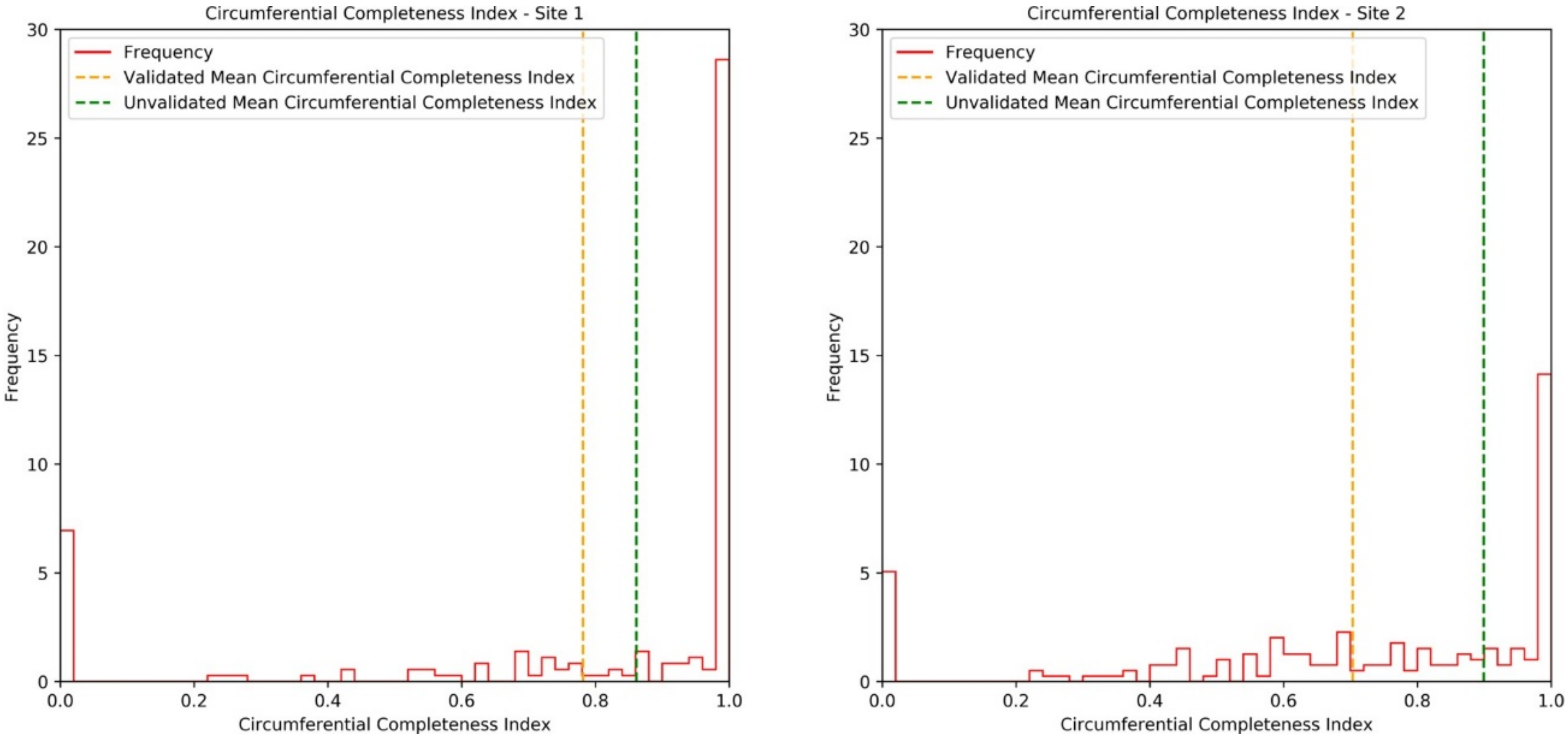
The validated mean CCI values were 0.78 for Site 1 and 0.70 for Site 2. The validated and unvalidated median CCI values for Site 1 were 1.0, meaning that greater than half of the point cloud measurements taken had complete circles of points around the tree. The validated median CCI for Site 2 was 0.78 and the unvalidated median CCI was 1.0. Histograms are shown for both sites in Figure 13 to visualize the distribution of CCI under the differing site conditions. A well-mapped section of forest would be skewed to the right in these plots and a poorly mapped region would be skewed to the left. It was expected that Site 2 would be less complete overall due to the dense understory and reduced flyable space, making the mapping process more difficult than in Site 1.

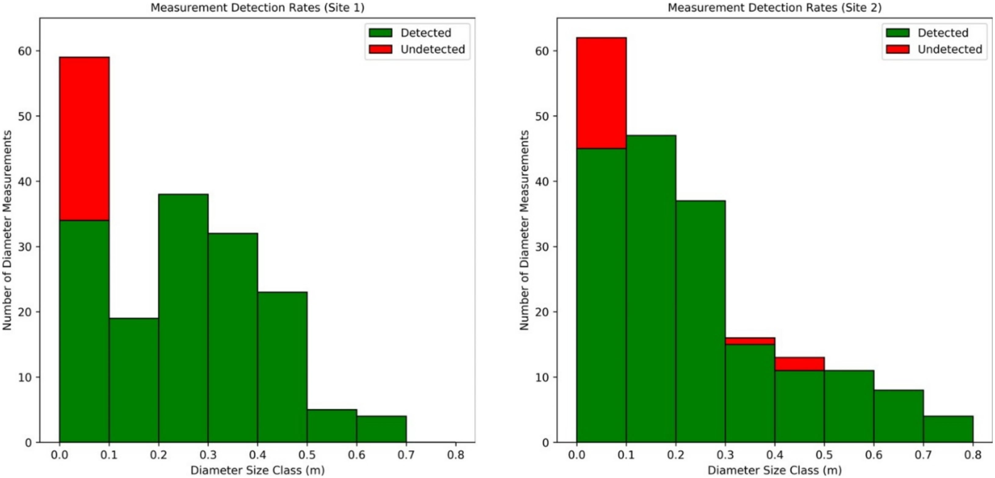
As a result of the dense understory in parts of Site 2, some larger measurements were obscured by vegetation and were not reconstructed. In both sites, the majority of undetected measurements were in the 0.0–0.1-m-diameter size class. This is shown in Figure 14.

4. Discussion

Prior under-canopy UAS-based studies achieved root-mean-squared errors of diameter measurements (relative to manual measurements) of 41 mm with AP [15] and 78 mm with 2D Light Detection and Ranging (LiDAR) [14]. The most comparable study to ours was performed by Kuželka et al. [13]. They tested their approach on two 50 × 50 m-square plots, with stem densities of 290 and 270 for each respective plot. Their study was performed in sites with no understory and generally flat topography. Our study differed considerably with respect to forest conditions, with a diverse mix of tree species, a complex understory, rocks and boulders, and rough, steep (24° average slope) terrain. They obtained RMSEs (relative to field measurements) of 48.7 mm for point cloud-based diameter measurements using least squares circle fitting (the most comparable diameter measurements to our method).

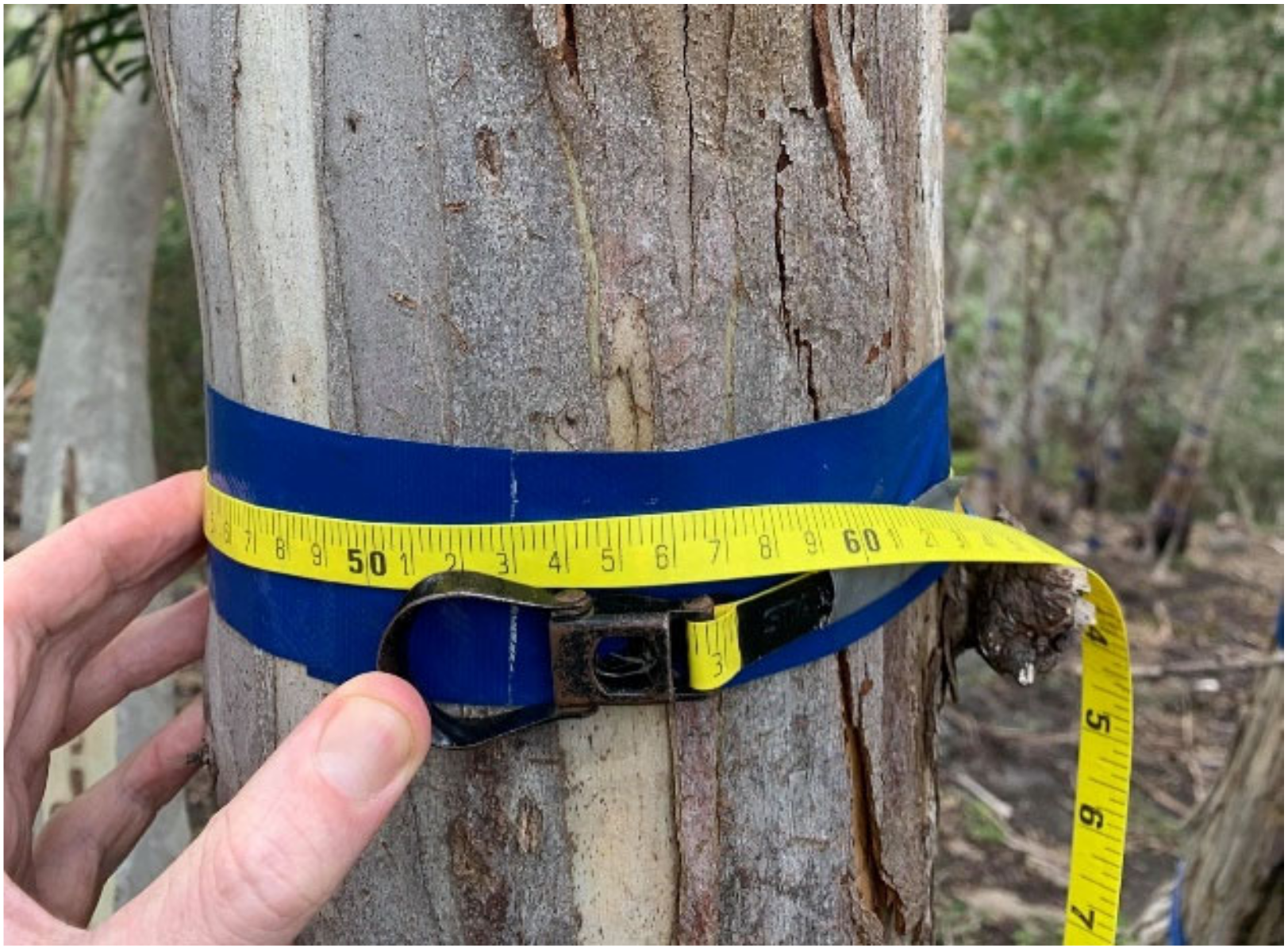
It is also interesting to compare these results to other remote sensing techniques such as TLS and TP. Piermattei et al. [28] used a tripod-mounted Digital Single Lens Reflex (DSLR) camera and compared their TP point clouds against TLS point clouds and caliper-based reference measurements as a baseline. They reported RMSEs for diameter at breast height (DBH) measurements of 12.1 mm, 20.7 mm, 50.7 mm, and 40.2 mm for TP measurements and RMSE values of 8.7 mm, 37.5 mm, 13.8 mm, and 11.3 mm for TLS vs. caliper reference measurements. We measured RMSEs of 11 mm and 21 mm in Site 1 and Site 2, respectively, relative to tape-based diameter measurements. Based on these results, our approach was comparable to both TP and TLS at measuring diameter and was notably more accurate than the prior under-canopy UAS studies, including one using a similar UAS platform. The reason for such accuracy in our study was likely due to the use of the tape-marked measurements effectively eliminating the additional errors caused by comparing manually measured heights above ground against DTM-based heights above ground. In this study it was possible to confidently measure diameter at the same position on the tree as when measured manually without relying on a DTM for height above ground due to the blue tape marks. This may play an important role in quantifying the RMSE of diameter measurements, as the research team minimized the error in the measurement height that would influence the error in the diameter measurement. In simple terrain with gradual changes in slope, the DTM-based measurement height may align well with field-based measurement height; however, in the study sites chosen for this work, it was challenging to define a rule (even in the manual field measurements) which would work consistently for all cases in the sites due to rocks and frequent, sharp changes in local slope. Measurement accuracy, while important, is not the only necessary consideration when choosing remote sensing technologies for an application. Practicality, time cost, sensor cost, and completeness of the data contribute to how useful a given approach is.

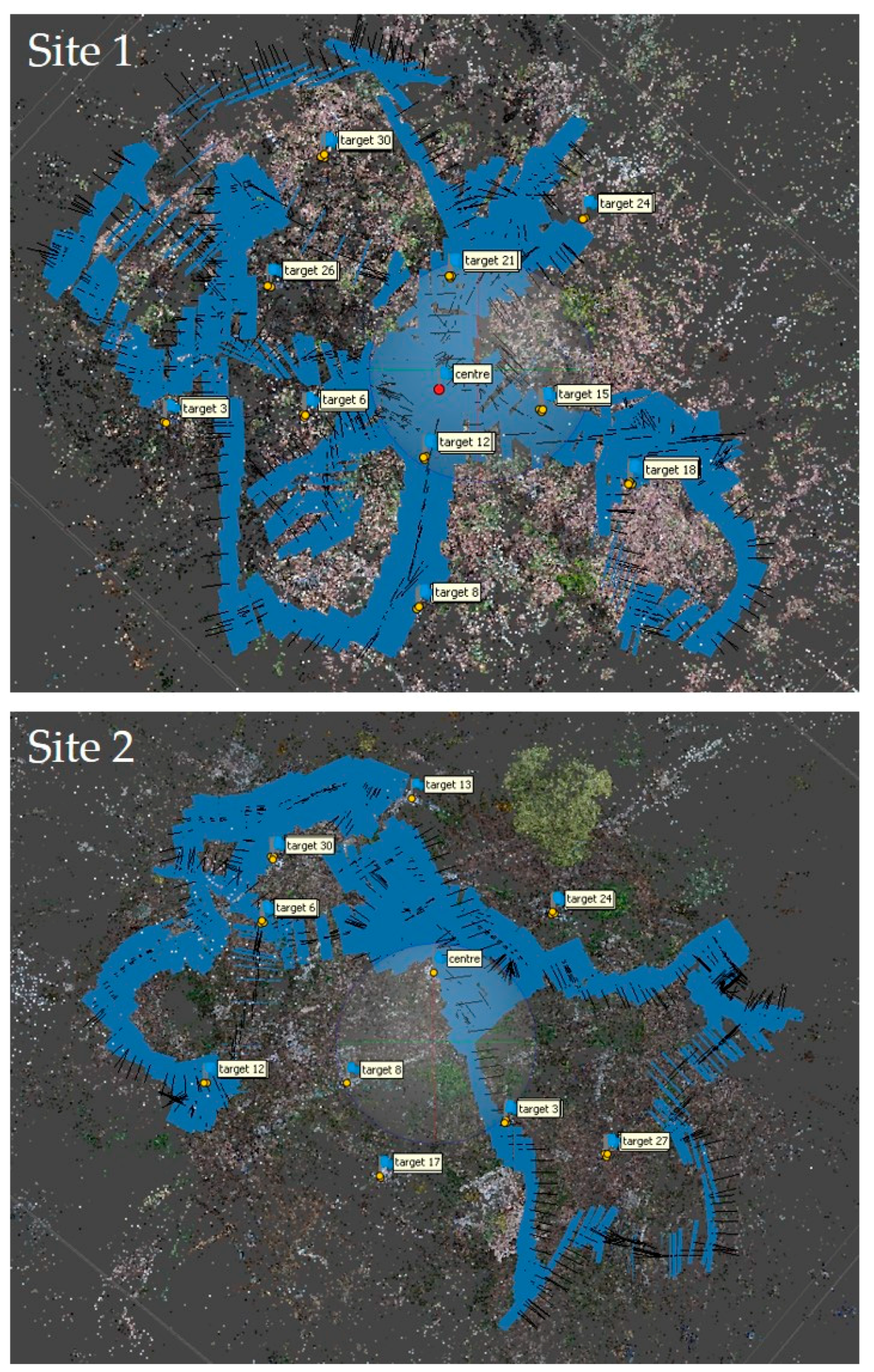
From a practicality standpoint, the test conditions of our study involved a dense understory, high stem density, and a steep slope, and our UAS-based methodology was highly effective in minimizing the need to traverse this terrain. While coded targets were placed in the field to help with the image alignment process, they were able to be placed in the most easily accessible parts of the sites (which conveniently also tend to be the most visible regions for such a target to be placed), allowing the operator to avoid traversal of the most difficult terrain. It should be noted that even with the placement and retrieval of these targets, there is considerably less terrain traversal required compared to TP. To appreciate the reduction in terrain traversal despite the placement of targets, we could consider the acquisition time of up to 2 h for similar plot sizes with TP in [28], against the 5–10 min per plot to place and retrieve the coded targets in our study. The use of such coded targets should be considered a short-term work-around until photogrammetry or similar remote sensing techniques can work reliably in these conditions without such targets.

The reliance upon GNSS for scaling of under-canopy AP point clouds is not going to work in all forest situations. GNSS was highly effective for providing scale under the tested conditions as well as the test conditions in [13]. HHowever, GNSS signal is commonly degraded or entirely absent under dense forest conditions [29]. In the short term, ground control points with known distances or scaled targets will need to be used in sites with insufficient GNSS reception. For scaling of photogrammetric point clouds, stereo cameras and visual inertial systems show promise in this area and may offer low-cost solutions to this problem in the near future.

In terms of time cost, our image capture process required 20 min per flight with an additional 5–10 min to place and retrieve the coded targets. Photogrammetric processing of the data was mostly automated in Agisoft Metashape (some minor image alignment corrections were required). Our post-processing of the point cloud was time consuming due to the manual trimming of the tape circles; however, this would not be performed outside of this study, as this was only used for the purposes of measuring the accuracy of diameter measurement without the influence of a DTM. Instead, it is suggested to perform post-processing of the point cloud with partially automated tools, such as 3D Forest [30] or Computree [31], until fully automated and reliable tools become available.

In terms of sensor cost, a DJI Phantom 4 costs $2400 Australian Dollars (AUD) at the time of writing, comparable to a decent DSLR camera and lens. A TLS system can be well upwards of $30,000 AUD, although exact pricing is seldom advertised online.

In terms of completeness of the data, we suggest that Circumferential Completeness Index (CCI) be reported as a standard measure in future research using diameter measurements of forest point clouds such that the overall coverage of a study site, as well as coverage of individual stems, can be better communicated among the scientific community. The sites studied in this work had validated mean CCI of 0.78 and 0.7 and unvalidated mean CCI of 0.86 and 0.89 for Sites 1 and 2, respectively. Future work which uses CCI is expected to mostly report the unvalidated mean CCI, as this only requires a point cloud and does not require manual field measurements. We suggest that alongside the unvalidated CCI, the most meaningful way to communicate this measure is to provide a histogram to show the distribution of CCIs for the successful diameter measurements, as shown in Figure 14.

A limitation of CCI is that it is context dependent and there are stem shapes which will not provide a meaningful CCI value. It is based on the fitting of a circle to the stem and so may not work reliably for highly noncircular stems, such as the example shown in Figure 12. In this case, a stem with a peanut-shaped cross-section resulted in a poor circle fit and this would have had an impact upon the measurement of completeness. With that said, the CCI in this example still appears reasonable for the stem considering the proportion of stem captured. A circle was used in this study to find the stem center; however, future work may explore the use of a noise-tolerant convex hull-based approach which could use the centroid of these shapes as the stem center from which to measure CCI. Both circle fitting and the suggested convex hull (such as in [32]) -based completeness metrics would fail to accurately represent a stem if the stem is ‘C’ shaped (such as a partially burnt and hollow stem). ‘C’-shaped stems are indistinguishable from incompletely mapped stems unless the wall thickness of the ‘C’ section is thicker than the noise/error in the remote sensing method used as well as the inside of the ‘C’ being well mapped.

A limitation of the methodology used in this study is that manual trimming of the point cloud was required, introducing some subjectivity to the dataset. While the utmost care was taken to not influence the results, there was some subjectivity in the manual point cloud slicing process, which must be acknowledged. It is possible that additional small stems, which were marked as missing measurements, were successfully reconstructed and were removed/missed in this manual process. This slight subjectivity of manual slicing is expected to have had a nearly negligible effect on large and well-reconstructed stems; however, it would have likely had a negative impact on the small and highly vegetated stems, particularly where some discretion was required when identifying the blue tape in low light and low contrast situations. Wherever there was doubt about tape detection or where there was no clear stem circle/arc from a taped section, the points were considered to be missing measurements and were removed. An additional limitation of this study is that the presence of the blue tape marks throughout the site contributed to some tie points in the image alignment process. This effect appears to have been minimal, as the natural environment provided plenty of unique features used in the alignment process (seen in Figure A3). However, it is necessary to acknowledge that this may have improved the diameter accuracy through better reconstruction in taped regions.

Future research in this area would greatly benefit from improved collision avoidance systems and/or reliable GNSS denied autonomous flight. For systems like the DJI Phantom 4, it would have been particularly useful if a smaller threshold distance/collision box could be specified for taking avoidance action to enable the use of collision avoidance in sites such as those in this study. The large collision box required that collision avoidance be completely deactivated in this study so that the UAS could fly between narrow (yet still safely passable) gaps. Systems such as the Skydio 2 [33] and companies such as Katam Technologies [34] look particularly interesting for addressing some of these autonomy challenges.

Lastly, an operational challenge of under-canopy UAS mapping with an aircraft such as the Phantom 4 is that of path planning for complete data capture. The Phantom only has a single camera (not including the three stereo cameras used for collision avoidance), presenting a challenging optimization problem for a human pilot with no feedback regarding which areas have been sufficiently imaged for successful and accurate image alignment and reconstruction. The optimal path planning problem is particularly difficult to explore through manual flight, as it is challenging to define and follow a structured flight path in a highly unstructured environment. Such an optimization task would be better suited for a machine to compute during flight than a human. Initial attempts were made by the authors prior to this study to explore different flight paths through manual flight; however, it was clear that fully autonomous navigation with repeatable path planning/following is required to explore this problem appropriately as it is difficult for a human to perform repeatable flight patterns/strategies in unstructured forests.

Despite the challenges and limitations of using a consumer-grade, off-the-shelf UAS for under-canopy AP, this approach was still highly effective in both time cost and quality of results. If this was combined with automated point-cloud post-processing, this method may already be faster than measuring a plot with traditional field techniques. In addition to potential time savings, the under-canopy UAS-based approach provides a much richer dataset than field measurements, with the possibility of enabling us to move away from allometric equations and DBH measurements and instead measure volume at the individual stem and branch level, transforming how we measure forests in the future. It is foreseeable that such rich datasets could eventually be incorporated into fully autonomous forest operations from planting and weeding through to harvest [35].

5. Conclusions

This study demonstrated the use of an off-the-shelf DJI Phantom 4 Unmanned Aerial System (UAS) for under-canopy photogrammetric mapping of forests as an effective alternative to manual field plots, terrestrial photogrammetry, and terrestrial laser scanning. This approach was particularly effective considering the structural complexity of the forest and the steep/rough terrain of the study sites. Two sites were measured both manually and with under-canopy UAS photogrammetry and were compared at an individual diameter measurement level at four heights per stem. The point cloud-based diameter measurements had root-mean-squared errors with respect to manual reference diameters of 11 mm and 21 mm for Site 1 and Site 2, respectively. A metric called Circumferential Completeness Index (CCI) was defined for quantifying the coverage of a forest point cloud based on the proportion of a stem circle represented by points in a point cloud slice of a stem. Two variants of this metric were defined: The validated mean CCI and unvalidated mean CCI. Site 1 and Site 2 had a validated mean CCI of 0.78 and 0.70 and unvalidated mean CCI of 0.86 for Site 1 and 0.89 for Site 2.

Future research will focus on the development of a purpose-built under-canopy mapping UAS to address the limitations of the DJI Phantom 4 platform for this application, and a fully automated point cloud post-processing workflow will be developed to bring under-canopy UAS mapping to a level suitable for use in the forestry industry and conservation projects.

References

1. Pádua, L.; Vanko, J.; Hruška, J.; Adão, T.; Sousa, J.J.; Peres, E.; Morais, R. UAS, sensors, and data processing in agroforestry: A review towards practical applications. Int. J. Remote Sens. 2017, 38, 2349–2391. [Google Scholar] [CrossRef]
2. Singh, K.K.; Frazier, A.E. A meta-analysis and review of unmanned aircraft system (UAS) imagery for terrestrial applications. Int. J. Remote Sens. 2018, 39, 5078–5098. [Google Scholar] [CrossRef]
3. Wallace, L.; Lucieer, A.; Malenovský, Z.; Turner, D.; Vopěnka, P. Assessment of Forest Structure Using Two UAV Techniques: A Comparison of Airborne Laser Scanning and Structure from Motion (SfM) Point Clouds. Forests 2016, 7, 62. [Google Scholar] [CrossRef] [Green Version]
4. Wieser, M.; Mandlburger, G.; Hollaus, M.; Otepka, J.; Glira, P.; Pfeifer, N. A Case Study of UAS Borne Laser Scanning for Measurement of Tree Stem Diameter. Remote Sens. 2017, 9, 1154. [Google Scholar] [CrossRef] [Green Version]
5. Lisein, J.; Pierrot-Deseilligny, M.; Bonnet, S.; Lejeune, P. A Photogrammetric Workflow for the Creation of a Forest Canopy Height Model from Small Unmanned Aerial System Imagery. Forests 2013, 4, 922. [Google Scholar] [CrossRef] [Green Version]
6. Hollaus, M.; Wagner, W.; Eberhöfer, C.; Karel, W. Accuracy of large-scale canopy heights derived from LiDAR data under operational constraints in a complex alpine environment. Isprs J. Photogramm. Remote Sens. 2006, 60, 323–338. [Google Scholar] [CrossRef]
7. Næsset, E. Practical large-scale forest stand inventory using a small-footprint airborne scanning laser. Scand. J. For. Res. 2004, 19, 164–179. [Google Scholar] [CrossRef]
8. Tsioras, P.A.; Rottensteiner, C.; Stampfer, K. Wood harvesting accidents in the Austrian State Forest Enterprise 2000–2009. Saf. Sci. 2014, 62, 400–408. [Google Scholar] [CrossRef]
9. Bentley, T.A.; Parker, R.J.; Ashby, L.; Moore, D.J.; Tappin, D.C. The role of the New Zealand forest industry injury surveillance system in a strategic Ergonomics, Safety and Health Research Programme. Appl. Ergon. 2002, 33, 395–403. [Google Scholar] [CrossRef]
10. Pierzchała, M.; Giguère, P.; Astrup, R. Mapping forests using an unmanned ground vehicle with 3D LiDAR and graph-SLAM. Comput. Electron. Agric. 2018, 145, 217–225. [Google Scholar] [CrossRef]
11. Morita, M.; Nishida, T.; Arita, Y.; Shige-Eda, M.; Di Maria, E.; Gallone, R.; Giannoccaro, N.I. Development of robot for 3D measurement of forest environment. J. Robot. Mechatron. 2018, 30, 145–154. [Google Scholar] [CrossRef]
12. Jaakkola, A.; Hyyppä, J.; Yu, X.; Kukko, A.; Kaartinen, H.; Liang, X.; Hyyppä, H.; Wang, Y. Autonomous Collection of Forest Field Reference—The Outlook and a First Step with UAV Laser Scanning. Remote Sens. 2017, 9, 785. [Google Scholar] [CrossRef] [Green Version]
13. Kuželka, K.; Surový, P. Mapping Forest Structure Using UAS inside Flight Capabilities. Sensors 2018, 18, 2245. [Google Scholar] [CrossRef] [PubMed] [Green Version]
14. Chisholm, R.A.; Cui, J.; Lum, S.K.Y.; Chen, B.M. UAV LiDAR for below-canopy forest surveys. J. Unmanned Veh. Syst. 2013, 1, 61–68. [Google Scholar] [CrossRef] [Green Version]
15. Krisanski, S.; Del Perugia, B.; Taskhiri, M.S.; Turner, P. Below-canopy UAS photogrammetry for stem measurement in radiata pine plantation. In Proceedings of the SPIE Remote Sensing 2018, Berlin, Germany, 24–26 September 2018; p. 12. [Google Scholar]
16. Cui, J.Q.; Lai, S.; Dong, X. Autonomous Navigation of UAV in Foliage Environment. J. Intell. Robot. Syst. 2016, 84, 259–276. [Google Scholar] [CrossRef]
17. Chiella, A.C.B.; Machado, H.N.; Teixeira, B.O.S.; Pereira, G.A.S. GNSS/LiDAR-Based Navigation of an Aerial Robot in Sparse Forests. Sensors 2019, 19, 4061. [Google Scholar] [CrossRef] [Green Version]
18. Liao, F.; Wang, J.; Teo, R.; Hu, Y.; Lai, S.; Cui, J.; Lin, F. Vision-based autonomous flocking of UAVs in unknown forest environment. In Proceedings of the 2016 12th IEEE International Conference on Control and Automation (ICCA), Kathmandu, Nepal, 1–3 June 2016; pp. 892–897. [Google Scholar]
19. Lin, T.; Stol, K.A. Towards Automated Under-Canopy Exploration of Plantation Forests. In Proceedings of the 2019 International Conference on Unmanned Aircraft Systems (ICUAS), Atlanta, GA, USA, 11–14 June 2019; pp. 1201–1208. [Google Scholar]
20. Bienert, A.; Scheller, S.; Keane, E.; Mohan, F.; Nugent, C. Tree detection and diameter estimations by analysis of forest terrestrial laserscanner point clouds. In Proceedings of the ISPRS Workshop on Laser Scanning, Enschede, The Netherlands, 12–14 September 2005; pp. 50–55. [Google Scholar]
21. Koreň, M.; Mokroš, M.; Bucha, T. Accuracy of tree diameter estimation from terrestrial laser scanning by circle-fitting methods. Int. J. Appl. Earth Obs. Geoinf. 2017, 63, 122–128. [Google Scholar] [CrossRef]
22. Google. Map Showing Location of Study Site; Google Earth. Available online: https://earth.google.com/ (accessed on 11 April 2020).
23. DJI. DJI Phantom 4 Pro V2.0—Professional Drone—DJI. Available online: https://www.dji.com/au/phantom-4-pro-v2 (accessed on 3 February 2020).
24. Agisoft. Agisoft Metashape User Manual, Version 1.5. Available online: http://www.agisoft.com/ (accessed on 10 January 2020).
25. DJI. DJI Go 4 Manual. Available online: https://store.dji.com/guides/dji-go-4-manual/9/ (accessed on 3 February 2020).
26. Agisoft. Agisoft Metashape Professional, Version 1.6.0, Build 9217. Available online: http://www.agisoft.com/ (accessed on 28 October 2019).
27. Girardeau-Montaut, D. CloudCompare, Version 2.10.2. Available online: https://www.danielgm.net/cc/ (accessed on 13 June 2019).
28. Piermattei, L.; Karel, W.; Wang, D.; Wieser, M.; Mokroš, M.; Surový, P.; Koreň, M.; Tomaštík, J.; Pfeifer, N.; Hollaus, M. Terrestrial Structure from Motion Photogrammetry for Deriving Forest Inventory Data. Remote Sens. 2019, 11, 950. [Google Scholar] [CrossRef] [Green Version]
29. Sigrist, P.; Coppin, P.; Hermy, M. Impact of forest canopy on quality and accuracy of GPS measurements. Int. J. Remote Sens. 1999, 20, 3595–3610. [Google Scholar] [CrossRef]
30. Trochta, J.; Krůček, M.; Vrška, T.; Král, K. 3D Forest: An application for descriptions of three-dimensional forest structures using terrestrial LiDAR. PLoS ONE 2017, 12, e0176871. [Google Scholar] [CrossRef] [Green Version]
31. Piboule, A.; Krebs, M.; Esclatine, L.; Hervé, J.-C. Computree: A collaborative platform for use of terrestrial lidar in dendrometry. In Proceedings of the International IUFRO Conference MeMoWood, Nancy, France, 26–27 September 2013. [Google Scholar]
32. Mikita, T.; Janata, P.; Surový, P. Forest Stand Inventory Based on Combined Aerial and Terrestrial Close-Range Photogrammetry. Forests 2016, 7, 165. [Google Scholar] [CrossRef] [Green Version]
33. Skydio. Skydio—The Drone You′ve been Waiting for—Skydio, Inc. Available online: https://www.skydio.com (accessed on 13 May 2020).
34. Katam Technologies AB. KATAM—Driving Precision Forestry. Available online: https://www.katam.se (accessed on 13 May 2020).
35. Visser, R. Next Generation Timber Harvesting Systems: Opportunities for Remote Controlled and Autonomous Machinery; PRC437-1718; Forest and Wood Products Australia (FWPA): Melbourne, Australia, 2018. [Google Scholar]
Figure 1. Understory vegetation and coarse woody debris are common in Australian plantation forests. The left image is representative of eucalyptus nitens’ plantations in Tasmania, Australia. The tape is positioned at 1.3 m above the ground, indicating that much of the understory was up to this height. It is also common for blackberry infestations to be present in areas, making access particularly difficult, such as in the right image captured in a radiata pine plantation in New South Wales, Australia.
Remotesensing 12 01652 g001
Figure 2. Study site location in Fern Tree, Tasmania, Australia [22]. Coordinates: −42.925, 147.272.
Remotesensing 12 01652 g002
Figure 3. (Left) Site 1 had a stem density of 885 stems per hectare and under-story vegetation of approximately 0.5 m tall. (Right) Site 2 had a stem density of 980 stems per hectare and under-story vegetation of up to 2.5 m tall.
Remotesensing 12 01652 g003
Figure 4. Manual field measurements were visualized as a point cloud so that they could be used to correctly identify the corresponding point cloud slice for each measurement. Field notes such as “Severe lean” and “Not circular” were also shown in the visualization to minimize the risk of incorrectly matching a manual measurement with its corresponding point cloud slice.
Remotesensing 12 01652 g004
Figure 5. Manual field measurements of stem circumference were collected over blue marking tape such that both manual and photogrammetric point cloud-based measurements could be taken from the same location on the tree without influence of a digital terrain model.
Remotesensing 12 01652 g005
Figure 6. Tetrahedron-shaped coded target markers can be quickly deployed in the field to assist the image alignment process. Such coded targets can be automatically detected in Agisoft Metashape and are treated as true matches in the alignment process.
Remotesensing 12 01652 g006
Figure 7. (A) Site 1 photogrammetric point cloud of the 13-m-radius plot area. (B) Shows a close-up view of Site 1 with a successfully reconstructed, 3-cm-diameter tree shown in the red ellipse. (C) Site 2 photogrammetric point cloud. (D) Close up of Site 2 with reconstructed blades of grass. Note that the under-story vegetation was considerably taller and denser in Site 2 than in Site 1, making for challenging walking conditions during the manual measurement process. The density of vegetation made flight impossible in some regions; however, these areas could still be mapped from further away.
Remotesensing 12 01652 g007
Figure 8. Visualization of the circles (shown in red) which were fitted using random sample consensus (RANSAC) to the manually sliced blue marking tape stem circles. The measurements shown above are: RANSAC fitted circle diameter (POINT_CLOUD_DIAM), manually measured diameter (MANUAL_DIAM), and Circumferential Completeness Index (COMPLETENESS).
Remotesensing 12 01652 g008
Figure 9. A simple example showing how Circumferential Completeness Index (CCI) is calculated. The black dots represent points of a stem circle which is obtained by slicing a tree point cloud between two planes perpendicular to the major axis of the stem. A circle is fitted to the stem points to define the center point. This is then divided into angular regions. If an angular region contains points, the sector is considered “complete”, and in this figure is denoted by a ‘1’. Empty sectors are denoted by a ‘0’. If all sides of a tree are successfully mapped, the CCI would be 1. If half of the tree is successfully mapped (such as in a single terrestrial laser scan without occlusions), the CCI would be 0.5.
Remotesensing 12 01652 g009
Figure 10. Scatter plots of manual diameter measurements obtained in the field using measuring tape- versus the point cloud-based diameter measurements for Site 1 (Left) and Site 2 (Right). Any measurements marked with the qualitative label of “noncircular” are shown as red points and would be expected to have greater error than the circular measurements.
Remotesensing 12 01652 g010
Figure 11. An example of a noncircular stem fitted with a circle. In this situation, the point cloud-based diameter is an overestimate compared to the manually measured reference diameter.
Remotesensing 12 01652 g011
Figure 12. A visualization showing how Circumferential Completeness Index (CCI) is related to the flight path and camera orientation/coverage (shown in white). CCI ranges from 0 to 1; however, measurements with CCI of 0 are not visualized as these were missing point cloud measurements. Small stem sections with bushy vegetation around them are more poorly reconstructed and have a lower CCI than large, vegetation-free stem sections, which were generally better reconstructed. The purple circle of points shows the extents of the 13-m-radius plot circle with the plot center marked by the purple X.
Remotesensing 12 01652 g012
Figure 13. Histograms showing Circumferential Completeness Index (CCI) for Site 1 (Left) and Site 2 (Right). Measurements with a completeness score of 0 are measurements which were not sufficiently well captured in the point cloud to extract a clear stem circle. Measurements with CCI of 1 were those with a fully reconstructed stem circle.
Remotesensing 12 01652 g013
Figure 14. Histograms showing detection rates for Site 1 (Left) and Site 2 (Right). The undetected diameter measurements are stacked above the detected diameter measurements to give the total number of measurements in each size class. A stem was considered detected if validated CCI was non-zero.
Remotesensing 12 01652 g014