Boundary Layer Height as Estimated from Radar Wind Profilers in Four Cities in China: Relative Contributions from Aerosols and Surface Features

Abstract

The turbulent mixing and dispersion of air pollutants is strongly dependent on the vertical structure of the wind, which constitutes one of the major challenges affecting the determination of boundary layer height (BLH). Here, an adaptive method is proposed to estimate BLH from measurements of radar wind profilers (RWPs) in Beijing (BJ), Nanjing (NJ), Chongqing (CQ), and Wulumuqi (WQ), China, during the summer of 2019. Validation against simultaneous BLH estimates from radiosondes (RSs) yielded a correlation coefficient of 0.66, indicating that the method can be used to derive BLH from RWPs. Diurnal variations of BLH and the ventilation coefficient (VC) at four sites were then examined. A distinct diurnal cycle of BLH was observed over all four cities; BLH gradually increased from sunset, reached a maximum in the afternoon, and then dropped sharply after sunset. The maximum hourly average BLH (1.426 ± 0.46 km) occurred in WQ, consistent with the maximum hourly mean VC larger than 5000 m²/s observed there. By comparison, the diurnal variation of VC was not strong, with values ranging between 2000 and 3000 m²/s, likely owing to the high-humidity environment. Furthermore, surface sensible heat flux, latent heat flux, and dry mass of particulate matter with aerodynamic diameter ≤2.5 µm (PM_2.5) concentrations were found to somehow affect the vertical structure of wind and thermodynamic features, leading to a difference between RS and RWP BLH estimates. This indicates that the atmospheric environment can affect BLH estimates using RWP data. The BLH results from RWPs were better in some specific cases. These findings show great potential of RWP measurements in air quality research, and will provide key data references for policy-making toward emission reductions.

1. Introduction

The atmospheric boundary layer (ABL) is the lowest layer of the atmosphere that is readily affected by surface properties such as soil moisture and roughness [1,2,3,4]. The determination of accurate vertical structures of the ABL has great implications for environmental and climate studies [5,6,7]. Boundary layer height (BLH) and wind speed in the ABL are found to significantly affect the accumulation and diffusion of air pollutants [8,9,10,11,12,13]. Therefore, to build and maintain an environmentally friendly society and clean atmospheric environment, the atmospheric ventilation coefficient (VC) and BLH at short time scales should be determined [1,2].

A radar wind profiler (RWP) is an active remote sensing instrument. A number of countries have established nationwide RWP networks that can provide continuous observations of wind and thus be used in various applications related to weather forecasting services [14,15,16,17]. Dolman et al. [14] introduced the Australian RWP network established by the Australian Government Bureau of Meteorology and analyzed the reliability of the observation data. Molod et al. [15] analyzed the variation of BLH in the United States using National Oceanic and Atmospheric Administration RWP network observation data. Ishihara et al. [16] investigated the characteristics and performance of the RWP network of the Japan Meteorological Agency and evaluated the effects of observation data on numerical weather prediction. Nash et al. [17] described the development of the 76 RWPs network in Europe. In particular, the valuable wind measurements from RWPs have significantly advanced our understanding of key atmospheric processes including the spatiotemporal evolution of ABL properties [18,19,20,21].

Various algorithms have been developed to estimate BLH from RWP data [22,23,24,25]. The peak method, which determines BLH by searching the level with the maximum signal-to-noise ratio (SNR) profile, is among the earliest BLH estimation algorithms from RWP data [23,26]. However, this method is susceptible to the influence of the embedded structure caused by atmospheric convection and tends to produce oscillating results [20]. Therefore, a series of fuzzy logic algorithms were proposed to overcome the influence of multiple maxima [21,25]. Measures such as peak, gradient, Doppler spectral width, and the variance of vertical velocity have been used together to eliminate the effect of clutter. Recently, the wavelet transform and threshold methods have been used to invert BLH from RWP data, which is apparently sufficient for high consistency with those derived from sounding data [18,19,20]. Compton et al. [20] employed covariance wavelet transform to determine the BLH from ground-based RWPs. Singh et al. [19] investigated the evolution of the boundary layer over the central Himalayas from RWP data and proposed a criterion of SNR = 6 dB to retrieve BLH from SNR profiles. Recently, the threshold method was improved by normalizing SNR profiles and enhancing the application range of the algorithm [18]. However, a fuzzy logic algorithm needs to construct an “if–then” logic function, the wavelet method needs to set the base function and window size of wavelets manually, and the threshold method needs to define criteria through sensitivity analysis. Given the strict requirements of initial parameter settings, these methods cannot be applied to a wide range of RWP network data, particularly in regions characterized by complex terrain. Therefore, a regional adaptive estimation algorithm should be developed to accomplish this task.

Given the aforementioned challenges, an adaptive method was developed in the current study to estimate BLH and VC from high-resolution wind observations of RWPs. The method was tested at four observational sites that could simultaneously provide radiosonde (RS) and RWP measurements. Generally, complicated feedback exists between land surface and ABL [27,28,29], and the observational evidence for this tricky feedback is lacking in China, where severe air pollution has become a considerable concern for the government and the public [30,31]. This calls for a great deal of temporally continuous measurements of BLH, especially its diurnal variability over urban regions. Furthermore, the potential influences induced by surface properties, such as particulate matter (PM_2.5), sensible heat flux (SHF), and latent heat flux (LHF), on the vertical structure of the wind field and BLH have seldom been fully considered in previous observational studies over China. The BLH dataset from RWPs is expected to bridge the gap of knowledge on temporal evolution of ABL, and thus advance our understanding of the mechanism affecting air quality in metropolitan regions. Section 2 describes the four urban observations sites and the dataset used to estimate BLH. The adaptive method is detailed in Section 3. Section 4 describes the comprehensive analysis of the algorithms’ performance and discusses the variation of boundary layer meteorology. The key findings are summarized in Section 5.

2. Dataset

2.1. RWP Observations

RWPs are active remote sensing detection devices that can detect the vertical distribution of the atmospheric 3D wind field, and are deployed in numerous cities in China. To develop an adaptive BLH estimation algorithm, the RWP data from four cities of China, each of which has one RWP, were used in this study: Beijing (BJ), Nanjing (NJ), Chongqing (CQ), and Wulumuqi (WQ). More importantly, these four cities also provide atmospheric measurements from RS, which makes it possible to verify BLH estimates from RWPs. The RWP data were used to test the proposed method, and the RS measurement was taken as the reference value for the RWP.

Table 1. Detailed information on observational stations.

Site	Abbreviation	Elevation (m)	Longitude (°E)	Latitude (°N)	Effective Observed Days
Chongqing	CQ	260	106.47	29.58	69
Beijing	BJ	32	116.47	39.8	74
Wulumuqi	WQ	919	87.62	43.78	84
Nanjing	NJ	13	118.8	32	86

lists the site details. All observation data were collected from June to August 2019. To eliminate the influence of rain and clouds, only the observation data on clear-sky days were used to retrieve BLH. Rainy and cloudy days were identified when the vertical velocity at 0–3 km altitude was larger than 0.5 m/s [32,33].

2.2. L-Band Radiosonde Measurements

The L-band RS is a new-generation sounding system that can provide fine-resolution profiles of temperature, pressure, relative humidity, wind speed, and wind direction twice a day at 08:00 and 20:00 local time (LT). The profiles of meteorological parameters at 14:00 LT, particularly at BJ, were collected during several recent intensive observational periods in summer [34,35]. The RS data were obtained from June to August 2019 at the four stations. The accuracy of the radiosonde temperature profile measurements is within 0.1 K in the troposphere [27]. Humidity profiles contain large uncertainties in the presence of clouds due to the low sensitivity of the hygristor [28]. For this reason, BLH is generally calculated under cloud-free conditions, which ensures that the RS measurements are good enough to derive BLH values. Here, the bulk Richardson number (Ri) method was employed due to its robustness under stable and convective ABL regimes [36,37]. Guo et al. conducted a sensitivity analysis, and suggested that Ri should be set to 0.25 to calculate BLH [37]. Notably, the method of bulk Ri is unable to determine BLH due to a decoupled structure that frequently occurs in the developing stages of the ABL [7]. Most of the ABL throughout China remains coupled with the ground surface at 20:00 LT, especially in the summer. However at 08:00 LT, the Ri method may be not applicable in some cases. In WQ in particular, there is a 2-hour shift in local solar time due to the longitude difference. Therefore, the gradient method was used to calculate BLH from the virtual potential temperature (PT_V) profiles when the Ri method was not valid. In this case, BLH refers to the first point in the PT_V profile where its vertical gradient value crosses 0.5°/Δr, where Δr is the range resolution of the RS [25]. The BLH from RSs was taken as the reference value for the retrievals from RWPs.

2.3. Reanalysis Data

The MERRA-2 dataset contains reanalysis data developed by NASA’s Goddard Earth Sciences Data and Information Services Center [38]. In particular, the surface turbulent flux dataset, which is named “MERRA-2 tavg1_2d_flx_Nx: 2d, 1-hourly, time-averaged, single-level, assimilation, surface flux diagnostics V5.12.4,” is used [39]. These data are available hourly at a spatial resolution of 0.625° longitude and 0.5° latitude. Surface fluxes were computed using the surface-layer turbulence parameterization described by Helfand and Schubert [40].

2.4. PM_2.5 Data

The Ministry of Environmental Protection of China has established more than 1000 environmental monitoring stations throughout the country. They routinely measure the dry mass of particulate matter with aerodynamic diameter ≤2.5 µm (PM_2.5), which is released to the public in real time with relatively high credibility [31]. PM_2.5 data can be obtained from the official website of the Ministry of Environmental Protection (http://data.cma.cn/en, last access: 30 January 2020).

3. Methods

3.1. BLH Determined from RWPs

The atmospheric refractive index structure constant ($C_n^2$) and meteorological parameters have evident characteristics at the top of the boundary layer [4,41]. $C_n^2$ reaches a maximum at BLH due to the small-scale buoyancy fluctuations associated with the entrainment process [18,25]. The value of $C_n^2$ is directly proportional to the SNR of RWPs [22]. On this basis, various researchers have employed a wavelet transform or threshold method to invert BLH using SNR profiles and achieved results that correlate well with the RS [18,19,20,21]. However, the accuracy of these methods strongly depends on the set of threshold or initial parameters. By contrast, several researchers have proposed using the average wind profile to retrieve BLH. The boundary layer is the lowest layer of the atmosphere that is directly affected by surface properties such as soil moisture and roughness [1,2,3,4]. Hence, atmospheric motion in the boundary layer can be regarded as a turbulent phenomenon [4]. The friction effects can be neglected above the boundary layer [42]. Thus, wind speed and direction above and below the boundary layers are significantly changed. The mean or instantaneous vertical profiles of wind could be used to invert BLH [12,13,43,44]. Previous studies also indicated that the second-moment variables of wind profiles result in the local minimum or maximum being at the top of the boundary layer. These variables include the standard deviation of vertical velocity [45], standard deviation of wind direction [46], and vertical flux of the component of horizontal momentum along the surface wind direction [47]. However, those methods are used to retrieve the stable boundary layer height at nighttime, and are only verified on the observation data of the meteorological tower. Therefore, to obtain BLH automatically and robustly in multiple radar wind profilers, the normalized standard deviation method (NSDM) was developed to retrieve BLH from RWP observations.

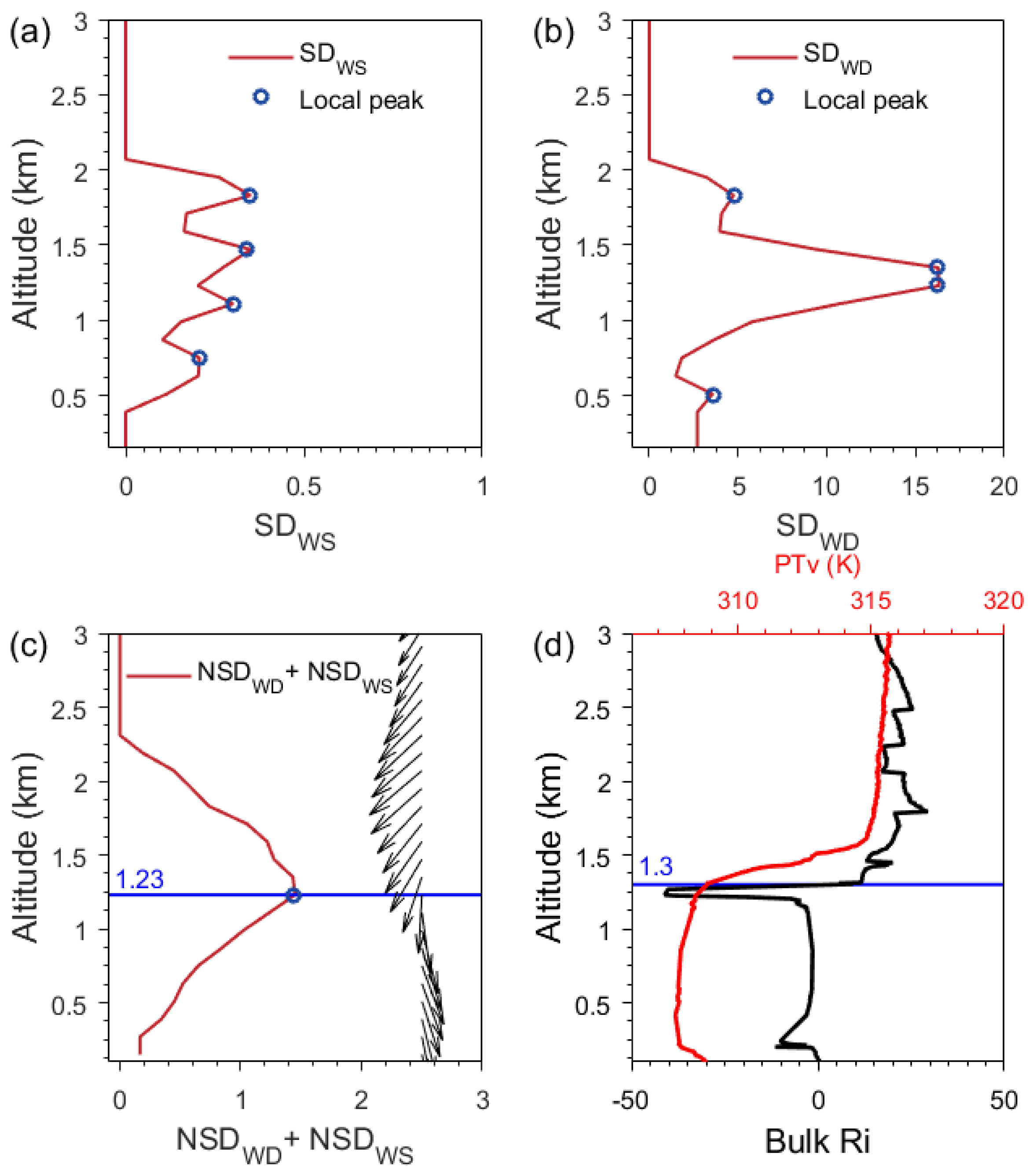
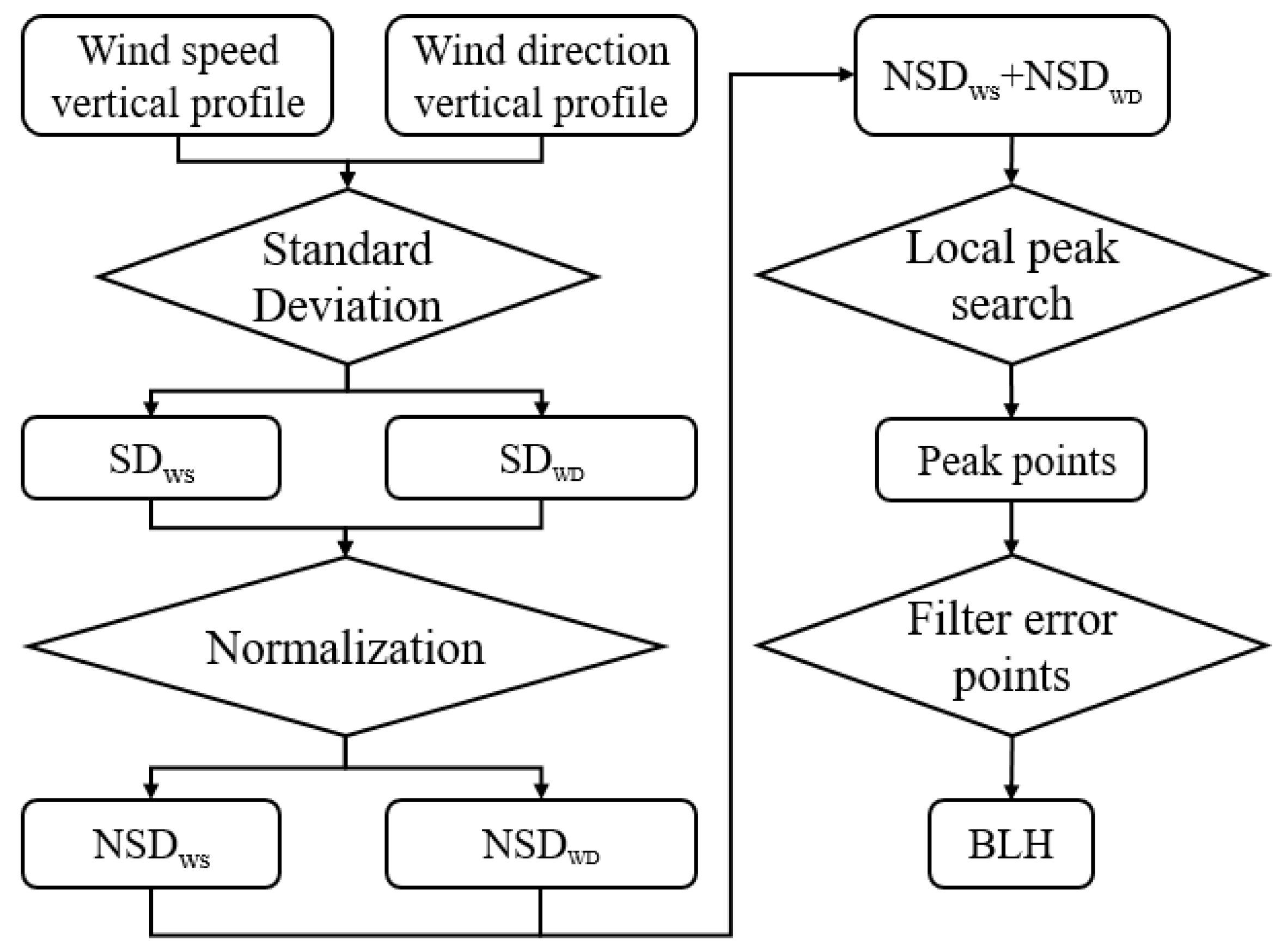
3.2. Normalized Standard Deviation Method

The NSDM was developed based on the profile of horizontal wind speed and direction. The horizontal wind speed and direction of turbulent wind are slightly different from those of laminar wind. Moreover, turbulence intensity is related to horizontal wind speed and direction. Therefore, the profiles of horizontal wind speed and direction were used to locate turbulent boundaries. To obtain the mutation information in the vertical direction, the vertical standard deviation of horizontal wind speed and direction were calculated over three adjacent altitude bins. The red lines in Figure 1a,b represent the vertical standard deviation of horizontal wind speed and direction, and the blue circles represent local peaks. SD_WS and SD_WD were used to evaluate the turbulence intensity difference between adjacent altitude bins. However, the order of magnitude of SD_WD was considerably larger than that of SD_WS. Therefore, SD_WS and SD_WD were normalized by the max normalization method. This normalization can be expressed as follows:

$$\{\begin{array}{c}\mathrm{N}\mathrm{S}{\mathrm{D}}_{\mathrm{W}\mathrm{S}}=\mathrm{S}{\mathrm{D}}_{\mathrm{W}\mathrm{S}}/\mathrm{m}\mathrm{a}\mathrm{x}\left(\mathrm{S}{\mathrm{D}}_{\mathrm{W}\mathrm{S}}\right)\\ \\ \mathrm{N}\mathrm{S}{\mathrm{D}}_{\mathrm{W}\mathrm{D}}=\mathrm{S}{\mathrm{D}}_{\mathrm{W}\mathrm{D}}/\mathrm{m}\mathrm{a}\mathrm{x}\left(\mathrm{S}{\mathrm{D}}_{\mathrm{W}\mathrm{D}}\right)\end{array}$$

(1)

where SD_WS and SD_WD represent the standard deviation of horizontal wind speed and direction in the vertical direction, respectively; max(SD_WS) and max(SD_WD) represent the maximum values in SD_WS and SD_WD, respectively; and NSD_WS and NSD_WD represent the normalized standard deviation of horizontal wind speed and direction, respectively. In Figure 1c, the profile of NSD_WS + NSD_WD was used to describe the turbulence intensity difference in the vertical direction. Local peak points (blue circles in Figure 1c) indicate strong turbulence differences between altitude bins. This can be understood as the critical point of strong and weak turbulence or of turbulence and laminar flow. The BLH result (blue line) could be determined based on the local peak point. Figure 1d displays the BLH result of RS measurement. The blue line represents BLH at 1300 m, which is similar to the RWP result (1230 m).

To clarify the process of the algorithm, more cases are shown in Figure 2 under different wind vertical structures. Strong wind shear was defined when the deviation of the horizontal wind direction between adjacent sample points exceeded 45°. According to the amount of strong wind shear, vertical wind profiles were divided into three categories: one wind shear, multiple wind shears, and no wind shear. When only one local peak existed in the NSD_WS + NSD_WD profile, the height of the local peak was output as BLH regardless of the wind structure change. Figure 2a–c illustrate that under the three wind structures, the only peak point was directly regarded as the BLH. By contrast, local peaks were filtered when multiple local peaks formed in the NSD_WS + NSD_WD profile. Multiple local peaks would be formed in the vertical direction (blue circles in Figure 2d,e,g) due to the turbulent motion pattern of the ABL and the turbulence in the cumulus and free atmosphere, particularly clear-sky turbulence [4]. That is, turbulence within or above the boundary layer resulted in the appearance of multiple local peaks. Therefore, BLH should be determined from multiple local peaks. Fortunately, previous research has shown that the near-surface maximum of radial velocity variance and near-surface minimum curvature of wind speed profiles are good criteria for determining BLH under a stable boundary layer [12,43]. The vertical flux of the component of horizontal momentum and vertical velocity variance can be used to estimate BLH for a weakly stable boundary layer [12,47,48]. Therefore, a filter was designed based on vertical variation of the wind structure. This filter is used to determine whether significant wind shear occurred at the local peak point. The height of the local peak point where significant wind shear occurred was output as BLH. Figure 2d reveals a case with multiple local peaks and one wind shear. The height of the local peak point, which corresponded to strong wind shear, was regarded as the BLH. When either no or multiple evident wind shears occurred, vertical velocity variance in the height of the local peak point was compared, and the local peak point close to the near-surface local minimum of vertical velocity variance was output as the BLH. Figure 2e demonstrates the case with multiple local peaks and no corresponding wind shear. By comparison, Figure 2g shows the condition with multiple local peaks and corresponding multiple strong wind shears. In these cases, the standard deviation of vertical velocity should filter the error points. The near-surface local minimum of vertical velocity variance is consistent with the BLH [13,45]. Therefore, the local peak point closest to the near-surface local minimum was indicated as the BLH (Figure 2f,h).

3.3. Uncertainty Analysis

Figure 3 shows a flowchart of the standard deviation method. Four key steps of this method were identified: standard deviation of wind profiles, normalization of standard deviation, local peak search, and filtration of the error point. The uncertainty of this algorithm comes from two aspects, data precision and the filter model. First, given the accuracy of wind profile data, the accuracy of the wind profile directly affects the accuracy of BLH. The location of the boundary is based on the wind speed and direction profiles. Thus, for various instruments at different sites, errors of collected data directly lead to errors in the determined BLH. The uncertainty of the horizontal wind speed and direction is approximately 5%–10% [49]. Therefore, the uncertainty of the resulting BLH is approximately 5%–10%. Second, the filter also introduces errors. For multiple local peaks, an empirical model is used to set the filter and consequently find the BLH. However, the empirical model is suitable for most situations, but not at all cases. If the case fails to conform to the empirical model, then the BLH result of this method is unreliable. Notably, a convective cloud is accompanied by strong turbulence, which results in its boundary being misjudged as BLH. Therefore, this method is unsuitable for convective cloud conditions.

3.4. Analytical Method

The atmospheric ventilation coefficient can be characterized by the BLH and wind speed in the boundary layer (WS_BL). Following Liu et al. [50], the VC was calculated as follows:

$$\mathrm{V}\mathrm{C}=\mathrm{B}\mathrm{L}\mathrm{H}\times \mathrm{W}{\mathrm{S}}_{\mathrm{B}\mathrm{L}}$$

(2)

$$\mathrm{W}{\mathrm{S}}_{\mathrm{B}\mathrm{L}}=\frac{1}{\mathrm{n}}{\displaystyle \sum }_{\mathrm{i}=1}^{\mathrm{i}=\mathrm{n}}\mathrm{W}{\mathrm{S}}_{\mathrm{i}}$$

(3)

where WS_BL is the average WS within ABL, calculated by Equation (3); BLH is the boundary layer height; and WS_i is the WS observed at a certain height.

4. Results and Discussion

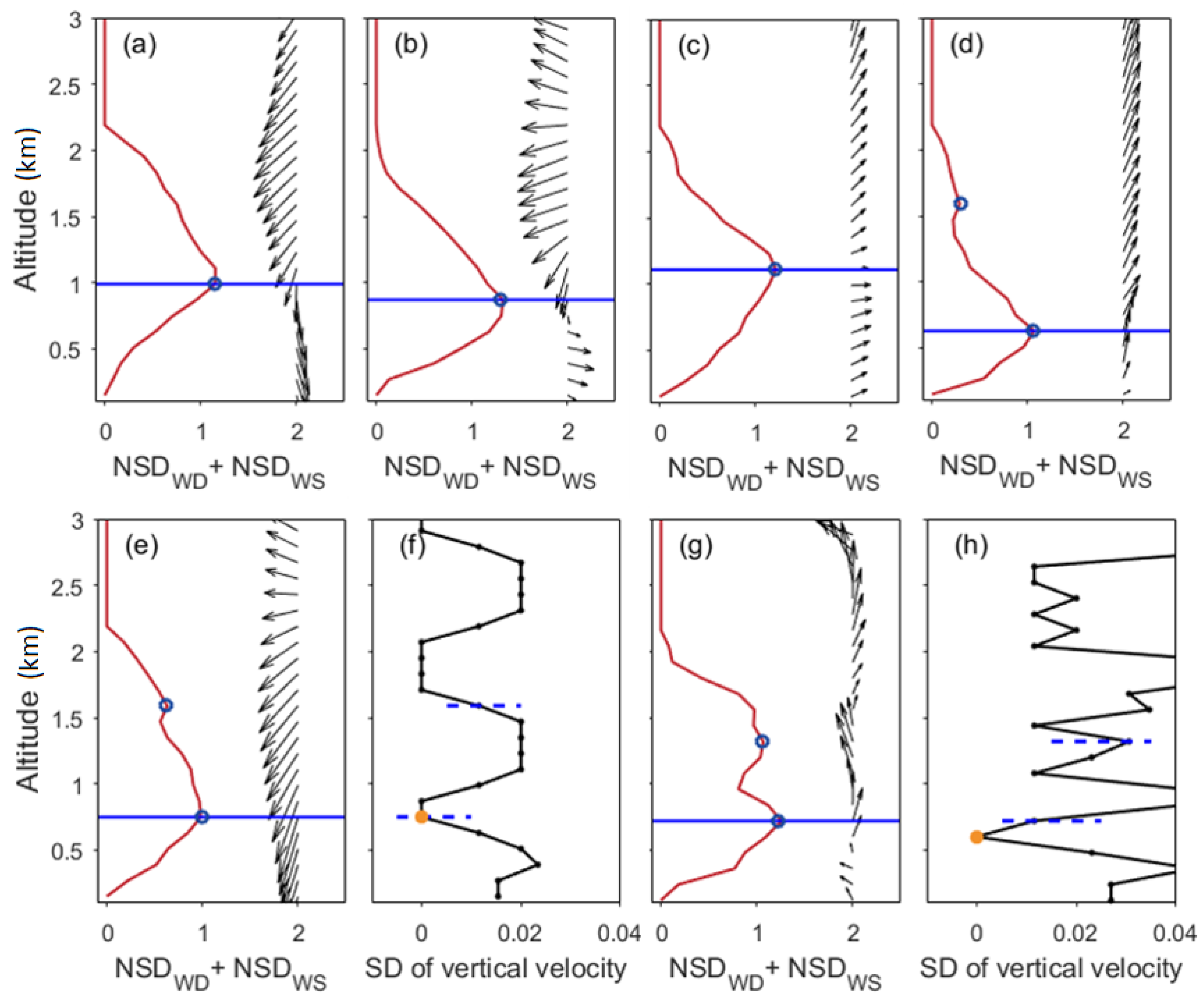
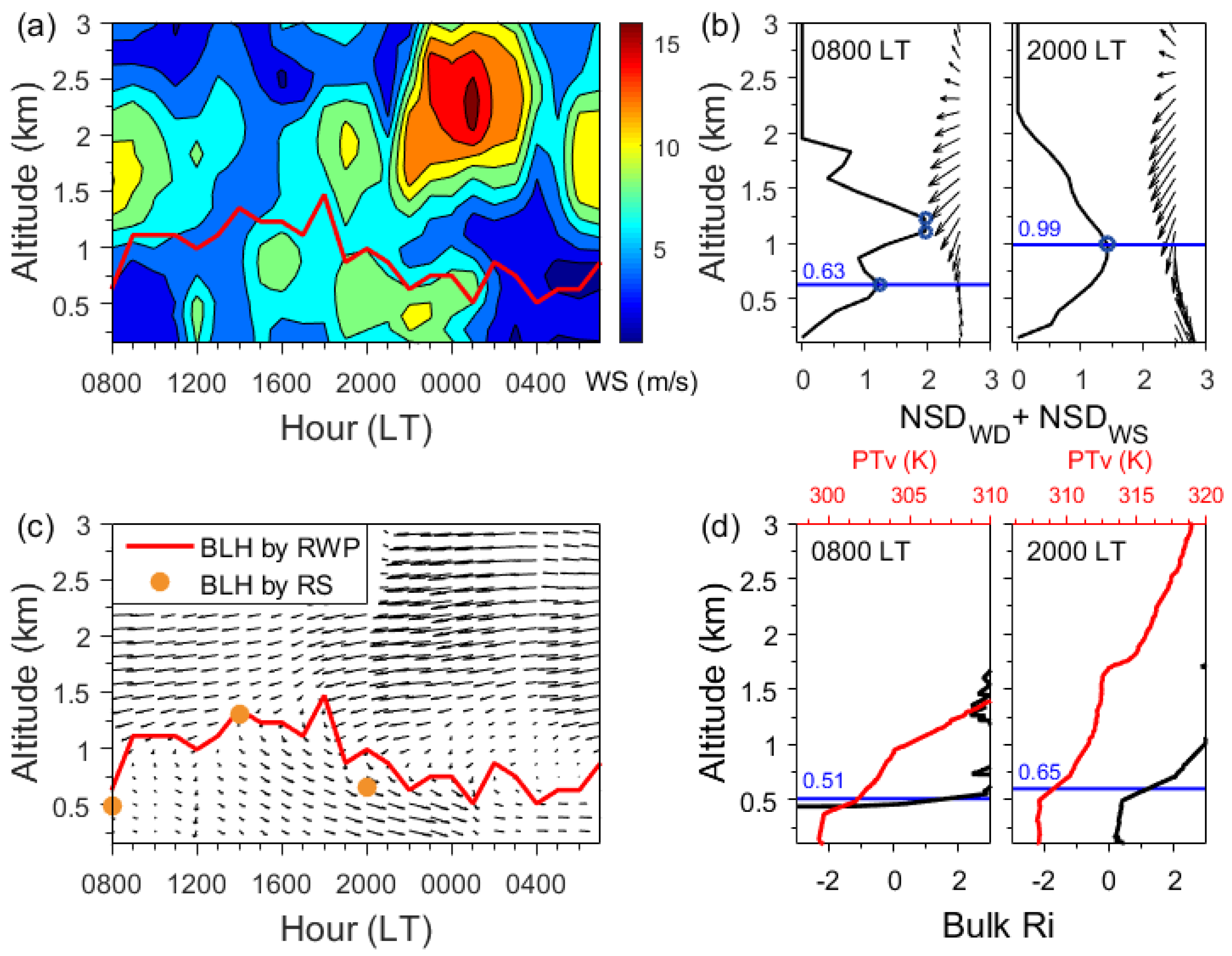
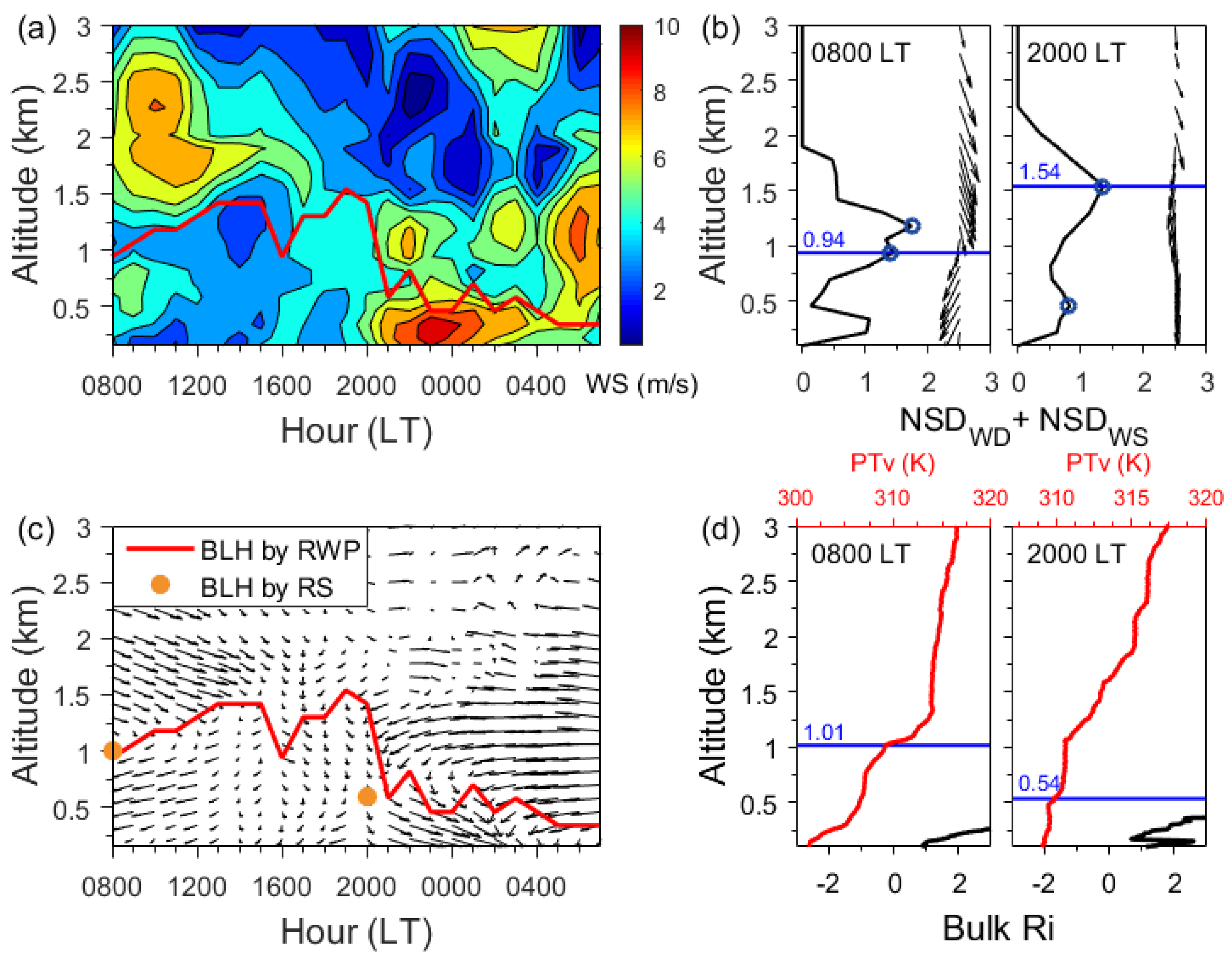
In this section, we test the feasibility and evaluate the performance of the algorithm. Furthermore, we investigate the variation of boundary layer meteorology in different cities during the summer season. Finally, we analyze the influence of surface air pollution on the vertical structure of the wind field and BLH.

4.1. Case studies

Figure 4 and Figure 5 present the case studies for BLH obtained from RWPs in BJ and NJ, respectively. Correspondingly, BLH determined from the temperature profiles was used to compare with BLH estimated from RWPs. Figure 4 reports the case study on 11 June 2019 over the BJ site; wind speed is shown in Figure 4a. Evident wind shear was revealed in the profiles of NSD_WD + NSD_WS at 08:00 and 20:00 LT, where corresponding BLHs were 630 and 990 m, respectively (Figure 4b). Evidently, a clear demarcation zone of wind vector fields between ABL and free troposphere, which roughly corresponds to the ABL height, was observed (Figure 4c). Bulk Ri and virtual potential temperature profiles from RS measurements at 08:00 and 20:00 LT are presented in Figure 4d. The local gradient maximum of virtual potential temperature profiles was consistent with the results of the Ri method. The BLH from RSs at 08:00 LT was 510 m, which was similar to the 630 m determined from RWPs. However, for 08:00 LT, the BLH from RSs (650 m) was less than that determined from RWPs (990 m). The RS observation at 14:00 LT was conducted at the BJ site during summer. The BLH from RSs at 14:00 LT was 1331 m, which is consistent with the 1350 m determined from RWPs.

The algorithm was also tested at the NJ site. Notably, the vertical resolution of this station was 120 m from 0 to 2 km, but shifted to 240 m above 2 km. The distribution of BLH over the NJ site was mostly less than 2 km [37,51]. Hence, the change in vertical resolution above 2 km did not significantly influence the estimation results. Figure 5 illustrates the case on 3 June 2019 at the NJ site. The BLHs from RWPs at 08:00 and 20:00 LT were 940 and 1540 m, respectively. BLH by RS measurement was calculated from the local gradient of the virtual potential temperature profile instead of bulk Ri. The BLH from RS (1010 m) was consistent with that determined from RWPs at 08:00 LT (940 m). However, for 20:00 LT, the BLH by RS (540 m) was different from the RWP-derived BLH (1540 m) due to the instability of the boundary layer structure at 20:00 LT, resulting in measurement differences. From the vertical distribution of NSD_WD + NSD_WS at 20:00 LT (Figure 5b), one of the local peaks (blue circle) corresponded to the BLH by RS, but due to the change in the vertical structure of the wind vector, the BLH by RWPs was located at 1540 m.

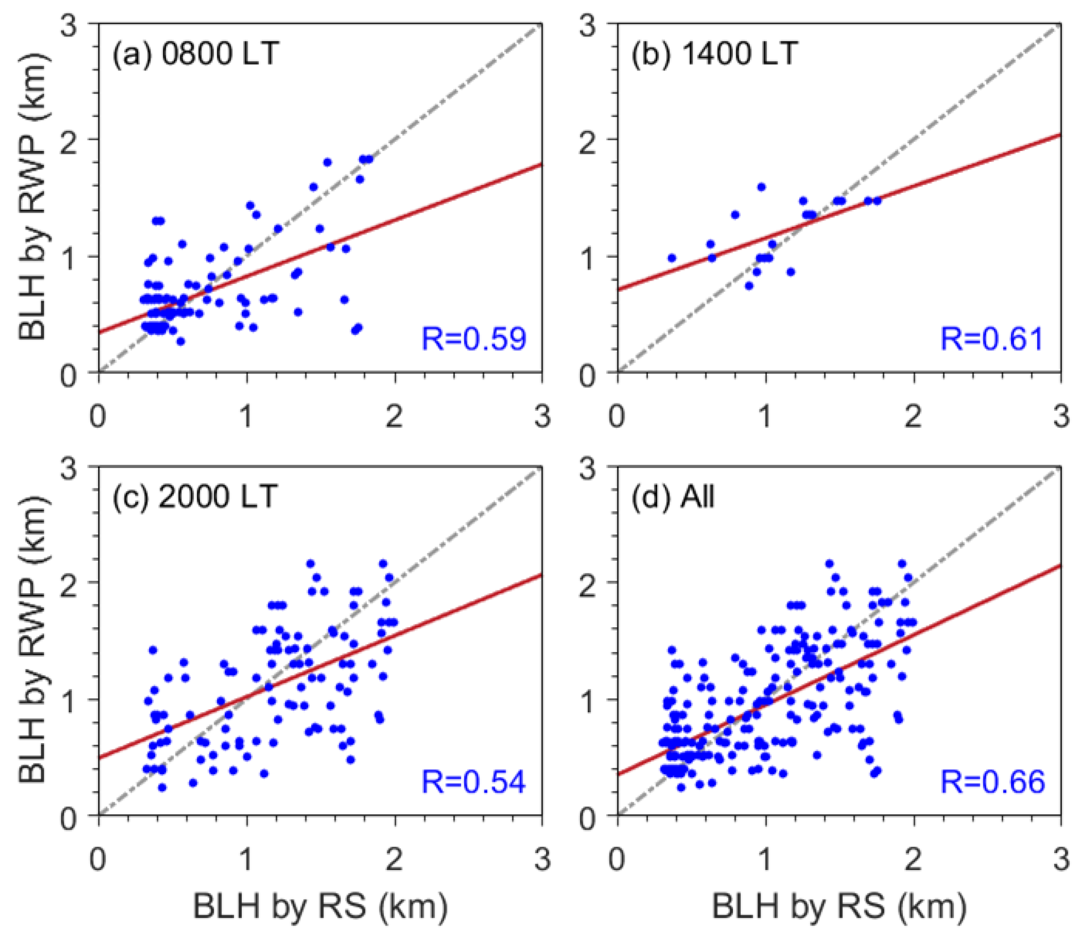
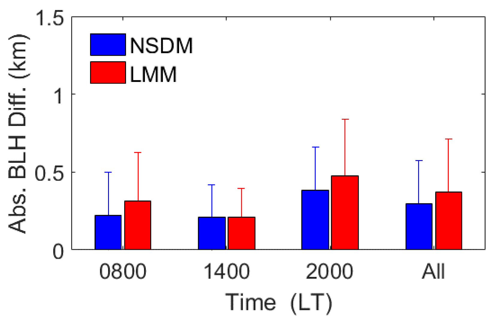
4.2. Evaluation of BLH Estimates

To evaluate the BLH estimations, BLH at 08:00, 14:00, and 20:00 LT from RWPs by NSDM were compared with corresponding BLH from RS. A total of 298 sample points were used to conduct the comparison analysis. Figure 6 shows that the correlation coefficients between BLH from RWPs and RSs at 08:00, 14:00, and 20:00 LT were 0.59, 0.61, and 0.54, respectively. For all collected data, the correlation coefficient between BLH determined by NSDM and RSs was 0.66. The results indicate that the NSDM can be applied to these radar wind profilers. Moreover, the local maxima method (LMM) was employed to compare with the NSDM. The LMM defines the largest local maximum of hourly SNR profile as BLH [15]. Figure 7 shows the mean absolute difference of BLH determined using NSDM and LMM relative to BLH determined by RS. At 14:00 LT, the difference of NSDM was similar to that of LMM. At 08:00, 20:00 LT, and all cases, the difference of NSDM was less than that of LMM. Overall, the estimation results determined by NSDM were close to the estimation results of RS, and the performance of NSDM was better than LMM. However, certain errors remained. The difference between BLH determined by NSDM and RSs reached more than 1 km in some cases. RWPs rely on the vertical structure of wind fields to invert the BLH, but the RS is dependent on the thermodynamic structure to invert the BLH [22,46]. Therefore, the difference in measurement principle may be the major cause of the difference.

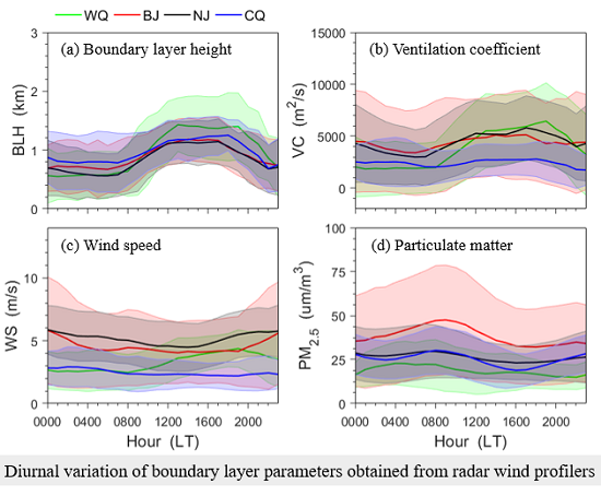
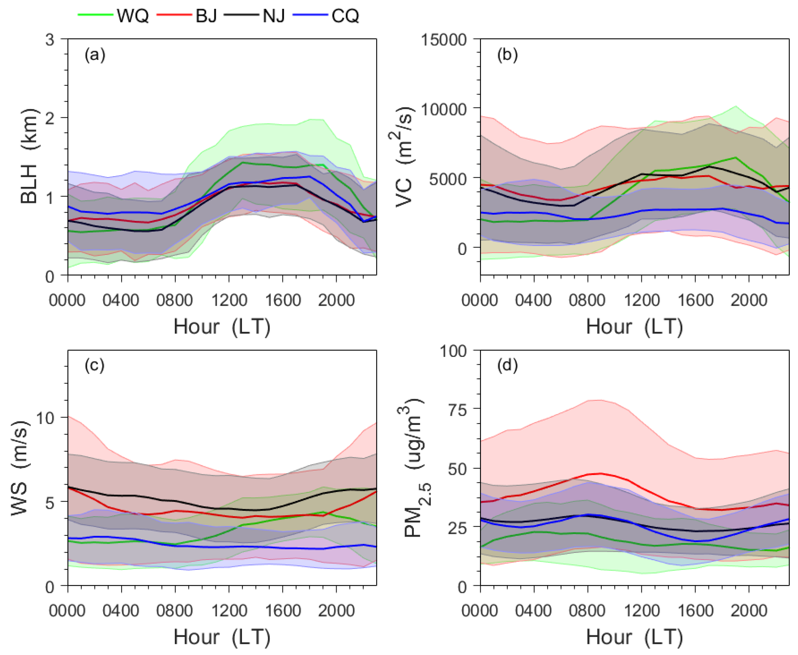
4.3. Variations of Boundary Layer Meteorology

In this section, we analyze the variations of boundary layer meteorology, such as BLH, VC, WS_BL, and surface PM_2.5 concentration at the four sites using the developmental algorithm. BLH and WS_BL represent the vertical and horizontal atmospheric dilution capability, and VC represents the atmospheric dilution capability. These parameters significantly affect the accumulation and diffusion of air pollutants [51,52].

Figure 8 presents diurnal variations of BLH, VC, WS, and PM_2.5 concentrations at the four sites averaged over the whole time period analyzed here. BLH exhibited strong daily variation characteristics, with low values at nighttime that increased rapidly after sunrise (Figure 8a). Peak BLH values commonly appeared in the afternoon (approximately 13:00–17:00 LT). For high-altitude areas such as WQ, the hourly average BLH in the daytime was larger than that at other sites, and the maximum hourly average value reached 1.426 km. For the other sites, diurnal variations of BLH were similar. Figure 8b reports the diurnal variation of VC at four sites. For BJ, NJ, and WQ, the diurnal variation in VC was similar to that of BLH. Hence, the dilution capability was strong before sunset; gradually weakened after sunset, and remained stable at night. The daily maximum VC value of at those sites was larger than 5000 m²/s. However, for CQ, the variation of VC was stable and changed between 2000 and 3000 m²/s. Combined with the ABL (Figure 8c), WS could reach up to 5 m/s in plain areas such as BJ and NJ. WS could reach a relatively high value in the daytime even for WQ. However, the WS in CQ was lower than at other sites, at less than 3 m/s throughout the day. This finding was probably because the CQ site is part of a mountainous landform and the terrain blocks the circulation of the surface atmosphere, thereby reducing the atmospheric dilution capability. Overall, the atmospheric dilution capability was strong in plain areas (BJ and NJ) during the daytime, and horizontal dilution was dominant at night. In CQ, vertical dilution was dominant during the daytime, and the atmospheric dilution capability was weak at night. In WQ, vertical dilution during the daytime was the main component.

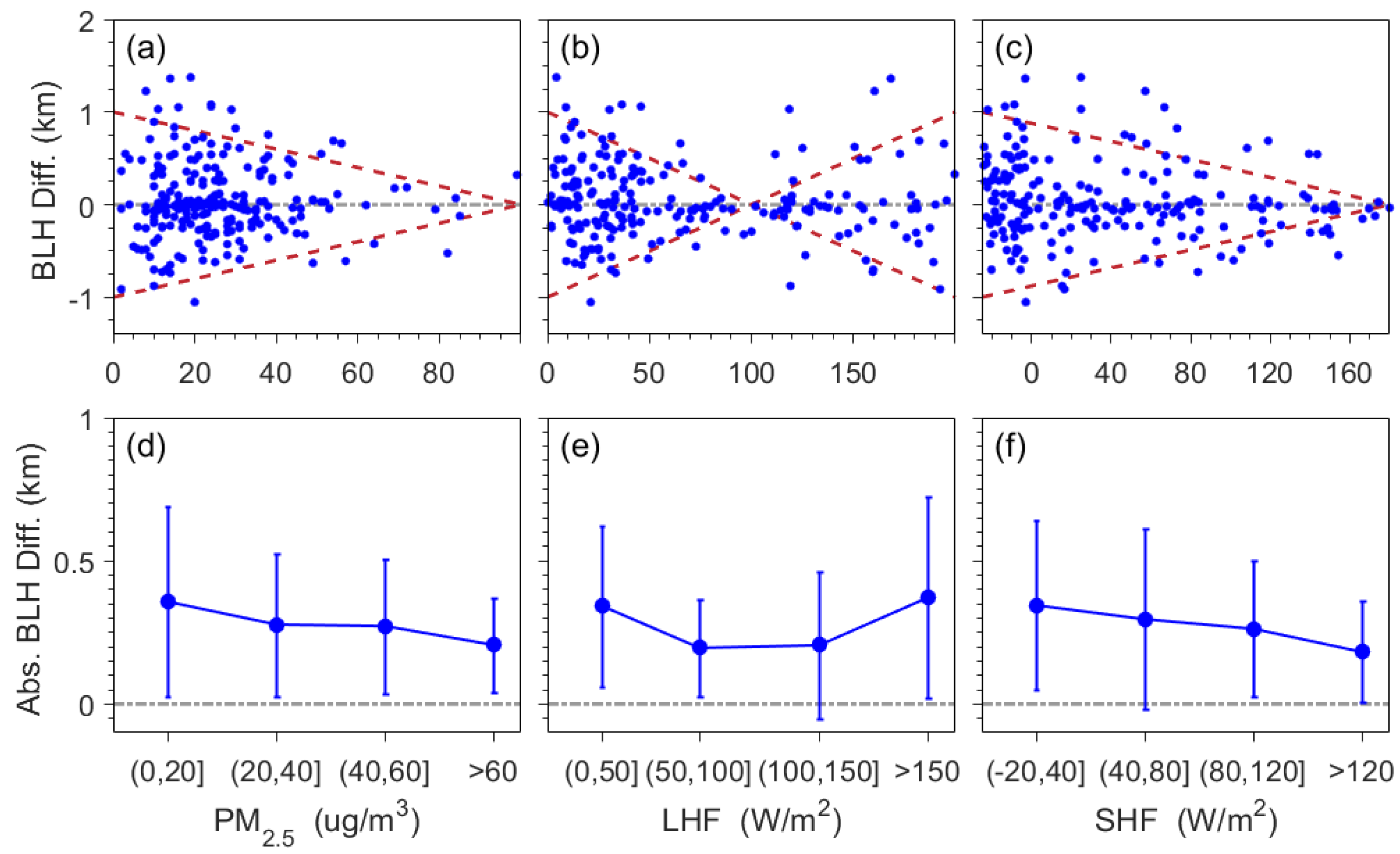
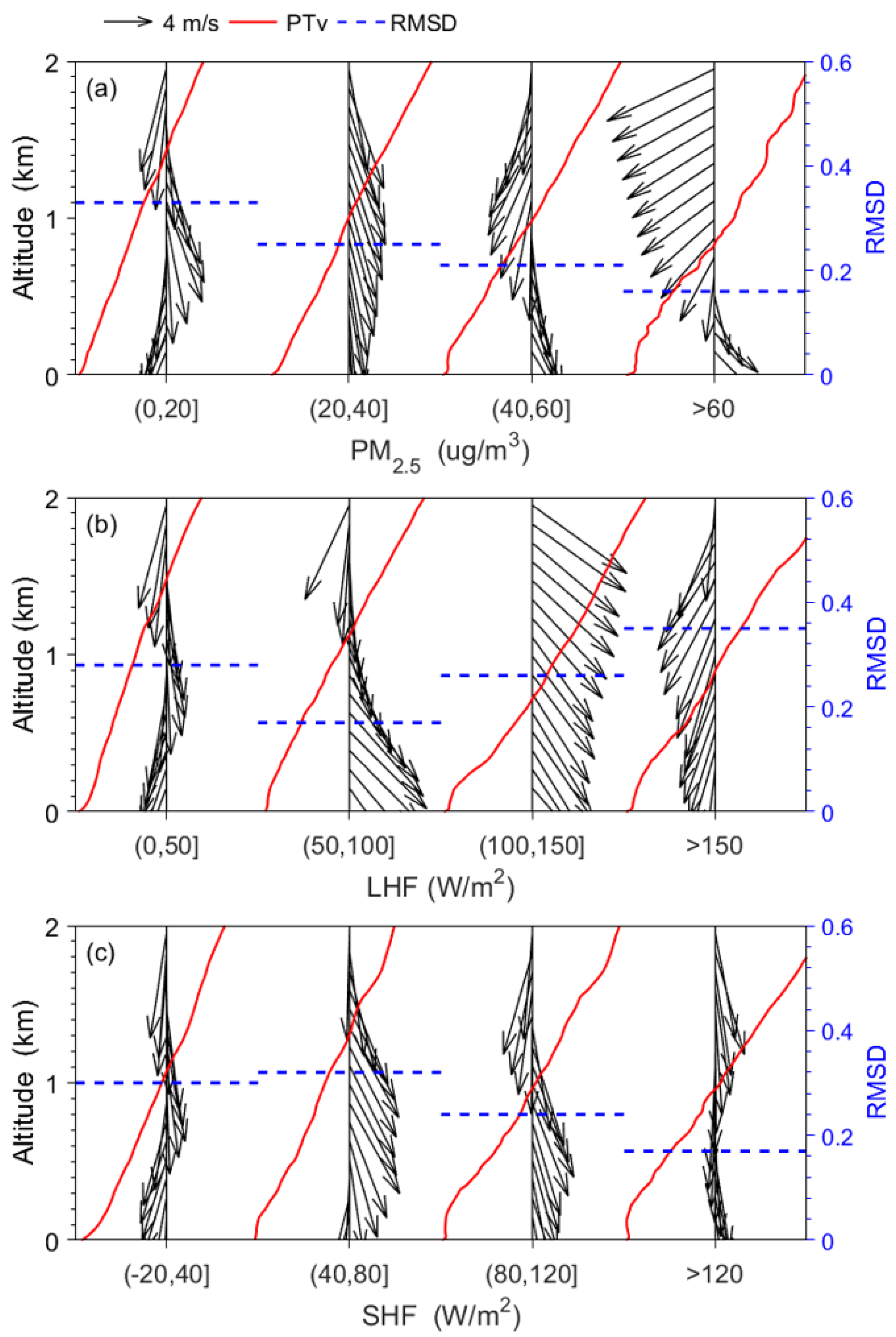
4.4. Effects of Surface Parameters

In this section, the surface SHF, LHF, and PM_2.5 concentrations data are collected to study their effects on the estimates of BLH.

Figure 9 shows the difference in BLH from RSs and RWPs between all four sites under different surface parameters. Results indicate that the height difference decreased as PM_2.5 concentration increased (Figure 9a). Similarly, Figure 9c reveals that the height difference tended to drop when SHF increased. By contrast, the height difference initially decreased and subsequently increased as the LHF increased (Figure 9b). To quantify their effects, the difference of BLH from RSs and RWPs under different conditions was calculated. Figure 9d reveals that the largest difference reached up to 0.35 ± 0.33 km when PM_2.5 concentration was less than 20 μg/m³. The smallest BLH difference of 0.2 ± 0.16 km occurred when the PM_2.5 concentration was greater than 60 μg/m³. By comparison, the smallest difference was 0.19 ± 0.17 km when the LHF lay within the range of 50 to 100 W/m² (Figure 9e). The difference of BLH became larger than 0.3 when the LHF lay in other value ranges. Interestingly, the difference tended to decline as the SHF increased. In particular, the smallest BLH difference (0.18 ± 0.17 km) occurred when the SHF was larger than 120 W/m². As a side note, BLH from RSs is based on vertical thermodynamic structures, whereas BLH from RWPs mainly relies on vertical structures of wind [7,18]. It is well known that different methods and instruments will inevitably lead to differences in BLH estimates to varying degrees [53]. Given the results shown in Figure 9, the difference between RSs and RWPs of less than 0.3 km can be considered acceptable. However, under extreme conditions such as low PM_2.5 and SHF, or extreme high or low LHF, the difference of BLH seems to be too large, and the influential mechanism merits further analysis based on model simulation in the future.

To understand the effect of these parameters, the vertical and thermodynamic structures of wind fields under different atmospheric conditions were investigated. Figure 10 demonstrates the vertical distribution of wind fields and virtual potential temperature (PT_v) under different surface PM_2.5, LHF, and SHF. Figure 10a indicates that the wind shear and PT_v gradient profiles became more evident as PM_2.5 increased. This result is similar to those in previous studies; polluted days were usually accompanied by significant atmospheric stratification [54]. As shown in Figure 9, the difference of BLH from RSs and RWPs was insignificant when the vertical wind profile exhibited strong wind shear and the PT_v profile had a strong gradient. Similarly, Figure 10b shows that the LHF was within the range of 50–100 W/m², wind shear was evident, and certain gradient change in the PT_v profile existed. This condition had the smallest mean absolute deviation. A similar situation was observed for SHF (Figure 10c). The appearance of wind shear was consistent with that of the gradient in the PT_v profile when the SHF was larger than 80 W/m², thereby leading to a small mean absolute deviation. Therefore, the BLH determined from RWPs was only consistent with that from RSs when wind shear and the PT_v profile gradient existed simultaneously. This finding is explained given that the surface parameters affect the vertical and thermodynamic structures of wind fields. The RWP relies on wind shear to invert the BLH. However, the RS is dependent on the thermodynamic structure to invert the BLH. Therefore, the height difference between the BLH from RSs and RWPs is only evident when the vertical field or thermodynamic structures of the wind are unstable. The results of the effects of surface parameters on atmospheric vertical structure provide new insights for the application of RWP BLH observations.

5. Conclusions

Using continuous high-temporal resolution wind measurements from RWPs in BJ, NJ, CQ, and WQ, we developed an adaptive method to estimate BLH from the vertical structure of wind fields. This algorithm is advantageous over previously developed algorithms, since it can calculate BLH without assuming initial parameters such as threshold and window function.

The proposed method was applied to continuous RWP measurements at the BJ, NJ, CQ, and WQ sites during the summer. To assess the accuracy of this method, a comprehensive comparison was conducted between BLH determined from RSs and from RWPs. The results indicate that the correlation coefficient between BLH retrievals from RWPs and from RSs was 0.66. However, in some cases, the difference between BLH from RWPs and from RSs reached more than 1 km. To understand the differences, the effects of surface SHF, LHF, and PM_2.5 concentration on the accuracy of BLH from RWPs were subsequently investigated. The results show that their height difference decreased as PM_2.5 concentration increased, while the same phenomenon was observed for SHF. The height difference initially decreased and subsequently increased as the LHF increased. Moreover, the diurnal variation of summertime boundary layer meteorology at the four sites was examined. Results revealed that the boundary layer exhibited clear diurnal variations, and the atmospheric dilution capability had significant regional differences. For the BJ, NJ, and WQ sites, the dilution capability was strong before sunset, gradually weakened after sunset, and remained stable at night. The maximum hourly mean VC at BJ, NJ, and WQ was larger than 5000 m²/s. However, for CQ, the variation of hourly mean VC was stable, changing between 2000 and 3000 m²/s.

We propose an adaptive method in an attempt to estimate BLH from high-resolution RWP measurements in BJ, NJ, CQ, and WQ. The proposed algorithm can provide reasonable estimates of BLH from the vertical structure of wind fields. The findings of this study provide key references for ABL-related research using large-scale RWP measurements. However, this algorithm cannot be applied when the vertical structure of the wind field is disordered and when either multiple or no strong wind shear would cause uncertain errors. Therefore, much work will be needed in the future to improve the algorithm. For example, we can try to improve the performance of the algorithm by combining deep learning methods. Afterward, efforts will be devoted to estimating BLH using the vast wealth of height-revolved wind from the well-established RWP network in China.

References

1. Ku, J.Y.; Mao, H.; Zhang, K.; Civerolo, K.; Rao, S.T.; Philbrick, C.R.; Clark, R. Numerical investigation of the effects of boundary-layer evolution on the predictions of ozone and the efficacy of emission control options in the northeastern United States. Environ. Fluid Mech. 2001, 1, 209–233. [Google Scholar] [CrossRef]
2. Tang, G.; Zhu, X.; Hu, B.; Xin, J.; Wang, L.; Münkel, C.; Wang, Y. Impact of emission controls on air quality in Beijing during APEC 2014: Lidar ceilometer observations. Atmos. Chem. Phys. 2015, 15, 12667–12680. [Google Scholar] [CrossRef] [Green Version]
3. Garratt, J.R. The atmospheric boundary layer. Earth-Sci. Rev. 1994, 37, 89–134. [Google Scholar] [CrossRef]
4. Stull, R.B. An Introduction to Boundary Layer Meteorology; Springer Science & Business Media: Berlin, Germany, 1988. [Google Scholar]
5. Wang, W.; Mao, F.; Gong, W.; Pan, Z.; Du, L. Evaluating the governing factors of variability in nocturnal boundary layer height based on elastic lidar in Wuhan. Int. J. Environ. Res. Public Health 2016, 13, 1071. [Google Scholar] [CrossRef] [PubMed] [Green Version]
6. Liu, B.; Ma, Y.; Gong, W.; Zhang, M.; Yang, J. Determination of boundary layer top on the basis of the characteristics of atmospheric particles. Atmos. Environ. 2018, 178, 140–147. [Google Scholar] [CrossRef]
7. Seibert, P.; Beyrich, F.; Gryning, S.E.; Joffre, S.; Rasmussen, A.; Tercier, P. Review and intercomparison of operational methods for the determination of the mixing height. Atmos. Environ. 2000, 7, 1001–1027. [Google Scholar] [CrossRef]
8. Tang, G.; Zhang, J.; Zhu, X.; Song, T.; Münkel, C.; Hu, B.; Xin, J. Mixing layer height and its implications for air pollution over Beijing, China. Atmos. Chem. Phys. 2016, 16, 2459–2475. [Google Scholar] [CrossRef] [Green Version]
9. Song, L.C.; Rong, G.; Ying, L.; Guo-Fu, W. Analysis of China’s haze days in the winter half-year and the climatic background during 1961–2012. Adv. Clim. Chang. Res. 2014, 5, 1–6. [Google Scholar] [CrossRef]
10. Nair, V.S.; Moorthy, K.K.; Alappattu, D.P.; Kunhikrishnan, P.K.; George, S.; Nair, P.R.; Niranjan, K. Wintertime aerosol characteristics over the Indo-Gangetic Plain (IGP): Impacts of local boundary layer processes and long-range transport. J. Geophys. Res. Atmos. 2007, 112. [Google Scholar] [CrossRef]
11. Miao, Y.; Guo, J.; Liu, S.; Liu, H.; Li, Z.; Zhang, W.; Zhai, P. Classification of summertime synoptic patterns in Beijing and their associations with boundary layer structure affecting aerosol pollution. Atmos. Chem. Phys. 2017, 17, 3097–3110. [Google Scholar] [CrossRef] [Green Version]
12. LeMone, M.A.; Tewari, M.; Chen, F.; Dudhia, J. Objectively determined fair-weather CBL depths in the ARW-WRF model and their comparison to CASES-97 observations. Mon. Weather Rev. 2013, 141, 30–54. [Google Scholar] [CrossRef] [Green Version]
13. LeMone, M.A.; Tewari, M.; Chen, F.; Dudhia, J. Objectively determined fair-weather NBL features in ARW-WRF and their comparison to CASES-97 observations. Mon. Weather Rev. 2014, 142, 2709–2732. [Google Scholar] [CrossRef] [Green Version]
14. Dolman, B.K.; Reid, I.M.; Tingwell, C. Stratospheric tropospheric wind profiling radars in the Australian network. EarthPlanets Space 2018, 70, 170. [Google Scholar] [CrossRef] [Green Version]
15. Molod, A.; Salmun, H.; Dempsey, M. Estimating planetary boundary layer heights from NOAA profiler network wind profiler data. J. Atmos. Ocean. Technol. 2015, 32, 1545–1561. [Google Scholar] [CrossRef]
16. Ishihara, M.; Kato, Y.; Abo, T.; Kobayashi, K.; Izumikawa, Y. Characteristics and performance of the operational wind profiler network of the Japan Meteorological Agency. J. Meteorol. Soc. Jpn. 2006, 84, 1085–1096. [Google Scholar] [CrossRef] [Green Version]
17. Nash, J.; Oakley, T.J. Development of COST 76 wind profiler network in Europe. Phys. Chem. Earth Part. B 2001, 3, 193–199. [Google Scholar] [CrossRef]
18. Liu, B.; Ma, Y.; Guo, J.; Gong, W.; Zhang, Y.; Mao, F.; Li, J.; Guo, X.; Shi, Y. Boundary layer heights as derived from ground-based Radar wind profiler in Beijing. IEEE Trans. Geosci. Remote Sens. 2019. [Google Scholar] [CrossRef]
19. Singh, N.; Solanki, R.; Ojha, N.; Janssen, R.H.; Pozzer, A.; Dhaka, S.K. Boundary layer evolution over the central Himalayas from radio wind profiler and model simulations. Atmos. Chem. Phys. 2016, 16. [Google Scholar] [CrossRef] [Green Version]
20. Compton, J.C.; Delgado, R.; Berkoff, T.A.; Hoff, R.M. Determination of planetary boundary layer height on short spatial and temporal scales: A demonstration of the covariance wavelet transform in ground-based wind profiler and lidar measurements. J. Atmos. Ocean. Technol. 2013, 30, 1566–1575. [Google Scholar] [CrossRef]
21. Bianco, L.; Wilczak, J.M.; White, A.B. Convective boundary layer depth estimation from wind profilers: Statistical comparison between an automated algorithm and expert estimations. J. Atmos. Ocean. Technol. 2008, 25, 1397–1413. [Google Scholar] [CrossRef]
22. Ottersten, H. Atmospheric structure and radar backscattering in clear air. Radio Sci. 1969, 4, 1179–1193. [Google Scholar] [CrossRef]
23. Angevine, W.M.; White, A.B.; Avery, S.K. Boundary-layer depth and entrainment zone characterization with a boundary-layer profiler. Bound.-Layer Meteorol. 1994, 68, 375–385. [Google Scholar] [CrossRef]
24. Cohn, S.A.; Angevine, W.M. Boundary layer height and entrainment zone thickness measured by lidars and wind-profiling radars. J. Appl. Meteorol. 2000, 39, 1233–1247. [Google Scholar] [CrossRef]
25. Bianco, L.; Wilczak, J.M. Convective boundary layer depth: Improved measurement by Doppler radar wind profiler using fuzzy logic methods. J. Atmos. Ocean. Technol. 2002, 19, 1745–1758. [Google Scholar] [CrossRef]
26. Angevine, W.M.; Ecklund, W.L.; Carter, D.A.; Gage, K.S.; Moran, K.P. Improved radio acoustic sounding techniques. J. Atmos. Ocean. Technol. 1994, 11, 42–49. [Google Scholar] [CrossRef] [Green Version]
27. Bian, J. Intercomparison of humidity and temperature sensors: GTS1, Vaisala RS80, and CFH. Adv. Atmos. Sci. 2011, 28, 139–146.s. [Google Scholar] [CrossRef]
28. Zhai, P.; Eskridge, R.E. Atmospheric water vapor over China. J. Clim. 1997, 10, 2643–2652. [Google Scholar] [CrossRef]
29. Liu, B.; Ma, Y.; Gong, W.; Zhang, M.; Shi, Y. The relationship between black carbon and atmospheric boundary layer height. Atmos. Pollut. Res. 2019, 10, 65–72. [Google Scholar] [CrossRef]
30. Liu, B.; Ma, Y.; Shi, Y.; Jin, S.; Jin, Y.; Gong, W. The characteristics and sources of the aerosols within the nocturnal residual layer over Wuhan, China. Atmos. Res. 2020, 241, 104959. [Google Scholar] [CrossRef]
31. Guo, J.; Xia, F.; Liu, H.; Lou, M.; He, J.; Zhang, Y.; Wang, F.; Min, M.; Zhai, P. Impact of diurnal variability and meteorological factors on the PM2.5-AOD relationship: Implications for PM2.5 remote sensing. Environ. Pollut. 2017, 221, 94–104. [Google Scholar] [CrossRef] [Green Version]
32. Gage, K.S.; Williams, C.R.; Ecklund, W.L. UHF wind profilers: A new tool for diagnosing tropical convective cloud systems. Bull. Am. Meteorol. Soc. 1994, 75, 2289–2294. [Google Scholar] [CrossRef] [Green Version]
33. Williams, C.R.; Ecklund, W.L.; Gage, K.S. Classification of precipitating clouds in the tropics using 915-MHz wind profilers. J. Atmos. Ocean. Technol. 1995, 12, 996–1012. [Google Scholar] [CrossRef]
34. Lou, M.J.; Guo, L.; Wang, H.; Xu, D.; Chen, Y.; Miao, Y.; Lv, Y.; Li, X.; Guo, S.; Ma, J.L. On the relationship between aerosol and boundary layer height in summer in China under different thermodynamic conditions. Earth Space Sci. 2019, 6, 887–901. [Google Scholar] [CrossRef] [Green Version]
35. Zhang, W.; Guo, J.; Miao, Y.; Liu, H.; Song, Y.; Fang, Z.; He, J.; Lou, M.; Yan, Y.; Li, Y.; et al. On the summertime planetary boundary layer with different thermodynamic stability in China: A radiosonde perspective. J. Clim. 2018, 31, 1451–1465. [Google Scholar] [CrossRef]
36. Guo, J.; Li, Y.; Cohen, J.B.; Li, J.; Chen, D.; Xu, H.; Liu, L.; Yin, J.; Hu, K.; Zhai, P. Shift in the temporal trend of boundary layer height trend in China using long-term (1979–2016) radiosonde data. Geophys. Res. Lett. 2019, 46, 6080–6089. [Google Scholar] [CrossRef] [Green Version]
37. Guo, J.; Miao, Y.; Zhang, Y.; Liu, H.; Li, Z.; Zhang, W.; He, J.; Lou, M.; Yan, Y.; Bian, L.; et al. The climatology of planetary boundary layer height in China derived from radiosonde and reanalysis data. Atmos. Chem. Phys. 2016, 16, 13309. [Google Scholar] [CrossRef] [Green Version]
38. Gelaro, R.; McCarty, W.; Suárez, M.J.; Todling, R.; Molod, A.; Takacs, L.; Wargan, K. The modern-era retrospective analysis for research and applications, version 2 (MERRA-2). J. Clim. 2017, 30, 5419–5454. [Google Scholar] [CrossRef]
39. GMAO. MERRA-2 tavg1_2d_flx_Nx: 2d, 1-Hourly, Time-Averaged, Single-Level, Assimilation, Surface Flux Diagnostics V5.12.4. GES DISC. 2015. Available online: https://0-scholar-google-com.brum.beds.ac.uk/scholar?hl=en&as_sdt=0%2C5&q=MERRA-2+tavg1_2d_flx_Nx%3A+2d%2C+1-hourly%2C+time-averaged%2C+singlelevel%2C+assimilation%2C+surface+flux+diagnostics+V5.12.4.+GES+DISC&btnG (accessed on 15 June 2019).
40. Helfand, H.M.; Schubert, S.D. Climatology of the simulated Great Plains low-level jet and its contribution to the continental moisture budget of the United States. J. Clim. 1995, 8, 784–806. [Google Scholar] [CrossRef]
41. Stevens, R.J.; Verzicco, R.; Lohse, D. Radial boundary layer structure and Nusselt number in Rayleigh–Bénard convection. J. Fluid Mech. 2010, 643, 495–507. [Google Scholar] [CrossRef] [Green Version]
42. Le Bouar, E.; Petitdidier, M.; Lemaitre, Y. Retrieval of ageostrophic wind from a radiosounding network and a single ST radar. Q. J. R. Meteorol. Soc. 1998, 124, 2435–2464. [Google Scholar] [CrossRef]
43. Pichugina, Y.L.; Banta, R.M. Stable boundary layer depth from high-resolution measurements of the mean wind profile. J. Appl. Meteorol. Climatol. 2010, 49, 20–35. [Google Scholar] [CrossRef]
44. Pichugina, Y.L.; Tucker, S.C.; Banta, R.M.; Brewer, W.A.; Kelley, N.D.; Jonkman, B.J.; Newsom, R.K. Horizontal-velocity and variance measurements in the stable boundary layer using Doppler lidar: Sensitivity to averaging procedures. J. Atmos. Ocean. Technol. 2008, 25, 1307–1327. [Google Scholar] [CrossRef]
45. Vickers, D.; Mahrt, L. Evaluating formulations of stable boundary layer height. J. Appl. Meteorol. 2004, 43, 1736–1749. [Google Scholar] [CrossRef] [Green Version]
46. Kurzeja, R.J.; Berman, S.; Weber, A.H. A climatological study of the nocturnal planetary boundary layer. Bound. -Layer Meteorol. 1991, 54, 105–128. [Google Scholar] [CrossRef]
47. Kosović, B.; Curry, J.A. A large eddy simulation study of a quasi-steady, stably stratified atmospheric boundary layer. J. Atmos. Sci. 2000, 57, 1052–1068. [Google Scholar] [CrossRef] [Green Version]
48. Vogelezang, D.H.P.; Holtslag, A.A.M. Evaluation and model impacts of alternative boundary-layer height formulations. Bound.-Lay. Meteorol. 1996, 81, 245–269. [Google Scholar] [CrossRef]
49. Liu, B.; Guo, J.; Gong, W.; Shi, L.; Zhang, Y.; Ma, Y. Characteristics and performance of vertical winds as observed by the radar wind profiler network of China. Atmos. Meas. Tech. Discuss. 2020. in review. [Google Scholar] [CrossRef]
50. Liu, Y.; Tang, G.; Zhou, L.; Hu, B.; Liu, B.; Li, Y.; Wang, Y. Mixing layer transport flux of particulate matter in Beijing, China. Atmos. Chem. Phys. 2019, 19, 9531–9540. [Google Scholar] [CrossRef] [Green Version]
51. Yin, J.; Gao, C.Y.; Hong, J.; Gao, Z.; Li, Y.; Li, X.; Zhu, B. Surface Meteorological Conditions and Boundary Layer Height Variations During an Air Pollution Episode in Nanjing, China. J. Geophys. Res. Atmos. 2019, 124, 3350–3364. [Google Scholar] [CrossRef]
52. Molod, A.; Salmun, H.; Marquardt Collow, A.B. Annual Cycle of Planetary Boundary Layer Heights Estimated From Wind Profiler Network Data. J. Geophys. Res. Atmos. 2019, 124, 6207–6221. [Google Scholar] [CrossRef]
53. Seidel, D.J.; Ao, C.O.; Li, K. Estimating climatological planetary boundary layer heights from radiosonde observations: Comparison of methods and uncertainty analysis. J. Geophys. Res.-Atmos. 2010, 115. [Google Scholar] [CrossRef] [Green Version]
54. Liu, B.; Ma, Y.; Gong, W.; Zhang, M.; Yang, J. Study of continuous air pollution in winter over Wuhan based on ground-based and satellite observations. Atmos. Pollut. Res. 2018, 9, 156–165. [Google Scholar] [CrossRef]
Figure 1. Illustration of the boundary layer height (BLH) detection algorithm: (a) profiles of standard deviation of horizontal wind speed (SDWS) and corresponding detected local peaks; (b) profiles of standard deviation of horizontal wind direction (SDWD) and corresponding detected local peaks; (c) profiles of horizontal wind (black arrows) and normalized standard deviations of horizontal wind speed and wind direction (NSDWS + NSDWD, respectively; in red); and (d) profiles of virtual potential temperature (PTv; in red) and bulk Richardson number (Ri; in black) at 06:00 UTC on 11 June 2019. Blue circles and blue lines represent local peaks and BLH, respectively.
Remotesensing 12 01657 g001
Figure 2. Typical wind vertical structures in different time periods. Profiles of NSDWS and NSDWD over BJ station at (a) 05:00 UTC and (b) 21:00 UTC on 11 June 2019, and (c) 04:00 UTC and (d) 00:00 UTC on 10 June 2019. Profiles of (e) NSDWD + NSDWS and (f) vertical velocity variance at 12:00 UTC on 7 June 2019 over BJ station. (g) NSDWD + NSDWS and (h) vertical velocity variance at 21:00 UTC on 17 June 2019 over WQ station. Black arrows indicate wind vectors; blue circles and lines represent local peaks and BLH, respectively.
Remotesensing 12 01657 g002
Figure 3. Flowchart of standard deviation method used to estimate the BLH from radar wind profilers (RWPs).
Remotesensing 12 01657 g003
Figure 4. Case study on 11 June 2019 over BJ station. (a) Time-height cross-section of wind speed and BLH estimated from RWPs. (b) Vertical distribution of NSDWD + NSDWS at 08:00 and 20:00 local time (LT, UTC+8). (c) Time–height cross-section of wind vector and BLH estimated from RWPs (red lines) and BLH from radiosondes (RSs; orange points). (d) Vertical distribution of bulk Ri and virtual potential temperature (PTv) at 08:00 and 20:00 LT. Blue, red, and black lines represent BLH, PTv, and Ri, respectively.
Remotesensing 12 01657 g004
Figure 5. Case study on 11 June 2019 over NJ station. (a) Time-height cross-section of wind speed and BLH estimated from RWPs. (b) Vertical distribution of NSDWD + NSDWS at 08:00 and 20:00 local time (LT, UTC+8). (c) Time–height cross-section of wind vector and BLH estimated from RWPs (red lines) and BLH from radiosondes (RSs; orange points). (d) Vertical distribution of bulk Ri and virtual potential temperature (PTv) at 08:00 and 20:00 LT. Blue, red, and black lines represent BLH, PTv, and Ri, respectively.
Remotesensing 12 01657 g005
Figure 6. Scatterplots of BLH from RS measurements vs. RWPs for all sites at (a) 08:00 local time (LT), (b) 14:00 LT, (c) 20:00 LT, and (d) all times. Gray and red lines represent 1:1 reference line and regression line, respectively. Correlation coefficients (R) are given in the lower right corner of each panel.
Remotesensing 12 01657 g006
Figure 7. Comparison of BLH determined by RWP measurements using normalized standard deviation method (NSDM, in blue) and local maxima method (LMM, in red) against radiosonde (RS).
Remotesensing 12 01657 g007
Figure 8. Diurnal variations of (a) BLH, (b) ventilation coefficient (VC), (c) wind speed in the boundary layer (WSBL), and (d) particulate matter with aerodynamic diameter ≤2.5 µm (PM2.5) at four observation stations. Green, red, black, and blue lines represent WQ, BJ, NJ, and CQ sites, respectively. Corresponding color shading areas represent one standard deviation of each variable analyzed here.
Remotesensing 12 01657 g008
Figure 9. Difference of BLH between RS and RWP measurements between all four sites shown as a function of (a,d) surface PM2.5 concentration, (b,e) latent heat flux (LHF), and (c,f) sensible heat flux (SHF).
Remotesensing 12 01657 g009
Figure 10. Vertical distribution of wind (black arrows) and virtual potential temperature (PTv, in red) shown as a function of (a) surface PM2.5 concentration, (b) LHF, and (c) SHF. Blue lines represent root mean squared difference (RMSD) of the difference of BLH between RWP and RS measurements at each bin.
Remotesensing 12 01657 g010