Novel Remote Sensing Index of Electron Transport Rate Predicts Primary Production and Crop Health in L. sativa and Z. mays

Abstract

Photosynthesis performance can be assessed quantitatively with light response curves. These curves record the Electron Transport Rate (ETR) as a function of light intensity. Then, statistical fit on these curves parameterize light use efficiency, maximum photosynthetic activity and the reaction of the apparatus to stress. While this technique is performed with portable fluorometers in field conditions, it is difficult to scale it to the canopy level. The Fraunhofer line discrimination technique, which detects fluorescence signals emitted during photosynthesis, is a promising method to assess photosynthetic performance of canopies. In this study, we define a remote sensing ETR index based on a combination of three parameters: sun-induced fluorescence, normalized differential vegetation index and light intensity. Two representatives of C₃ and C₄ photosynthesis, L. sativa and Z. mays, experienced a fertilization concentrations gradient. ETR increased with light intensity in both crops. In L. sativa, ETR assumed a linear relationship between the photosynthetic activity and light intensity, with a correlation of R² = 0.99 to the portable fluorometer. Additional parametrization revealed a resilience of its reaction centers to photoinhibition in maximum light intensities. When Z. mays experienced open field conditions, ETR correlated with the plant’s status. While the results of this study are promising, the index still requires validation in terms of temporal track and spatial variability.

1. Introduction

Plants harvest sunlight energy in order to perform photosynthesis [1]. However, not all energy is used in primary production [2]. The absorbed energy can have three different fates: (a) photochemistry—where light energy is used to excite electrons within the Photosystem II (PSII) and the Photosystem I (PSI) reaction centers, (b) photoprotection—energy is dissipated back to the environment as heat [3] and (c) energy is emitted back to the environment as fluorescence [4]. A successful excitation of electrons within the reaction centers occurs when an electron passes from an excited reaction center to the first acceptor within the photosynthetic electron transport chain—Quinone a (Qa). This transfer is accompanied with a change in fluorescence emitted from the apparatus and, therefore, can be quantitatively determined [5]. In fact, a successful transfer of electrons can be qualified as quantum yield of the system, i.e., the ability of PSII or PSI to perform photosynthesis in a given light intensity. When quantum yield is multiplied by the amount of light present during the measurement, the product determines the rate of electrons entering the chain [5]. Electrons moving along the chain are transferred to various locations, one of which is the Nicotine Amide DiPHosphate (NADPH) [5]. During movement along the chain, Adenosine TriPhosphate (ATP) is synthesized through photophosphorylation within the apparatus. Both parts will be used later as chemical components in the Calvin–Benson–Bassham (CBB) cycle in order to assimilate inorganic carbon into Glyceraldehyde-3-phosphate, the precursor of sugars [1]. Therefore, electron transport rate (ETR) and light response curves report indirectly on primary production.

The logarithmic behavior of the light response curve is divided into three parts (Figure 1): (a) the light limiting intensity range, where the photosynthetic rate is affected only by light intensity, (b) carbon assimilation limiting intensity range, where the photosynthetic rate depends on the assimilation rate of inorganic CO₂ and (c) the photoinhibition limiting intensity range, where the photosynthetic rate starts to decline due to a closure of reaction centers [6].

Fitting a logarithmic function to the light response curve, in turn, enables its parameterization [7]: (a) I_k—characteristic light intensity (the concave in the logarithmic function) reveals the size of light-harvesting complexes, (b) I_m—predicted light intensity, where the maximum ETR is achieved, (c) light use efficiency (LUE)—the linear part of the curve (slope) and (d) Omega—the magnitude of photoinhibition. It is, therefore, not surprising that light response curves are the method of choice to define photosynthetic performance towards environmental conditions [8]. Portable fluorometers are being used to record light response curves, yet from a very small part of one leaf, from one plant at a time [9,10]. Remote sensing techniques overcome such a limitation: powerful spectral resolution spectrometers situated above a crop measure the average signal coming back from the canopy and assess the overall fluorescence emitted [11]. This signal can be detected via the Fraunhofer line discrimination (FLD) technique [12]. This method exploits the overlap between natural atmospheric oxygen absorption lines within the reflected light and fluorescence spectrum that is emitted back to the environment from the plants.

Photosynthetic organisms have evolved to maximize carbon assimilation in their respected environments. C₃-type photosynthetic crops dominate most terrestrial ecosystems, while C₄-type photosynthesis is found in subtropical and tropical regions [13]. The main biochemical difference between C₃ and C₄ plants is the compartmentalization of the fixating CO₂ enzyme, Ribulose-1,5-bisphosphate-Carboxylase-Oxygenase (RUBISCO). In C₃-type photosynthesis, RUBISCO is located to the mesophyll chloroplasts, while in C₄-type photosynthesis, RUBISCO is located to the bundle sheaths chloroplasts [14]. In turn, there is a difference in the way RUBSICO receives the CO₂ needed for assimilation. In C₃ plants, CO₂ diffuses through the intercellular cavities into the chloroplast and RUBISCO; in C₄ plants, CO₂ is delivered into the bundle sheath chloroplast via a 2-PhosphoEnolPyruvate (PEP)-carboxylase step, which incorporates CO₂ into triose molecules. These will be shuttled to the bundle sheath chloroplasts and only then de-carboxilated and fed to the RUBISCO. Eventually, in both types of photosynthesis, RUBISCO is the ultimate stop for CO₂, which is then assimilated into the photosynthetic CO₂ reductive pathway [15]. Hence, light response curves of C₃- and C₄-type photosynthesis will behave similarly, given specific conditions.

There are only a few studies which have attempted to calculate remote sensing of ETR in the past. The difficulty to reach this index is due to understating what is included within the Sun Induced Fluorescence (SIF) signal, for example, see Reference [16]. In part, It appears that SIF directly relates to quantum yield at the leaf level [17], but, on the other hand, reports show that additional parameters are needed in order for SIF to report on quantum yield [18]. From these studies, it is understood that remotely sensed light response curves can provide additional information which is not available with a simple SIF signal acquisition. On top of that, the retrieval of SIF is possible from any airborne platform (satellites, airplanes and drones), but the recurring measurements for light response curve limit the construction of the curve along planes [19] or drones [20], due to the requirement of an overpassing frequency. The objective of this study, therefore, is to construct a remote sensing ETR index. In this study, we report on a novel formula which calculates remote sensing of ETR and light response curves. The index was calibrated on the C₃-type photosynthesis plant, L. sativa, under photoprotective conditions. These conditions enabled the apparatus to divert most energy to photochemistry at the expense of energy losses due to photoprotection. Then, we used the index to calculate crop status with a C₄-type photosynthesis plant, Z. mays.

2. Materials and Methods

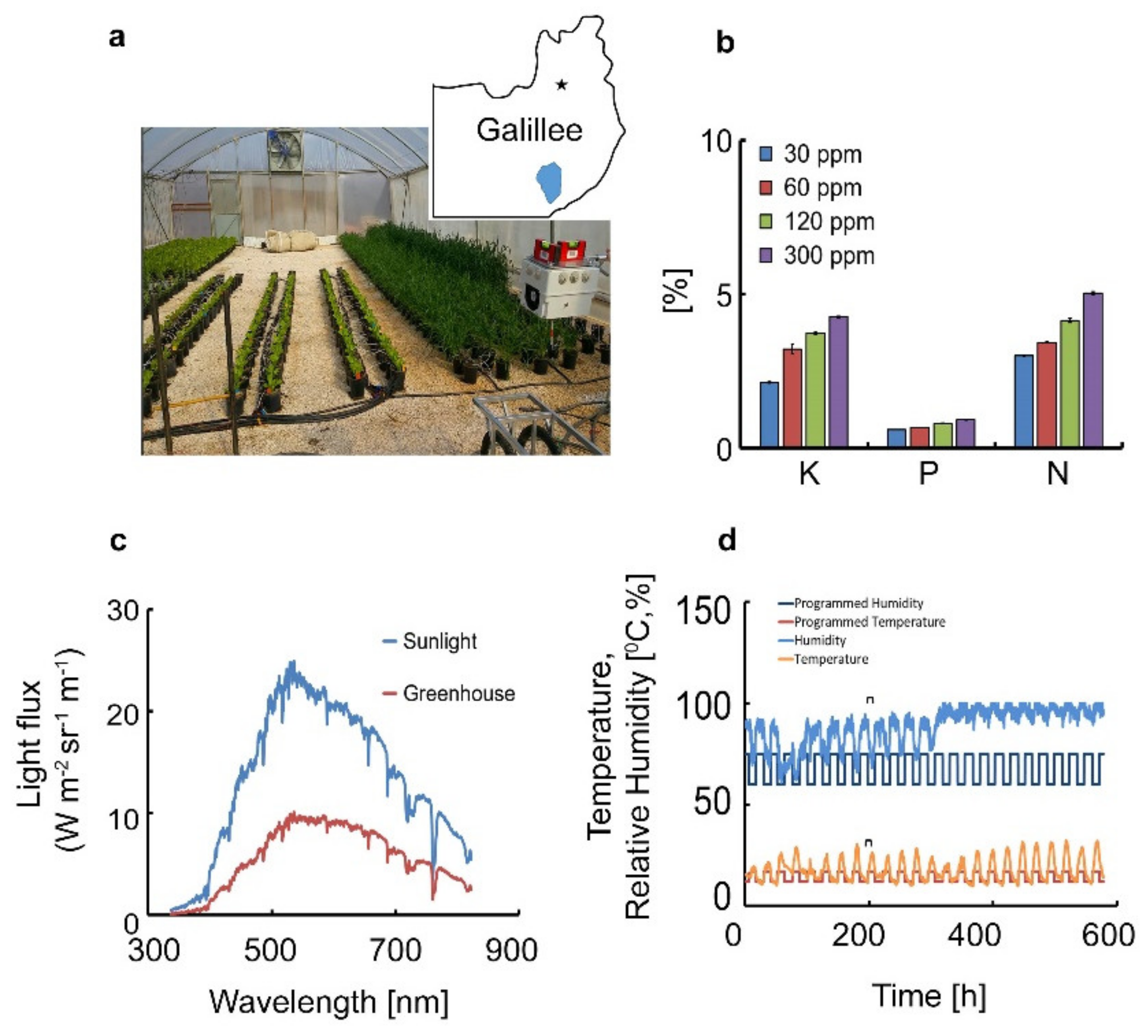
2.1. Experimental Design

We performed an experiment over one year on two crop types that are typically grown in Israel during winter and summer. While the crops were able to grow until the end of the vegetative growth, measurements were performed over a single time instance during each season per each crop. The first period was winter—a greenhouse in Havat Ma’taim (33°09′10.3″N, 35°37′23.4″E) in the Upper Galilee region in Israel and which grows L. sativa (Figure 2a). The greenhouse was covered with a scattering UltraViolet—VISual spectral range (UV-VIS) polygon sheet and a shade net which reduced light intensity by at least half (Figure 2c). The cultivation period took place during the winter of 2018, starting at 7 February 2018 until 6 March 2018. The internal climate was monitored by Galcon’s^© humidity and temperature controller (Galileo climate, Galcon, Israel), which directly controls on transparent curtains, thus maintaining the humidity and temperature at about constant conditions. Average conditions during the experimental period within the greenhouse were: Temperature^period = 17.69 ± 0.09 °C, Humidity^period = 88.5% ± 0.15%, averaged conditions during experiment: Temperature^instance = 17.56 ± 0.40 °C, Humidity^instance = 83.17% ± 0.59%. The second period was summer—under open field conditions in Havat Gadash located at 33°10′48.7″N 35°34′58.5″E, in proximity to the other experimental site. The cultivation period in open field conditions took place during summer of 2017, starting at 6 September 2017 until 29 November 2017, with Z. mays ‘super sweet’ (sh2). Averaged conditions during the experiment in open field were: Temperature^period = 21.52 ± 0.15 °C, Humidity^period = 56.29% ± 0.42%, during the experiment: Temperature^instance = 26.17 ± 1.00 °C, Humidity^instance = 61.38% ± 2.80%.

2.2. Fertilization Treatments

L. sativa was potted in 2 L pots with 80% peat:20% clay soil constituents (Kekkila BVB, Sweden). It was fertigated with a gradient of Shefer-1 (ICL, Haifa, Israel) liquid fertilizer with 8:3:5 K:P:N (Potassium:Phosphate:Nitrogen) + 3 µgr microelements at the following concentrations: 30, 60, 120 and 300 ppm, identified by the total nitrogen amount in the fertilizer. Each treatment consisted of 30 pots divided into 6 biological repeats (5 pots per repeat) and organized in random blocks between three rows. Thus, the experiment was arranged as 40 pots per row, 20 on each side. The Z. mays experiment was fertilized with a slow-release fertilizer Multicote^© (ICL, Haifa, Israel) 15:7:15 K:P:N + 2MgO + micronutrients in the following concentrations: Control, 6, 12, 20 and 30 g/L. Each treatment contained 30 pot quads that were ordered in 5 rows, each resembled a biological repeat and 6 pot quads per row. This experiment was part of a larger dataset where additional types of Multicote^© fertilizers were used but were omitted from analysis.

2.3. Sensors System Setup

We followed the same setup as suggested by Burkart et al. [20]. Briefly, there were two units of spectrometers (STS-microspectrometers, OceanInsight, FL, USA) designated as AIR and GROUND units. The AIR unit was either mounted on cable grids 3.5 m above the plot (Z. mays) or mounted on a trolley 2.5 m above (L. sativa). The GROUND unit was situated above a 94% white reflective panel (Permaflect^©, Labsphere, USA). The readings of both spectrometers were simultaneously taken. Reflectance spectrums were constructed according to the spectrometers manufacturer’s instructions and Pavia et al. [21]. Spectral data acquisition occurred at the following time instances per each crop: (a) L. sativa—07:00 a.m. (4.2 W m⁻²), 08:30 a.m. (33.2 W m⁻²), 10:30 a.m. (185.5 W m⁻²), 12:00 p.m. (225.3 W m⁻²); (b) Z. mays—07:00 a.m. (187.2 W m⁻²), 10:30 a.m. (447.7 W m⁻²), 11:30 a.m. (527.1 W m⁻²).

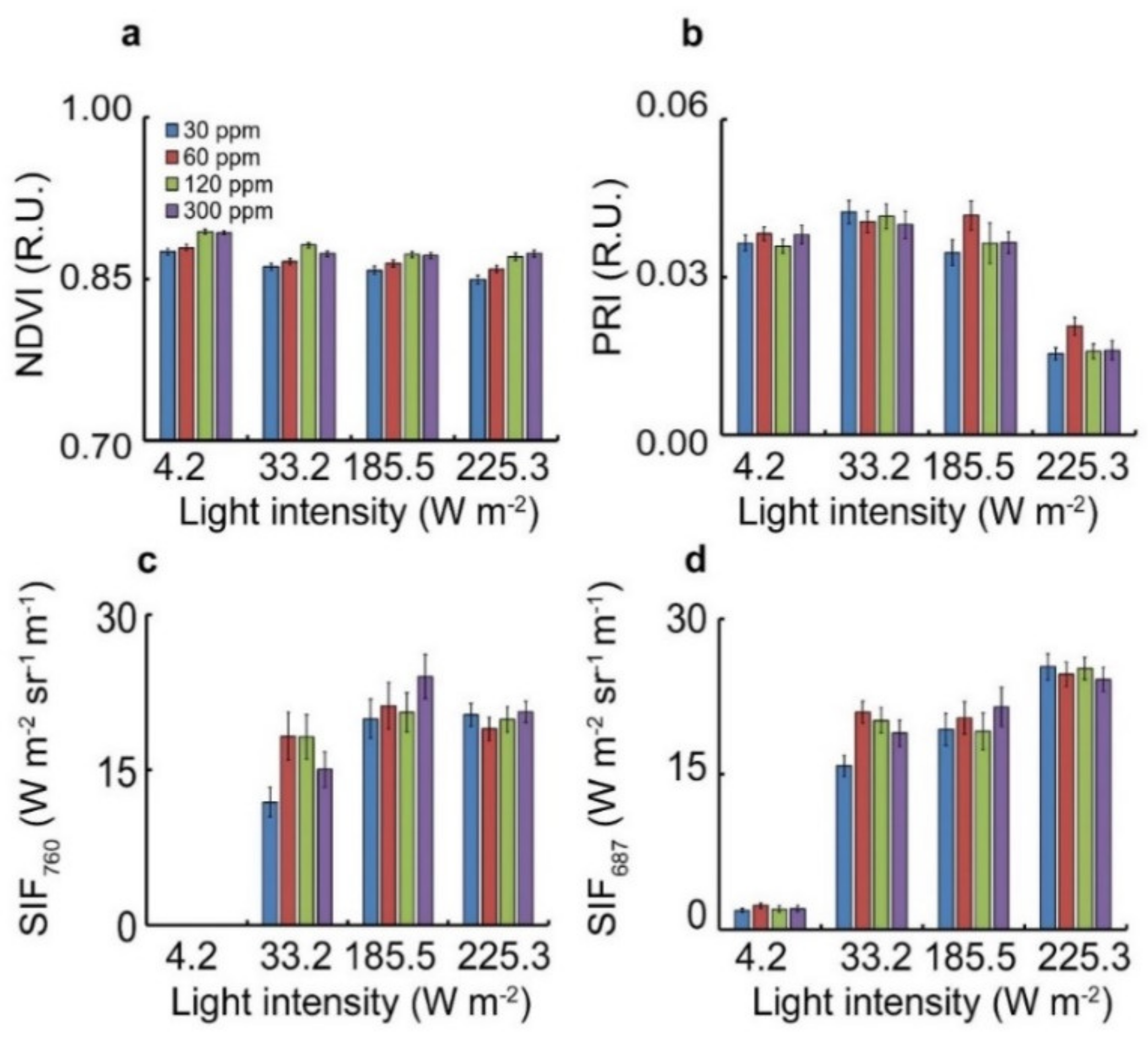
2.4. Vegetation Indices Calculation

Vegetation Indices (VIs) are a mathematical combination of two or more spectral wavelengths [22]. This study made use of two robust VIs: the normalized differential vegetation index (NDVI) [23] and the photochemical reflectance index (PRI) [24]. Originally constructed for the classification of vegetation within mixed soil/vegetation satellite images, NDVI is known to be a non-invasive yet sensitive tool for biomass and nitrogen variability within crop canopies [25]. It is, therefore, used by plant breeders in order to search for variabilities in crop yield via agronomic traits [26] or the early detection of compromised crops due to biotic stressors [27]. The PRI index is the reflectance spectrum remote sensing alternative to photoprotection detection at the leaf level. It is very sensitive to plant stress and thus used in the classification of grain yield [28] and identification of light energy stress in various crops [29]. Both of these indices belong to a large family of equations which compare the normalized difference between two wavelengths to their sum:

$$Normalized Difference=\frac{{\rho }_i-{\rho }_j}{{\rho }_i+{\rho }_j}$$

(1)

where ${\rho }_{i,j}$ are the terms describing two values of the reflectance spectrum at a designated wavelength i or j (units of spectral measurement, in this study nanometer (nm)). NDVI and PRI wavelengths used in this study are (670 nm, 800 nm) [30] and (531 nm, 570 nm), respectively.

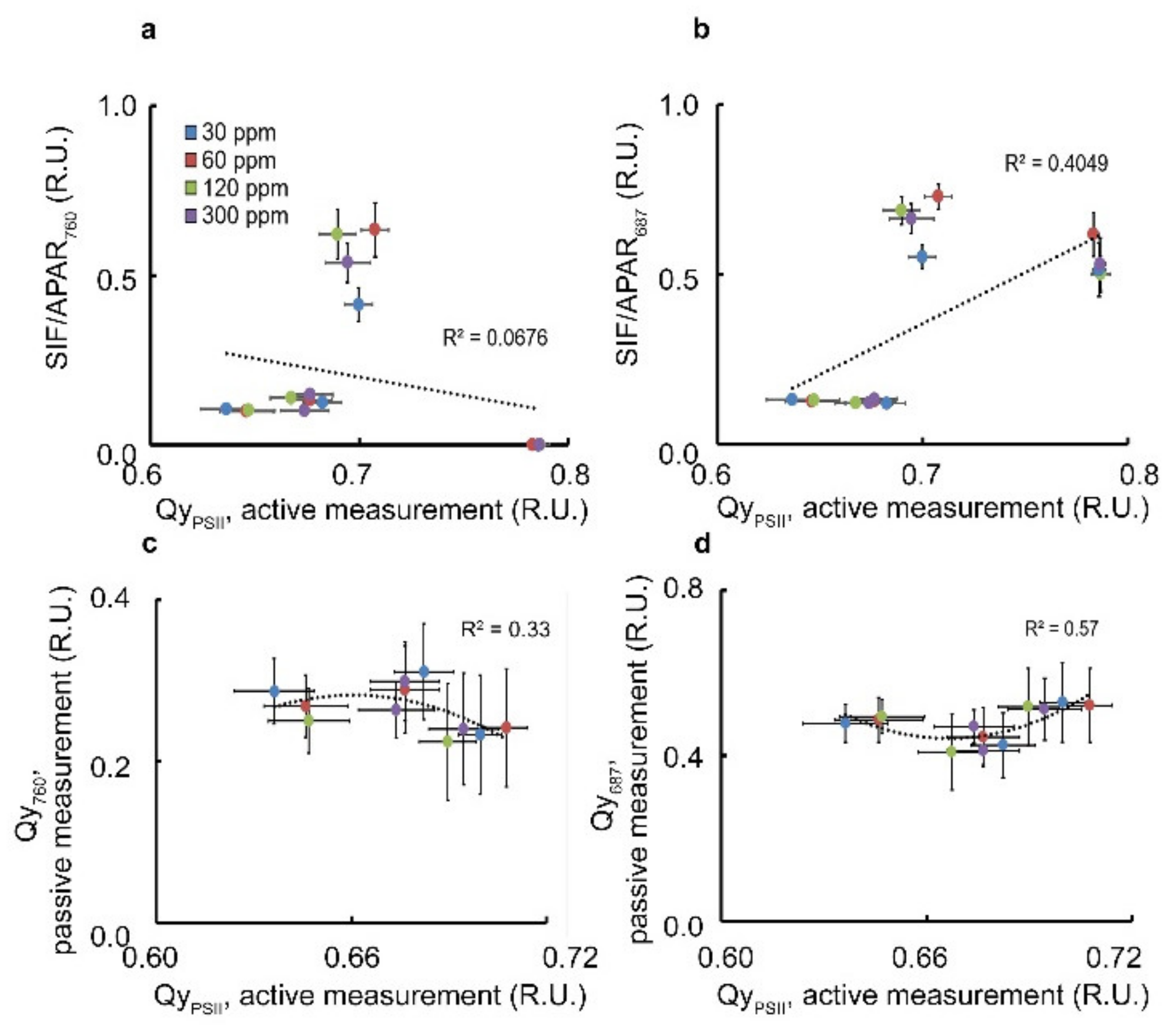
2.5. Chlorophyll Fluorescence Measurements

Active fluorescence measurements were performed with a Pulsed Amplitude Modulation (PAM) portable fluorometer (FP100-Max, Photon System Instruments, Drasov, Czech Republic) on two of the fully expanded young leaves (3–5 from top meristem) within each potted crop. Sun-induced fluorescence (SIF) was calculated as dictated by Alonso [31] in the O₂A and O₂B Fraunhofer atmospheric absorption bands.

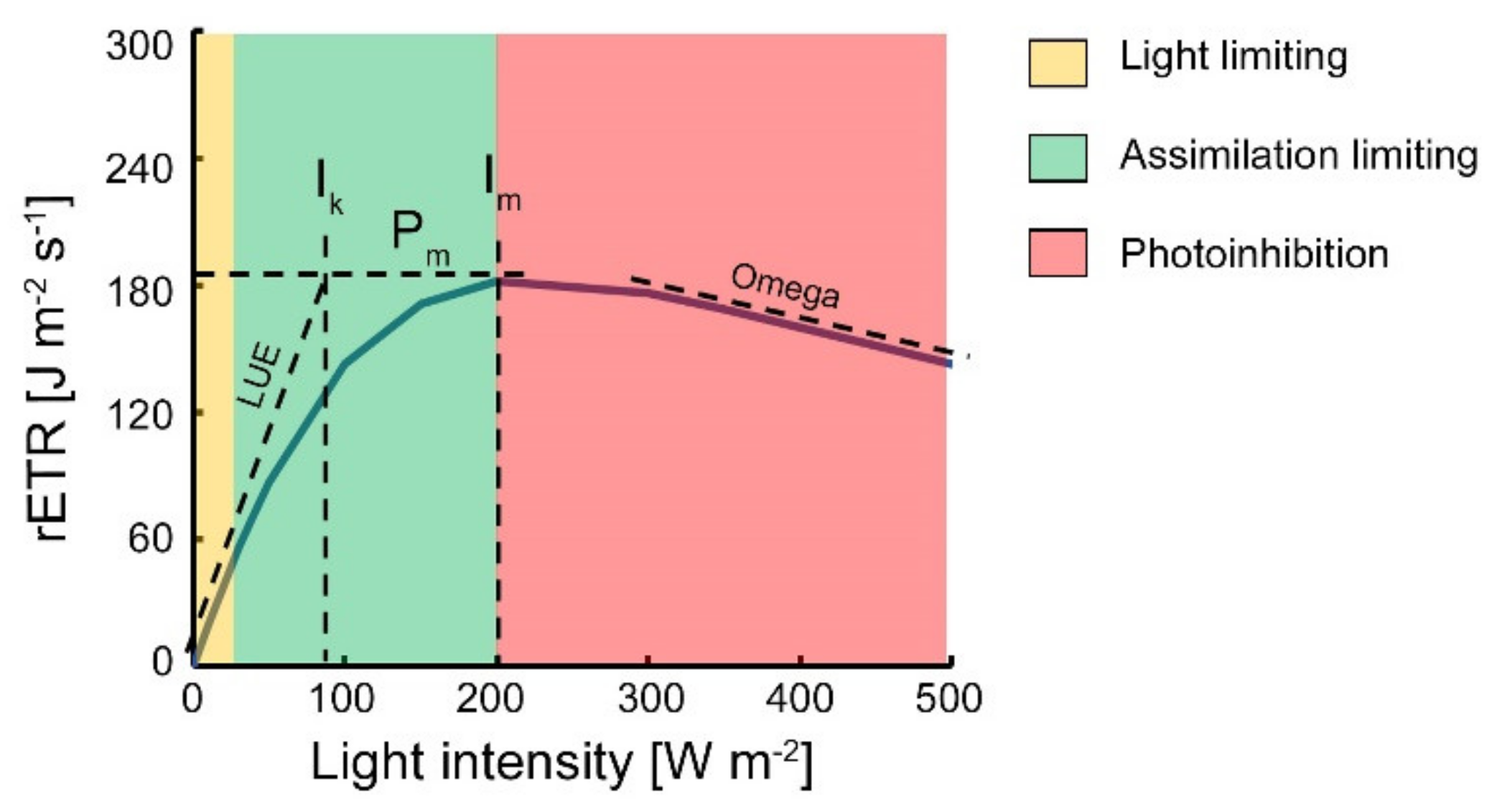
2.6. Construction of ETR Index

The ETR index was calculated by the following formulation:

$$ETR\left({\mathrm{Wm}}^{-2}\right)=\frac{SI{F}_{687}}{SI{F}_{687}+SI{F}_{760}}·NDVI·PAR\left({\mathrm{Wm}}^{-2}\right)$$

(2)

where, SIF_λ is the SIF calculated at the respected atmospheric oxygen absorption line (687 nm or 760 nm), NDVI is calculated as mentioned above and photosynthetically active radiance (PAR) values are retrieved from a local meteorological station. During investigation, we checked whether the ETR term (without the PAR argument) could be considered as a quantum yield index. For this reason, either SIF₆₈₇ or SIF₇₆₀ were used in the numerator.

2.7. Logarithmic Function Statistical Fit

A logarithmic model by Eilers and Peeters [7] was fitted to each of the generated curves in the case of the winter experiment with L. sativa:

$$P=\frac{I}{a{I}^2+bI+c}$$

(3)

where, P stands for photosynthetic activity, I for light intensity and a, b and c are constants which are calculated as (Figure 1):

$$a=\frac{1}{slope·{I_m}^2}$$

(4)

$$b=\frac{1}{P_m}-\frac{2}{slope·I_m}$$

(5)

$$c=\frac{1}{S}$$

(6)

where, slope is the linear part of the curve, $I_m$ is light intensity achieved at maximum electron transport rate and $P_m$ is maximum photosynthetic activity (in this study, maximum electron transport rate). Two additional parameters can be extracted as well:

$$I_k=\frac{c}{b+2\sqrt{a·c}}$$

(7)

$$Omega=\frac{I_m}{I_k}-2$$

(8)

where, $I_k$ is the characteristic light intensity (intersection between the linear slope and maximum photosynthesis. It is considered an effective light harvesting complex size), and $Omega$ is the magnitude of photoinhibitory stress.

2.8. Statistical Analyses

We followed Laerd statistics [32] for formulation suggestions on statistical analysis of the study. Each group of fertilization treatment was checked for the presence of outliers, and samples that exceeded 1.5 times the interquartile range in each group were omitted from further analysis. Then, groups of fertilization treatments were checked for normal distribution with a Shapiro–Wilk test and for homogeneity of variances via Levene’s test. Analysis of variance (ANOVA) was applied when both tests were satisfied. In case one of the tests was violated, Welch’s ANOVA was used instead, and if both tests were violated, a Kruskal–Wallis ANOVA was used. In order to compare between different times of the day or different days during the cultivation season, a repeated measures ANOVA was used if Mauchly’s sphericity test was satisfied. In case the sphericity test was violated, Friedman’s non-parametric repeated measures ANOVA was used instead. In order to check for pairwise correlations between groups, each group was tested for homoscedasticity in addition to normal distribution, and then a Pearson’s correlation test was applied to the entire set. If the homoscedasticity test was violated, a Spearman’s rank non-parametric correlation test was used instead. Statistical significance was always set at p < 0.05. Linear regressions, as well as curve fitting, were performed with the ‘data solver’ module in Excel 2013^© and the least sum of squares method. Statistical analyses were carried out in Statistical Product and Service Solutions (SPSS) (IBM, Chicago, IL, USA).

3. Results and Discussion

We have divided the discussion based on the results for three sections: (a) Analysis of each of the terms within Equation (2), (b) analysis of the SIF yield term within Equation (2) and (c) analysis of the index itself.

3.1. Attenuation of Each of the ETR Index Terms with Respect to Light and Fertilization Treatment in L. sativa

The index proposed in this study is constructed from both a VI (NDVI) and a SIF calculation. We first researched their attenuation within a photo-protected environment (Figure 3). The NDVI value decreased proportionally with an increase in light intensity and correlated to the increase with fertilizer concentration with respect to N, as expected [33] (compare Figure 3a to Figure 2b, up until 120 ppm N). There was a statistical difference between fertilization treatments, however, there is no statistically significant effect between 120 and 300 ppm N (five times the recommended dose in our conditions). The overall signal declines with light intensity towards noon (225.3 W m⁻²). Lacaze et al. [34] found that recording the spectra from the nadir angle (normal to the ground) while the sun is situated right above the sensor reduces the NDVI index values by a magnitude. They termed the phenomenon “hot spot” due to its singular visibility on a graph of NDVI values as a function of the time of the day. Ishihara et al. [35] also reported the change in the magnitude of NDVI with the time of the day, as wider angles from the nadir angle yield an increase in the reflectance profile’s magnitude and, therefore, change the NDVI values. In our study, the “hot spot effect” was more pronounced with higher doses of fertilizer. An alternative explanation for the decay in the NDVI value at noon is due to its ability to predict the leaf area index (LAI). Ding et al. [36] show that the LAI value keeps decreasing until noon, and this may be the reason for the overall decay in the NDVI signal.

The PRI index predicts light stress and the buildup of photoprotective carotenoids within the light harvesting complexes. It shows a converted profile of what is expected for a photosynthetic response (Figure 3b). While there is a slight rise in the overall magnitude of the PRI index between 07:30 and 09:30 a.m. (the first two light intensities in the graph), this behavior shifts and decays with time until noon (225.3 W m⁻² light intensity in the figure). There was no difference between the fertilization treatments in each light intensity group, but there was a significant difference when comparing the overall activity of each fertilization treatment as a function of time. There were also no greater PRI values on the over-fertilization treatments. This can be explained by the fact that the PRI index changes depending on the temporal resolution inspected. It predicts the quantum yield on an annual cycle, but the level of photoprotection on a diurnal cycle. Gamon et al. [37] explain that the PRI index predicts the epoxidation state (EPS) for the overall carotenoid cycle attenuation. This means that the overall pool of carotenoid increases with light intensity. Thus, the magnitude of the PRI index becomes smaller and the value declines with light intensity.

While the overall activity of each SIF wavelength increases with light intensity, it can be seen that the two signals behave differently. SIF₇₆₀ reaches a plateau at noon while SIF₆₈₇ increases almost linearly with light. There was only a statistical difference with respect to the changes in light intensity between the extreme points—30 and 300 ppm N. The fluorescence emitted from the photosynthetic reaction centers peaks at the maximal intensity of 684 nm and 740 nm for PSII, and 722 nm for PSI [38]. Therefore, the SIF₇₆₀ presents both PSII and PSI mixed signals as unequal portions of the fluorescence between PSII and PSI. The PSI’s fluorescence contribution is considered negligible at high light intensities (i.e., noon) (Figure 3c,d) and the SIF₆₈₇ signal contains mostly PSII with some interference of PSI fluorescence. This ‘plateau’ behavior in SIF₇₆₀ can be explained as a light quenching. It occurs as more photosystems are recruited to harvest light and perform photosynthesis, when the excited centers of PSI-³P700 and, specifically, P700⁺, efficiently quench fluorescence [39]. Altogether, there was a similarity between the fluorescence emitted from the various fertilizer treatments in both SIF signals, while the error was greater for SIF₇₆₀ than SIF₆₈₇. We suggest that there are several sub-processes which have an impact on the variability of the signal at the 760 nm wavelength, as expected with a photosystems mixed signal. The overall conclusion from this step is that the crops are not found to have visible stress due to the fertilization treatments. NDVI remains constant throughout the measurements if we assume the decline to be the result of the position of the sensor relative to the sun. We also conclude that PRI does not present stress to the crop and the activity of the photosystems depend on light intensity, as expected by the experimental setup of reduced lightning.

3.2. SIF Yield Term within the ETR Index

ETR at the leaf level is estimated as the product of the quantum yield with light intensity [40]. We were, therefore, interested to explore the argument in Equation (2) relating to quantum yield (the product of the SIF-normalized term multiplied by NDVI) (Figure 4). This term is the probability of two events occurring simultaneously, so they are multiplied by each other. The two events are the absorption of light by the apparatus, which is dependent on the leaf area index and the chlorophyll content. The NDVI index convolves these two traits, and then every active photosystem that emits fluorescence is reflected in the second term. In the second term, the fraction of PSII is calculated as the ratio between either SIF₇₆₀ or SIF₆₈₇, and their sum signifies the overall fluorescence emission. We compared this term to the SIF yield—a remote sensing index which has been used as the equivalent to leaf-level effective quantum yield under ambient light [41]. However, part of this established index is to assess fraction of absorbed light in the canopy. This measurement cannot be scaled to large vegetative areas when working with natural light. This is because during the time it takes to complete a measurement of the whole field, the ambient light changes, inserting bias into the overall values. An alternative to this technique is to replace the absorbed light fraction with NDVI, as this was proven to be linearly correlated with absorbed light by the canopy, both for multispectral [42] and hyperspectral sensors [43]. The SIF yield index presented a clustered phenotype at different hours during the day, at both the 760 and 687 nm spectral lines (Figure 4a,b, respectively). The correlation strength of the SIF yield at the 760 nm band is small when compared to the SIF yield in the 687 nm band, together with their clustered profiles (Figure 4b). Each group of data represents a different light intensity moving from right to left, clockwise for early morning to noon. A jump in activity was observed at 09:30 a.m. (Figure 4a, around 0.7 Relative Units (R.U.) on the X-axis) and the quantum yield declined until noon. This is in agreement with the calculation of the PRI index, which rendered a less active apparatus with more photoprotective measures during this time. The same observation was extracted for the 687 nm data (Figure 4b), where the only difference between it and the 760 nm wavelength was a positive trend line. Importantly, the part of the ETR novel index which responds to the quantum yield calculation corrected the grouping pattern for both spectral lines (see Figure 4’s upper and lower panels). However, it maintained a large standard error, rendering the differences not significant between light intensities and fertilization treatment. Both of the terms, SIF yield and the respected term within the ETR index, identified a negative trend for SIF₇₆₀, while SIF₆₈₇ obtained a positive trend.

3.3. ETR Index

The ETR index was calculated with SIF₆₈₇ values in the numerator due to the positive trend of its quantum yield term with that of the Pulse Amplitude Modulation ( PAM) fluorometer (Figure 4). However, while it is acceptable to also multiply the quantum yield term by 0.5 to account for the division of energy between the two photosystems, we can only assume that the PSI influence on the calculation would be negligible due to its low fluorescence emission profile in this part of the spectrum. Calculation of remote sensing ETR at the four time points revealed an almost linear relationship with light intensity, and was not concaved at all (therefore, resembles the yellow part in Figure 1). This means that the L. sativa did not reach its maximal photosynthetic activity, regardless of light intensity within the greenhouse or the fertilization treatment it experienced. There was a statistically significant difference between, but not within, groups of different light intensities regarding the fertilization treatments. When inspecting the logarithmic fit (dashed lines, Figure 5a), the curves exhibited similarity to the behavior of the PRI index at noon (Figure 3b, right-most group). Only the red curve showed a slight bend, implying that its photosynthetic capacity is somewhat compromised when compared to the other treatments. This effect is also evident in Figure 2b, where the PRI value for 60 ppm N (red column) was significantly higher than the other treatments. In general, there was less stress on the apparatus when compared to earlier time points during the measurement (Figure 5a). The comparison between our index and the PAM-generated electron transport rate was linearly correlated (Figure 5b). This corroborated the fact that the index does predict the correct dynamics of PSII, despite the large error bars in the quantum yield term. The final biomass was measured after the experiment ended (Figure 5c), approximately two weeks afterwards. In general, there was a distinct visual difference when inspecting the biomass produced during the cultivation cycle between fertilization treatments (Figure 5c). Most importantly, the final weight presented a logarithmic relationship with the nitrogen content measured in the leaves. This corroborated the reduction in the slope’s magnitude of fit (Figure 5a). We also extracted the additional parameters from the logarithmic fit (

Table 1. Photosynthetic performance parameters extracted from a logarithmic curve and fitted to the ETR index [7].

ppm a	Slope b	Im c	Pm d	Ik e	Omega f	R2 g	n h
30	0.13 ± 0.01	147.6 ± 4.7	9.36 ± 0.34	69.0 ± 0.34	0.13 ± 0.02	0.94	15
60	0.23 ± 0.02	121.1 ± 4.9	13.5± 0.64	59.7 ± 2.43	0.02 ± 0.0	0.9	12
120	0.31 ± 0.02	193.895 ± 45	18.7 ± 1.04	62.59 ± 4.4	1.36 ± 0.89	0.95	14
300	0.3 ± 0.04	465 ± 97.38 i	24.32 ±1.71	99.8 ± 15.3	3.65 ± 1.38	0.97	13

^a ppm—parts per million. ^b Slope—the linear portion of the hyperbolic curve. ^c I_m—The position on the light intensity axis when P_m is reached in light flux units (W m⁻²). ^d P_m—the value of maximum photosynthetic activity in relative units. ^e I_k—the characteristic intensity of the fitted model (W m⁻²). ^f Omega—the photoinhibition effect on the photosynthetic apparatus. ^g R² value was averaged on the samples taken for the analysis per fertilization treatment. ^h The number of curves taken for average calculation varied because only fitted curves with R² > 0.9 were used. ⁱ Light intensity which could not be reached in the conditions of the experiment performed in this study.

) [7]. The extracted parameters show that maximum predicted light intensity (Im) predicted is almost twice the maximal light intensity during the experiment (Figure 2c). This means that no light intensity during the cultivation of the Lettuce in these conditions could hamper the maximally attainable production. In view of the fertilization gradient, there was only a marginal effect on the actual biomass attained (Figure 5c). The only statistical differences between these parameters existed for size of light harvesting complexes and light use efficiency, as expected, where the maximum photosynthetic activity and the maximum light intensity obtained are the same for all treatments, made apparent from the graph.

We checked the capability of the ETR index to predict plant health under open field conditions and in various light and fertilizer concentrations with a C₄-type model organism—Z. mays (Figure 6). We assume a similar behavior of C₄- and C₃-type photosynthesis crops despite the biochemical differences in both mechanisms based on Collatz et al. [13]. Collatz et al. show that in limiting conditions of CO₂ (i.e., both the greenhouse and open field sites), the complex formulation for carbon assimilation in C₄ plants can be simplified to resemble an earlier model suggested by the same group for C₃ plants [44]. In this experiment, the growth rate of the corn was measured as a proxy of elongation of the stalk—from the surface ground of the pot to the plant top meristem. Aside from light stress, there were two extreme fertilization treatments, a control (without fertilizer at all), and five times the recommended fertilizer dose. The growth rate of the sub-optimal concentration and the control stopped growing 44 days after seeding, although all the treatments showed a decreasing growth rate towards the 65th day. The change in elongation rate was examined between the 44th and 65th days [45,46] (Figure 6b). The change between the 44th to 65th day was the highest for sub-fertilized treatments. It declined, respectively, along a gradient towards excess fertilizer treatment. Then, the over-fertilization treatment began to incline again, indicating a falloff as the elongation rate became prominent again at these concentrations. When constructing a light response curve with the ETR index calculation (Figure 6c), it is evident that the behavior is similar to the change in the elongation rate between those two dates. Both green and black lines, the 20 g/L and control respectively, exhibited a growing trend in their photosynthetic behavior. This was also measured at the lowest growth arrest change in the elongation rate of the corn stalks (see trends at the highest light intensity for the green and black curves in Figure 6c and the column values in Figure 5b). Previous reports suggested that Z. mays displayed a similar trend between the CO₂ assimilation and fluorescence light response curves [47]. This fact corroborates our observation that the change in stalk height rate is similar to the electron transport rate calculated by the ETR index (Figure 6b,c). Differences between treatments with regard to different light intensities were statistically significant. The abrupt change in trend of the arrest of growth rate, as seen for the red column, is also visible in the trend of the light response curve. The over-fertilization treatment not only reaches a plateau, but, moreover, is concave (albeit not significantly). This resembles a photo-inhibited trend for these samples. Z. mays may experience a more severe photoinhibition between different tissues performing photosynthesis due to the additional carbon transfer between them [48]. Photosynthetic light reaction centers within the bundle sheaths do not produce ATP and reducing equivalents that support the assimilation reaction in C₃ plants. These molecules need to be transported from the mesophyll tissue together with the triose molecules which carry CO₂. Therefore, in this study, we corroborate that in photoinhibitory conditions, such as high irradiance and nutrient stresses, we expect to observe a concave in the ETR curve, especially with the over-fertilization treatment. Within this dataset, only three time points were taken (Figure 5c), and logarithmic fit could not be constructed. When comparing ETR curves between Z. mays and L. sativa, there is a need to elaborate on the differences between their photosynthetic physiologies. There is a tradeoff in photosynthetic efficiency between C₃ and C₄ plants [49]. While C₃ plants cannot reduce photorespiration within their chloroplast, they have an advantage over C₄ plants in terms of their ability to fix inorganic carbon at low temperatures and/or high CO₂ conditions. This happens because C₄-type plants use an additional ATP to the PEP carboxylase step. When moving to higher temperatures and increased respiration, C₄ plants have an advantage due to the reduced photorespiration in saturating CO₂ concentrations, as does occur within the bundle sheath chloroplasts. Under our experimental conditions, Z. mays experienced cooler temperatures which probably affected its photosynthetic behavior and, as expected, was more variable in its light use efficiency (slope) within the ETR graph when compared with L. sativa (compare the increased variance in the slope of Corn in Figure 6c and Lettuce in Figure 5a).

The main advantage of the novel ETR index suggested in this study is the overall measurement of a plant’s photosynthetic performance. This can reduce the need to record the light response curve on the crops’ various gradients—for example, leaf age, size and radial light interception in complex crop geometries [50]. Moreover, it will enable researchers to evaluate thresholds for optimum photosynthetic activity across different geographical and environmental conditions without the need to account for complex experimentation. On the other hand, there are also disadvantages to this index. First of all, there is still a need to pass over the crop area several times a day. While this can be performed with drones or aircraft, the former method is limited in flight time, and thus in distance. A second disadvantage to this technique is its inability to assess other environmental factors, such as the CO₂ concentration or the temperature of the surrounding area, two parameters which are needed in order to verify the index parameters in term of photosynthetic activity. Although these parameters can be retrieved from local meteorological stations, not every agricultural field has a meteorological station.

There are also several sources of errors which need to be addressed in future studies. The ground truth technique relates to a very small area within the leaf. Therefore, even multiple measurements of several leaves within the area of detection of the spectrometer can result in a poor correlation of the ETR index when experimenting with different canopy geometries. Working on many biological repeats limits the amount of time instances in the day for measurement. It is important to receive more time instances throughout the day in order to get a better sense of the logarithmic behavior of the photosynthetic apparatus under the conditions studied. To overcome this, the authors suggest to perform airborne campaigns with a drone [20] on a small area, to scan a large number of biological repeats. This ensures that more time points are collected along a gradient of light intensity. Finally, the two experimental setups were constructed in pots. While this is good for calibration and validation on a statistical level, it does not resemble a true agriculture situation where crops share the same area conditions—soil, nutrients and water. This study can be expanded to other C₃ and C₄ plants. However, in order to do that, two important factors need to be taken into account: (a) different crop species may attenuate in canopy geometry; therefore, the SIF signal and reflectance spectrums may be skewed. To correct this, the authors suggest to compare calculations of SIF in general with radiative transfer models (see, for example, Reference [51], the Soil-Canopy Observation, Photochemistry & Energy fluxes (SCOPE) model). (b) It is beneficial to simultaneously record the ETR index, with the intercellular CO₂ and rates of carbon assimilation such as performed with portable gas exchange systems. This will corroborate the findings and validate (in real time) the overall logarithmic trend of the curve created by ETR as a function of light intensity. Finally, we foresee possible uses of this index in standalone situations when comparing various agriculture crops’ photosynthetic performance under different environmental conditions. However, together with an active measurement of stomatal conductance, it can also approximate carbon assimilation using established physical models of gas exchange [13].

4. Conclusions

This study proposed a novel index for remote sensing of ETR of L. sativa and Z. mays. The index was developed for these two crops on the background of a fertilization gradient experiment. While the two crops obtained a different photosynthesis physiology, their electron transfer rates were similar in behavior. The index was calibrated on L. sativa in a photo-protected environment. Under these conditions, it presented a linear correlation between ETR and light intensity with only marginal differences between fertilizer concentrations used. Additional parameterization of the curve with a logarithmic fit, revealed, as expected, that the apparatus will enter into carbon assimilation limitation only in twice the light intensity experienced. When calculating the ETR index with Z. mays in open field conditions, the index relates to actual primary production and plant health. While there are several sources of error which are suggested to be resolved in future studies, this index can report on photosynthetic performance of crops in various environmental conditions. Future studies are needed in order to validate it both in the temporal context of seasons, additional crop species and climatic conditions.

References

1. Baker, N.R. Chlorophyll Fluorescence: A Probe of Photosynthesis In Vivo. Annu. Rev. Plant Biol. 2008, 59, 89–113. [Google Scholar] [CrossRef] [PubMed] [Green Version]
2. Kramer, D.M.; Johnson, G.; Kiirats, O.; Edwards, G.E. New Fluorescence Parameters for the Determination of QA Redox State and Excitation Energy Fluxes. Photosynth. Res. 2004, 79, 209. [Google Scholar] [CrossRef] [PubMed]
3. Müller, P.; Li, X.-P.; Niyogi, K.K. Non-Photochemical Quenching. A Response to Excess Light Energy. Plant Physiol. 2001, 125, 1558–1566. [Google Scholar] [CrossRef] [PubMed] [Green Version]
4. Schreiber, U.; Schliwa, U.; Bilger, W. Continuous recording of photochemical and non-photochemical chlorophyll fluorescence quenching with a new type of modulation fluorometer. Photosynth. Res. 1986, 10, 51–62. [Google Scholar] [CrossRef] [PubMed]
5. Genty, B.; Briantais, J.-M.; Baker, N.R. The relationship between the quantum yield of photosynthetic electron transport and quenching of chlorophyll fluorescence. Biochim. Biophys. Acta Gen. Subj. 1989, 990, 87–92. [Google Scholar] [CrossRef]
6. Jassby, A.D.; Platt, T. Mathematical formulation of the relationship between photosynthesis and light for phytoplankton. Limnol. Oceanogr. 1976, 21, 540–547. [Google Scholar] [CrossRef] [Green Version]
7. Eilers, P.H.C.; Peeters, J.C.H. A model for the relationship between light intensity and the rate of photosynthesis in phytoplankton. Ecol. Model. 1988, 42, 199–215. [Google Scholar] [CrossRef]
8. Rascher, U.; Liebig, M.; Lüttge, U. Evaluation of instant light-response curves of chlorophyll fluorescence parameters obtained with a portable chlorophyll fluorometer on site in the field. Plant Cell Environ. 2000, 23, 1397–1405. [Google Scholar] [CrossRef]
9. Niinemets, Ü. Photosynthesis and resource distribution through plant canopies. Plant Cell Environ. 2007, 30, 1052–1071. [Google Scholar] [CrossRef]
10. Vos, J.; Oyarzun, P.J. Photosynthesis and stomatal conductance of potato leaves—Effects of leaf age, irradiance, and leaf water potential. Photosynth. Res. 1987, 11, 253–264. [Google Scholar] [CrossRef]
11. Mohammed, G.H.; Colombo, R.; Middleton, E.M.; Rascher, U.; van der Tol, C.; Nedbal, L.; Goulas, Y.; Pérez-Priego, O.; Damm, A.; Meroni, M. Remote sensing of solar-induced chlorophyll fluorescence (SIF) in vegetation: 50 years of progress. Remote Sens. Environ. 2019, 231, 111177. [Google Scholar] [CrossRef]
12. Plascyk, J.A. The MK II Fraunhofer Line Discriminator (FLD-II) for Airborne and Orbital Remote Sensing of Solar-Stimulated Luminescence. Opt. Eng. 1975, 14, 144339. [Google Scholar] [CrossRef]
13. Collatz, G.J.; Ribas-Carbo, M.; Berry, J.A. Coupled Photosynthesis-Stomatal Conductance Model for Leaves of C4 Plants. Funct. Plant Biol. 1992, 19, 519–538. [Google Scholar] [CrossRef]
14. Pokorska, B.; Zienkiewicz, M.; Powikrowska, M.; Drozak, A.; Romanowska, E. Differential turnover of the photosystem II reaction centre D1 protein in mesophyll and bundle sheath chloroplasts of maize. Biochim. Biophys. Acta Bioenerg. 2009, 1787, 1161–1169. [Google Scholar] [CrossRef] [PubMed] [Green Version]
15. Collatz, G.J.; Ball, J.T.; Grivet, C.; Berry, J.A. Physiological and environmental regulation of stomatal conductance, photosynthesis and transpiration: A model that includes a laminar boundary layer. Agric. For. Meteorol. 1991, 54, 107–136. [Google Scholar] [CrossRef]
16. Wang, Q.; Sonobe, R. Tracing photosynthetic electron transport rate based on hyperspectral reflectance. In Proceedings of the 2016 IEEE International Geoscience and Remote Sensing Symposium (IGARSS), Beijing, China, 10–15 July 2016; pp. 1723–1726. [Google Scholar]
17. Campbell, P.K.E.; Huemmrich, K.F.; Middleton, E.M.; Ward, L.A.; Julitta, T.; Daughtry, C.S.T.; Burkart, A.; Russ, A.L.; Kustas, W.P. Diurnal and Seasonal Variations in Chlorophyll Fluorescence Associated with Photosynthesis at Leaf and Canopy Scales. Remote Sens. 2019, 11, 488. [Google Scholar] [CrossRef] [Green Version]
18. Wang, C.; Guan, K.; Peng, B.; Chen, M.; Jiang, C.; Zeng, Y.; Wu, G.; Wang, S.; Wu, J.; Yang, X.; et al. Satellite footprint data from OCO-2 and TROPOMI reveal significant spatio-temporal and inter-vegetation type variabilities of solar-induced fluorescence yield in the U.S. Midwest. Remote Sens. Environ. 2020, 241, 111728. [Google Scholar] [CrossRef]
19. Rascher, U.; Alonso, L.; Burkart, A.; Cilia, C.; Cogliati, S.; Colombo, R.; Damm, A.; Drusch, M.; Guanter, L.; Hanus, J.; et al. Sun-induced fluorescence—A new probe of photosynthesis: First maps from the imaging spectrometer HyPlant. Glob. Chang. Biol. 2015, 21, 4673–4684. [Google Scholar] [CrossRef] [Green Version]
20. Burkart, A.; Cogliati, S.; Schickling, A.; Rascher, U. A Novel UAV-Based Ultra-Light Weight Spectrometer for Field Spectroscopy. IEEE Sens. J. 2014, 14, 62–67. [Google Scholar] [CrossRef]
21. Pavia, D.L.; Lampman, G.M.; Kriz, G.S.; Vyvyan, J.A. Introduction to Spectroscopy; Cengage Learning: Boston, MA, USA, 2008; ISBN 978-1-111-80062-8. [Google Scholar]
22. Bannari, A.; Morin, D.; Bonn, F.; Huete, A.R. A review of vegetation indices. Remote Sens. Rev. 1995, 13, 95–120. [Google Scholar] [CrossRef]
23. Rouse, J.W. Monitoring vegetation systems in the Great Plains with ERTS. NASA Spec. Publ. 1974, 351, 309. [Google Scholar]
24. Gamon, J.A.; Peñuelas, J.; Field, C.B. A narrow-waveband spectral index that tracks diurnal changes in photosynthetic efficiency. Remote Sens. Environ. 1992, 41, 35–44. [Google Scholar] [CrossRef]
25. Naser, M.A.; Khosla, R.; Longchamps, L.; Dahal, S. Using NDVI to Differentiate Wheat Genotypes Productivity under Dryland and Irrigated Conditions. Remote Sens. 2020, 12, 824. [Google Scholar] [CrossRef] [Green Version]
26. Marino, S.; Alvino, A. Agronomic Traits Analysis of Ten Winter Wheat Cultivars Clustered by UAV-Derived Vegetation Indices. Remote Sens. 2020, 12, 249. [Google Scholar] [CrossRef] [Green Version]
27. Sandmann, M.; Grosch, R.; Graefe, J. The Use of Features from Fluorescence, Thermography, and NDVI Imaging to Detect Biotic Stress in Lettuce. Plant Dis. 2018, 102, 1101–1107. [Google Scholar] [CrossRef] [PubMed] [Green Version]
28. El-Hendawy, S.; Al-Suhaibani, N.; Elsayed, S.; Alotaibi, M.; Hassan, W.; Schmidhalter, U. Performance of optimized hyperspectral reflectance indices and partial least squares regression for estimating the chlorophyll fluorescence and grain yield of wheat grown in simulated saline field conditions. Plant Physiol. Biochem. 2019, 144, 300–311. [Google Scholar] [CrossRef]
29. Yudina, L.; Sukhova, E.; Gromova, E.; Nerush, V.; Vodeneev, V.; Sukhov, V. A light-induced decrease in the photochemical reflectance index (PRI) can be used to estimate the energy-dependent component of non-photochemical quenching under heat stress and soil drought in pea, wheat, and pumpkin. Photosynth. Res. 2020, 2020, 1–13. [Google Scholar] [CrossRef]
30. Haboudane, D.; Miller, J.R.; Pattey, E.; Zarco-Tejada, P.J.; Strachan, I.B. Hyperspectral vegetation indices and novel algorithms for predicting green LAI of crop canopies: Modeling and validation in the context of precision agriculture. Remote Sens. Environ. 2004, 90, 337–352. [Google Scholar] [CrossRef]
31. Alonso, L.; Gomez-Chova, L.; Vila-Frances, J.; Amoros-Lopez, J.; Guanter, L.; Calpe, J.; Moreno, J. Improved Fraunhofer Line Discrimination Method for Vegetation Fluorescence Quantification. IEEE Geosci. Remote Sens. Lett. 2008, 5, 620–624. [Google Scholar] [CrossRef]
32. Laerd Statistics. Statistical Tutorials and Software Guides. 2015; Available online: https://statistics.laerd.com/ (accessed on 27 May 2020).
33. Gamon, J.A.; Field, C.B.; Goulden, M.L.; Griffin, K.L.; Hartley, A.E.; Joel, G.; Penuelas, J.; Valentini, R. Relationships Between NDVI, Canopy Structure, and Photosynthesis in Three Californian Vegetation Types. Ecol. Appl. 1995, 5, 28–41. [Google Scholar] [CrossRef] [Green Version]
34. Lacaze, R.; Chen, J.M.; Roujean, J.-L.; Leblanc, S.G. Retrieval of vegetation clumping index using hot spot signatures measured by POLDER instrument. Remote Sens. Environ. 2002, 79, 84–95. [Google Scholar] [CrossRef]
35. Ishihara, M.; Inoue, Y.; Ono, K.; Shimizu, M.; Matsuura, S. The Impact of Sunlight Conditions on the Consistency of Vegetation Indices in Croplands—Effective Usage of Vegetation Indices from Continuous Ground-Based Spectral Measurements. Remote Sens. 2015, 7, 14079–14098. [Google Scholar] [CrossRef] [Green Version]
36. Ding, R.; Kang, S.; Du, T.; Hao, X.; Zhang, Y. Scaling Up Stomatal Conductance from Leaf to Canopy Using a Dual-Leaf Model for Estimating Crop Evapotranspiration. PLoS ONE 2014, 9, e95584. [Google Scholar] [CrossRef] [Green Version]
37. Gamon, J.A.; Kovalchuck, O.; Wong, C.Y.S.; Harris, A.; Garrity, S.R. Monitoring seasonal and diurnal changes in photosynthetic pigments with automated PRI and NDVI sensors. Biogeosciences 2015, 12, 4149–4159. [Google Scholar] [CrossRef] [Green Version]
38. Franck, F.; Juneau, P.; Popovic, R. Resolution of the Photosystem I and Photosystem II contributions to chlorophyll fluorescence of intact leaves at room temperature. Biochim. Biophys. Acta Bioenerg. 2002, 1556, 239–246. [Google Scholar] [CrossRef] [Green Version]
39. Schlodder, E.; Çetin, M.; Byrdin, M.; Terekhova, I.V.; Karapetyan, N.V. P700+- and 3P700-induced quenching of the fluorescence at 760 nm in trimeric Photosystem I complexes from the cyanobacterium Arthrospira platensis. Biochim. Biophys. Acta Bioenerg. 2005, 1706, 53–67. [Google Scholar] [CrossRef] [Green Version]
40. Maxwell, K.; Johnson, G.N. Chlorophyll fluorescence—A practical guide. J. Exp. Bot. 2000, 51, 659–668. [Google Scholar] [CrossRef]
41. Yang, X.; Tang, J.; Mustard, J.F.; Lee, J.-E.; Rossini, M.; Joiner, J.; Munger, J.W.; Kornfeld, A.; Richardson, A.D. Solar-induced chlorophyll fluorescence that correlates with canopy photosynthesis on diurnal and seasonal scales in a temperate deciduous forest. Geophys. Res. Lett. 2015, 42, 2977–2987. [Google Scholar] [CrossRef]
42. Myneni, R.B.; Williams, D.L. On the relationship between FAPAR and NDVI. Remote Sens. Environ. 1994, 49, 200–211. [Google Scholar] [CrossRef]
43. Tan, C.; Samanta, A.; Jin, X.; Tong, L.; Ma, C.; Guo, W.; Knyazikhin, Y.; Myneni, R.B. Using hyperspectral vegetation indices to estimate the fraction of photosynthetically active radiation absorbed by corn canopies. Int. J. Remote Sens. 2013, 34, 8789–8802. [Google Scholar] [CrossRef]
44. Collatz, G.J.; Berry, J.A.; Farquhar, G.D.; Pierce, J. The relationship between the Rubisco reaction mechanism and models of photosynthesis. Plant Cell Environ. 1990, 13, 219–225. [Google Scholar] [CrossRef]
45. Shaw, R.H.; Loomis, W.E. Bases for the Prediction of Corn YIELDS1. Plant Physiol. 1950, 25, 225–244. [Google Scholar] [CrossRef] [Green Version]
46. Kelly, J.; Crain, J.L.; Raun, W.R. By-Plant Prediction of Corn (Zea mays L.) Grain Yield using Height and Stalk Diameter. Commun. Soil Sci. Plant Anal. 2015, 46, 564–575. [Google Scholar] [CrossRef] [Green Version]
47. Kingston-Smith, A.H.; Harbinson, J.; Williams, J.; Foyer, C.H. Effect of Chilling on Carbon Assimilation, Enzyme Activation, and Photosynthetic Electron Transport in the Absence of Photoinhibition in Maize Leaves. Plant Physiol. 1997, 114, 1039–1046. [Google Scholar] [CrossRef] [PubMed] [Green Version]
48. Pimentel, C. Photoinhibition in a C4 plant, Zea mays L.: A minireview. Theor. Exp. Plant Physiol. 2014, 26, 157–165. [Google Scholar] [CrossRef]
49. Ehleringer, J.R.; Cerling, T.E. C3 and C4 photosynthesis. In Encyclopedia of Global Environmental Change. The Earth System: Biological and Ecological Dimensions of Global Environmental Change; John Wiley & Sons, Ltd.: Chichester, UK, 2002; Volume 2, pp. 186–190. [Google Scholar]
50. Unigarro, M.C.A.; Jaramillo, R.Á.; Flórez, R.C.P. Evaluation of six leaf angle distribution functions in the Castillo® coffee variety. Agron. Colomb. 2017, 35, 23–28. [Google Scholar] [CrossRef]
51. Van der Tol, C.; Verhoef, W.; Timmermans, J.; Verhoef, A.; Su, Z. An integrated model of soil-canopy spectral radiances, photosynthesis, fluorescence, temperature and energy balance. Biogeosciences 2009, 6, 3109–3129. [Google Scholar] [CrossRef] [Green Version]
Figure 1. Light response curve and its parameterization. rETR refers to relative Electron Transport Rate, LUE—light use efficiency, Pm—maximum rETR, Ik—characteristic intensity, Im—maximum intensity, Omega—stress reaction magnitude. Color code: Light limiting intensity range, carbon assimilation limiting intensity range and photoinhibition limiting intensity range are yellow, green and red colors, respectively.
Remotesensing 12 01718 g001
Figure 2. Experimental conditions of the fertilization gradient experiment on L. sativa. (a) The greenhouse L. sativa setup and location (Panel A subset). (b) Macro-nutrients composition of the leaves where K:P:N stands for Potassium: Phosphate:Nitrogen, respectively. Color code is the same throughout the manuscript for the lettuce dataset: blue, red, green and purple refer to 30, 60, 120 and 300 ppm total nitrogen, respectively. (c) Dual spectra comparison between the interior and exterior of the greenhouse. (d) Humidity and temperature by season and experiment (blue and brown lines, respectively).
Remotesensing 12 01718 g002
Figure 3. Vegetation indices and sun-induced fluorescence (SIF) calculated for L. sativa, along a fertilizer gradient, two weeks after planting. (ad) represent the normalized differential vegetation index (NDVI), photochemical reflectance index (PRI), SIF760 and SIF687, respectively. The four colored bars represent the fertilizer gradient, where blue, red, green and purple are 30, 60, 120 and 300 ppm of the total nitrogen, respectively. Error bars represent standard error of the mean at n = 30 per fertilization treatment.
Remotesensing 12 01718 g003
Figure 4. Comparison of remote sensing quantum yield calculations with Pulse Amplitude Modulation (PAM) technique in L. sativa. Panels (a,c) and panels (b,d), represent calculations with SIF760 and SIF687, respectively. Color code of blue, red, green and purple, resembles four fertilization concentrations of 30, 60, 120, and 300 ppm respectively. Each point represents 30 repeats and error bars are standard errors of the mean.
Remotesensing 12 01718 g004
Figure 5. Linear correlation of ETR with the PAM measurements and predictions of plant health and photosynthesis performance. (a) Fertilizer treatments: 30, 60, 120, 300 ppm—color-coded as blue, red, green and purple, respectively (dots seen on the graph, n = 30). The dashed colored lines represent an average of the fit calculated points from Equation (3). (b) Remotely sensed ETR calculation correlated with the ground truth PAM calculation. Error bars represent standard errors of the mean. (c) Final weight of L. sativa measured two weeks after the measurement, at the end of the cultivation period. Error bars represent standard error of the mean, n = 30.
Remotesensing 12 01718 g005
Figure 6. ETR index responds to plant health in Z. mays. (a) Stalk elongation as a proxy for biomass production of Z. mays along a fertilization gradient. Color scheme indicates black, grey, light green, green and red colors which correspond to control (irrigation only), 6, 12, 20 and 30 g of total nitrogen per L of irrigation. n = 5, with 4 technical repeats per each biological repeat and error bars representing standard error of the mean. (b) The change in elongation rate between the 44th and the 65th day. (c) Light response curve of the ETR index at three time instances during the 65th day after sowing. The points are connected in straight lines in order to present the trend of the curve. n = 5, with 4 technical repeats per each biological repeat, and error bars represent standard error of the mean.
Remotesensing 12 01718 g006