Comparison of Smartphone and Drone Lidar Methods for Characterizing Spatial Variation in PAI in a Tropical Forest

Abstract

Estimating leaf area index (LAI) and assessing spatial variation in LAI across a landscape is crucial to many ecological studies. Several direct and indirect methods of LAI estimation have been developed and compared; however, many of these methods are prohibitively expensive and/or time consuming. Here, we examine the feasibility of using the free image processing software CAN-EYE to estimate effective plant area index (PAI_eff) from hemispherical canopy images taken with an extremely inexpensive smartphone clip-on fisheye lens. We evaluate the effectiveness of this inexpensive method by comparing CAN-EYE smartphone PAI_eff estimates to those from drone lidar over a lowland tropical forest at La Selva Biological Station, Costa Rica. We estimated PAI_eff from drone lidar using a method based in radiative transfer theory that has been previously validated using simulated data; we consider this a conservative test of smartphone PAI_eff reliability because above-canopy lidar estimates share few assumptions with understory image methods. Smartphone PAI_eff varied from 0.1 to 4.4 throughout our study area and we found a significant correlation (r = 0.62, n = 42, p < 0.001) between smartphone and lidar PAI_eff, which was robust to image processing analytical options and smartphone model. When old growth and secondary forests are assumed to have different leaf angle distributions for the lidar PAI_eff algorithm (spherical and planophile, respectively) this relationship is further improved (r = 0.77, n = 42, p < 0.001). However, we found deviations in the magnitude of the PAI_eff estimations depending on image analytical options. Our results suggest that smartphone images can be used to characterize spatial variation in PAI_eff in a complex, heterogenous tropical forest canopy, with only small reductions in explanatory power compared to true digital hemispherical photography.

1. Introduction

Leaf area index (LAI) is a characteristic describing vegetated ecosystems that is widely utilized in the development of Earth system and climate models and in studies of ecophysiology, demography, biogeochemistry and atmosphere/biosphere interactions [1,2,3,4,5]. LAI is a dimensionless quantity defined as the one-sided total leaf area (m²) per unit horizontal ground area (m²) [6]. LAI describes the total leaf surface area available for the interception of light to drive photosynthesis; calculating one-sided forest canopy LAI is therefore useful for studying plant respiration and photosynthesis.

Several direct and indirect measurements of LAI have been developed and utilized including destructive harvesting, litterfall collection and weighing, digital hemispherical photography (DHP), canopy analyzers (such as the LiCOR LAI 2000), terrestrial laser scanning (TLS), airborne lidar (light detection and ranging) and spaceborne lidar [7,8,9,10,11,12,13,14]. Each method encounters specific assumptions, limitations and obstacles. Direct methods (destructive harvesting) are time consuming and limited in spatial extent while indirect methods to estimate LAI, including LiCOR LAI-2000, DHP, TLS or airborne lidar methods, are complicated by leaf spatial distribution, leaf angle distribution (LAD) and the contribution of non-photosynthetic tissue to light attenuation [7]. LAI estimates derived from indirect methods are therefore often referred to as effective LAI (LAI_eff, acknowledging no or imperfect correction for leaf angle or clumping) and/or plant area index (PAI, acknowledging the contribution of non-photosynthetic plant material) to denote that these estimations do not reflect true LAI. Further, many sensor-based methods such as TLS, LiCOR LAI-2000 and airborne lidar require access to expensive equipment. DHP can be a less expensive and labor-intensive alternative to other ground-based measurement techniques that requires only a camera, a hemispherical lens and LAI computation software.

Many studies have compared LAI estimates from different retrieval methods. Bréda (2003) found that indirect LAI estimation techniques consistently underestimate LAI when compared to direct techniques due to the contribution of stems and branches and clumping of foliage [15]. Tang et al. (2014) compared ground based DHP LAI estimations to LVIS (Laser Vegetation Imaging Sensor) airborne waveform lidar LAI measurements, which have been validated using destructive sampling within scaffolding towers, in a conifer-dominated forest in California’s Sierra Nevada [16,17]. They found the two methods correlated well (r² = 0.80) and concluded that a correction of systematic bias between these methods is feasible [16]. Calders et al. (2018) compared three ground based LAI measurement methods, including DHPs, LiCOR LAI-2000 and -2200 and TLS, in a deciduous forest and found that the standard deviation of DHP estimations of effective PAI (ePAI) were closely related to that of TLS ePAI estimations [18]. LeBlanc et al. (2005) showed that fish-eye photographs can reliably estimate PAI in boreal forests by comparing DHP PAI estimations to those from TRAC (tracing radiation and architecture of canopies) [19], a ground based optical LAI estimation that has been previously validated [20,21]. Olivas et al. (2013) compared DHP and LiCOR LAI-2000 Plant Canopy Analyzer LAI estimation techniques to destructive harvesting LAI measurements at La Selva Biological Station tropical old growth rainforest [22]. They found that while LAI-2000 yielded more accurate LAI estimations without including a leaf clumping parameter, DHPs are a more practical method and can be as effective in estimating and characterizing landscape level tropical forest LAI if corrections are made for leaf clumping.

These studies support the efficacy of using ground based DHP for estimating LAI and span boreal, temperate and tropical forests. However, in these studies, hemispherical photographs are obtained using digital cameras with specialized lenses or other expensive equipment. Smartphones are becoming increasingly common, the quality of smartphones’ built-in cameras continues to rise and extremely inexpensive clip-on accessories are now available to convert smartphone cameras to fisheye cameras, which are qualitatively similar to hemispherical lenses. Very few studies have examined the reliability of extremely inexpensive smartphone clip-on fisheye lenses that can be up to two orders of magnitude cheaper than cameras used in previous studies [18]. Wang et al. (2018) used an inexpensive smartphone clip-on fisheye lens to estimate LAI in a pine plantation in China’s Yunnan province [23]. Despite the fact that fisheye lens images introduce distortions compared to true DHP, Wang et al.’s results correlated well with LAI-2200 Plant Canopy Analyzer and MODIS LAI products. They therefore suggest that LAI estimation using clip-on fisheye lenses can be a more efficient and inexpensive method of LAI retrieval compared to DHP and other ground-based methods. However, this study was conducted in a pine plantation, which has a relatively simple and homogenous canopy cover. To our knowledge, no studies validating the accuracy of inexpensive, smartphone-based LAI estimation have occurred in tropical rainforests where spatially complex and dense canopy structure complicates LAI estimation. Further, to our knowledge no studies have compared smartphone LAI estimates to LAI estimated from airborne lidar data, which capture spatial variation in LAI at a much finer spatial scale than MODIS products.

Here, we examined whether inexpensive smartphone images, taken with a clip-on fisheye lens, can be used to assess spatial variation in LAI in a complex tropical forest landscape. We compared effective plant area index (PAI_eff) estimates from ground based smartphone fisheye images to simultaneous estimates from drone based discrete return lidar in a tropical forest (Figure 1). We choose to use the term PAI_eff to indicate that we have not attempted to tune models for local leaf clumping values or remove contributions from non-photosynthetic material. We estimated PAI_eff from lidar using an algorithm based in radiative transfer theory that incorporates information about lidar return angle and number [13]. We expect that lidar characterization of PAI_eff spatial variation is accurate because the efficacy of this algorithm has been validated using simulated data for an in-homogenous canopy [13]. Further, lidar based PAI_eff estimates do not share many of the same assumptions and analytical methods as passive understory estimates (such as DHP and LAI-2000). Therefore, we consider agreement between smartphone and lidar PAI_eff estimates to be a strong test of the ability of smartphones to characterize spatial variation in PAI_eff.

2. Materials and Methods

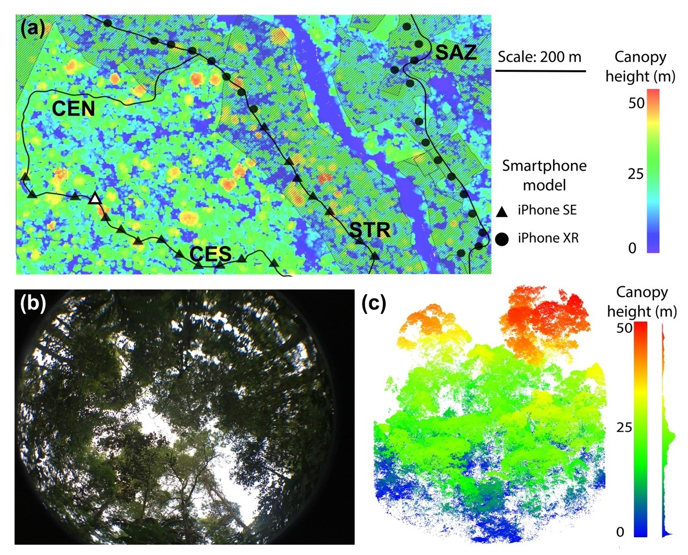
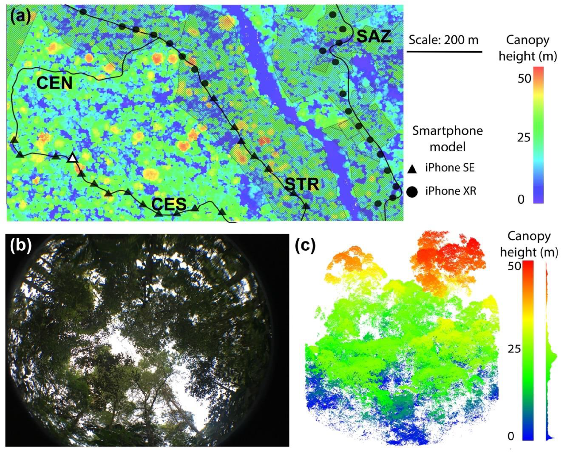
2.1. Study Area

Our study area was La Selva Biological Station, situated within an intact lowland tropical forest of northeastern Costa Rica at 10°26′ N and 83°59′ W. The mean annual temperature is 26 °C and the mean annual rainfall is 4000 mm [24]. Average daytime temperature remains fairly constant year-round while the months of January through April and September and October see drier conditions—however, even during the drier period, monthly total rainfall rarely fails to exceed 100 mm [25]. La Selva’s forests are multilayered and biodiverse, containing species of trees, lianas, epiphytes and broad-leafed monocots; the leguminous tree species Pentaclethra macroloba is particularly abundant in old growth regions [25]. The station includes a mixture of evergreen old growth and secondary tropical wet forest and our data was acquired from both forest age classes (Figure 1a). The CES trail along with portions of the CEN trail traverse old terrace primary forest. In addition to Pentaclethra, the upper canopy in this forest type is characterized by large emergent such as Dipteryx panamensis and Hymenolobium mesoamericanum (both members of Fabaceae), the subcanopy is abundant in Warscewiczia coccinea (Rubiaceae) and the understory is dominated by Capparis pittieri (Caparaceae) and the palm Bactris porschiana. Secondary forest, which encompasses most of the STR and SAZ trail locations included here, is dominated by tree species such as Cecropia insignis and C. obtusifolia (both Cecropiaceae), Goethalsia meiantha (Tiliaceae) and Laetia procera (Flacourtiaceae) [25].

2.2. Lidar Data Acquisition and PAI_eff Calculation

Airborne lidar data were collected using the Brown Platform for Autonomous Remote Sensing (BPAR) 10–14 May 2019. BPAR uses a gasoline powered helicopter-style drone platform (designed and operated by Aeroscout GmbH) and includes a Riegl VUX-1 lidar scanner and an Oxford Technical Solutions (OXTS) Survey + 2 GPS-IMU [26]. Lidar data from BPAR have a location error <5 cm; this and other characteristics of BPAR are provided in Kellner et al. (2019), which describes data collected by this platform with analogous flight design at a different location [26]. For this study, we used lidar data collected over ~1 km² of forest (Figure 1). Lidar were collected from the BPAR using two sets of orthogonal flight lines 90 m above the canopy (yielding footprint size ~5 cm at canopy level), with flight speed of 6 m/s. Parallel flight lights were 25 m apart, resulting in ~90% overlap between lines. Each lidar beam had up to 6 returns, resulting in an average total point density of ~3500 pts m⁻². Lidar data were projected in UTM 16N, WGS 1984 ellipsoidal format; we converted lidar returns heights from absolute height to height above ground using an existing lidar-derived digital terrain model (DTM) validated using 4184 independent measurements of ground height (intercept = −0.406, slope = 0.999, r² = 0.994, RMSE = 1.85 m) [27].

We computed vertical PAI_eff profiles from our discrete return lidar cloud point using the algorithm derived by Detto et al. (2015) which is based on stochastic radiative transfer theory [13]. This algorithm estimates leaf area in vertical layers using information about light (lidar beam) interception based on the height, return number and scan angle of lidar returns in an area. PAI_eff is estimated based on an assumed leaf angle distribution (LAD; “spherical”, “planophile”, “erectophile” or user-defined). We calculated PAI_eff profiles using lidar returns with x- and y-coordinates within a given radius around fisheye image locations (Figure 1). Initially, the radius was calculated as the mean forest canopy height, 20 m, times $\sqrt{3}$ because the field of view of the fisheye lens used to capture the smartphone images was 60°. Because the algorithm of Detto et al. (2015) does not use information about the horizontal path of lidar beams (i.e., beams passing into or out of the area of interest) we excluded lidar returns with a scan angle greater than 5°, resulting in average point density of 316 pts m⁻² used for PAI_eff estimation (range 291–347 pts m⁻²) [13]. Every lidar sample used to estimate PAI_eff in this study included >90,000 pts, well above the density needed to reduce relative bias and error to <5% in a vertically in-homogenous canopy, as demonstrated by Detto et al. with simulated point cloud data [13]. We calculated PAI_eff profiles in 1-m vertical bins from 1 to 60 m in height; we summed PAI_eff across all vertical layers to calculate total PAI_eff. We will refer to PAI_eff estimated using drone based discrete return lidar data as “lidar PAI_eff”.

2.3. Hemispherical Image Acquisition and PAI_eff Calculation

Ground based smartphone images were taken along four established trails within the La Selva research forest. We attached a clip-on fisheye camera lens (Criacr AMIR fisheye lens) to an Apple iPhone SE or iPhone XR mounted on a tripod stand so that our images were acquired from 1 m above the ground surface (the purpose of our study was not to compare phone models but fieldwork constraints necessitated the use of different phones). Images were taken over the time period from 15 May to 22 May in 2019. Images were taken every 50 m at previously geo-referenced trail markers along the STR, SAZ, CES and CEN trails (Figure 1). Trail markers were geo-referenced using a Garmin GPSMAP^® 60CSx unit in 2005. Of the 22 images acquired by the iPhone XR, 1 was taken in the old growth forest type and 21 were taken in the secondary growth forest type. Of the 20 images acquired by the iPhone SE, 13 were taken in the old growth forest type and 7 were taken in the secondary growth forest type. In total, we took 14 hemispherical photos of old growth canopy and 28 hemispherical photos of secondary growth canopy. We attached a bubble level to each phone to ensure that the camera was flat when images were taken, and we used a compass to ensure that images were taken using a consistent orientation. All images were taken under diffuse light conditions at dawn. Both the iPhone SE and the iPhone XR have a single 12-megapixel wide camera with an f/1.8 aperture and an optical image stabilization feature. Camera settings were set to the default modes and neither flash photography nor digital zoom were used during image acquisition. The pixel radius for 60° field of view was 1580. We will refer to PAI_eff estimated using smartphone fisheye images as “smartphone PAI_eff”.

Smartphone PAI_eff was calculated from fisheye images using CAN-EYE (v6.495), a freely available Windows imaging software developed by the French National Institute of Agricultural Research to extract canopy structure characteristics from true-color hemispherical images [28]. CAN-EYE accepts inputs of digital hemispherical images and applies a user interactive segmentation process that classifies pixels as either vegetation or non-vegetation to create a binarized image from which gap fraction is derived. Random error introduced by operator subjectivity is not completely avoidable but all images were processed in CAN-EYE by the same user to avoid issues of subjectivity between users. Optical distortions were carefully classified in the same manner for each photo and an example classification is shown in Figure S1. The classification guidelines established in Figure S1 were followed for all subsequent image processing. Images were limited to a 60° field of view to exclude distorted mixed pixels occurring at the image edges. CAN-EYE computes the gap fraction using the Poisson model and corrects for leaf clumping by computing a clumping index using the Lang and Yueqin (1986) logarithm gap fraction averaging method, which assumes vegetation elements are locally randomly distributed [29]. CAN-EYE includes multiple methods to estimate PAI_eff but we used the method based on LAI-2000 measurements in which the ring angular response is taken into account. The computation can be made using 3, 4 or 5 rings, which corresponds to the number of directional measurements used in the calculation [30]. We carried out our initial PAI_eff estimations using all three ring methods, which we call smartphone PAI3, PAI4 and PAI5, respectively. The CAN-EYE user manual includes detailed explanations of the computations and models used for image processing and PAI_eff estimation.

CAN-EYE requires a manual calibration of the optical center of the fisheye lens. We used a simple calibration method proposed in the user manual to determine an optical center of (1487, 2113) (see Section 6.2 of the CAN-EYE user manual) [28]. The position of the lens was carefully marked on both smartphones during the image acquisition process to reduce error that might be introduced into the optical center calibration by reattaching the lens in the wrong position. We assumed a perfect optical system and used a linear projection model. The impact of this assumption on results is small considering other components of measurement uncertainty. See

Table 1. General parameter inputs for CAN-EYE image processing. See the CAN-EYE user manual for detailed descriptions of each parameter [28].

Zenith Angular Resolution	2.5°	Azimuth Angular Resolution	2.5°
Circle of Interest	60°	PAISat for clumping	8
Integration domain for fCover (°)	0–10°	SubSampling Factor	1

for other general parameters used in CAN-EYE PAI_eff computation.

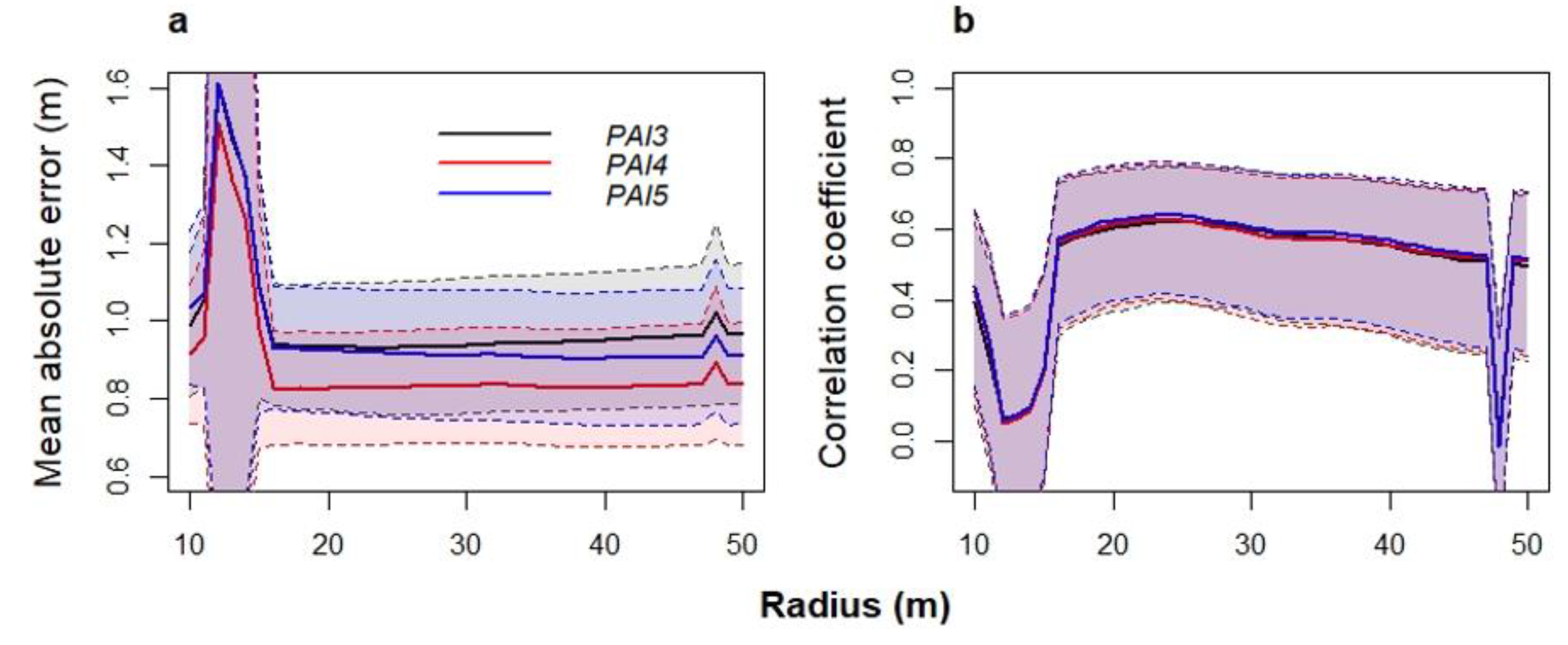
2.4. Optimization of Lidar Sample Radius

Smartphone images and lidar data were obtained within two weeks of each other to reduce any seasonal or stochastic foliage changes between our two datasets. We performed all calculations comparing lidar and smartphone PAI_eff values in R version 3.5.2 [31]. We first examined the overlapping regions of our image locations and the spatial extent of the lidar data to determine that 42 hemispherical images lay within the range of available lidar data.

To compare lidar and smartphone PAI_eff, we determined the spatial extent of smartphone images and identified all lidar data in each image. We will refer to this classification as our close points calculation. The mean canopy height of our study forest is 20.3 ± 6.9 m [32] and the field of view of our fisheye lens is 60°. From this information, we determined the projected mean radius of smartphone images to be 35 m. However, to test the effects of altering the radius in our close points calculation on the strength of the PAI_eff comparison, we calculated close points for each image location over a range of radii from 10m to 50m in 1m increments. To compare the concordance between lidar and smartphone PAI_eff for each radius, we determined the mean absolute error (MAE) and Pearson’s correlation coefficient (r) between PAI_eff estimates from each method. For this initial assessment, we assumed a spherical LAD option in the lidar PAI_eff algorithm. For subsequent analyses, we used the radius that gave the highest correlation and lowest MAE. PAI_eff data, including all three smartphone PAI_eff estimates, x and y coordinates for each trail location, forest type, phone model, and lidar PAI_eff estimates using the optimized radius and all three LADs, are available for all 42 trail locations in the Supplement (File S1).

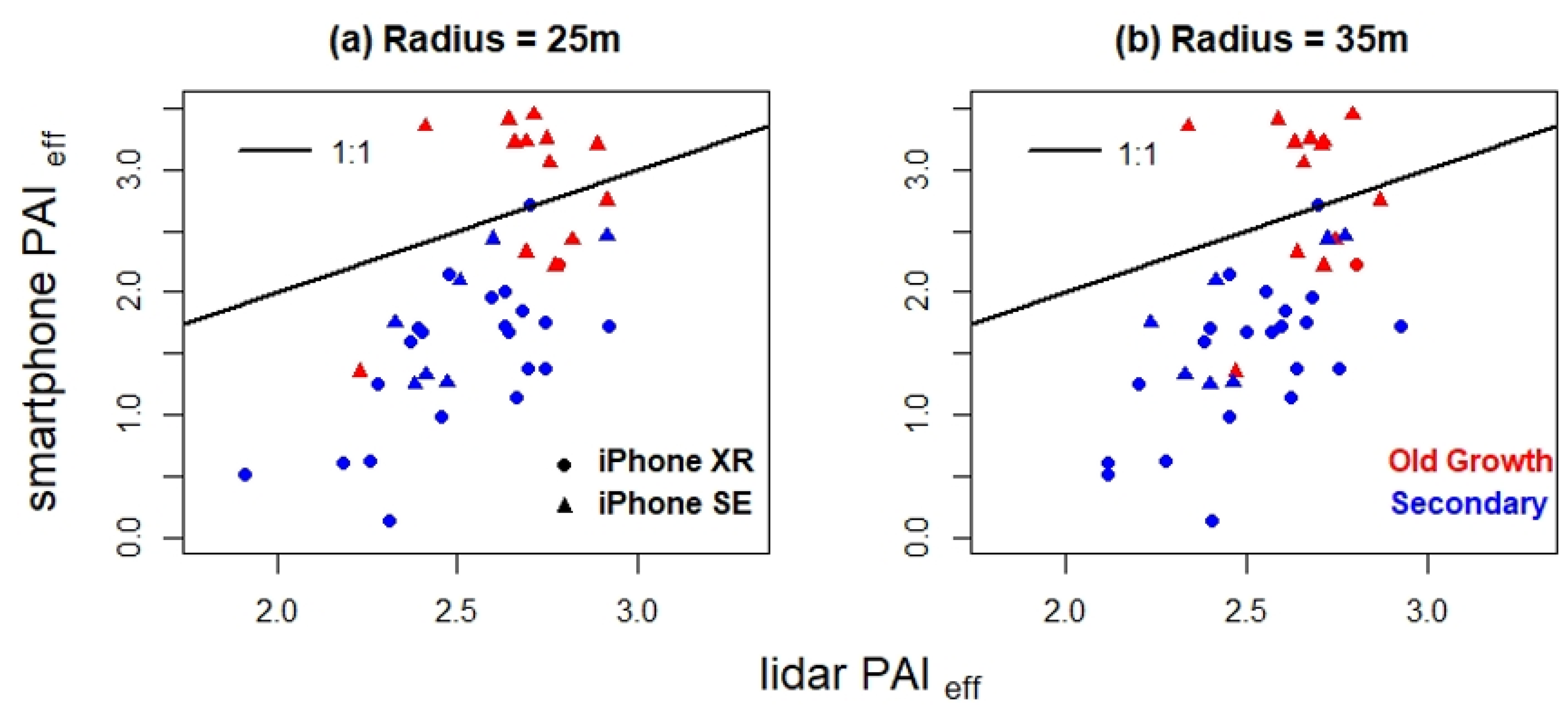
2.5. Comparing Old Growth and Secondary Forests

Our study area encompasses old growth and secondary forest, so we examined if PAI_eff estimation methods varied in concordance between the two different forest types. We compared correlation values, MAE and mean signed error (MSE) between lidar and smartphone PAI_eff estimates for the subsets of old growth and secondary growth forests using all LAD options in the lidar PAI_eff algorithm (spherical, erectophile and planophile). For subsequent analyses, we used the LAD for each forest type that resulted in the highest correlation and lowest MAE for that forest type.

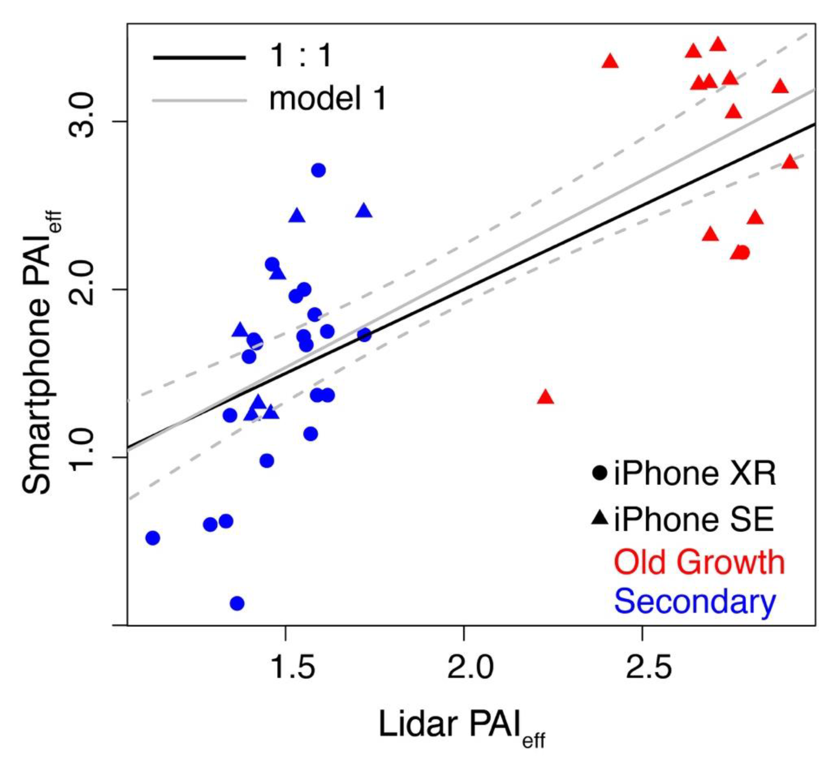
2.6. Final Comparison of Lidar and Smartphone PAI_eff

Our final comparison of lidar and smartphone PAI_eff used the optimal lidar radius and LADs determined above. Additionally, we tested for residual bias caused by differences between smartphone models and unaccounted for difference between old growth and secondary forests by comparing four linear models:

• Model 1: Smartphone PAI_eff ~ Lidar PAI_eff
• Model 2: Smartphone PAI_eff ~ Lidar PAI_eff + Phone model
• Model 3: Smartphone PAI_eff ~ Lidar PAI_eff + Forest type
• Model 4: Smartphone PAI_eff ~ Lidar PAI_eff + Phone model + Forest type

We compared the AIC values of these models. If models 2–4 outperformed model 1 (ΔAIC > 2), we considered there to be evidence that there is significant residual variation in smartphone PAI_eff (after considering real differences in forest structure as measured by lidar PAI_eff) that is explained by phone model and/or forest type.

3. Results

3.1. Correlation and MAE as a Function of Lidar Radius

The initial maximum correlation between smartphone and lidar PAI_eff was r = 0.64 and occurred at a lidar radius of 25 m using image method PAI5 (DF = 40, p < 0.001; Figure 2 and Figure 3); however, we found very little difference in correlation values between the three image methods (PAI3, PAI4 and PAI5) across most of the considered range in radii. MAE and correlation values calculated for each method varied together and gradually over most of the range of radii tested (Figure 2). The gradual change in MAE and correlation broke down at radii less than 16m and greater than 47 m. We suspect this is due to the spatial structure of the forest canopy not being consistent at radii extremely smaller or larger than the radii of the smartphone images. There were larger differences between the smartphone PAI_eff methods in MAE than in correlation values. The three-ring method (PAI3) consistently introduced the highest MAE while the four-ring method (PAI4) introduced the lowest; however, correlation values were more similar across the three methods. PAI_eff estimates with each method were highly correlated (Figure S2), so all subsequent analyses were conducted using the PAI4 method to reduce MAE.

3.2. Differences in Old Growth versus Secondary Growth Forest

The highest concordance between smartphone and lidar PAI_eff in old growth and secondary forest was found using LADs in the lidar PAI_eff calculation that varied by forest type—for old growth locations, mean absolute error (MAE) between smartphone and lidar PAI_eff was more than twice as large when using a planophile LAD in the lidar PAI_eff calculation than when using a spherical or erectophile LAD; however, for secondary forest locations, MAE was more than twice as large when using a spherical LAD than a planophile or erectophile LAD (

Table 2. Mean absolute error (MAE), mean signed error (MSE), Pearson’s correlation coefficient (r), 95% confidence intervals (CI) for r and mean PAI_eff values comparing lidar and smartphone PAI_eff in subsets of old growth (n = 14) and secondary forest (n = 28) locations. Lidar PAI_eff was estimated using radius = 25 m and spherical (S), planophile (P) and erectophile (E) leaf angle distributions (LADs). * denotes statistically significant values (p < 0.05).

Forest Type	LAD	MAE	MSE	r	95% CI	Mean Smartphone PAIeff	Mean Lidar PAIeff
Old Growth	P	1.228	−1.228	0.306	[−0.268, 0.720]	2.816	1.588
Secondary	P	0.426	−0.057	0.637 *	[0.346, 0.816]	1.538	1.481
Old Growth	S	0.542	−0.124	0.306	[−0.268, 0.720]	2.816	2.693
Secondary	S	0.973	0.972	0.637 *	[0.346, 0.816]	1.538	2.510
Old Growth	E	0.531	0.354	0.306	[−0.26, 0.720]	2.816	3.170
Secondary	E	1.417	1.417	0.637 *	[0.346, 0.816]	1.538	2.955

). Similarly, for old growth locations, mean signed error (MSE) was minimized when a spherical LAD was used while for secondary forest locations, MSE was minimized when a planophile LAD was used. The Pearson’s correlation values were higher for secondary forest locations (r = 0.64, DF = 26, p < 0.001) than for old growth forest locations (r = 0.31, DF = 12, p = 0.287) and the 95% confidence interval of the old growth correlation value overlapped with zero. Using the optimal LAD for each forest type, the mean signed error (MSE) was negative for both old growth and secondary forest types, indicating that smartphone PAI_eff was greater than lidar PAI_eff. The magnitude of MSE was greater for old growth forests (−0.124) than for secondary forests (−0.057) (

Table 3. Comparison among models to explain variation in smartphone PAI_eff. All models were fit using all 42 observations of smartphone and lidar PAI_eff at La Selva. All ΔAIC values are relative to model 1. Values for r² are the adjusted r² values for each linear model.

Model	ΔAIC	p	r2
1: Smartphone PAIeff ~ Lidar PAIeff	0.00	<0.001	0.59
2: Smartphone PAIeff ~ Lidar PAIeff + Phone model	−0.18	<0.001	0.60
3: Smartphone PAIeff ~ Lidar PAIeff + Forest type	−0.97	<0.001	0.61
4: Smartphone PAIeff ~ Lidar PAIeff + Phone model + Forest type	−3.00	<0.001	0.63

).

3.3. Final Comparison of Lidar and Smartphone PAI_eff

Using the optimal lidar radius and forest type LADs described above, we found a very significant correlation between smartphone and lidar PAI_eff (r = 0.77, DF = 40, p < 0.001; Figure 4). We used a model comparison framework to evaluate whether significant residual variation was explained by phone model and/or forest type (Table 3). We found that only the model including effects of both phone model and forest type (model 4) was significantly better than the original model (i.e., had ΔAIC < 2). However, model 4 explained only 4% more variation than model 1, indicating that while bias due to smartphone model and forest type was significant, its total magnitude was small (Table 3).

4. Discussion

We found that smartphone based PAI_eff estimates using an inexpensive (<$20) clip-on fisheye lens were significantly correlated with PAI_eff estimates from high density drone based lidar (Figure 4). Further, the strength of this correlation was robust to choices of image processing options (Figure 2) and the model of smartphone used (Table 3). Our results indicate that inexpensive smartphone methods are valid for characterizing relative spatial variation in PAI_eff within a tropical forest canopy.

While we are confident that our lidar method is appropriate for estimating spatial variability in PAI_eff, without destructive measurements of leaf area we cannot know if the magnitude of lidar PAI_eff is itself biased. Both lidar and smartphone PAI_eff estimates in this study are smaller than those reported previously from DHP (3.76 ± 0.11 SE) for 18 0.5 ha plots in the old growth forest at La Selva [10] but our measurements were taken following an unprecedented blowdown disturbance that caused widespread mortality at La Selva in May 2019, so our lower PAI_eff values may be realistic [33].

Our results are consistent with those of Wang et al. (2018), who also found that smartphone based methods are appropriate for comparing trends in leaf area—they found r² values of 0.706 when they compared fisheye lens PAI_eff to LAI-2200 and 0.695 when compared to MODIS satellite data in a pine tree plantation forest [23]. It is meaningful that our data align with these results because we show that an inexpensive fisheye lens PAI_eff estimation method can be effective in a spatially complex and heterogeneous tropical forest, in addition to relatively homogeneous plantation canopies examined in Wang et al. (2018) [23]. Our correlation values were somewhat less strong (r² = 0.59) than this previous study. This is expected because we are comparing ground based LAI_eff estimates (smartphone LAI_eff) to airborne LAI_eff estimates (lidar LAI_eff). Sensors beneath and above the canopy view the forest differently—trunks are prominent in ground-based images (Figure 1b) while a previous study found that non-photosynthetic material accounts for only 7% of reflected radiation (i.e., lidar returns) in this landscape [17]. We believe that finding significant correlation between two approaches to estimate PAI_eff with different views and analytical methods (smartphone images are passive 2D data while lidar points are active 3D data) shows strong support that smartphones can describe spatial variation in PAI_eff. This result builds off the conclusions of Olivas et al. (2013), who suggested that applying leaf clumping corrections to DHPs led to the most efficient estimation method of landscape level PAI_eff estimation and characterization in a tropical forest [22]. We extend this conclusion to show that fisheye images collected by smartphones can be used as a more inexpensive yet still efficient method of estimating PAI_eff spatial variation in a tropical forest.

The strength of our correlation between smartphone and lidar PAI_eff is also somewhat smaller than correlations previously reported by studies comparing LAI estimated with true DHP to LAI estimated using airborne lidar. These studies—all from temperate regions—report r² values between 0.72 and 0.86 [16,34,35]. We acknowledge two additional sources of error that could cause the relationship between smartphone and lidar PAI_eff to be weaker in our study compared to previous analyses. First, PAI_eff estimations derived from smartphone images are likely affected by random and systematic errors introduced by the image processing chains raw data undergo before becoming available to the user. Second, there may be geo-referencing errors between the smartphone and data because trail marker locations were geo-located using a handheld GPS unit.

We found that the strength of correlation between smartphone and lidar PAI_eff increased substantially when using forest-type specific LADs in the lidar PAI_eff algorithm (Figure 3 and Figure 4). Specifically, we found that a spherical LAD was best for old growth forest while a planophile LAD was best for secondary forest (Table 2). We believe that this result is ecologically appropriate because many common pioneer trees in Neotropical forests, such as Cecropia, have leaves that are much flatter than predicted by a spherical distribution [36]. MSE was close to zero for secondary growth locations when a planophile LAD was used for the lidar PAI_eff calculation, suggesting no directional systematic bias between smartphone and lidar PAI_eff calculation methods in secondary forests. As expected, both smartphone and lidar PAI_eff found that total PAI_eff was higher in old growth than secondary forests but we found a higher correlation within secondary forest areas compared to old growth forest areas (Table 2). We cannot know with certainty which method is more accurate without doing destructive sampling to directly measure PAI_eff but we suspect that the passive hemispherical image method may perform worse in dense vegetation. Using simulations, the active lidar method was found to perform well at our sample sizes for a range of PAI_eff values [13].

It is important to note that we found small (4%) but significant, residual bias explained by a combination of phone model and forest type (Table 3). Neither phone model nor forest type alone explained significant residual bias. However, our sampling design was not intended to test for differences between phone models—the use of two phones in this study was necessitated by the reality of fieldwork. Future studies could more thoroughly characterize the influence of smartphone camera characteristics on smartphone PAI_eff in different forest types.

5. Conclusions

Our data reveals that inexpensive, smartphone fisheye images can be used to reasonably compare spatial variation in PAI_eff in a heterogeneous tropical forest canopy. This method offers an extremely inexpensive and efficient alternative to estimating PAI_eff using more complicated and expensive equipment, overcoming the obstacle of price that can be prohibitive to conducting studies of PAI_eff variation. However, absolute differences in smartphone PAI_eff and lidar PAI_eff vary across parameters (radius, leaf angle distribution, photo method, smartphone model), suggesting that other information may be necessary to measure the absolute magnitude of PAI_eff. It may be possible to further explain the remaining variation in the relationship between smartphone and lidar estimates by considering reliable measurements of other canopy structural properties (e.g., canopy gap fractions) or by comparing to direct harvest LAI measurements.

References

1. Clark, D.A.; Asao, S.; Fisher, R.; Reed, S.; Reich, P.B.; Ryan, M.G.; Wood, T.E.; Yang, X. Reviews and Syntheses: Field Data to Benchmark the Carbon Cycle Models for Tropical Forests. Biogeosciences 2017, 14, 4663–4690. [Google Scholar] [CrossRef] [Green Version]
2. Doughty, C.E.; Goulden, M.L. Seasonal Patterns of Tropical Forest Leaf Area Index and CO2 Exchange. J. Geophys. Res. Biogeosci. 2009, 114, 1–12. [Google Scholar] [CrossRef] [Green Version]
3. Herbert, D.A.; Fownes, J.H. Phosphorus Limitation of Forest Leaf Area and Net Primary Production on a Highly Weathered Soil. Biogeochemistry 1995, 29, 223–235. [Google Scholar] [CrossRef]
4. Stark, S.C.; Enquist, B.J.; Saleska, S.R.; Leitold, V.; Schietti, J.; Longo, M.; Alves, L.F.; Camargo, P.B.; Oliveira, R.C. Linking Canopy Leaf Area and Light Environments with Tree Size Distributions to Explain Amazon Forest Demography. Ecol. Lett. 2015, 18, 636–645. [Google Scholar] [CrossRef]
5. Tang, H.; Dubayah, R. Light-Driven Growth in Amazon Evergreen Forests Explained by Seasonal Variations of Vertical Canopy Structure. Proc. Natl. Acad. Sci. USA 2017, 114, 2640–2644. [Google Scholar] [CrossRef] [Green Version]
6. Watson, D.J. Comparative Physiological Studies on the Growth of Field Crops: I. Variation in Net Assimilation Rate and Leaf Area between Species and Varieties, and within and between Years. Ann. Bot. 1947, 11, 41–76. [Google Scholar] [CrossRef]
7. Asner, G.P.; Scurlock, J.M.O.; Hicke, J.A. Global Synthesis of Leaf Area Index Observations: Implications for Ecological and Remote Sensing Studies. Glob. Ecol. Biogeogr. 2003, 12, 191–205. [Google Scholar] [CrossRef] [Green Version]
8. Clark, D.B.; Olivas, P.C.; Oberbauer, S.F.; Clark, D.A.; Ryan, M.G. First Direct Landscape-Scale Measurement of Tropical Rain Forest Leaf Area Index, a Key Driver of Global Primary Productivity. Ecol. Lett. 2008, 11, 163–172. [Google Scholar] [CrossRef]
9. Liu, Z.; Chen, J.M.; Jin, G.; Qi, Y. Estimating Seasonal Variations of Leaf Area Index Using Litterfall Collection and Optical Methods in Four Mixed Evergreen-Deciduous Forests. Agric. For. Meteorol. 2015, 209–210, 36–48. [Google Scholar] [CrossRef]
10. Loescher, H.W.; Oberbauer, S.F.; Gholz, H.L.; Clark, D.B. Environmental Controls on Net Ecosystem-Level Carbon Exchange and Productivity in a Central American Tropical Wet Forest. Glob. Chang. Biol. 2003, 9, 396–412. [Google Scholar] [CrossRef]
11. Cutini, A.; Matteucci, G.; Mugnozza, G.S. Estimation of Leaf Area Index with the Li-Cor LAI 2000 in Deciduous Forests. For. Ecol. Manag. 1998, 105, 55–65. [Google Scholar] [CrossRef]
12. Jupp, D.L.B.; Culvenor, D.S.; Lovell, J.L.; Newnham, G.J.; Strahler, A.H.; Woodcock, C.E. Estimating Forest LAI Profiles and Structural Parameters Using a Ground-Based Laser Called Echidna®. Tree Physiol. 2009, 29, 171–181. [Google Scholar] [CrossRef] [PubMed]
13. Detto, M.; Asner, G.P.; Muller-Landau, H.C.; Sonnentag, O. Spatial Variability in Tropical Forest Leaf Area Density from Multireturn Lidar and Modeling. J. Geophys. Res. Biogeosci. 2015, 120, 294–309. [Google Scholar] [CrossRef]
14. Tang, H.; Dubayah, R.; Brolly, M.; Ganguly, S.; Zhang, G. Large-Scale Retrieval of Leaf Area Index and Vertical Foliage Profile from the Spaceborne Waveform Lidar (GLAS/ICESat). Remote Sens. Environ. 2014, 154, 8–18. [Google Scholar] [CrossRef]
15. Bréda, N.J.J. Ground-Based Measurements of Leaf Area Index: A Review of Methods, Instruments and Current Controversies. J. Exp. Bot. 2003, 54, 2403–2417. [Google Scholar] [CrossRef] [PubMed]
16. Tang, H.; Brolly, M.; Zhao, F.; Strahler, A.H.; Schaaf, C.L.; Ganguly, S.; Zhang, G.; Dubayah, R. Deriving and Validating Leaf Area Index (LAI) at Multiple Spatial Scales through Lidar Remote Sensing: A Case Study in Sierra National Forest, CA. Remote Sens. Environ. 2014, 143, 131–141. [Google Scholar] [CrossRef]
17. Tang, H.; Dubayah, R.; Swatantran, A.; Hofton, M.; Sheldon, S.; Clark, D.B.; Blair, B. Retrieval of Vertical LAI Profiles over Tropical Rain Forests Using Waveform Lidar at La Selva, Costa Rica. Remote Sens. Environ. 2012, 124, 242–250. [Google Scholar] [CrossRef]
18. Calders, K.; Origo, N.; Disney, M.; Nightingale, J.; Woodgate, W.; Armston, J.; Lewis, P. Variability and Bias in Active and Passive Ground-Based Measurements of Effective Plant, Wood and Leaf Area Index. Agric. For. Meteorol. 2018, 252, 231–240. [Google Scholar] [CrossRef]
19. Leblanc, S.G.; Chen, J.M.; Fernandes, R.; Deering, D.W.; Conley, A. Methodology Comparison for Canopy Structure Parameters Extraction from Digital Hemispherical Photography in Boreal Forests. Agric. For. Meteorol. 2005, 129, 187–207. [Google Scholar] [CrossRef] [Green Version]
20. Chen, J.M. Optically-Based Methods for Measuring Seasonal Variation of Leaf Area Index in Boreal Conifer Stands. Agric. For. Meteorol. 1996, 80, 135–163. [Google Scholar] [CrossRef]
21. Chen, J.M.; Cihlar, J. Plant Canopy Gap-Size Analysis Theory for Improving Optical Measurements of Leaf-Area Index. Appl. Opt. 1995, 34, 6211. [Google Scholar] [CrossRef] [PubMed] [Green Version]
22. Olivas, P.C.; Oberbauer, S.F.; Clark, D.B.; Clark, D.A.; Ryan, M.G.; O’Brien, J.J.; Ordoñez, H. Comparison of Direct and Indirect Methods for Assessing Leaf Area Index across a Tropical Rain Forest Landscape. Agric. For. Meteorol. 2013, 177, 110–116. [Google Scholar] [CrossRef]
23. Wang, J.X.; Xiong, Q.C.; Lin, Q.N.; Huang, H.G. Feasibility of Using Mobile Phone to Estimate Forest Leaf Area Index: A Case Study in Yunnan Pine. Remote Sens. Lett. 2018, 9, 180–188. [Google Scholar] [CrossRef] [Green Version]
24. Sanford, R.L., Jr.; Paaby, P.; Luvall, J.C.; Phillips, E. Climate, geomorphology, and aquatic systems. In La Selva: Ecology and Natural History of a Neotropical Rain Forest; McDade, L.A., Bawa, K.S., Hespenheide, H.A., Hartshorn, G.S., Eds.; University of Chicago Press: Chicago, IL, USA, 1994; pp. 19–33. [Google Scholar]
25. Hartshorn, G.S.; Hammel, B.E. Vegetation types and floristic patterns. In La Selca: Ecology and Natural History of a Neotropical Rain Forest; McDade, L.A., Bawa, K.S., Hespenheide, H.A., Hartshorn, G.S., Eds.; University of Chicago Press: Chicago, IL, USA, 1994; pp. 73–89. [Google Scholar]
26. Kellner, J.R.; Armston, J.; Birrer, M.; Cushman, K.C.; Duncanson, L.; Eck, C.; Falleger, C.; Imbach, B.; Král, K.; Krůček, M.; et al. New Opportunities for Forest Remote Sensing through Ultra-High-Density Drone Lidar. Surv. Geophys. 2019, 40, 959–977. [Google Scholar] [CrossRef] [PubMed] [Green Version]
27. Kellner, J.R.; Clark, D.B.; Hofton, M.A. Canopy Height and Ground Elevation in a Mixed-Land-Use Lowland Neotropical Rain Forest Landscape. Ecology 2009, 90, 3274. [Google Scholar] [CrossRef] [Green Version]
28. Weiss, M.; Baret, F. Can-Eye V6.4.91 User Manual. Available online: https://www6.paca.inrae.fr/can-eye/content/download/3052/30819/version/4/file/CAN_EYE_User_Manual.pdf (accessed on 2 January 2020).
29. Lang, A.R.G.; Yueqin, X. Estimation of Leaf Area Index from Transmission of Direct Sunlight in Discontinuous Canopies. Agric. For. Meteorol. 1986, 37, 229–243. [Google Scholar] [CrossRef]
30. Weiss, M.; Baret, F.; Smith, G.J.; Jonckheere, I.; Coppin, P. Review of Methods for in Situ Leaf Area Index (LAI) Determination Part II. Estimation of LAI, Errors and Sampling. Agric. For. Meteorol. 2004, 121, 37–53. [Google Scholar] [CrossRef]
31. R Core Team. R: A Language and Environment for Statistical Computing; R Foundation for Statistical Computing: Vienna, Austria, 2018; URL; Available online: https://www.R-project.org/ (accessed on 8 January 2020).
32. Kellner, J.R.; Clark, D.B.; Hubbell, S.P. Pervasive Canopy Dynamics Produce Short-Term Stability in a Tropical Rain Forest Landscape. Ecol. Lett. 2009, 12, 155–164. [Google Scholar] [CrossRef]
33. Rader, A.M.; Cottrell, A.; Kudla, A.; Lum, T.; Henderson, D.; Karandikar, H.; Letcher, S.G. Tree functional traits as predictors of microburst-associated treefalls in tropical wet forests. Biotropica 2020, 52, 410–414. [Google Scholar] [CrossRef]
34. Kamoske, A.G.; Dahlin, K.M.; Stark, S.C.; Serbin, S.P. Leaf area density from airborne LiDAR: Comparing sensors and resolutions in a temperate broadleaf forest ecosystem. For. Ecol. Manag. 2019, 433, 364–375. [Google Scholar] [CrossRef]
35. Kamoske, A.G. Personal Communication; Michigan State University: East Lansing, MI, USA, 2020. [Google Scholar]
36. Ackerly, D.D.; Bazzaz, F.A. Seedling crown orientation and interception of diffuse radiation in tropical forest gaps. Ecology 1995, 76, 1134–1146. [Google Scholar] [CrossRef]
Figure 1. Overview of study area at La Selva, Costa Rica. (a) Lidar derived canopy height above ground. Lines show trails through the research reserve and points denote locations where smartphone images were taken. Shaded areas are secondary forests; old growth forests are unshaded. (b) Example smartphone fisheye image taken at trail location CES750 (location indicated in (a) with white triangle). (c) Example lidar point cloud data centered at trail location CES750.
Remotesensing 12 01765 g001
Figure 2. (a) Mean absolute error (MAE) and (b) Pearson’s correlation coefficient between smartphone and lidar PAIeff estimates across the 10–50 m range of radii using a spherical leaf angle distribution in the lidar PAIeff calculation. 95% confidence intervals are plotted for all three curves in (a,b). All 42 trail locations are represented in the MAE and correlation coefficient calculations, including trail location images taken by both iPhones.
Remotesensing 12 01765 g002
Figure 3. Relationship between smartphone and lidar PAIeff (using the four-ring smartphone PAIeff estimation method) assuming a spherical leaf angle distribution and using a radius of (a) 25 m and (b) 35 m in the lidar close points calculation.
Remotesensing 12 01765 g003
Figure 4. Relationship between smartphone and lidar PAIeff, using the four-ring smartphone PAIeff estimation method and optimal values for lidar radius (25 m) and leaf angle distributions (spherical for old growth, planophile for secondary). Dashed lines show the 95% confidence interval around model 1.
Remotesensing 12 01765 g004