Novel Air Temperature Measurement Using Midwave Hyperspectral Fourier Transform Infrared Imaging in the Carbon Dioxide Absorption Band

Abstract

Accurate visualization of air temperature distribution can be useful for various thermal analyses in fields such as human health and heat transfer of local area. This paper presents a novel approach to measuring air temperature from midwave hyperspectral Fourier transform infrared (FTIR) imaging in the carbon dioxide absorption band (between 4.25–4.35 $\mathsf{\mu }$m). In this study, the proposed visual air temperature (VisualAT) measurement is based on the observation that the carbon dioxide band shows zero transmissivity at short distances. Based on analysis of the radiative transfer equation in this band, only the path radiance by air temperature survives. Brightness temperature of the received radiance can provide the raw air temperature and spectral average, followed by a spatial median-mean filter that can produce final air temperature images. Experiment results tested on a database obtained by a midwave extended FTIR system (Telops, Quebec City, QC, Canada) from February to July 2018 show a mean absolute error of 1.25 ${}^{\circ }$K for temperature range of 2.6−26.4 ${}^{\circ }$C.

1. Introduction

How accurately can we measure and visualize air temperature remotely using thermal sensing? Air temperature is an important meteorological factor, which has a wide range of applications in fields like human health [1], virus propagation [2], growth and reproduction of plants [3], climate change [4], and hydrology [5].

Air temperature can be measured in numerous ways, including contact sensors and remote sensors. Contact sensor-based methods include thermistors, thermocouples, and mercury thermometers [6]. Thermistors are metallic devices that undergo predictable changes in resistance in response to changes in temperature. This resistance is measured and converted to a temperature reading in Celsius, Fahrenheit, or Kelvin. A thermocouple consists of two dissimilar electrical conductors forming an electrical junction, which produces a temperature-dependent voltage, and this voltage can be converted to a temperature [7]. A mercury thermometer consists of liquid in a glass rod with a very thin tube in it. Mercury or red-colored alcohol inside the tube expands when the temperature rises. These sensors should be located in the shade to measure air temperature. If the sun shines on the thermometer directly, it heats the liquid and produces an incorrect, higher temperature than the true air temperature. In addition, it needs enough time (at least several minutes for the liquid to expand) to measure outdoor air temperature. Furthermore, it requires hundreds of thousands contact sensors to measure spatial distribution of air temperature.

The thermal remote sensing approaches will use the relationships between land surface temperature (LST) and near surface air temperature. Land surface radiance is measured by thermal infrared sensors mounted on a satellite or an airborne platform, and LST is retrieved via temperature-emissivity separation (TES) [8,9]. Surface air temperature can be estimated by the temperature-vegetation index (TVX), thermodynamics, and the regression method. The TVX is based on the assumption that a thick vegetation canopy can approximate air temperature [10,11]. It can be useful only if there is high vegetation cover. The thermodynamics-based method uses the energy balance between LST and the surface environment, such as air and water [12,13]. This method provides good air temperature measurement, but it requires many parameters as input. The last type is data-based regression between air temperature and LST. There is a linear regression model [14] and a nonlinear model, especially as a deep learning method [15]. Such machine learning models have reported successful air temperature estimation. One recent deep learning-based method, a five-layer deep belief network (DBN), showed promising air temperature estimation by establishing the relationship between ground station air temperature and multi-source data (remote sensing radiance, socioeconomic data, and assimilation data) [15]. Although the deep learning method showed quite accurate air temperature estimation, it requires huge amounts of data to train the multi-layered deep neural architecture.

The above mentioned approaches are not suitable for instantaneously measuring and visualizing air temperature of a viewing area. Using contact sensors requires several minutes and a huge number of sensors to measure spatial air temperature [16]. Non-contact (remote) sensors, such as thermal infrared (TIR) imagers, require LST and regression with huge amounts of training data. Despite being trained correctly, the regression-based approach is sensitive to many spatio-temporal conditions [17]. In addition, this approach is only suitable for aerial-based sensing in satellites or airborne platforms [18].

In this paper, our research focuses on how to measure spatial air temperature of the viewing area and visualize it instantaneously for environment monitoring of the surveillance area. The key idea is to use up-welling information in the carbon dioxide absorption band ($4.25-$4.35 $\mathsf{\mu }$m) with a midwave Fourier transform infrared (FTIR) imager. Most temperature estimation research in TES and LST generates up-welling information by using the moderate-resolution atmospheric radiance and transmittance model (MODTRAN) for atmospheric correction (compensation) purposes [19,20,21]. Harig proposed a passive sensing of pollutant clouds by longwave FTIR to find optimal SNR [22]. His work focused on detecting cloud target in ground background not air temperature. In this paper, it is possible to measure and visualize air temperature accurately through careful analysis of upwelling (path) spectral radiance in the proposed visual air temperature (VisualAT).

The contributions from this paper can be summarized as follows. First, VisualAT can measure spatial air temperature accurately (mean absolute error [MAE]: 1.25 K). Second, VisualAT can visualize the distribution of air temperature with a high spatial resolution. Third, it can measure and visualize air temperature instantaneously. Finally, the proposed VisualAT can be used for various outdoor air temperature measurement applications, such as health monitoring, weather monitoring, and thermal surveillance of local area.

The remainder of this paper is organized as follows. Section 2 introduces the marials for FTIR analysis and Section 3 explains the proposed VisualAT method, including the radiative transfer equation. Section 4 analyzes VisualAT for temperature measurement applications, considering a range of environmental changes. The paper concludes in Section 5.

2. Materials for FTIR Analysis

2.1. Outdoor Hyperspectral Data Acquisition System

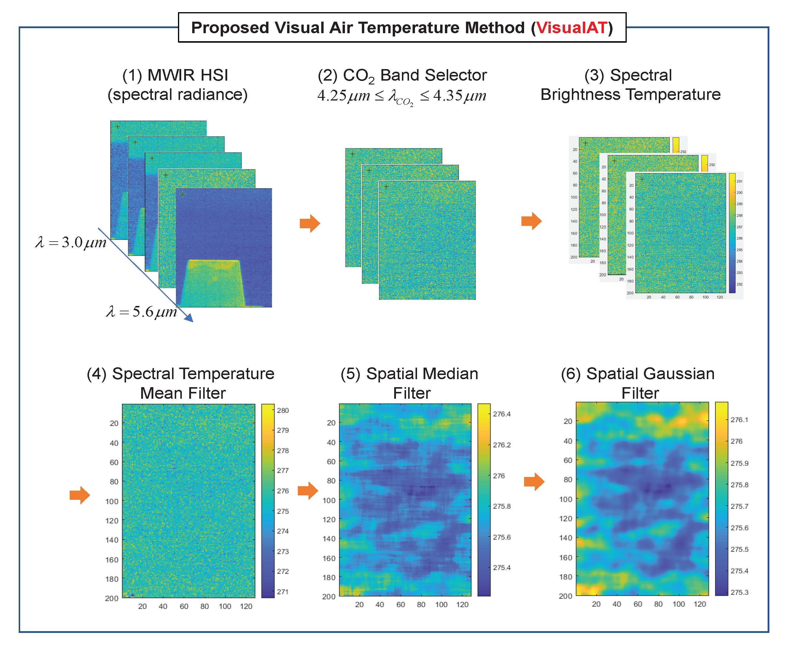
Figure 1 presents a measurement scenario in an outdoor environment consisting of a scene and a sensor system. A painted target in front of a sky-and-sea background is 78 m away from the observation laboratory. MWIR hyperspectral images were acquired with the Telops Hyper-Cam MWE model [23]. It can provide calibrated spectral radiance images with a high spatial and spectral resolution from a Michelson interferometer in the short-wave to midwave band ($1.5$–5.6 $\mathsf{\mu }$m). The spatial image resolution is $320\times 240$, and the spectral resolution is up to 0.25 cm${}^{-1}$. The noise equivalent spectral radiance (NESR) is 7 [nW/(cm${}^2·$sr· cm${}^{-1}\left)\right]$, and the radiometric accuracy is approximately 2 K. The field of view is $6.5\times 5.1$ deg.

The objective of this research is to estimate air temperature spatially and to visualize the temperature distribution. A cropped hypercube image provides $128\times 200\times 374$ (width × height × bands) data. A hyperspectral spectral imager (HSI) database was recorded daily from February to July 2018. Recording was done three times a day (10:30, 13:30, and 15:30 h) and four times an hour for a total of 12 times per day. In addition, an automatic weather station (AWS) recorded environmental information, such as the date, time, air temperature, humidity, air pressure, and visibility. The measured air temperatures were used to evaluate the temperature estimation accuracy by the proposed VisuaAT method.

2.2. FTIR Data Acquisition Interface

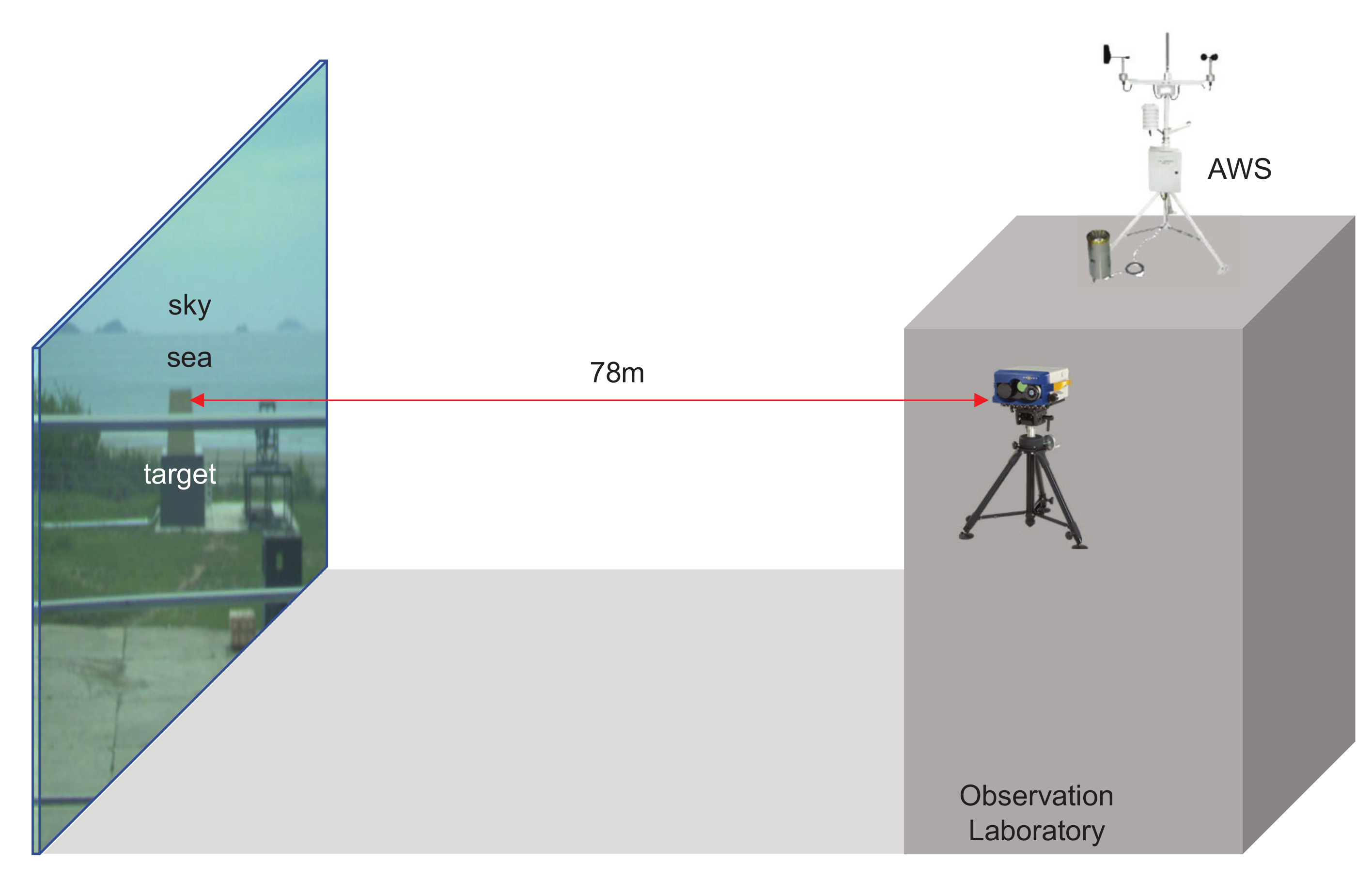
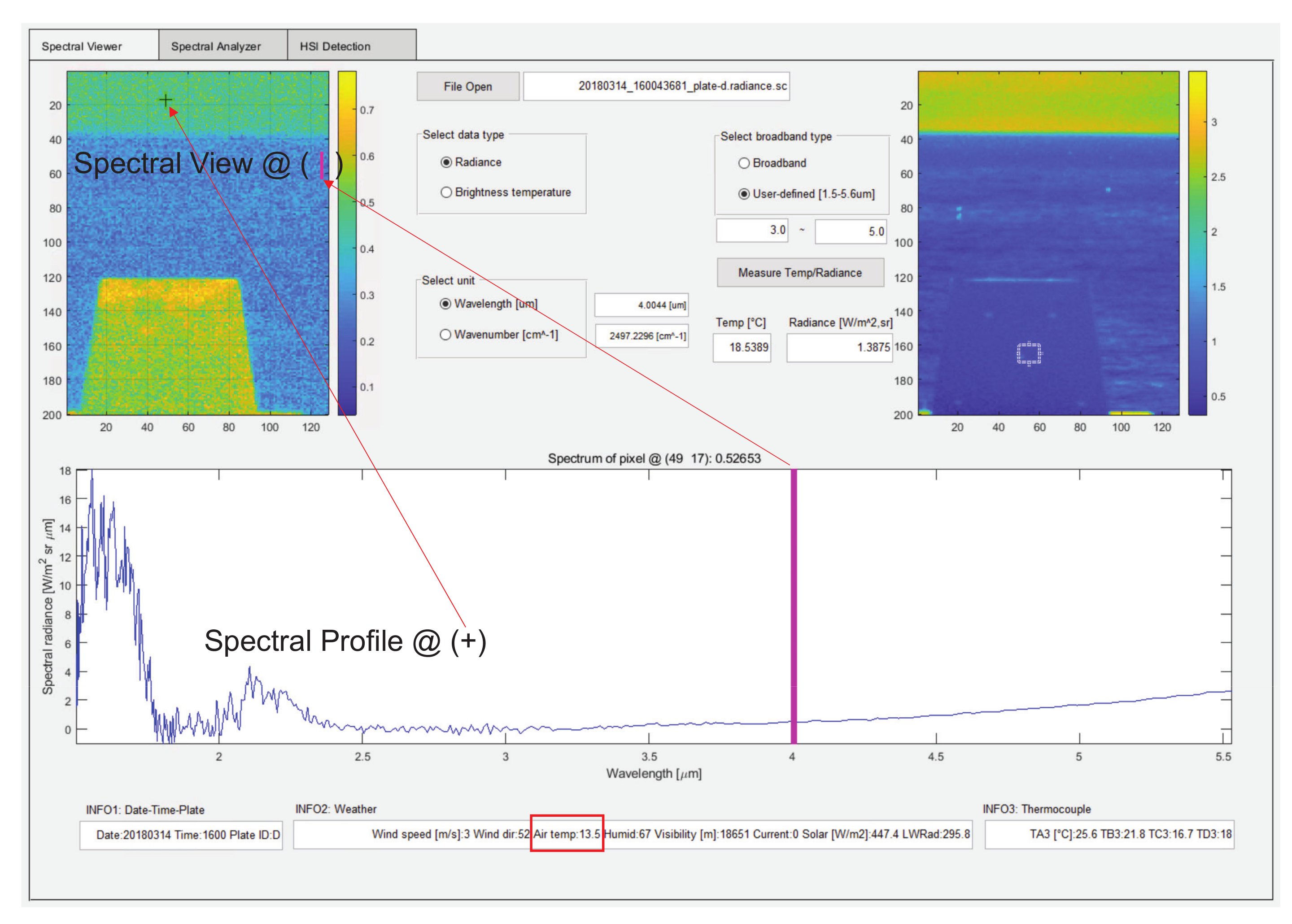
The selection of the CO${}_2$ absorption band is critical in the proposed VisualAT method. An initial baseline band range was selected by the developed GUI shown in Figure 2. The midwave FTIR spectral image software platform was developed for hypercube image display and spectral profile analysis by varying the wavelength parameter and units. The top left image in Figure 2 represents a spectral image in a specific band, and the lower graph shows a spectral profile at a selected point (indicated by +). The top right image in Figure 2 is a broad-band image with a selected spectral range.

2.3. Radiometric Calibration of FTIR Imaging

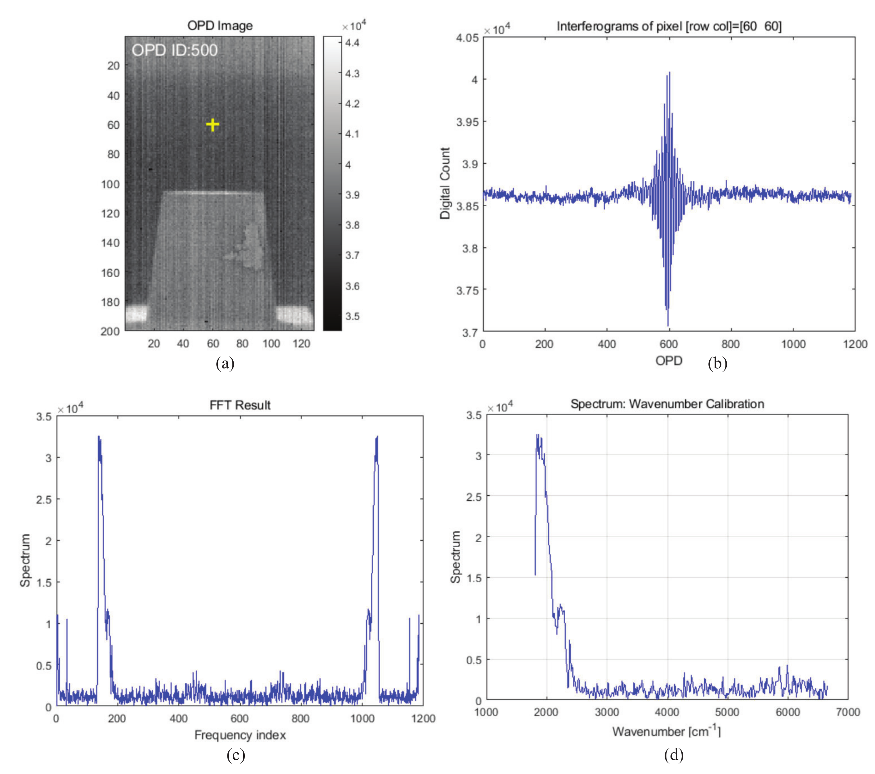
The wavenumber and radiometric calibration of midwave hyperspectral data should be done accurately to measure air temperature. The technical details are described in [24] and one full set of data including the raw IR spectrum, internal calibration, and temperature extraction is described in the following paragraphs. A Michelson interferometer produces interferomgrams by moving a mirror. Figure 3a presents an interferogram image at optical path difference (OPD) ID 500 (total 1186). Figure 3b gives an example of the whole interferogram at pixel (60, 60). Figure 3c shows the results of spectrum extraction by applying the fast Fourier transform (FFT) to the interferogram (Figure 3b). The unit of the y-$axis$ in Figure 3c is just spectral intensity in arbitrary units. The wavelength calibration is performed using the HeNe laser (wavelength $\lambda =632.8$ nm). Figure 3d shows the wavenumber calibrated spectrum.

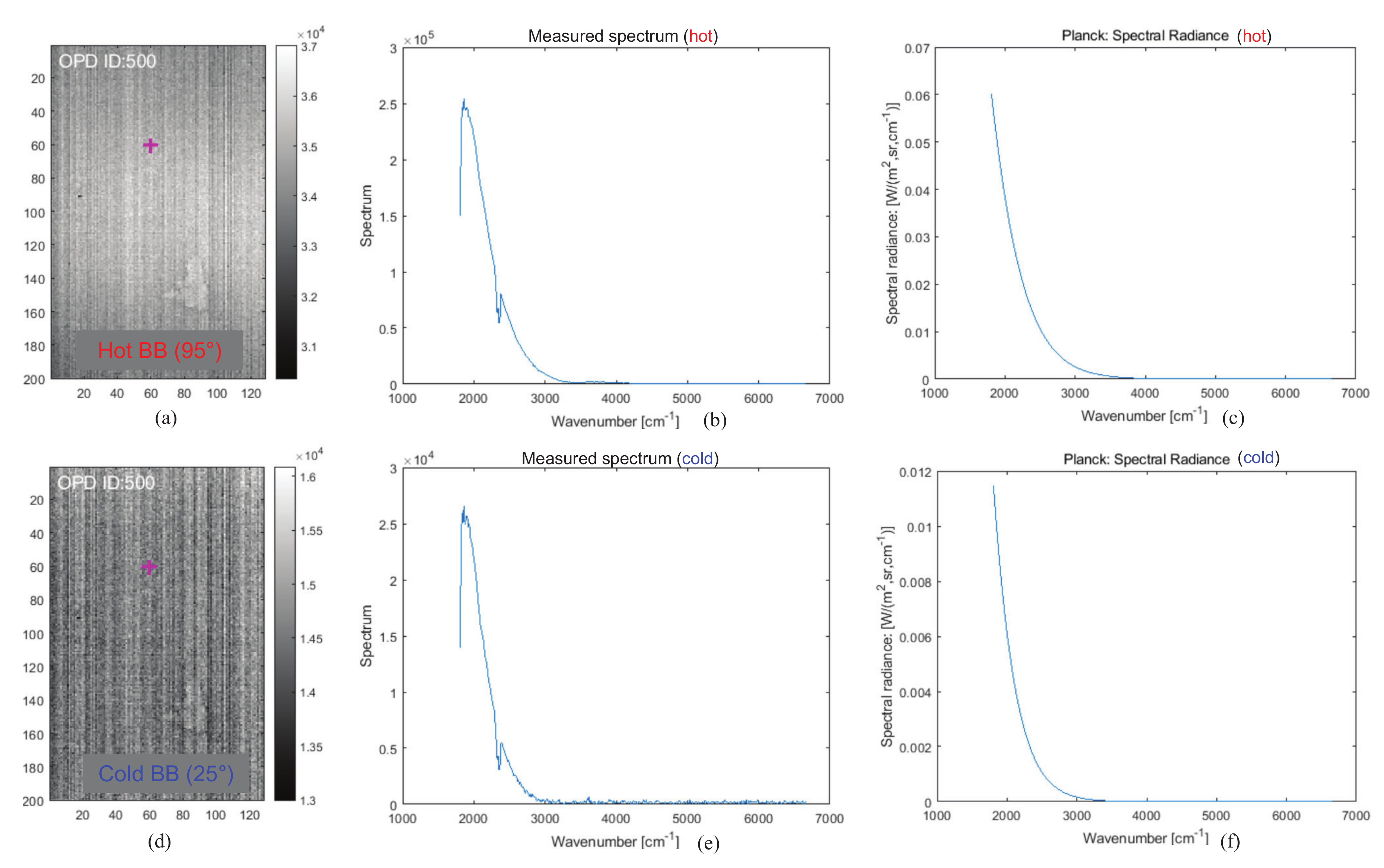
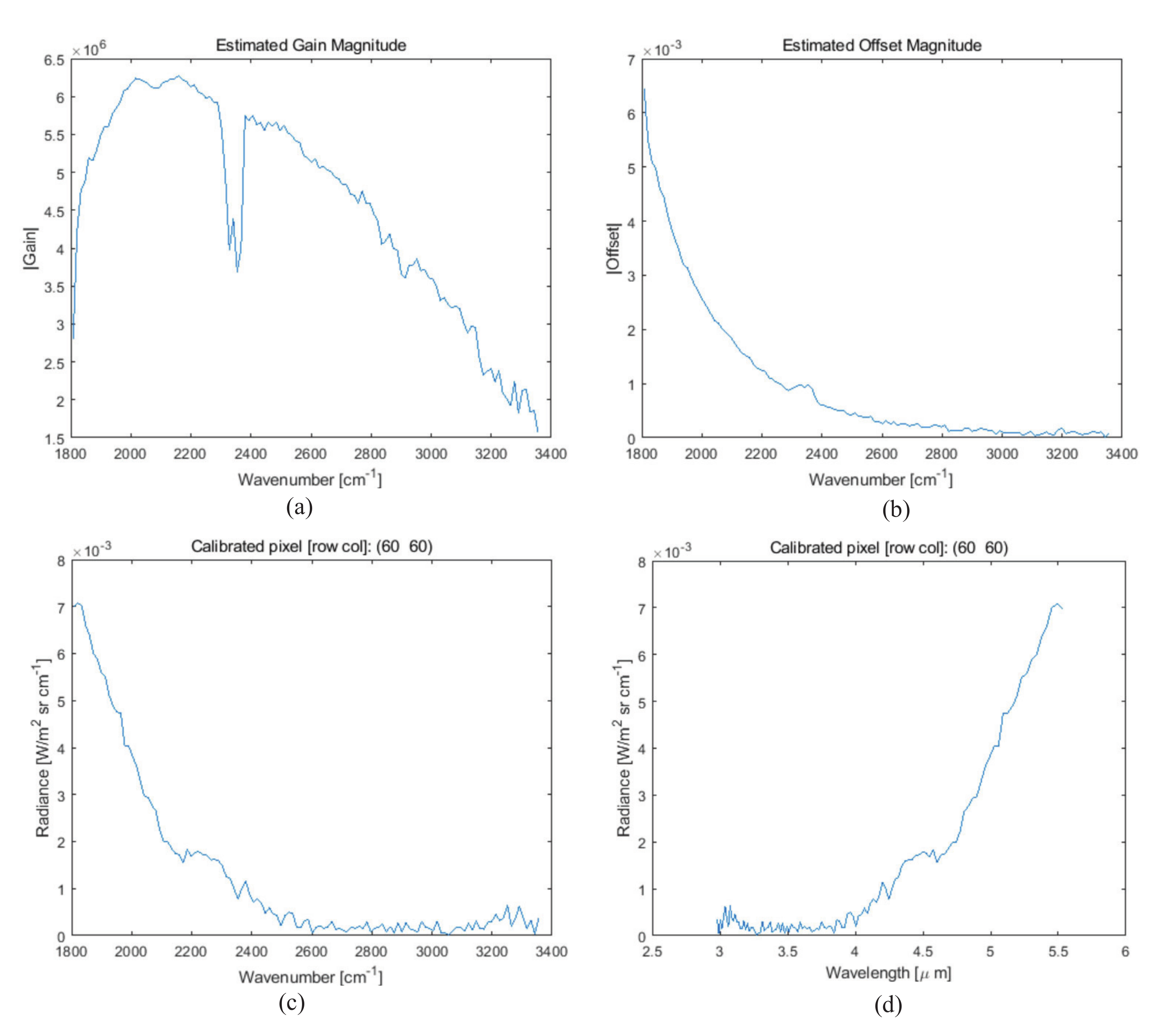
The next step is to calibrate radiometrically using two blackbodies. The HYPER-CAM MWE can provide the spectral radiance data using two built-in BBs (hot, cold) [25]. Figure 4 shows the measured interferogram image, spectra (arbitrary units), and calculated spectral radiances for the hot ($95{}^{\circ }$C) and cold ($25{}^{\circ }$C) blackbodies. Figure 5a,b show the estimated gain and offset magnitude at pixel (60, 60), respectively. Figure 5c,d presents the calculated spectral radiance with the unit of wavenumber and wavelength, respectively.

The amount of spectral radiance energy can be converted into equivalent brightness temperatures [26]. By inverting Equation (7), the temperature $T\left(K\right)$ can be obtained as

$$\begin{array}{c}\hfill T=\frac{(hc/k)\tilde{\nu }}{ln[2h{c}^2{\tilde{\nu }}^3/L_S\left(\tilde{\nu }\right)+1]}.\end{array}$$

(1)

2.4. MODTRAN Simulator

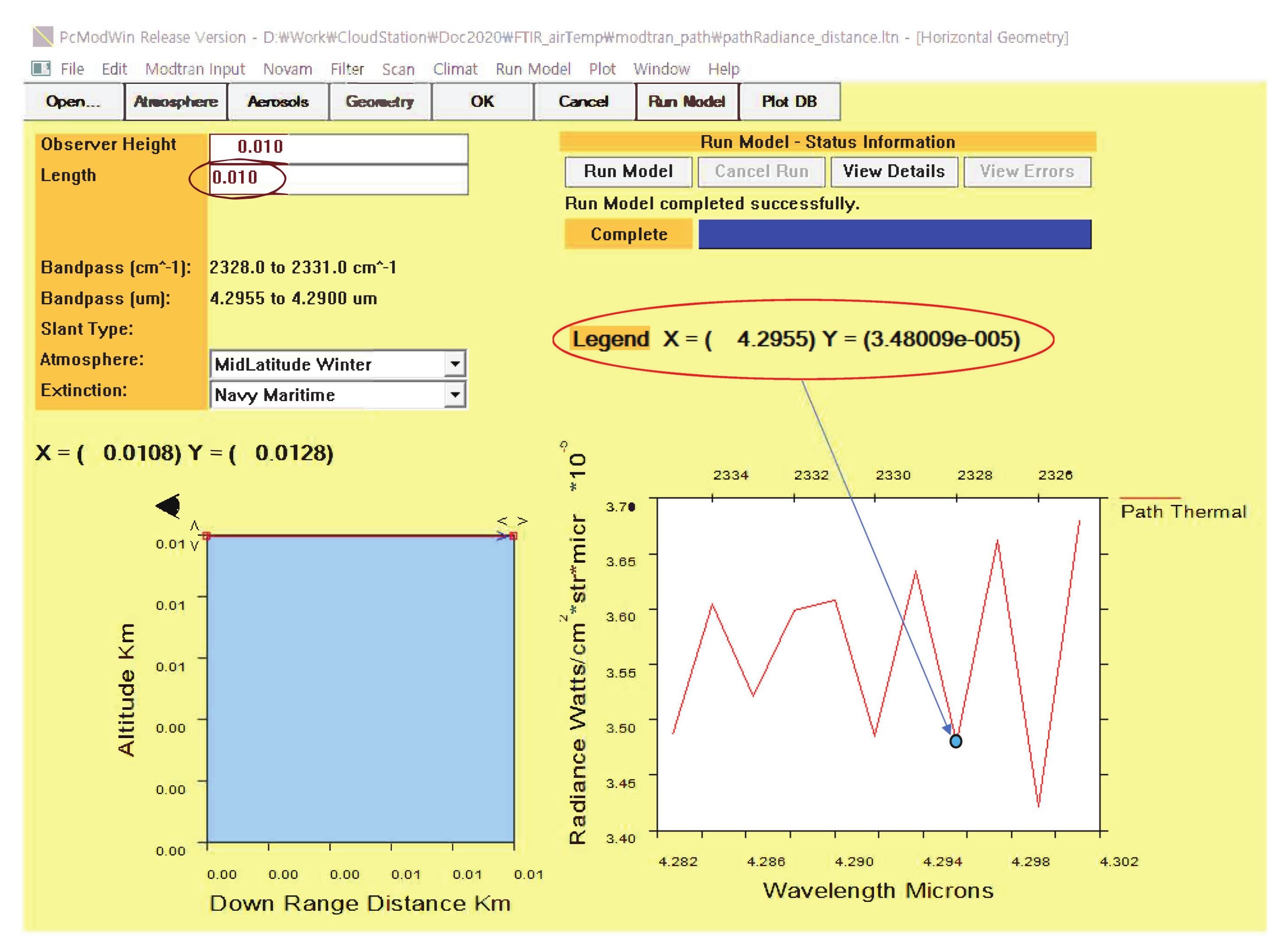
The moderate-resolution atmospheric radiance and transmittance model (MODTRAN, http://modtran.spectral.com/) is used in this paper to simulate atmospheric transmittance and path thermal calculation. Figure 6 shows a GUI interface to simulate spectral path radiance by setting geometric and atmospheric parameters.

3. Proposed Visual Air Temperature Measurement Method

3.1. Derivation of Radiative Ttransfer Equation

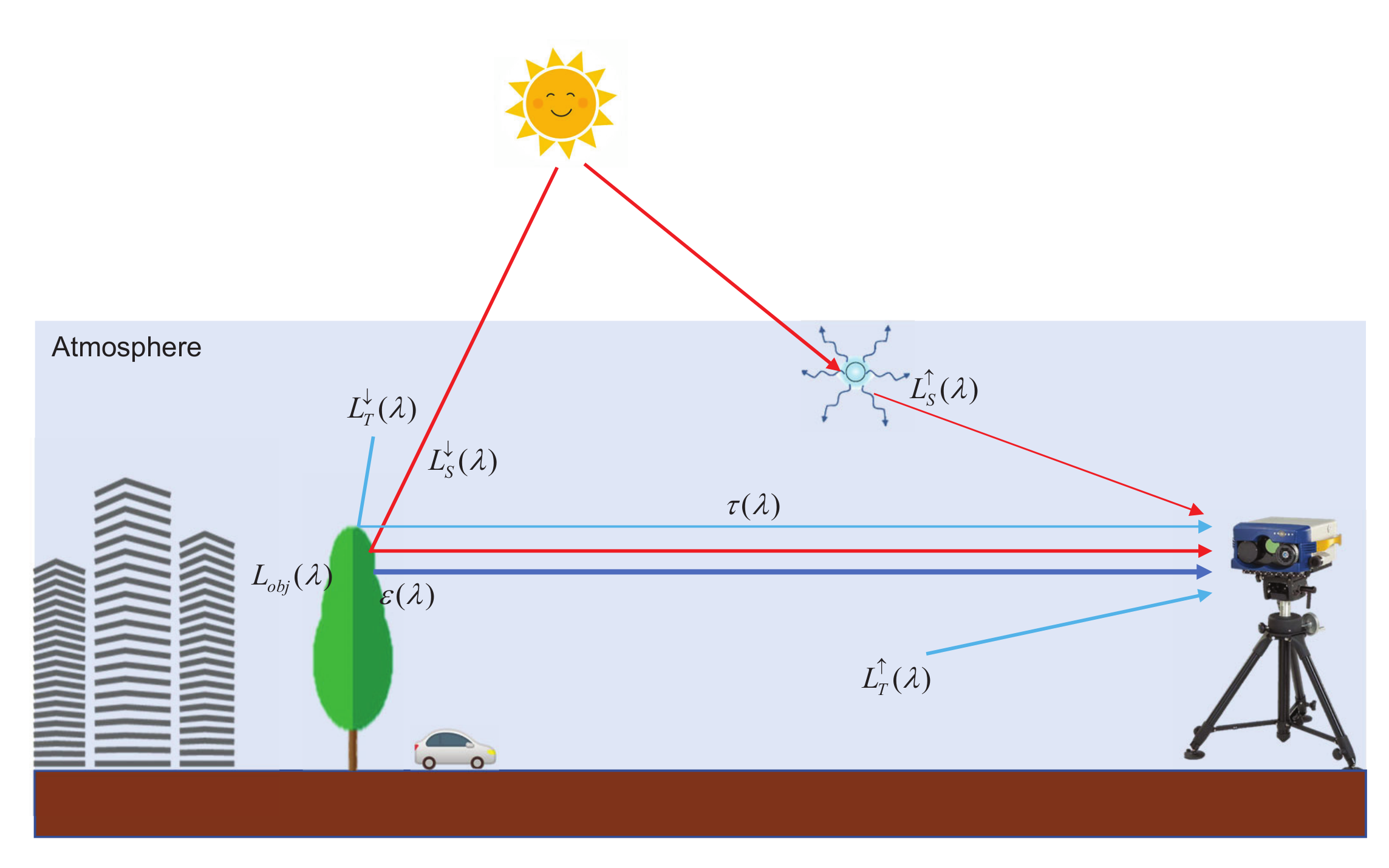
Figure 7 shows the air temperature measurement scenario. Air temperature from VisualAT measurement can be derived from radiative transfer Equation (2). We adopt the radiative transfer equation used in MODTRAN [27]. In general, at-sensor received radiance in the midwave infrared (MWIR) region consists of opaque object-emitted radiance, reflected downwelling radiance, and total atmospheric path radiance (thermal+solar components).

$$\begin{array}{c}\hfill L_{obs}\left(\lambda \right)=\tau \left(\lambda \right)\left[\epsilon \left(\lambda \right)L_{obj}(\lambda ,T_{obj})+(1-\epsilon \left(\lambda \right))(L_s^{\downarrow }\left(\lambda \right)+L_t^{\downarrow }\left(\lambda \right))\right]+L_s^{\uparrow }\left(\lambda \right)+L_t^{\uparrow }\left(\lambda \right)\end{array}$$

(2)

$L_{obs}\left(\lambda \right)$ is the at-sensor radiance; $\lambda$ is wavelenth; $\epsilon \left(\lambda \right)$ is spectral object surface emissivity; $L_{obj}(\lambda ,T_{obj})$ is the spectral radiance of the object, assuming a blackbody in the Planck function with object surface temperature ($T_{obj}$). $L_s^{\downarrow }\left(\lambda \right)$ and $L_t^{\downarrow }\left(\lambda \right)$ represent spectral downwelling solar radiance and thermal irradiance, respectively; $\tau \left(\lambda \right)$ is the spectral atmospheric transmittance, and $L_s^{\uparrow }\left(\lambda \right)$ and $L_t^{\uparrow }\left(\lambda \right)$ are the spectral upwelling solar and thermal path radiance, respectively, reaching the sensor.

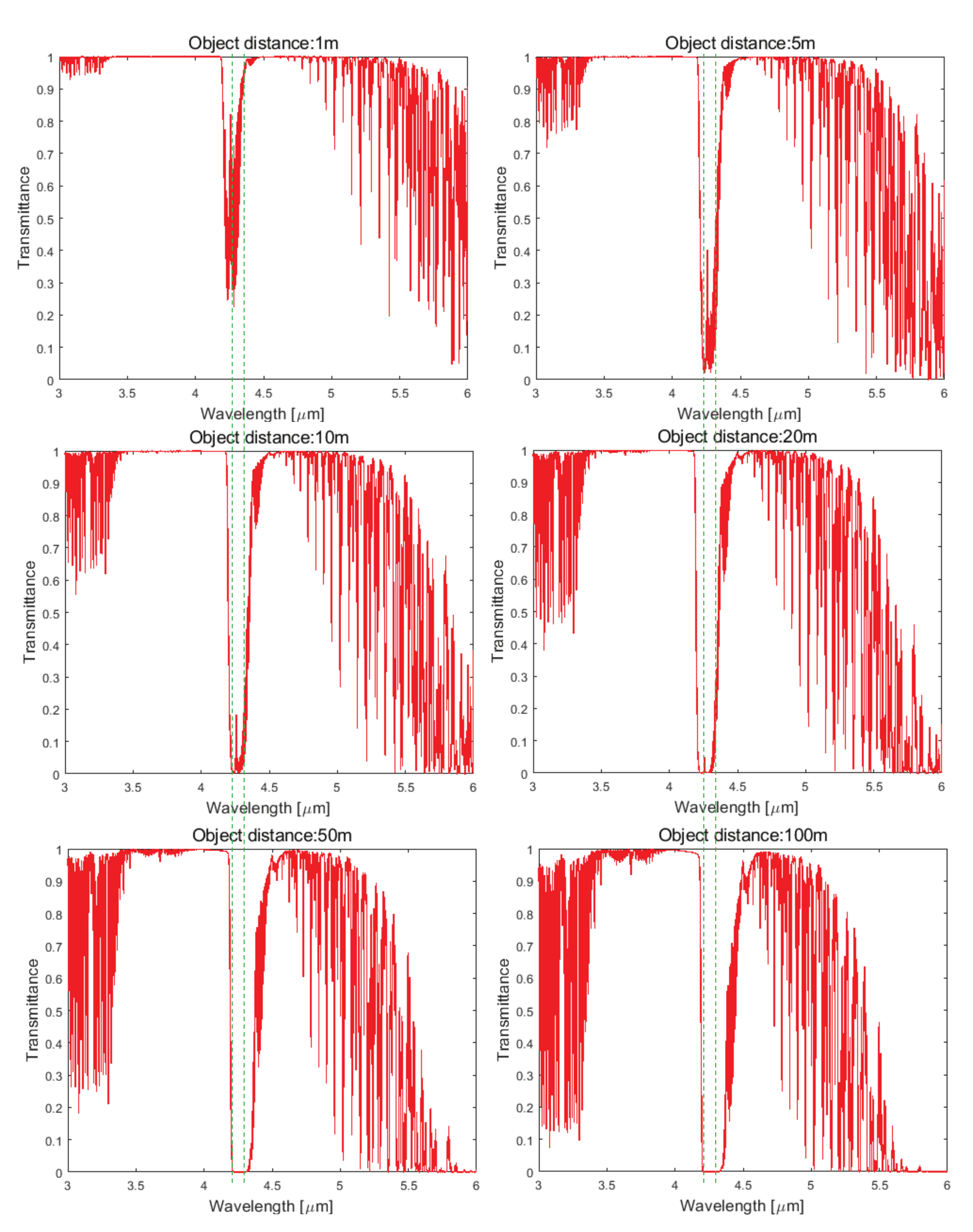
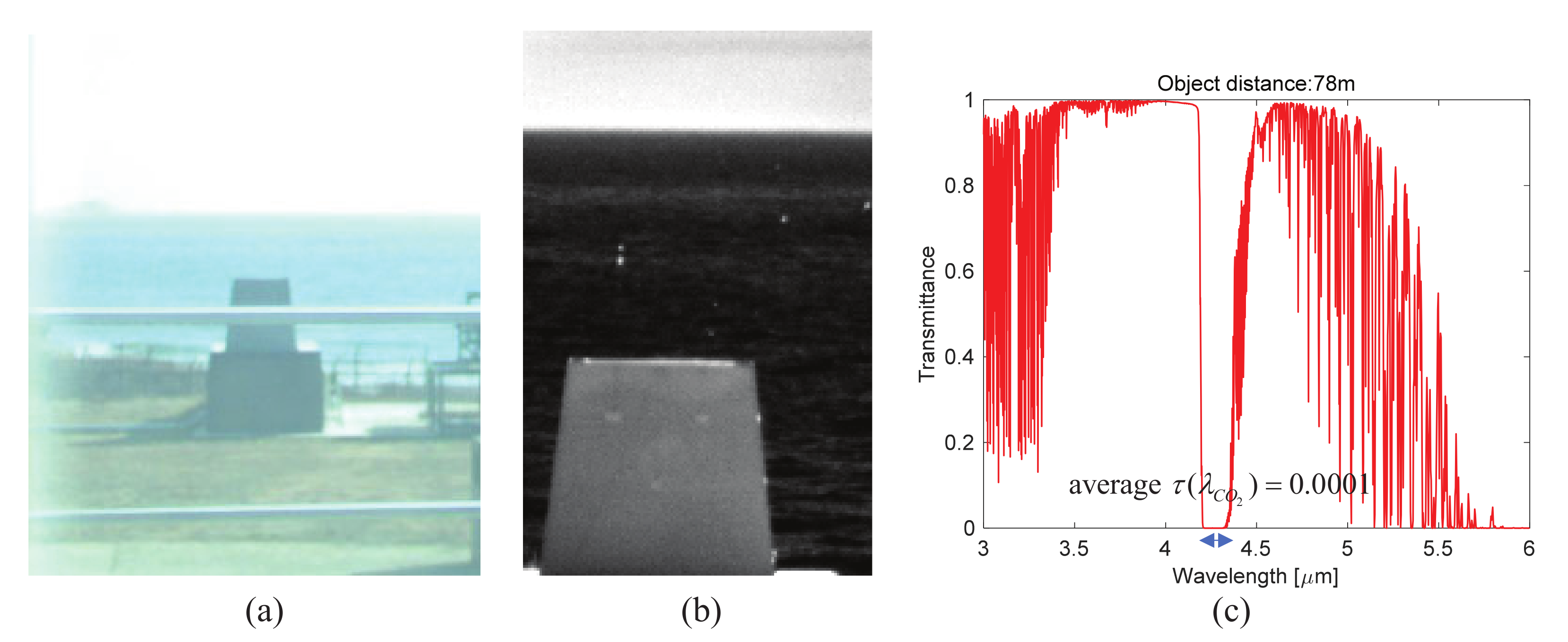
According to the MODTRAN simulation in the MWIR band, the spectral transmittance of the carbon dioxide (CO${}_2$) band (4.25–4.35 $\mathsf{\mu }$m) decreases abruptly with distance, as shown in Figure 8. The average transmittance in the CO${}_2$ band is 0.5, 0.13, 0.03, 0.005, 0.0001, and 0 at 1 m, 5 m, 10 m, 20 m, 50 m, and 100 m, respectively. If we consider only the CO${}_2$ band (${\lambda }_{C{O}_2}$) with a minimum 20 m object distance, the transmittance ($\tau \left({\lambda }_{C{O}_2}\right)$) can be regarded as 0, which leads to Equation (3). An MWIR FTIR camera receives only the upwelling of path solar and thermal radiances in the ${\lambda }_{C{O}_2}$ band where the range is normally 4.25–4.35 $\mathsf{\mu }$m.

$$\begin{array}{c}\hfill L_{obs}\left({\lambda }_{C{O}_2}\right)=L_s^{\uparrow }\left({\lambda }_{C{O}_2}\right)+L_t^{\uparrow }\left({\lambda }_{C{O}_2}\right)\end{array}$$

(3)

According to the MWIR radiometric characteristics [28], the contribution of solar radiance ($L_s^{\uparrow }({\lambda }_{C{O}_2}$)) from air scattering is very small, even for very dry conditions (less than 2% at 5 $\mathsf{\mu }$m) [28]. Ignoring the first term, we can simplify Equation (3) into Equation(4):

$$\begin{array}{c}\hfill L_{obs}\left({\lambda }_{C{O}_2}\right)=L_t^{\uparrow }\left({\lambda }_{C{O}_2}\right)\end{array}$$

(4)

The definition of thermal upwelling is defined with Equation (5):

$$\begin{array}{c}\hfill L_t^{\uparrow }\left({\lambda }_{C{O}_2}\right)=(1-\tau \left({\lambda }_{C{O}_2}\right))B({\lambda }_{C{O}_2},T_{air})\end{array}$$

(5)

Since the spectral transmittance in the CO${}_2$ band is 0 ($\tau \left({\lambda }_{C{O}_2}\right)=0$), the final form is approximated in Equation (6):

$$\begin{array}{c}\hfill L_{obs}\left({\lambda }_{C{O}_2}\right)\simeq B({\lambda }_{C{O}_2},T_{air})\end{array}$$

(6)

where $B({\lambda }_{C{O}_2},T_{air})$ denotes the spectral radiance ([W/(m${}^2·$sr$·\mathsf{\mu }$m)]) of a blackbody (Planck’s law [29]), and $T_{air}$ is the air temperature in degrees Kelvin [K] of the atmosphere between the object and the camera sensor. The spectral radiation of atmosphere is modeled as blackbody [30,31,32]. Atmospheric path radiance can be described in difference methods, but the simplest way is to model the particles as blackbodies [32]. $B({\lambda }_{C{O}_2},T_{air})$ is defined with Equation (7):

$$\begin{array}{c}\hfill B({\lambda }_{C{O}_2},T_{air})=\frac{2h{c}^2}{{\lambda }^5(e^{hc/{\lambda }_{C{O}_2}k{T}_{air}}-1)}\end{array}$$

(7)

where h denotes Planck’s constant, c is the speed of light, and k is the Boltzmann constant.

The amount of spectral radiance energy can be converted into equivalent brightness temperatures ([33]). By inverting Equation (7), temperature $T_{air}\left[K\right]$ can be obtained as follows:

$$\begin{array}{c}\hfill T_{air}\left({\lambda }_{C{O}_2}\right)=\frac{hc}{{\lambda }_{C{O}_2}kln\left(2h{c}^2/{\lambda }_{C{O}_2}^{5}B({\lambda }_{C{O}_2},T_{air})+1\right)}.\end{array}$$

(8)

3.2. VisualAT: Proposed Visual Air Temperature Measurement

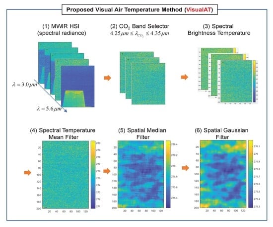
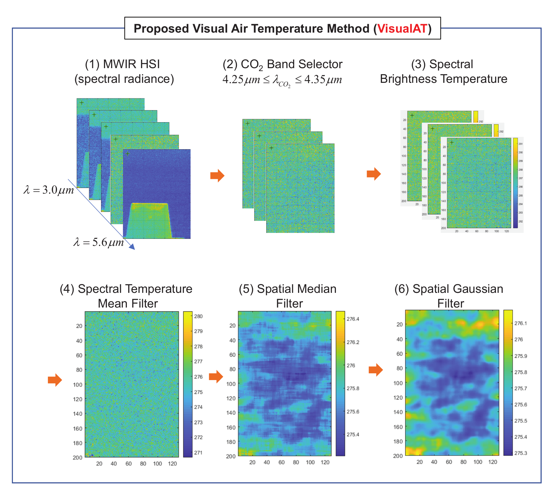
Figure 9 summarizes the overall processing flow of the proposed VisualAT method. The first row represents the three steps in spectral brightness air temperature extraction using Equation (8), described as follows.

(1)

Given is an MWIR hyperspectral image cube (374 bands, spatial resolution: $200\times 128$).

(2)

CO${}_2$ band images (4.29, 4.31, 4.34 $\mathsf{\mu }$m) are selected. The band region between 4.25–4.35 $\mathsf{\mu }$m is selected based on the MODTRAN-based transmissivity analysis ($\tau \left(\lambda \right)=0$) and visual inspection. A wavelength can be in the CO${}_2$ absorption band if there is no object signature and it looks like a noisy image.

(3)

The selected spectral radiance images are converted to spectral brightness images using Equation (8).

(3)

The second row of Figure 9 represents the image processing for visual air temperature image generation, explained in the following steps.

(4)

A raw temperature image is extracted via pixel-wise temperature mean filter along the spectral axis. It still shows a noise-like image consisting of salt-and-pepper noise and thermal noise. This can be removed by consecutive spatial 2D median filtering and Gaussian filtering [34]. The Gaussian filtering is adopted to reduce spatial thermal noise. The empirically tuned kernel size of the median filter is $10\times 15$, and sigma of the Gaussian filter is set to 2.

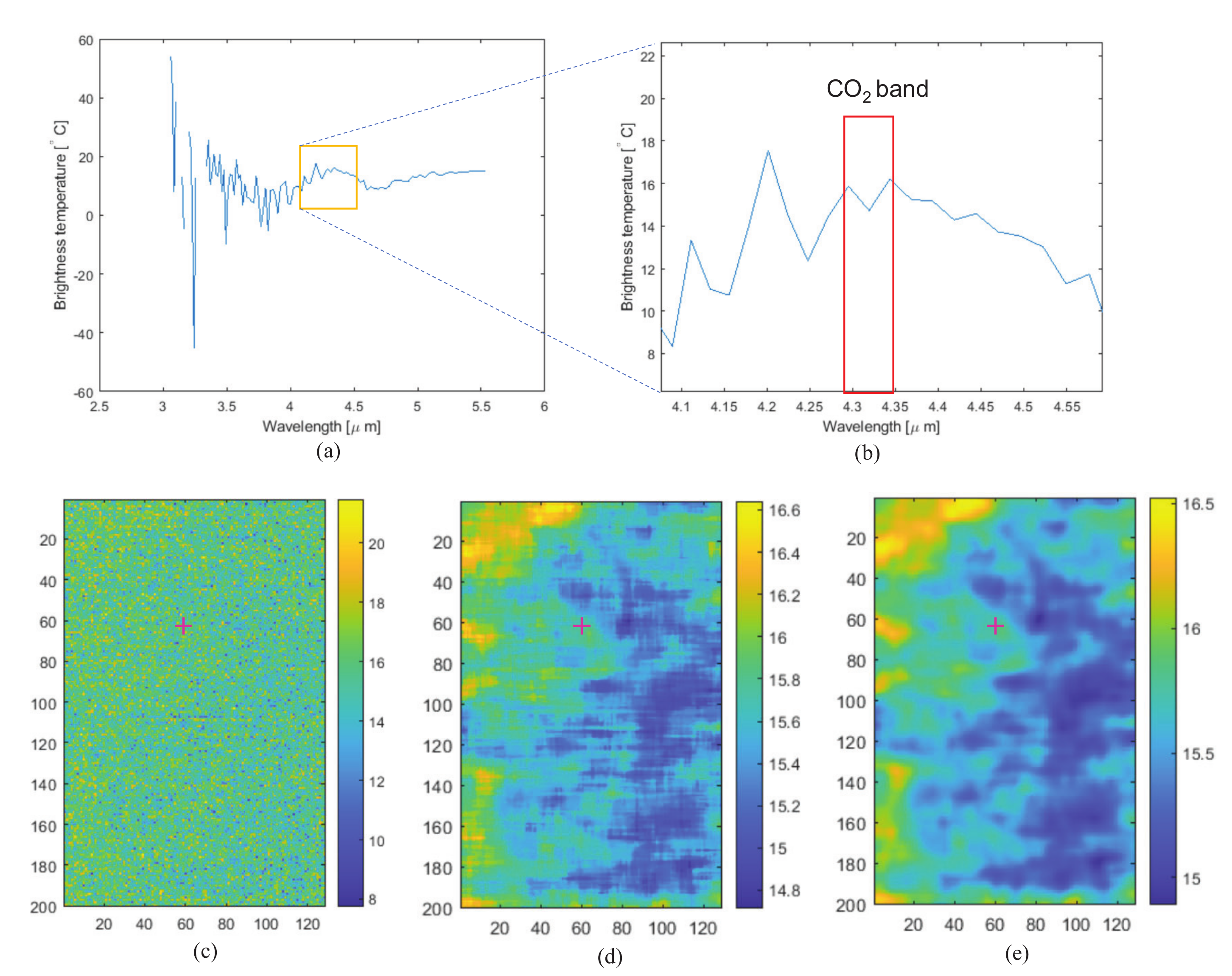
Figure 10a shows the spectral brightness temperature by applying Equation (1) to the calibrated spectral radiance at pixel (60, 60). Figure 10b shows the enlarged brightness temperature around CO${}_2$ band (4.29–4.34 $\mathsf{\mu }$m). Figure 10c represents the spatial raw temperature distribution of the CO${}_2$ band image. Final visual air temperature image (Figure 10e) is acquired through the median and Gaussian filtering processes.

3.3. Analysis of Air Temperature Measurement

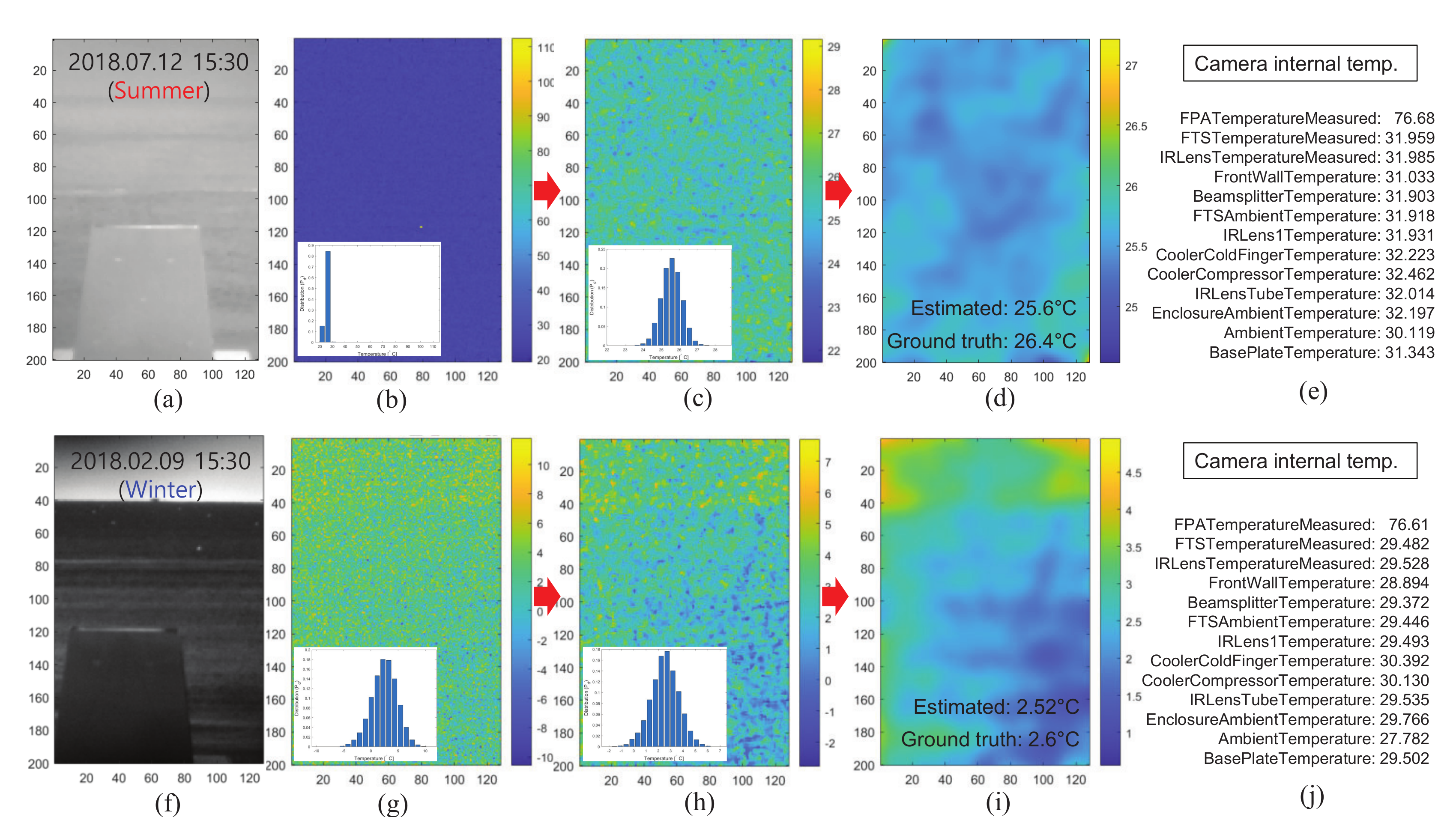
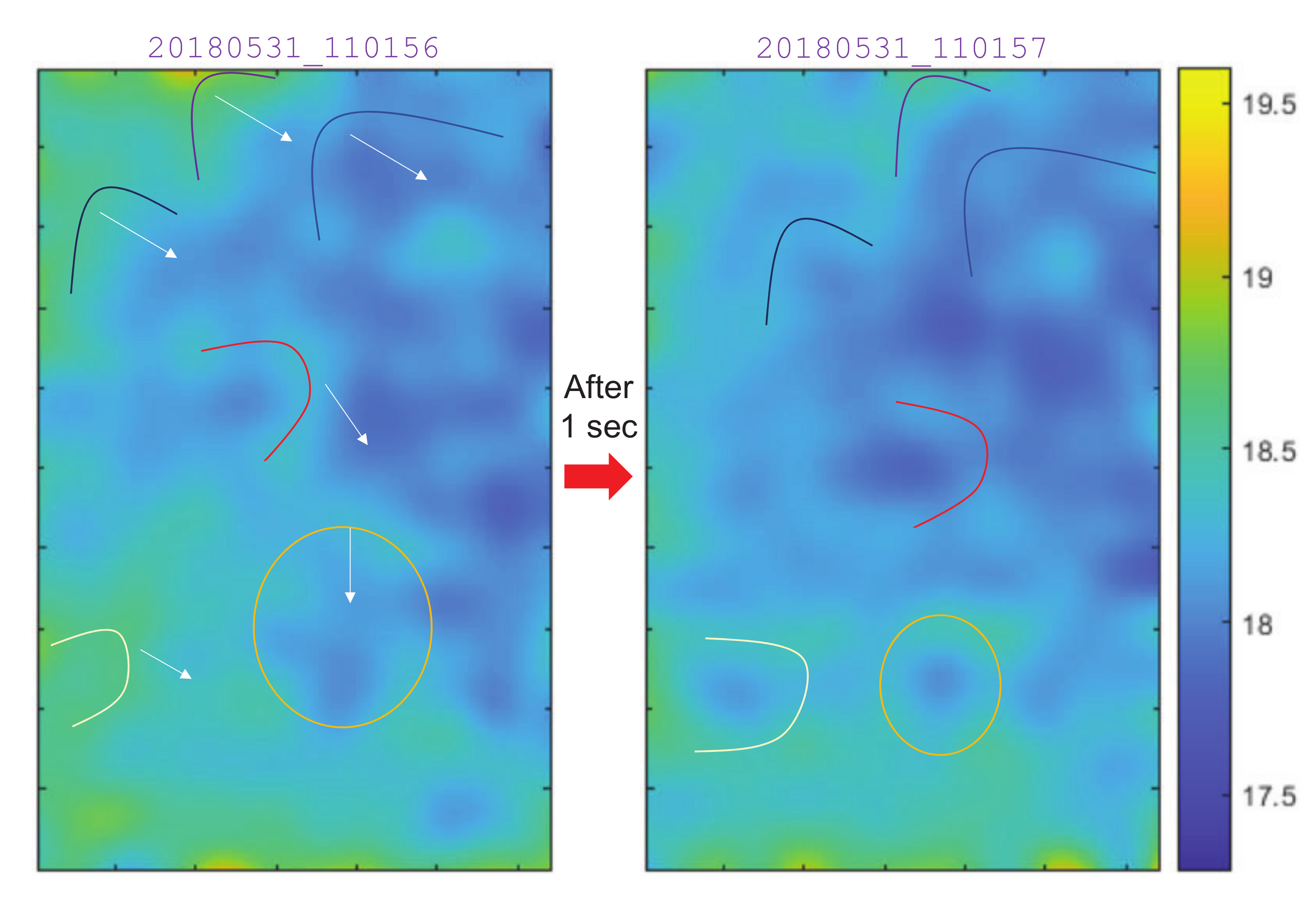
The proof of radiometric air temperature measurement and visualization is possible by mathematical derivations as Equations (2)–(8). However, it is a challenging problem to validate the air temperature measurement and visualization experimentally because we need a huge dark room with controllable air temperature. In this subsection, we analyze the properties of the VisualAT method by demonstrating extreme air temperature measurement and by thermal air flow visualization. Figure 11 demonstrates the air temperature measurement and visualization using the hot summer and cold winter data set. Upper row images represent visual temperature extraction process and camera’s internal temperature information for hot summer data. The ground truth of air temperature is $26.4{}^{\circ }$C and the estimated temperature is $25.6{}^{\circ }$C. Likewise, lower row images represent the same process for cold winter data. Note that the ground truth of air temperature is $2.6{}^{\circ }$C and the estimated temperature is $2.5{}^{\circ }$C. The internal camera temperatures of IR lens, front wall, beam splitter, and etc are approximately $29{}^{\circ }$C and they do not affect to the air temperature estimation because hot/cold blackbody-based radiometric calibration can remove the effect of stray light before each measurement. The proposed VisualAT can visualize thermal air flow using consecutive FTIR hyper-cubes acquired in very short period (1 s). Figure 12 shows the air flow directions indicated by the curves and arrows. Because the sea wind is so strong, the thermal air flow changes dynamically in very short time. Therefore, this result can be another indirect proof of imaging variations in air temperature.

3.4. Signal Analysis of Air Temperature Monitoring

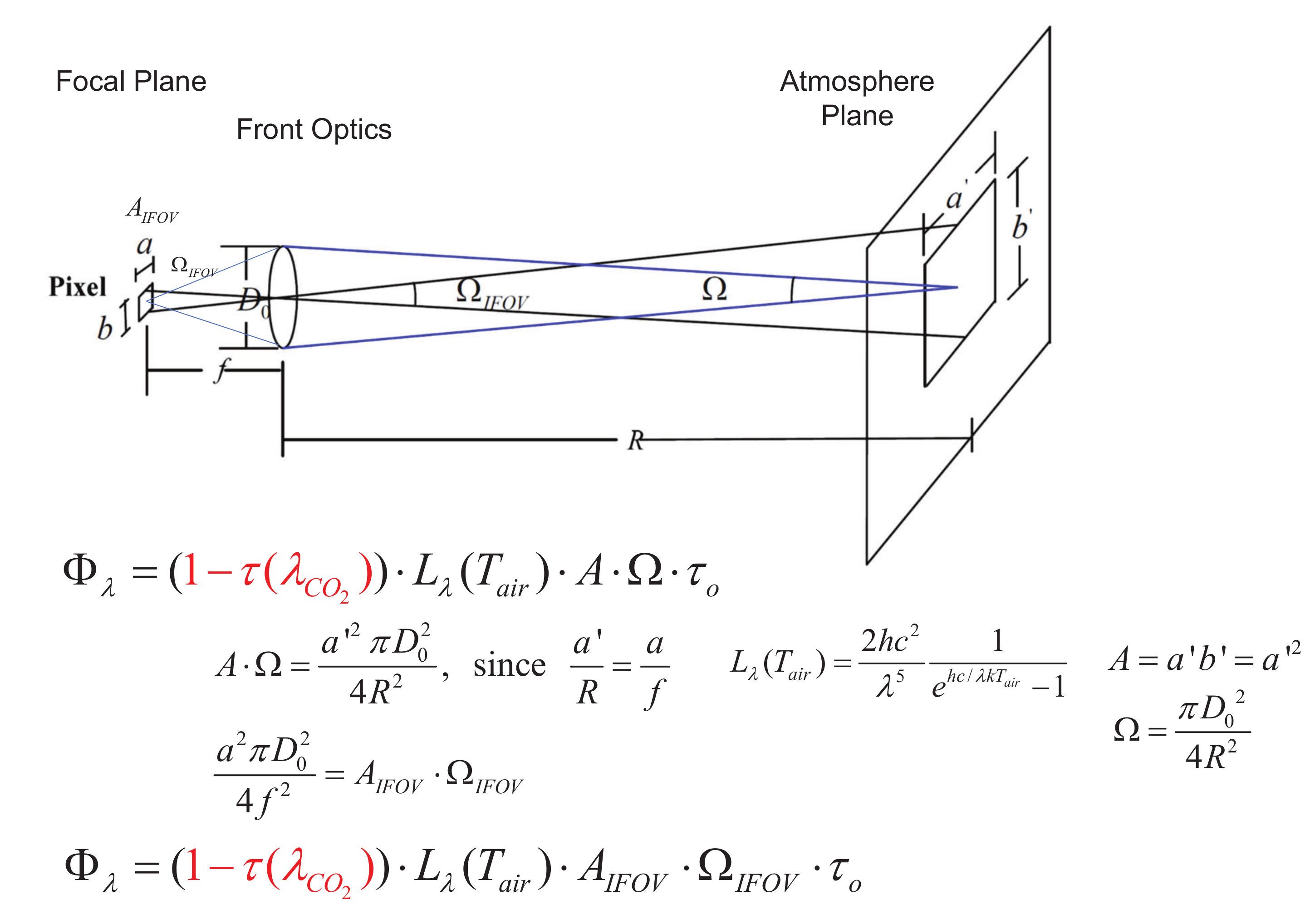
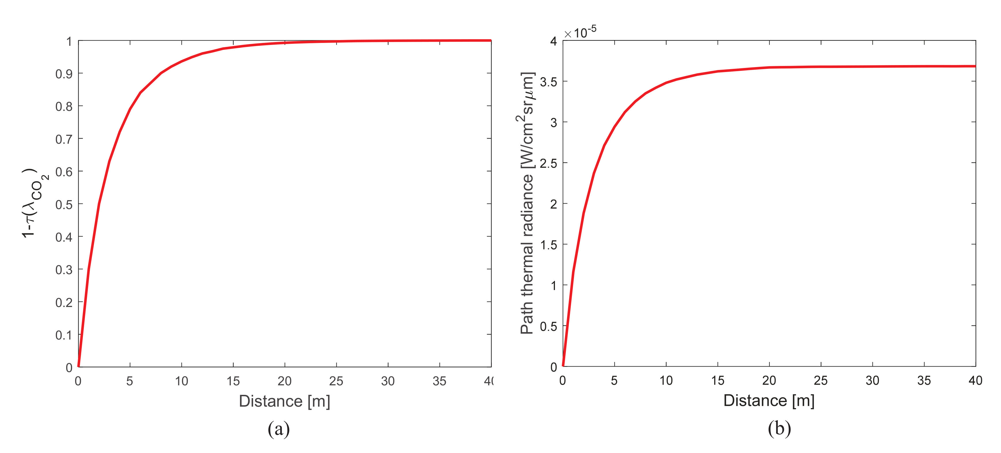
It is important to analyze how the IR radiation from different parts of the probed air contributes to the received thermal signal. Figure 13 represents the geometric relationship between atmosphere plane and a pixel. If an atmospheric plane at distance R is considered, the probing area (A) is $a^{\prime }\times b^{\prime }$ using the instantaneous field of view (IFOV). The received thermal flux (${\Phi }_{\lambda }$) at the pixel detector is ${\Phi }_{\lambda }=(1-\tau \left({\lambda }_{C{O}_2}\right))·L_{\lambda }\left(T_{air}\right)·A·\Omega ·{\tau }_o$ where $\Omega$ is solid angle and ${\tau }_o$ is lens transmittance [35]. Because air particles are regarded as blackbodies [32], the emissivity is regarded as 1. If we use basic geometrical relationships, the final form is changed to ${\Phi }_{\lambda }=(1-\tau \left({\lambda }_{C{O}_2}\right))·L_{\lambda }\left(T_{air}\right)·A_{IFOV}·{\Omega }_{IFOV}·{\tau }_o$ where $A_{IFOV}$ denotes the pixel area and ${\Omega }_{IFOV}$ represents the solid angle of IFOV. The received thermal flux is strongly related to ($1-\tau \left({\lambda }_{C{O}_2}\right)$). The simulation of atmospheric transmittance is conducted by MODTRAN 4.0 and Figure 14a represents the result. As the distance increases up to 20 m, the thermal contribution of air particles increases. This analysis is confirmed through the MODTRAN-based path thermal simulation as shown in Figure 14b and Figure 6. Therefore, we can conclude that the received air flux is contributed dominantly by the air temperature at 20 m distance.

3.5. Performance Metric

The mean absolute error (MAE) metric was used to compute the performance of the VisualAT method in predicting air temperature. The MAE metric is defined in Equation (9):

$$\begin{array}{c}\hfill MAE=\frac{1}{N}\sum _{k=1}^N\left|T_{air}^k-T_{GT}^k\right|\end{array}$$

(9)

where $T_{air}^k$ denotes the $k-th$ predicted air temperature by the VisualAT method, and $T_{GT}^k$ is the corresponding air temperature measured by the AWS, as shown in Figure 15.

Figure 16 shows the experimental environment. Figure 16a is the outdoor environment acquired via visible band camera, and Figure 16b shows a recorded broad-band image from summing all the spectral band images (1.5–5.6 $\mathsf{\mu }$m). Figure 16c represents MODTRAN-based spectral transmittance at the object distance of 78 m, and where the average transmittance of the CO${}_2$ band is 0.0001.

3.6. Parameter Analysis

A midwave hyperspectral image database was prepared for various evaluations. Hypercube images from 49 days were valid during the acquisition period (February to July 2018). In the first evaluation, the effect of the CO${}_2$ band range was important in order to estimate air temperature accurately. As summarized in Figure 17, baseline bands were selected from a visual inspection using the GUI shown in Figure 2. Top row images in Figure 17 show the spectral images corresponding to specific wavelengths. The visual selection criterion was whether the spectral image looks like it has noise in the whole image area. If atmospheric transmittance is 0, the received radiance consists of thermal path (air) radiance. Therefore, the initially selected bands were 4.22, 4.27, 4.29, 4.31, and 4.34 $\mathsf{\mu }$m. The MAE of the baseline band showed 1.32 K. If a lower band decreased to 4.20 $\mathsf{\mu }$m, the MAE decreased to 1.29 K. If the lower band increased to 4.27, 4.29, and 4.31 $\mathsf{\mu }$m individually, the corresponding MAEs were 1.26, 1.25, and 1.27 K, respectively. From these experiments, the lower band limit can be set at 4.29$\mathsf{\mu }$m. On the other hand, if we increase the upper band limit to 4.36 $\mathsf{\mu }$m with the selected lower band limit at 4.29 $\mathsf{\mu }$m, the MAE increased to 1.29 K. Therefore, we can conclude that the optimal CO${}_2$ absorption bands are 4.29, 4.31, and 4.34 $\mathsf{\mu }$m. These bands were used in the following experiments.

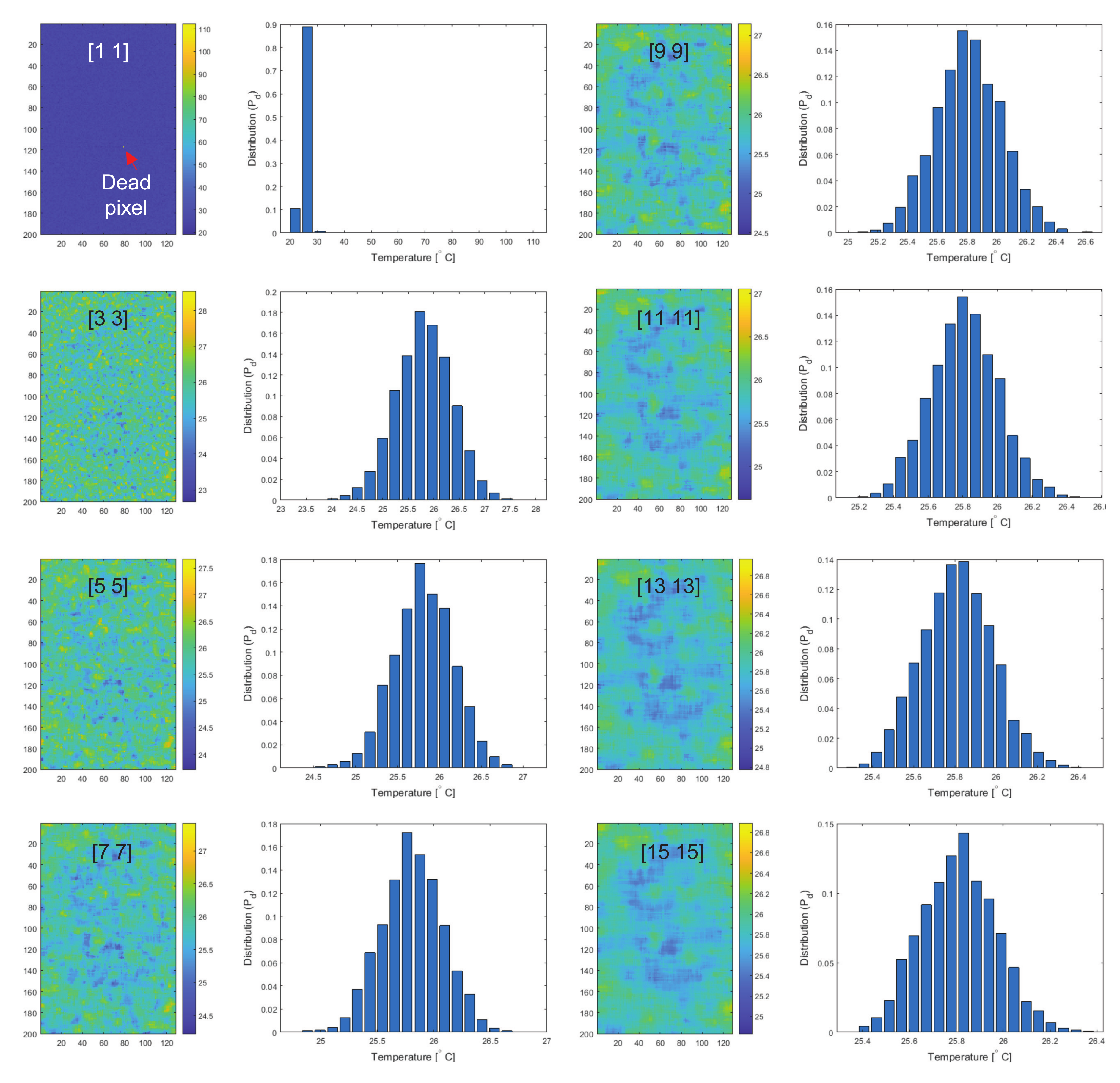
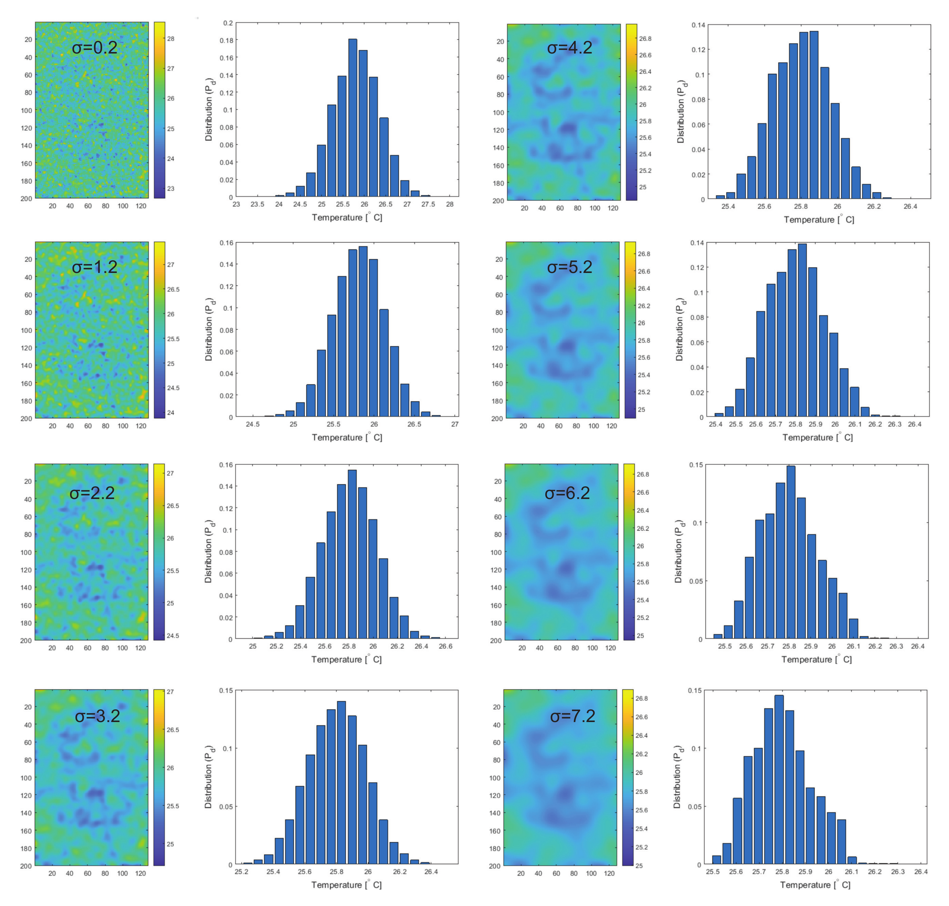
SNR can be improved additionally through the 2D median filter and 2D Gaussian filter. The 2D median filter is necessary to remove dead pixels as shown in the top-left of Figure 18 where the effects of median filter sizes from [1 1] to [15 15] were visualized. Even [3 3] median filter can remove the salt and pepper noise effectively and larger filter size can extract larger structure of air temperature distribution. The histogram distribution after the 2D median filter is Gaussian distribution, which is consensus to thermal noise distribution. True temperature signal with Gaussian noise can be estimated by Gaussian smoothing filter (unbiased, consistent linear estimator) [36]. The effects of sigma ($\sigma$) were displayed in Figure 19 where [3 3] median filter was used initially. Note that larger $\sigma$ can extract larger structure of air temperature distribution. The selection of median filter size and Gaussian filter parameter depends on application images. If salt and pepper noise is strong, larger median filter size with smaller Gaussian smoothing is suitable. If the salt and pepper noise is weak, smaller median filter size with stronger Gaussian smoothing is recommended. In this paper, we used a kernel size of $10\times 15$ for the median filter and $\sigma =2$ for the Gaussian filter because salt and pepper noise is spread horizontally and thermal noise is high.

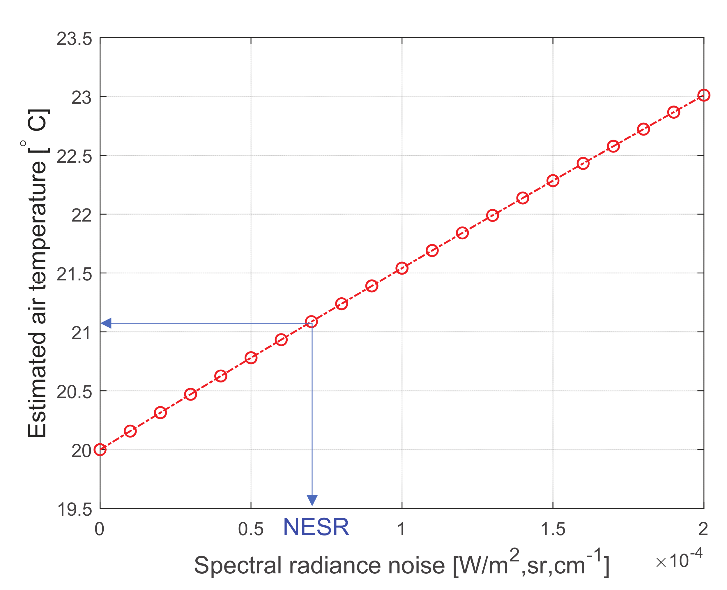
The VisualAT method depends on the spectral radiance of atmosphere. The sensitivity analysis and error propagation can be useful to understand the properties of VisualAT. The simulation is conducted by adding spectral radiance noise to Equation (7) and estimating air temperature from Equation (8). Figure 20 shows the sensitivity analysis results. The ground truth air temperature is 20 ${}^{\circ }$C and it increases linearly according to the spectral noise level. In the case of FTIR camera noise (NESR, $7\times {10}^{-5}$ [W/m${}^2$,sr,cm${}^{-1}$]), the estimated temperature is $21.08{}^{\circ }$C.

4. Experiment Results

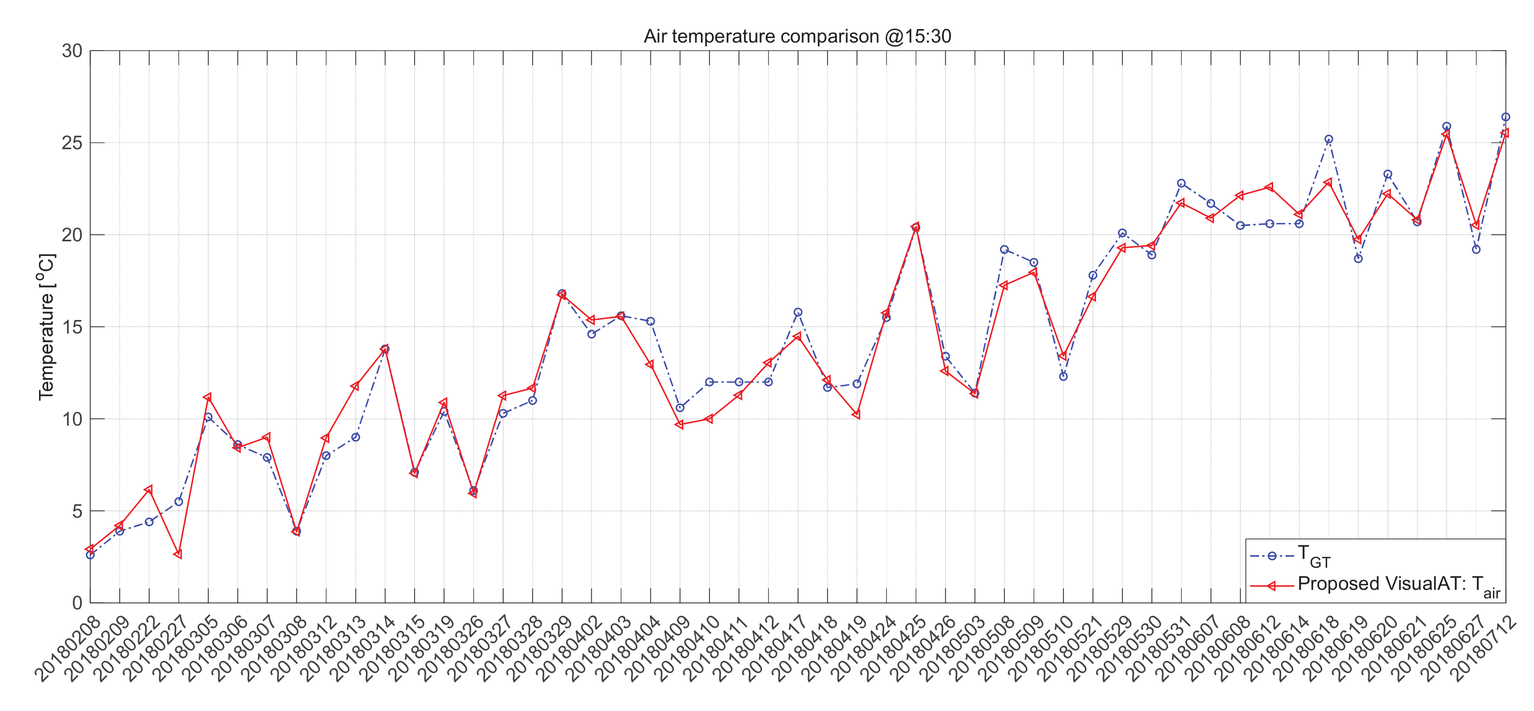
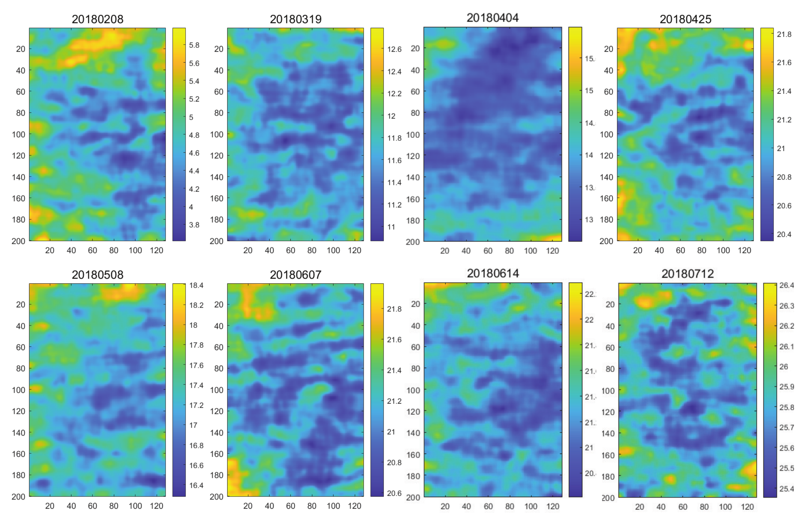
Radiometric accuracy should be evaluated to validate the usefulness of the proposed VisualAT method. Although VisualAT can present measured temperature spatially, a global mean temperature per image was extracted to compare with the ground truth air temperature recorded by the AWS. Figure 21 shows a quantitative evaluation graph between the air temperature estimated by the proposed VisualAT method and the ground truth air temperature for the 49-day dataset (acquired time: 15:30 h). The MAE was 1.25 K, which is accurate considering the remote sensing method and dynamic weather changes. The correlation coefficient between the VisualAT-based air temperature and ground truth air temperature was 0.97. Figure 22 shows representative visual air temperature images measured using the VisualAT method. To the best of our knowledge, there is no method by which to compare these results to others, and this is the first trial of instantaneous ground air temperature measurement and visualization in a ground-based approach.

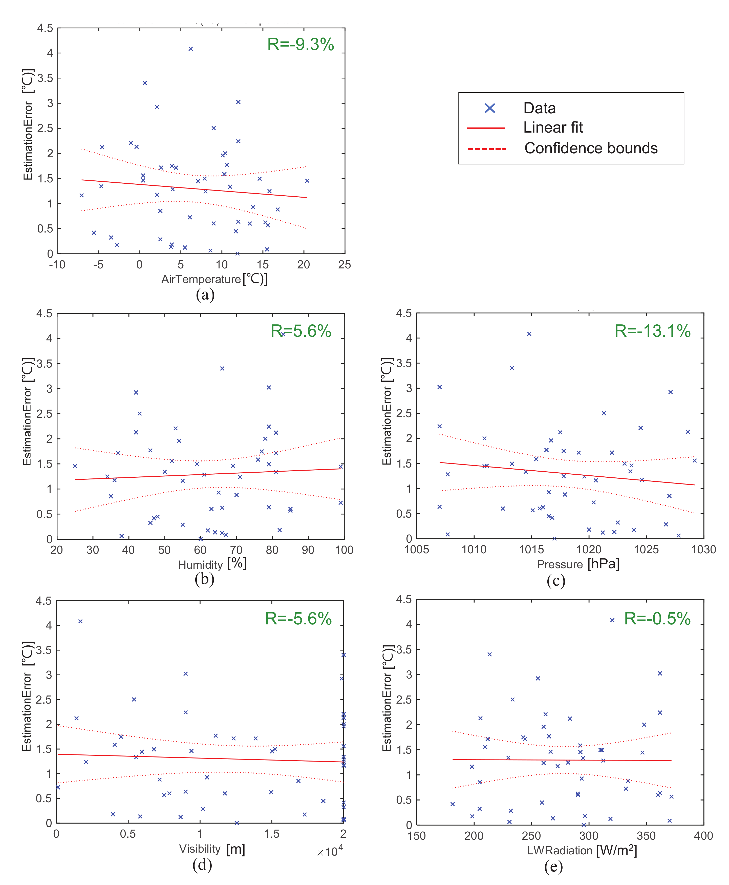
The dependency of temperature estimation accuracy from the proposed VisualAT is important in order to check robustness to various environmental changes. Figure 23 summarizes the relationships between the estimation error [${}^{\circ }$C] and other factors, such as (a) air temperature [${}^{\circ }$C], (b) humidity [%], (c) air pressure [hPa], (d) visibility [m], and (e) long-wave thermal radiation [W/m${}^2$]. The correlation coefficient (R) is annotated on the results. According to the results, the estimation error is negative relationship with air temperature, air pressure, and visibility. In addition, the error has positive relationships with humidity. This means that a more accurate temperature can be estimated if the humidity is lower. On the other hand, the long-wave thermal radiation had no specific relationship. The dependency analysis is for reference only because the data points are very scattered.

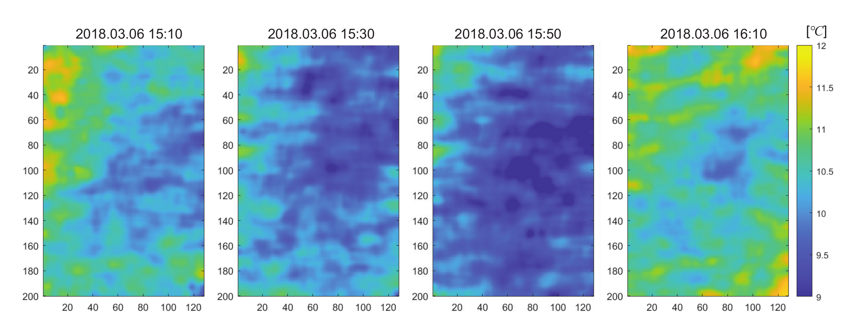
The best advantage of the proposed VisualAT method is that it can measure visual air temperature instantly. It takes approximately one second to scan a hypercube. Figure 24 shows consecutive air temperature images acquired at 20-min intervals on 6 March 2018. The color axis was set by the caxis ([7.83 9.83]) function in MATLAB for a fair temperature reading. We can see the flow of the heat flux over one hour.

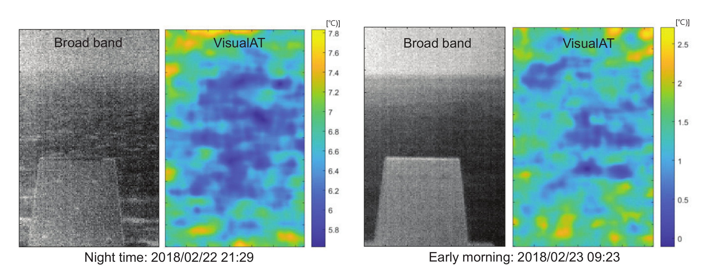
Figure 25 shows the visual air temperature images measured at night (21:29 h) and the next early morning (09:23 h). There was strong sea fog, and VisualAT can still produce air temperature images.

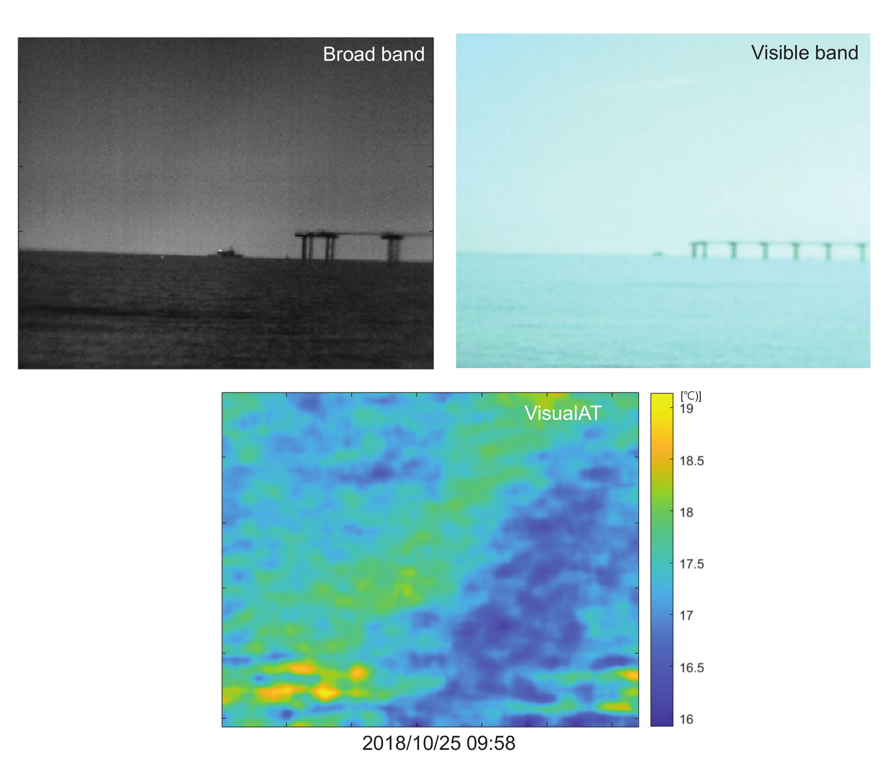
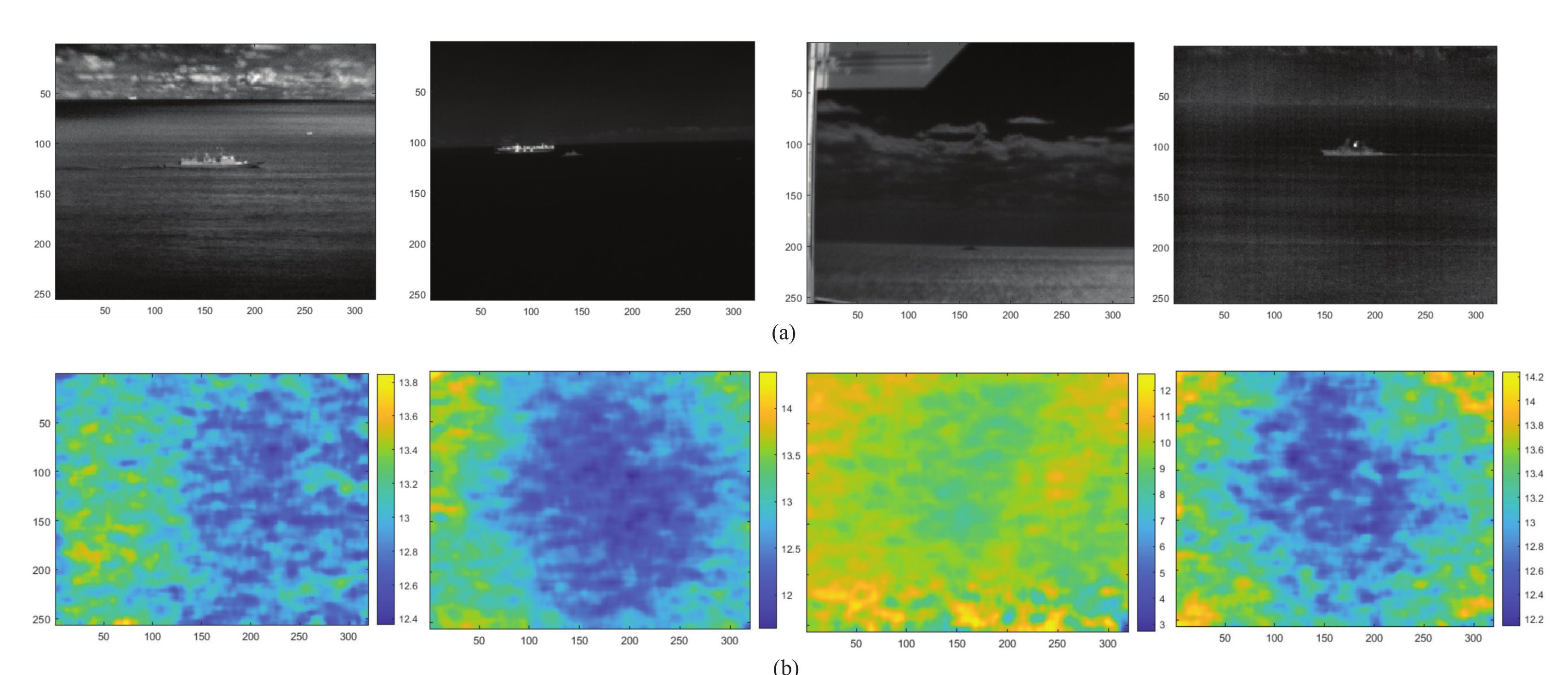
Figure 26 shows VisualAT-based remote air temperature measurement and visualization in a sea environment. Top left shows a broad-band image integrating a 1.5–5.6 $\mathsf{\mu }$m hypercube; Top right is the corresponding visible band image. The bottom image is the measured air temperature distribution from the VisualAT method. The average temperature was 16.73 ${}^{\circ }$C, and relatively hot and cold regions can be found. Figure 27 presents various air temperature visualization results in maritime environment. Different air temperature distributions can be found.

Through various analysis and evaluation, the proposed VisualAT can be a novel method to measure spatial air temperature and visualize its distribution instantly. The CO${}_2$ concentration affects to the atmospheric transmittance [37], which is related with measurement air volume. It can be a useful approach if CO${}_2$ band image is available but there are limitations such as expensive sensor system and relatively small measurement air volume (20 m distance times FOV). If there is an object in the measurement volume, the accuracy of air temperature measurement can be degraded. Partial artifact can appear when the assumption of zero atmospheric transmittance is broken. If radiometric calibration is not perfect, then internal camera device temperature can distort air temperature distribution.

5. Discussions and Conclusions

It is very challenging to measure air temperature contactlessly and instantly. This paper proposed a novel air temperature measurement and visualization method called VisualAT, which uses a midwave FTIR in the carbon dioxide absorption band. We found that spatial air temperature can be measured radiometrically by deriving the radiative transfer equation (RTE). The first physical atmospheric property is that atmospheric transmittance in the CO${}_2$ band (4.25–4.35 $\mathsf{\mu }$m) is 0.005 (at 20 m away), which can remove the effect of object and downwelling radiation. The second physical atmospheric property is that the portion of solar upwelling is very small in the CO${}_2$ band. These two properties lead to a simpler received radiance at the sensor; it is just blackbody radiance of the air temperature. The rest of the image processing, such as spectral temperature averaging, spatial median filtering, and Gaussian smoothing, produce the final visual temperature image. The proposed VisualAT method is the first to measure and visualize air temperature remotely and instantly. There is no contact sensor, no measurement delay, and no learning for regression. Based on a long-term outdoor experimentss (from February to July 2018, a valid 49 days), the proposed VisualAT method showed an MAE of 1.25 K for temperature range of 2.6–26.4 ${}^{\circ }$C. It is relatively accurate, considering all weather conditions. The measurement error has positive correlations with humidity (R = 5.6%). On the other hand, it has a negative correlation with air temperature (−9.3%), air pressure (R = −13.1%) and visibility (R = −5.6%). There is no relationship with long wave radiance (R = −0.5%). The long-range outdoor test validated the feasibility of visual air temperature measurement and visualization. According to various experiments, the VisualAT can measure air temperature correctly if there is no hot object within 20 m and proper CO${}_2$ absorption band is used. Furthermore, the precise radiometric calibration should be activated before each air temperature measurement to remove stray lights. If these conditions are satisfied, the proposed VisualAT method can be applied to spatial air temperature monitoring applications in fields such as human health, virus propagation, plant growth, climate change, hydrology, etc. In the future, we will use the air temperature information in detecting remote thermal objects.

References

- Li, L.; Li, Z.L.P. The effects of air temperature on office workers’ well-being, workload and productivity-evaluated with subjective ratings. Appl. Ergon. 2010, 42, 29–36. [Google Scholar]
- Lowen, A.C.; Steel, S.M.J.; Palese, P. Influenza virus transmission is dependent on relative humidity and temperature. PLoS Pathog. 2007, 3, 1–7. [Google Scholar] [CrossRef] [PubMed]
- Hatfield, J.L.; Prueger, J.H. Temperature extremes: Effect on plant growth and development. Weather Clim. Extrem. 2015, 10, 4–10. [Google Scholar] [CrossRef] [Green Version]
- Robeson, S.M. Relationships between mean and standard deviation of air temperature: Implications for global warming. Clim. Res. 2002, 22, 205–213. [Google Scholar] [CrossRef]
- Lin, S.; Moore, N.J.; Messina, J.P.; DeVisser, M.H.; Wu, J. Evaluation of estimating daily maximum and minimum air temperature with MODIS data in east Africa. Int. J. Appl. Earth Obs. Geoinf. 2012, 18, 128–140. [Google Scholar] [CrossRef]
- Mukherjee, R.; Basu, J.; Mandal, P.; Guha, P.K. A review of micromachined thermal accelerometers. J. Micromech. Microeng. 2017, 27, 123002. [Google Scholar] [CrossRef] [Green Version]
- Pollock, D.D. Thermocouples: Theory and Properties; CRC Press: Boca Raton, FL, USA, 1991. [Google Scholar]
- Pivovarník, M.; Khalsa, S.J.S.; Jiménez-Muñoz, J.C.; Zemek, F. Improved Temperature and Emissivity Separation Algorithm for Multispectral and Hyperspectral Sensors. IEEE Trans. Geosci. Remote Sens. 2017, 55, 1944–1953. [Google Scholar] [CrossRef]
- Li, Z.L.; Becker, F.; Stoll, M.P.; Wan, Z. Evaluation of Six Methods for Extracting Relative Emissivity Spectra from Thermal Infrared Images. Remote Sens. Environ. 1999, 69, 197–514. [Google Scholar] [CrossRef]
- Khopkar, P.; Agnihotri, S. Modelling Temperature-Vegetation Index (TVX) space and Quality of Life (QoL) for enhanced change detection analysis: A Case Study of Ahmedabad City. In Proceedings of the 38th Asian Conference on Remote Sensing (ACRS), New Delhi, India, 23–27 October 2017. [Google Scholar]
- Parviz, L.; Kholghi, M.; Valizadeh, K.H. Estimation of Air Temperature Using Temperature-Vegetation Index (TVX) Method. J. Water Soil Sci. 2011, 15, 21–34. [Google Scholar]
- Hou, P.; Chen, Y.; Jiang, W.Q.G.C.W.; Li, J. Near-surface air temperature retrieval from satellite images and influence by wetlands in urban region. Appl. Climatol. 2013, 111, 109–118. [Google Scholar] [CrossRef]
- Sun, Y.J.; Wang, J.F.; Zhang, R.H.; Gillies, R.R.; Xue, Y.; Bo, Y.C. Air temperature retrieval from remote sensing data based on thermodynamics. Theor. Appl. Climatol. 2005, 80, 37–48. [Google Scholar] [CrossRef]
- Shi, Y.; Jiang, Z.; Dong, L.; Shen, S. Statistical estimation of high-resolution surface air temperature from MODIS over the Yangtze River Delta. China. J. Meteorol. Res. 2017, 31, 448–454. [Google Scholar] [CrossRef]
- Shen, H.; Jiang, Y.; Li, T.; Cheng, Q.; Zeng, C.; Zhang, L. Deep learning-based air temperature mapping by fusing remote sensing, station, simulation and socioeconomic data. Remote Sens. Environ. 2020, 240, 111692. [Google Scholar] [CrossRef] [Green Version]
- Liu, S.; Su, H.; Zhang, R.; Tian, J.; Wang, W. Estimating the Surface Air Temperature by Remote Sensing in Northwest China Using an Improved Advection-Energy Balance for Air Temperature Model. Adv. Meteorol. 2015, 2016, 4294219. [Google Scholar] [CrossRef] [Green Version]
- Lu, N.; Liang, S.; Huang, G.; Qin, J.; Yao, L.; Wang, D.; Yang, K. Hierarchical Bayesian space-time estimation of monthly maximum and minimum surface air temperature. Remote Sens. Environ. 2018, 211, 48–58. [Google Scholar] [CrossRef]
- Hooker, J.; Duveiller, G.; Cescatti, A. Data Descriptor: A global dataset of air temperature derived from satellite remote sensing and weather stations. Sci. Data 2018, 5, 180246. [Google Scholar] [CrossRef] [PubMed] [Green Version]
- Wang, X.; OuYang, X.; Li, Z.L.; Zhang, R. A New Method for Temperature/Emissivity Separation from Hyperspectral Thermal Infrared Data. In Proceedings of the 2008 IEEE International Geoscience and Remote Sensing Symposium IGARSS 2008), Boston, MA, USA, 8–11 July 2008; pp. III-286–III-289. [Google Scholar] [CrossRef]
- Wang, H.; Xiao, Q.; Li, H.; Zhong, B. Temperature and emissivity separation algorithm for TASI airborne thermal hyperspectral data. In Proceedings of the 2011 International Conference on Electronics, Communications and Control (ICECC), Ningbo, China, 9–11 September 2011; pp. 1075–1078. [Google Scholar] [CrossRef]
- Tan, K.; Liao, Z.; Du, P.; Wu, L. Land surface temperature retrieval from Landsat 8 data and validation with geosensor network. Front. Earth Sci. 2017, 11, 20–34. [Google Scholar] [CrossRef]
- Harig, R. Passive remote sensing of pollutant clouds by Fourier-transform infrared spectrometry: Signal-to-noise ratio as a function of spectral resolution. Appl. Opt. 2004, 43, 4603–4610. [Google Scholar] [CrossRef] [PubMed]
- Gagnon, M.A.; Gagnon, J.P.; Tremblay, P.; Savary, S.; Farley, V.; Éric, G.; Lagueux, P.; Chamberland, M. Standoff midwave infrared hyperspectral imaging of ship plumes. Proc. SPIE 2016, 9988, 998806. [Google Scholar] [CrossRef]
- Kim, S.; Kim, J.; Lee, J.; Ahn, J. Midwave FTIR-Based Remote Surface Temperature Estimation Using a Deep Convolutional Neural Network in a Dynamic Weather Environment. Micromachines 2018, 9, 495. [Google Scholar] [CrossRef] [Green Version]
- Schlerf, M.; Rock, G.; Lagueux, P.; Ronellenfitsch, F.; Gerhards, M.; Hoffmann, L.; Udelhoven, T. A Hyperspectral Thermal Infrared Imaging Instrument for Natural Resources Applications. Remote Sens. 2012, 4, 3995–4009. [Google Scholar] [CrossRef] [Green Version]
- Trishchenko, A.P. Solar Irradiance and Effective Brightness Temperature for SWIR Channels of AVHRR/NOAA and GOES Imagers. J. Atmos. Ocean. Technol. 2006, 23, 198–210. [Google Scholar] [CrossRef]
- Romaniello, V.; Spinetti, C.; Silvestri, M.; Buongiorno, M.F. A Sensitivity Study of the 4.8 um Carbon Dioxide Absorption Band in the MWIR Spectral Range. Remote Sens. 2020, 12, 172. [Google Scholar] [CrossRef] [Green Version]
- Griffin, M.K.; Hua, K.; Burke, H.; Kerekes, J.P. Understanding radiative transfer in the midwave infrared: A precursor to full-spectrum atmospheric compensation. Proc. SPIE 2004, 5425, 348–356. [Google Scholar] [CrossRef]
- Andrews, D. An Introduction to Atmospheric Physics; Cambridge Press: Cambridge, UK, 2000. [Google Scholar]
- Hohn, D.H. Atmospheric Vision 0.35 um < x < 14 um. Appl. Opt. 1975, 14, 404–412. [Google Scholar]
- Sobrino, J.; Li, Z.L.; Stoll, P.; Becker, F. Multi-channel and multi-angle algorithms for estimating sea and land surface temperature with ATSR data. Int. J. Remote Sens. 2004, 17, 2089–2114. [Google Scholar] [CrossRef]
- Driggers, R.G.; Friedman, M.H.; Nichols, J. Introduction to Infrared and Electro-Optical Systems; ARTECH HOUSE: Washington, DC, USA, 2012. [Google Scholar]
- Eismann, M.T. Hyperspectral Remote Sensing; SPIE Press: Bellingham, WA, USA, 2012. [Google Scholar]
- Gonzalez, R.C.; Woods, R.E. Digital Image Processing, 4th ed.; Pearson: London, UK, 2012. [Google Scholar]
- Iersel, M.V.; Mack, A.; Degache, M.A.C.; Eijk, A.M.J.V. Ship plume modelling in EOSTAR. Proc. SPIE 2014, 9242, 92421S. [Google Scholar]
- Papoulis, A.; Pillai, U. Probability, Random Variables and Stochastic Processes, 4th ed.; McGraw-Hill Europe: New York, NY, USA, 2002. [Google Scholar]
- Wei, P.S.; Hsieh, Y.C.; Chiu, H.H.; Yen, D.L.; Lee, C.; Tsai, Y.C.; Ting, T.C. Absorption coefficient of carbon dioxide across atmospheric troposphere layer. Heliyon 2018, 4, 1–20. [Google Scholar] [CrossRef] [Green Version]
Figure 1.
Measurement scenario in an outdoor environment: FTIR is located in an air conditioned room and AWS is installed on the roof. The background scene is 78 m away from the camera.
Figure 2.
Midwave FTIR image analysis software platform. A spectral image at a selected wavelength can be visualized interactively.
Figure 3.
Spectral calibration process: (a) interferogram image at optical path difference (OPD) ID = 500 (ZPD); (b) interferogram at a pixel ((row, col) = (60, 60)); (c) fast Fourier transform (FFT) results; (d) wavenumber calibration results.
Figure 4.
Blackbody spectrum and spectral radiance extraction for a radiometric calibration: (a) interferogram image of a hot blackbody (C); (b) measured spectrum of a hot blackbody; (c) calculated spectral radiance at hot temperature; (d) interferogram image of a cold blackbody (C); (e) mesured spectrum of a cold blackbody; (f) calculated spectral radiance at cold temperature.
Figure 5.
Radiometric calibration and spectral radiance extraction: (a) estimated gain magnitude; (b) estimated offset magnitude; (c) spectral radiance vs. wavenumber; (d) spectral radiance vs. wavelength.
Figure 6.
MODTRAN simulation environment for path thermal calculation.
Figure 7.
Operational concept of visual air temperature (VisualAT) measurement using the passive open path Fourier transform infrared (FTIR) imaging system.
Figure 8.
Spectral transmittance according to object-camera distance in the MWIR band. Note the abrupt absorption at 4.25–4.35 m.
Figure 9.
Overall processing flow of visual air temperature (VisualAT) measurement method.
Figure 10.
Brightness temperature extraction and VisualAT results: (a) brightness temperature; (b) enlarged brightness temperature with CO band region; (c) CO band image; (d) median filtered image; (e) Gaussian filtered temperature image.
Figure 11.
Indirect proof of air temperature measurement by extreme weather conditions: Hot summer-(a) broad-band image, (b) CO band image, (c) median filtered image, (d) Gaussian filtered image, (e) camera internal temperature information; Cold winder-(f) broad-band image, (g) CO band image, (h) median filtered image, (i) Gaussian filtered image, (j) camera internal temperature information.
Figure 12.
Indirect proof of air temperature measurement by air flow visualization. The arrows indicate the directions of air flow.
Figure 13.
Geometrical model of received thermal flux in a pixel.
Figure 14.
(a) (1-atmospheric transmittance) vs. distance (MODTRAN-based simulation at CO absorption band (4.29 m)), (b) path thermal radiance vs. distance (MODTRAN-based simulation).
Figure 15.
AWS information: date and time; wind speed, maximum wind speed, average wind direction, and maximum wind direction; air temperature, humidity, and pressure; and visibility.
Figure 16.
An example of experiment environment: (a) outdoor environment acquired by a visible band camera, (b) broad-band infrared image, and (c) spectral transmittance in MWIR band.
Figure 17.
CO band range selection results: Baseline band is selected by visual inspection and the optimal band range is selected by maximizing mean absolute error (MAE) metric.
Figure 18.
Spatial effects of 2D median filter size and histogram distribution.
Figure 19.
Spatial effects of 2D Gaussian filter with .
Figure 20.
Spectral noise and estimated air temperature analysis.
Figure 21.
Quantitative evaluation graph of the proposed VisualAT method for the whole database acquired from February to July 2018.
Figure 22.
Examples of air temperature images measured by the proposed VisualAT method for different months (from February 2018–July2018).
Figure 23.
Examples of air temperature images measured by the proposed VisualAT method for different months: (a) estimation error vs. air temperature; (b) estimation error vs. humidity; (c) estimation error vs. pressure; (d) estimation error vs. visibility; (e) estimation error vs. long wave thermal radiation.
Figure 24.
VisualAT-based dynamic temperature images measured at different times (20-min. intervals): Temporal variation of air temperature distribution can be found.
Figure 25.
Example of visual air temperature images at night and in the morning: (left) night time air temperature image at 21:29; (right) early morning temperature image at 09:23.
Figure 26.
Remote air temperature image visualization example from an outdoor sea environment: (top left) broad band image; (top right) visible band image, (bottom) VisualAT-based air temperature image.
Figure 27.
Various remote air temperature image visualization example in maritime environment: (a) broadband images; (b) corresponding VisualAT images.
© 2020 by the author. Licensee MDPI, Basel, Switzerland. This article is an open access article distributed under the terms and conditions of the Creative Commons Attribution (CC BY) license (http://creativecommons.org/licenses/by/4.0/).
Share and Cite
MDPI and ACS Style
Kim, S. Novel Air Temperature Measurement Using Midwave Hyperspectral Fourier Transform Infrared Imaging in the Carbon Dioxide Absorption Band. Remote Sens. 2020, 12, 1860. https://0-doi-org.brum.beds.ac.uk/10.3390/rs12111860
AMA Style
Kim S. Novel Air Temperature Measurement Using Midwave Hyperspectral Fourier Transform Infrared Imaging in the Carbon Dioxide Absorption Band. Remote Sensing. 2020; 12(11):1860. https://0-doi-org.brum.beds.ac.uk/10.3390/rs12111860
Chicago/Turabian StyleKim, Sungho. 2020. "Novel Air Temperature Measurement Using Midwave Hyperspectral Fourier Transform Infrared Imaging in the Carbon Dioxide Absorption Band" Remote Sensing 12, no. 11: 1860. https://0-doi-org.brum.beds.ac.uk/10.3390/rs12111860
Note that from the first issue of 2016, this journal uses article numbers instead of page numbers. See further details here.