KDA3D: Key-Point Densification and Multi-Attention Guidance for 3D Object Detection
by
 ,
,
Jiarong Wang
1,2,3 ,
,
Ming Zhu
1,*,
Bo Wang
1,3,
Deyao Sun
1,3,
Hua Wei
1,3,
Changji Liu
1,3 and
Haitao Nie
1 1
Changchun Institute of Optics, Fine Mechanics and Physics, Chinese Academy of Sciences, Changchun 130033, China
2
Changchun University of Science and Technology, Changchun 130022, China
3
University of Chinese Academy of Sciences, Beijing 100049, China
*
Author to whom correspondence should be addressed.
Remote Sens. 2020, 12(11), 1895; https://0-doi-org.brum.beds.ac.uk/10.3390/rs12111895
Submission received: 4 May 2020
/
Revised: 2 June 2020
/
Accepted: 5 June 2020
/
Published: 11 June 2020
(This article belongs to the Section AI Remote Sensing)
Abstract
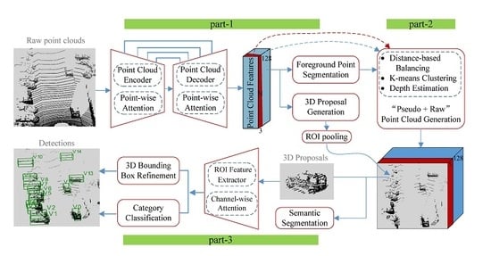
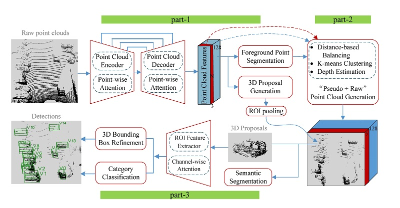
:In this paper, we propose a novel 3D object detector KDA3D, which achieves high-precision and robust classification, segmentation, and localization with the help of key-point densification and multi-attention guidance. The proposed end-to-end neural network architecture takes LIDAR point clouds as the main inputs that can be optionally complemented by RGB images. It consists of three parts: part-1 segments 3D foreground points and generates reliable proposals; part-2 (optional) enhances point cloud density and reconstructs the more compact full-point feature map; part-3 refines 3D bounding boxes and adds semantic segmentation as extra supervision. Our designed lightweight point-wise and channel-wise attention modules can adaptively strengthen the “skeleton” and “distinctiveness” point-features to help feature learning networks capture more representative or finer patterns. The proposed key-point densification component can generate pseudo-point clouds containing target information from monocular images through the distance preference strategy and K-means clustering so as to balance the density distribution and enrich sparse features. Extensive experiments on the KITTI and nuScenes 3D object detection benchmarks show that our KDA3D produces state-of-the-art results while running in near real-time with a low memory footprint.
1. Introduction
Three-dimensional (3D) object detection plays an important role in perception systems for autonomous driving. It helps users/systems to understand objects’ status for planning future motion safely by predicting 3D bounding boxes and class labels of objects in the scene. With the popularity of sensors deployed on mobile devices, more types of environmental information are captured and processed, which benefits accurate and robust detection in complicated driving scenarios.
Two-dimensional (2D) RGB images from cameras have rich texture descriptions and detailed semantic information but lack accurate depth information, which severely affects the precision of 3D bounding box estimation, even with stereo vision and prior knowledge of vehicle dimensions. 3D point clouds generated by light detection and ranging (LIDAR) are robust against illumination changes and can provide more spatial and structural information, including precise depth and relative location, which are the most representative formats of 3D sensor data. At present, many more algorithms rely heavily on point clouds and have been shown to achieve significant performance gains over image-based methods.
Challenges. Unlike images, point clouds are unordered, unstructured, and sparse. Typical convolutional neural network (CNN) architectures are inefficient when directly applied on such 3D data. In addition, the density and other attributes of points are highly variable across different distances and locations, whereas features learned in dense data may not generalize to sparsely sampled samples. For a similar reason, models trained with a common 3D scanner may not recognize fine structures, whereas a LIDAR with 64 or 128 rotating laser beams is expensive. Therefore, the following open challenges remain: how to effectively extract features from irregular and sparse points, how to make point clouds of objects not only meet density requirements but also retain their geometric shapes, and how to increase the point clouds-based network generalizability.
Our Contribution. In this paper, to address the aforementioned challenges, we present a robust and accurate 3D object detector called KDA3D (key-point densification and multi-attention guidance for 3D object detection), which takes point clouds as the main input, optionally adds images as a complement, and conducts detection and segmentation jointly within a single end-to-end learnable architecture. Figure 1 shows an overview of KDA3D’s three parts. Part-1 is a 3D foreground segmentation and proposal generation subnet. It first applies the encoder-decoder style full-point feature extractor on input point clouds to capture point-wise geometry features, and then appends specific heads on the generated feature map for foreground-point scoring and coarse 3D bounding box estimation. Compared with previous work using PointNet++ [1] as the feature extractor, we design a novel module called point-wise attention (PA) and embed it in each hierarchy of the whole extractor. PA module, as a point-feature selector, reweights each downsampled and upsampled point (associated features) by explicitly modeling the interdependencies between points, to further emphasize the “skeleton” point-features along a spatial dimension. Such a strategy allows representative points to get enough attention even in occlusion and clutter scenes.
Our part-2 is a key-point densification subnet, which implicitly uses color and texture to “supplement” the geometric information for constructing intensive and targeted point-feature representations. First, adopting the distance preference strategy to select 3D key-points from foreground points produced by part-1, and then using them as “seeds” to search related information in the image to generate “pseudo-point clouds” fitting target geometry. Finally, the “pseudo + raw” points and corresponding features are optimized to build a compact enhanced full-point feature map. Such strategies augment the objects’ geometric structure point-features while trying to solve nonuniform density sampling. This part could be selectively adopted by the networks according to their requirements and equipped sensors, taken as a low-cost solution to increase their generalizability and accuracy.
Our part-3 is a 3D semantic segmentation and box refinement subnet. It first conducts region pooling on the renewed full-point feature map based on 3D proposals from part-1. The pooled regions are then further semantically segmented, while aggregated by the region of interest (ROI) feature extractor for category classification and bounding box refinement. Our novelty is integrating another designed attention module called channel-wise attention (CA) into this region feature extractor. CA module, as a channel-feature selector, recalibrates per-channel features to emphasize the “discriminative” information along a channel dimension. Such a strategy helps the extractor capture finer geometry details in the ROI.
Our main contributions are summarized as follows:
- We propose a novel key-point densification component that generates targeted pseudo-point clouds from monocular images through the distance preference strategy and K-means clustering and uses the sorting simplification strategy to rebuild full-point feature map. It aims to supplement sparse target information and balance the density distribution, which is beneficial for detecting small or distant objects. Moreover, it reduces the algorithms’ dependence on the number of LIDAR sampling beams and enhances the applicability and consistency of point cloud features.
- We design multiple attention modules, called point-wise attention (PA) and channel-wise attention (CA), which are respectively incorporated into the full-point and ROI feature extractors with negligible overheads. They adaptively strengthen the “skeleton”/“distinctiveness” point-features to increase representation power of the network by exploiting the interpoint/interchannel relationship of features.
- Inspired by PointRCNN [2], we introduced foreground segmentation and semantic segmentation pipelines in succession to build a multi-task network, allowing the constraints added by fine segmentation to supervise and assist 3D bounding box regression for mutual benefit.
2. Related Work
Our work is inspired by the recent progress in 3D object detection from point clouds and images. In this section, we briefly review related work for LIDAR-only and joint LIDAR-camera data.
2.1. LIDAR-Based Methods for 3D Object Detection
2.1.1. Converting Point Clouds into Other Formats
To deploy typical CNN architectures on unordered and unstructured point sets for 3D recognition, many existing works [5,6,7,8,9,10,11] proposed various ways to convert 3D point clouds into regular representations before feature learning. VoxelNet [5] divides the 3D space into volumetric grids and groups the points based on them. Then, many voxel feature encoding (VFE) layers are stacked to extract voxelwise features, which are converted into dense 3D tensors. 3D CNNs are applied to process these tensors to generate 3D boxes. However, this state-of-the-art approach is difficult to use for real-time applications because of the high computational cost of 3D convolutions and the sparsity of volumetric representation. SECOND [6] improves [5] by applying sparse convolution instead of 3D CNNs (to reduce the computational cost) and introduces a novel angle loss (to improve the orientation regression). Part-A2 [10] also adopts 3D sparse convolution to extract sparse voxel-wise features from the point clouds. It uses the intraobject part information to learn discriminative 3D features and proposes the ROI-aware pooling to effectively aggregate the part features. PointPillar [11] explores pillar shape instead of voxel design to aggregate point-wise features and uses pseudo-images as the representation after voxelization. Further optimized towards speed, the model achieves 62 Hz.
In addition to the 3D voxel-grid form, VeloFCN [7] projects the point cloud to the front view (FV) and obtains a 2D depth and intensity image, which is processed by a fully convolutional network; the obtained convolutional feature maps are used to densely predict 3D boxes. PIXOR [8] projects and discretizes point clouds to specific height-encoded bird’s eye view (BEV); it uses a fine-tuned RetinaNet [12] to learn the view-features for real-time 3D object detection. Complex-YOLO [9] converts point clouds into a BEV representation with six channels; it uses a YOLO [13] network and a complex angle encoding to detect 3D objects with a high frame-rate and accurate orientation.
Advanced 2D detection frameworks or 3D (sparse) CNN can be readily applied to these data representation transformations. However, these quantization and projection operations obscure invariances and natural 3D patterns of raw point cloud input, even resulting in the loss of crucial and discriminative geometric details.
2.1.2. Using Raw Point Cloud
Recently, research has increasingly focused on learning 3D representations directly from raw point clouds without converting them to other formats. PointNet [14] as the pioneer employs a CNN-based architecture with T-Net networks and symmetric functions to encode and aggregate raw inputs for 3D object classification and semantic segmentation. PointNet++ [1] extends [14] using a hierarchical neural network to capture local geometric details. Against nonuniform sampling density, MSG and MRG are designed to group local regions and combine features from different scales. PointCNN [15] proposed an X-Conv operator that weights and permutes input points and features based on spatially local correlation in the point clouds. PointRCNN [2] extends [1] for 3D object detection. First, 3D bounding box proposals are generated in a bottom-up scheme, assisted by foreground point segmentation; then, canonical 3D box refinement is done. STD [16] tries to take advantage of both point-based and voxel-based methods. It extends [2] by proposing a PointsPool layer for converting features from sparse to dense representations in order to better refine proposals. 3DSSD [17], as a point-based 3D single-stage object detector, includes a candidate generation layer and an anchor-free regression head with a 3D center-ness assignment strategy and proposes a fusion sampling strategy, achieving a good balance between accuracy and efficiency.
These approaches have been shown to perform well. However, they suffer when dealing with far or small objects due to the limitations of point clouds (such as sparseness, nonuniform distribution, and only geometric spatial information).
2.2. Joint LIDAR and Camera Methods for 3D Object Detection
2.2.1. 3D-Driven 3D Object Detection
A few works have tried to exploit dense 2D RGB images to “complement” low-resolution point clouds for enriching learnable data. F-PointNet [18] first generates 2D bounding box proposals from images using a typical 2D detector and projects them into 3D space to obtain frustum regions. After selecting the corresponding local point clouds within frustums, cascaded PointNet [14] pipelines are applied to segment foreground points and estimate the 3D bounding boxes. RoarNet [19] extended [18] by deriving more geometrically feasible proposal locations by using 2D detection results from images to reduce sensors out of synchronization problems. Then using variants of PointNet [14] to learn the cropped 3D points within standing cylinders for 3D bounding boxes estimation. F-ConvNet [20] improves [18] by producing a sequence of frustums for each region proposal instead of only one. Then, multiple [14] pipelines process corresponding region-points to generate frustum-level features, which are reformed to be used for 3D bounding boxes regression by the fully convolutional network.
These cascade patterns, which are not end-to-end learning, cannot perform joint reasoning over multimodal data, and their performance is bounded by the 2D detection step using images only.
2.2.2. Multi-View Fusion Networks
Compared with 2D-driven and cascade methods, some studies aim at fusing the two modalities more thoroughly. MV3D [21] transforms point clouds into the BEV and FV, where the image is processed separately to generate multiple-view feature maps. It extends the image-based RPN of Faster R-CNN [22] to 3D for generating proposals from the BEV feature maps. Then, it projects the proposals onto the corresponding feature maps to crop view-specific region features, which are combined by a deep fusion scheme for the final 3D detection. AVOD [23] first uses a modified VGG-16 [24] to generate full-resolution feature maps from images and BEVs. Then, it improves [21] that fusing anchor features from multiple feature maps in the RPN phase, which obtains reliable proposals for smaller classes. ContFusion [25] uses continuous convolutions to encode accurate dense geometric relationships between two modalities, to fuse image and BEV features at different resolution levels, which is helpful for 3D object detection. However, the fusion methods above are usually applied at a coarse level with significant resolution loss, and overall level fusions are prone to redundant data and are time-consuming. MMF [26] fuses information from point clouds, images, and maps to accomplish multiple tasks including 2D and 3D object detection, ground estimation, and depth completion. These tasks benefit each other and enhance final performance on 3D object detection. PI-RCNN [27] fuses multi-sensor features directly on 3D points. It uses point-wise continuous convolution and additionally adds a Point-Pooling and an Attentive Aggregation to obtain better fusion performance.
In this paper, referring to the above [1,2,23,25], our method adopts two-stage architecture for 3D object detection and segmentation. We design an image-based density enhancement method to improve the sparsity and nonuniformity of point clouds and introduce the self-attention mechanism to emphasize crucial features and suppress useless ones. Moreover, we incorporate several improvements to achieve better performances.
3. KDA3D Architecture
The main idea behind KDA3D is to construct a multi-task network that embeds the multi-attention modules and the pseudo-point cloud generator to accurately detect and segment 3D objects. The overall structure is illustrated in Figure 1 and consists of three parts: (1) a 3D foreground segmentation and proposal generation subnet, (2) a key-point densification subnet, and (3) a 3D semantic segmentation and box refinement subnet.
3.1. 3D Foreground Segmentation and Proposal Generation
Inspired by state-of-the-art 2D [22,28,29] and 3D [2,30] object detectors, our part-1 aims to accomplish the following tasks. First, we design the full-point feature extractor to learn geometry information from raw point clouds under attention guidance. Second, each point of the whole scene is scored to segment foreground points based on learned features. Third, 3D region proposals with high recall and relatively low precision are generated through the segmentation results.
3.1.1. Full-Point Feature Extractor
PointNet series [1,14,18] are pioneering efforts that directly process raw point clouds. PointNet++ [1] is used as a backbone network by several architectures [2,18,31,32] to extract point-wise features. However, the problem of imbalance between the number of noninformative and informative points in the input sets has not been fully considered in these works. Specifically, at each level of the [1] hierarchical structure, the max/average pooling is often used to aggregate information. Although this encoding method is efficient and practical, the critical but relatively less information would be progressively “diluted” along the hierarchy, which is difficult to compensate by upsampling and skip-connections. Our intuition is to allow the feature learning networks to decide how much each point and its features (sampled and extracted at the previous hierarchy) should contribute to the next hierarchy according to the local context and global semantic information of points. The goal is to increase the proportion of useful points (features) in the final feature map.
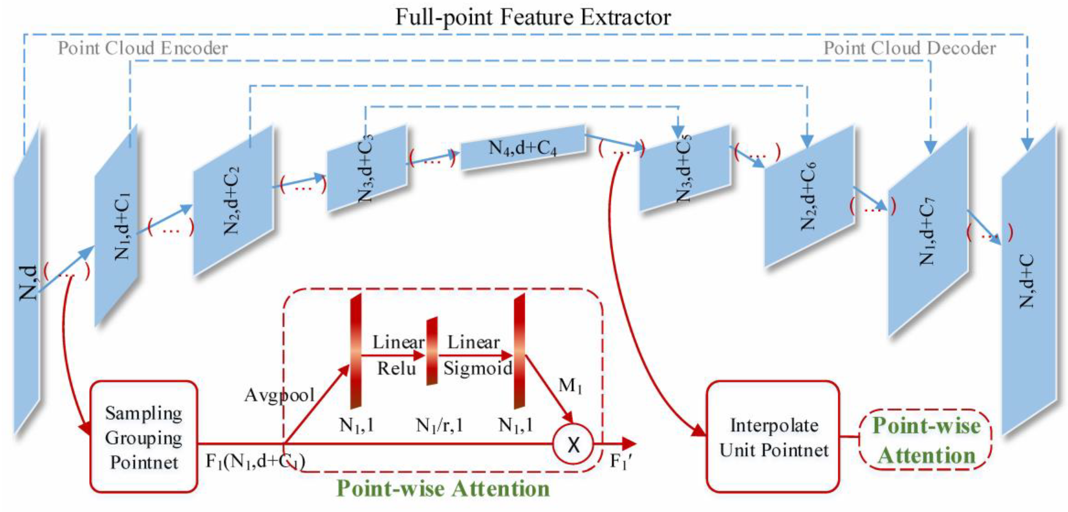
Therefore, inspired by [33,34,35,36], we propose an effective attention module named point-wise attention (PA). Most self-attention mechanism works, such as channel-wise [33] and spatial [36] attention, were developed for image-based CNNs. Compared with these, our attention modules are designed for 3D point clouds, efficiently helping the information flow within the network by learning which information to emphasize or suppress. As shown in Figure 2, we use the PointNet++ [1] with multi-scale grouping (MSG) as our basic backbone network, which is composed of a number of set abstraction (feature propagation) layers for encoding (decoding). We incorporate the PA module into its every hierarchy to construct our full-point feature extractor.
For example, the first level of the encoder has four key steps: sampling layer, grouping layer, mini-PointNet, and PA module. As shown in Figure 2, let be an input matrix for points wsup;ith -dim coordinates. After the first three steps, outputting matrix of subsampled points with -dim coordinates and -dim new feature vectors summarizing the local context. In the fourth step, is fed to our PA module, which exploits the interpoint relationship of to infer the point attention map . is a collection of per-point modulation weights for reweighting each point (the corresponding feature) of . We describe this operation below.
First, is aggregated across its coordinate and feature dimensions by using a global average pooling operation, generating a point descriptor: , which is then forwarded to the multilayer perceptron (MLP) to produce our point attention map . To limit module complexity and aid generalization, the MLP consists of two small fully connected (FC) layers around the nonlinearity. The first FC activation size was set to followed by a ReLU [37]. The second FC has an activation size of followed by a sigmoid, where is the reduction ratio. Finally, the element-wise multiplication operation is used to process and obtain the final refined output . In short, our PA module is computed as:
where and denote the sigmoid and ReLU activation functions, respectively; and refer to the MLP weights; denotes the element-wise multiplication operation. The PA module can be seamlessly integrated into several architectures and jointly trained with other parts in an end-to-end fashion; this only imposes a slight computational cost owing to its light weight.
As the hierarchy level of the encoding part deepens, the extracted features in each level are optimized by PA and passed to the next level. Then, features are further aggregated into larger units, until obtaining the strong semantic features of the whole point set. At the decoding part of level-wise interpolation and abstraction, features from subsampled points are progressively propagated to the original points along the hierarchy, which is accompanied by skipping connections, where the PA module of each level guides the restoration by suppressing useless ones in subsampled point features. This final output is of high resolution and strong-semantic and it is shared by the subsequent foreground point segmentation and 3D proposal generation tasks.
3.1.2. Foreground Point Segmentation
Foreground point segmentation can be considered an objectness classification for each point. On the one hand, this task promotes the full-point feature extractor to effectively capture contextual information by providing clear segmentation constraints and goals. On the other hand, it offers important support for simultaneous 3D proposal estimation and is a prerequisite for subsequent key-point densification. Inspired by [2], we append the segmentation head, which consists of two convolution layers, to the learned full-point feature map for estimating the foreground mask (scores). Because objects are naturally well-separated in 3D scenes, the ground-truth segmentation masks are provided by the annotated 3D bounding boxes in the training data. For training, we apply the focal loss function [12] to handle the class imbalance between the number of foreground points and the background points in a large-scale outdoor scene.
3.1.3. 3D Proposal Generation
We append the proposal regression head for preliminary detection. It is performed simultaneously with the above segmentation head to jointly generate 3D proposals with higher recall. As in 2D and 3D two-stage detectors [2,5,22], a 3D proposal is encoded as in the camera coordinate system, where is its centroid, is the object dimensions, and is its orientation from the bird’s view. Following [2], the prior is sampled at the coordinates of the input points, which should come from ground-truth foreground points when training. The prior is determined by clustering the training samples for each class. This avoids using a large set of 3D predefined boxes and reduces the search space.
This regression head indirectly predicts , which represents the differences between the priors and the ground-truth bounding boxes. During training, we follow the bin-based regression losses of [2] to constrain the 3D proposal generation: for center location and orientation , we adopt cross-entropy loss for their bin classification and smooth L1 loss for the corresponding residual regression. For and size , we directly use smooth L1 loss for their regression. To remove the redundant proposals, we use 3D nonmaximum suppression (NMS), combined with the foreground segmentation results, at an intersection over union (IoU) threshold of 0.85/0.8 to keep the top 512/100 proposals for training/inference.
3.2. Key-Point Densification
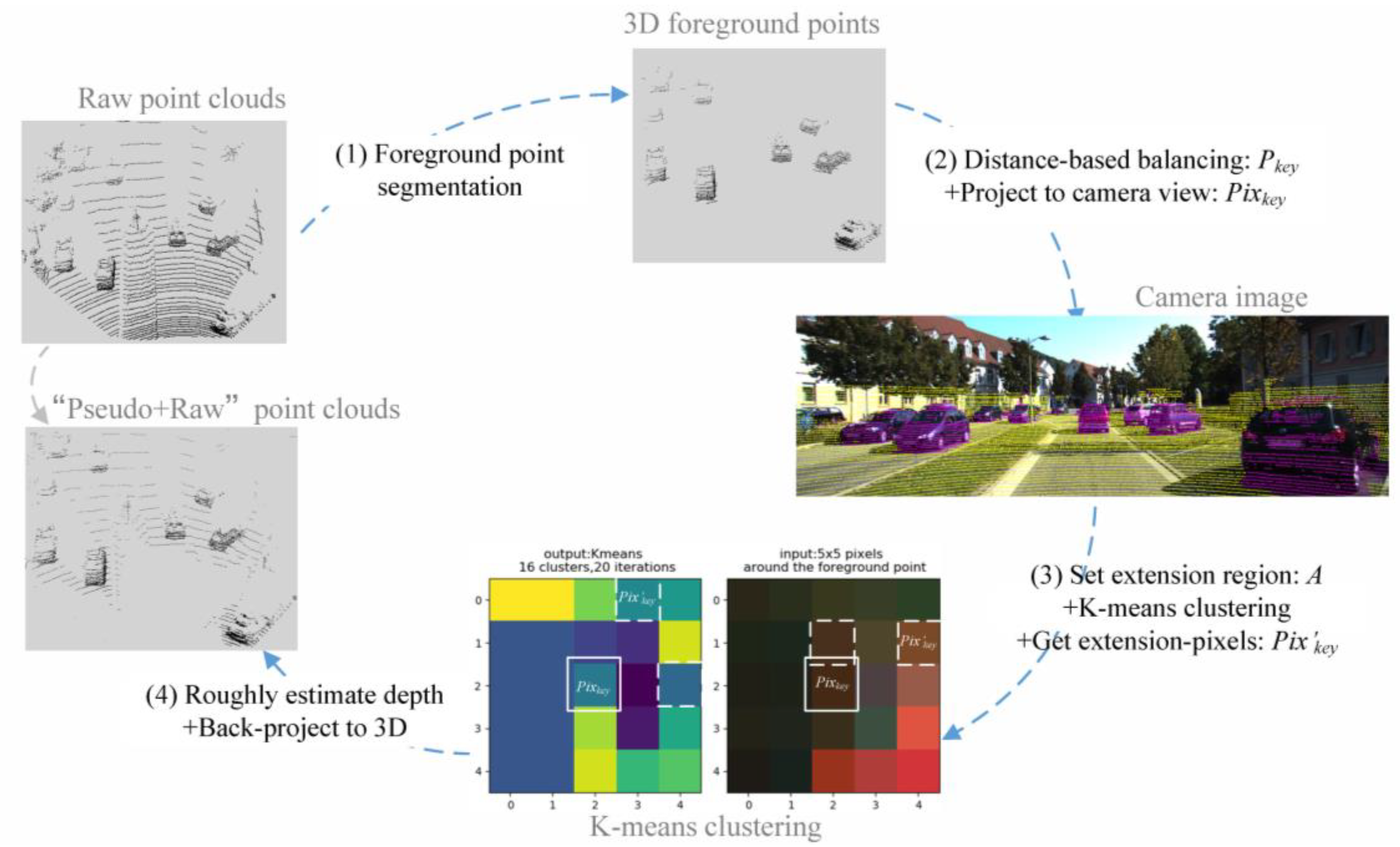
The quality of object point clouds is usually unstable, affected by laser beam number, spatial distance, and scene complexity, etc. It is difficult for data-driven algorithms to maintain consistent performance on sparse and variable inputs. Although PointNet++ proposes the MSG/MRG to adaptively learn features from regions of different scales, it is still affected by sparsity when balancing the target information. In this case, we propose the key-point densification component (our part-2), which aims to supplement target-related points (features), ease density variety, and assist in building a generalized and robust detection model. As shown in Figure 3, the component includes four steps: (1) distance-based balancing, (2) K-means clustering, (3) pseudo-point cloud generation, and (4) full-point feature reconstruction.
3.2.1. Distance-Based Balancing
The increase of nonobject points in point sets complicates feature extraction and leads to redundancy. Thus, density enhancement for point clouds should be selective and targeted rather than indiscriminate. In this case, we take the foreground points generated by part-1 as the candidate collection, which includes rich and relatively reliable object information, allowing selection of the “seeds” for follow-up precise augmentation. Intuitively, the easiest selection method is to use the objectness score of each point (foreground scores) from part-1 as criteria, i.e., “seeds” are determined by score sorting. Objectively, objects farther away from the sensor have relatively fewer points in the large outdoor scene. Considering that these points need to be more augmented but are prone to obtaining lower scores in part-1, we adopt the distance preference strategy combining scores to sample “seeds” (key-points) to augment target information while balancing the density nonuniformity. The operation is described below.
Given an input set , its corresponding foreground scores (normalized) are . The coordinate of each point is , and the distance to the sensor is , where . We set threshold to determine the key-points to be enhanced. As in (3) and (4), for the car class in KITTI, is considered to be a key point if its score is above 0.3; the supplementary condition is that if its distance is greater than (equal) 40 m, then just needs to be above 0.1. For the pedestrian and cyclist classes in KITTI, these score thresholds are reduced to 0.2 and 0.05.
3.2.2. K-means Clustering
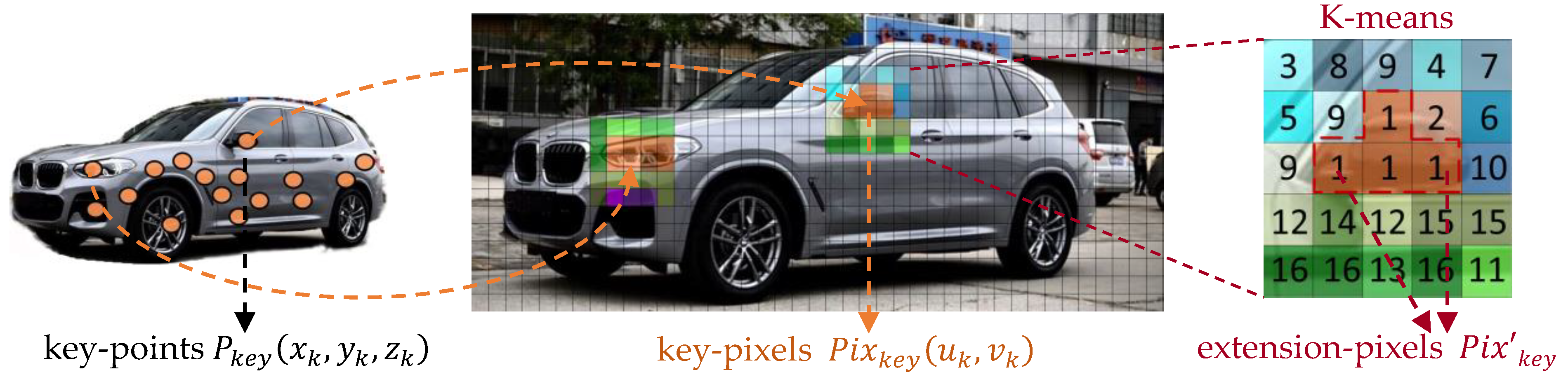
Unlike existing fusion methods [21,23,25] that explicitly use color and texture to “supplement” geometric information, we consider different attributes to be complementary and parallel when dealing with perception problems. Roughly or directly fusing them will confuse the network and cause difficulty in learning. Therefore, we try to implicitly convert useful information in RGB images into the form compatible and concordant with point cloud representations, which has not been done in previous related networks. As shown in Figure 1 and Figure 3, we first project the selected key-points onto the RGB image to obtain the corresponding key-pixels. Then, we cluster their neighborhoods to search for extension-pixels that are “close” to key-pixels. Next, we back-project extension-pixels to the 3D space to get target pseudo-point clouds that “fit” target geometrical shapes. We describe this procedure in the following paragraphs.
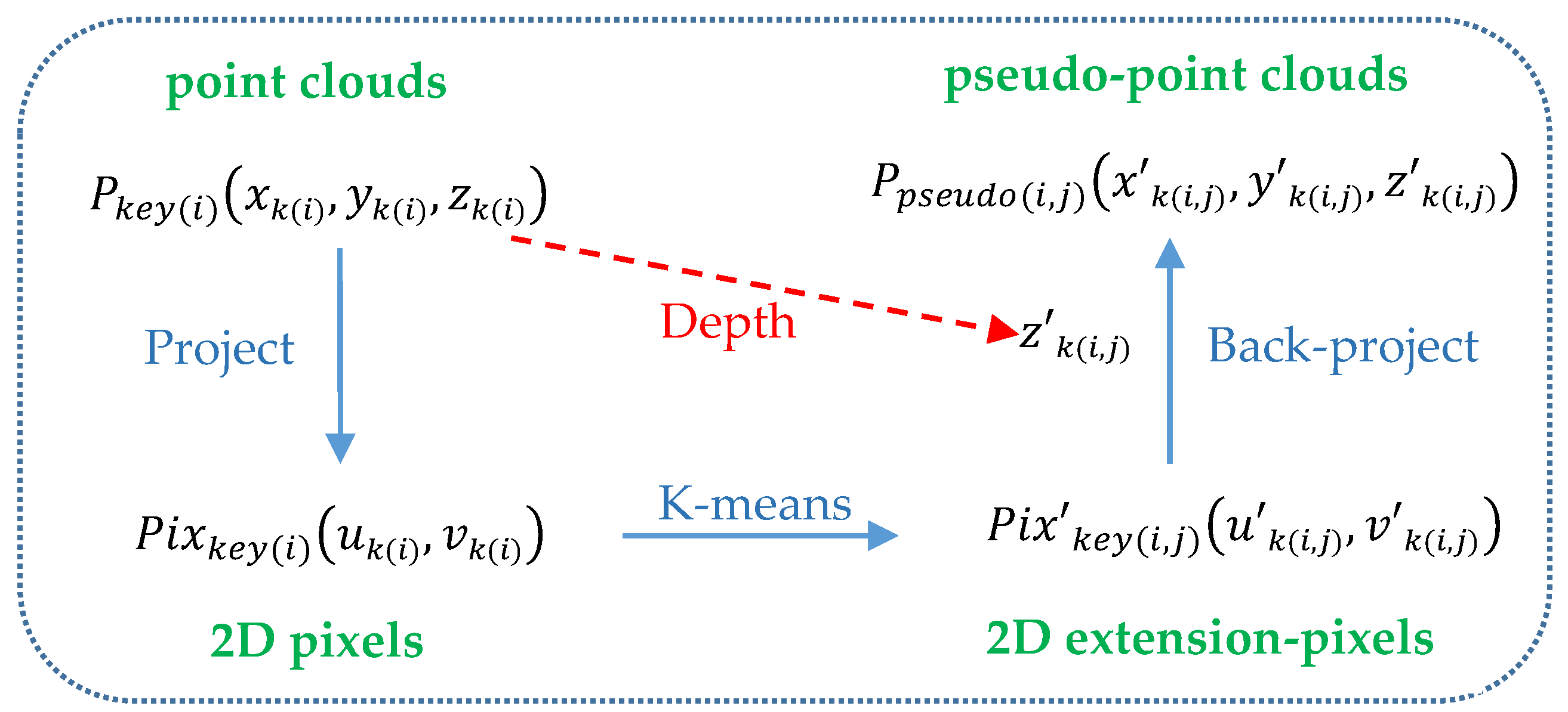
For a point set, given the key-points and their coordinates , which are first transformed from the 3D LIDAR coordinate system to the camera coordinate system and then projected onto the 2D camera image to obtain the corresponding key-pixels and their coordinates , the process is formulated as in (5) and (6).
where is the rigid-body transformation from the LIDAR coordinate system to the camera coordinate system, consists of a rotation matrix and translation vector . is a projection matrix that converts the 3D points in the camera coordinate system to the 2D pixels in the camera image. These calibration parameters are provided by the KITTI and nuScenes benchmark suite.
It is common for the resolution of LIDAR point clouds to be significantly lower than that of the corresponding camera image. Thus, the obtained key-pixels are sparsely distributed on the image and only occupy a small part of the total pixels. In such a case, as shown in Figure 4, we take each key-pixel as the center and combine it with surrounding pixels to build a target region of size, is determined as:
where is the number of processed point clouds, is the resolution of the corresponding image, and their values follow [2,3]. Intuitively, these divided regions can be viewed as the supply units for enriching the corresponding key-pixels.
For each region , we firstly use the simple but efficient K-means [38,39] algorithm to cluster the pixels within it according to color and texture. Then we extract pixels with the same category as the center pixel , called extension-pixels , which contain comparable or even more helpful information. For example, as shown in Figure 4, the rearview mirror has one key-pixel projected from the 3D key-point, after getting key-pixel’s region , we perform K-means algorithm to cluster the pixels in into 16 categories, where three pixels (in orange) in the same category as the key-pixel are the expansion pixels.
We randomly determine the initial cluster center; the numbers of clusters are set to 16 and 8 for car and pedestrian/cyclist classes; the clustering termination criteria is that the maximum number of iterations is 20 or the accuracy is 0.5. The number of searched extension-pixels based on each key-pixel is different, depending on how much efficient information is in its target region. It is flexible rather than fixed to avoid introducing useless information.
3.2.3. Pseudo-Point Cloud Generation
We back-project the resulting 2D extension-pixels into 3D space to obtain pseudo-point clouds, which are an effective complement to the original sparse point clouds, allowing useful parts (such as the rearview mirror and car lamp in Figure 4) to get more geometric details. The back-project procedure is shown in Figure 5: we first estimate the depth information of each pixel in . Because the size of is small, considering computational complexity, we assign a depth value of 3D key-point to the corresponding instead of using interpolation calculations. Specifically, for an extension-pixel , its corresponding key-pixel is . is projected from the key-point , so is specified to as the estimated depth of . Then we back-project into 3D space to obtain according to Equation (5) and Equation (6).
3.2.4. Full-Point Feature Reconstruction
The pseudo-point clouds generated based on foreground key-points contain rich geometric structure information transformed from the color and texture information of images. How to combine them with the corresponding raw point clouds (features) is a key issue. Both being directly added together will not only increase the computational complexity but also dilute the target information. However, just merging pseudo-point clouds and key-points (removing low-score points) may lose false-negative information and some remaining background points are beneficial for subsequent prediction. Thus, we use the sorting simplification strategy with the help of foreground scores to build an enhanced full-point feature map with sufficient target information and relatively low resolution.
The pseudocode of the sorting reconstruction procedure is shown in Figure 6. First, we reorganize the original point set to form the new set . is set to 8192, which is reduced by half compared to the point clouds used in part-1 to save computational resources for subsequent part-3. Second, we reconstruct the full-point feature map generated in part-1 according to the reorganized point set , obtaining the compact enhanced full-point feature map .
3.3. 3D Semantic Segmentation and Box Refinement
In part-3, we propose a 3D semantic segmentation and box refinement subnet, which aims at further optimizing and regressing the previously generated proposals to obtain the final detection results. First, we design a segmentation branch to assign semantic labels to points within each proposal. Second, we propose the ROI feature extractor to further learn the proposal features with the help of channel-attention modules. Third, these newly abstracted proposal features are fed to the two specific heads to perform 3D bounding box refinement and category classification, respectively.
3.3.1. 3D Semantic Segmentation
Given a 3D proposal generated in part-1, we first randomly sample points from the pooled region of , and then pool the corresponding features from the enhanced full-point feature map . Next, we append a simple segmentation head to canonical [2] to estimate the semantic mask. The head is composed of three convolution layers of 1 × 1 kernels, which aims to fit an optimal function that gives an accurate semantic label to each point within . Semantic segmentation can be considered as detailed descriptions of the geometric shape of objects, the internal mechanism of which is similar to fine location prediction. Believing that extra supervisions added by learning to segment objects are beneficial for 3D box refinement, our future work will be to replace the boundaries with segmentation results to provide more precise valid proposals. For training, consistent with the foreground point segmentation of part-1, we adopted the focal loss function [12]. The free-of-charge segmentation labels of raw point clouds are still given by 3D ground-truth box annotations, while those of pseudo-point clouds generated in part-2 need to be provided additionally. Thus, we assign the objectness labels to the corresponding pseudo-points for creating pseudo-annotations when performing depth estimation for extension-pixels, which further explores the abundant information in annotations.
3.3.2. ROI Feature Extractor
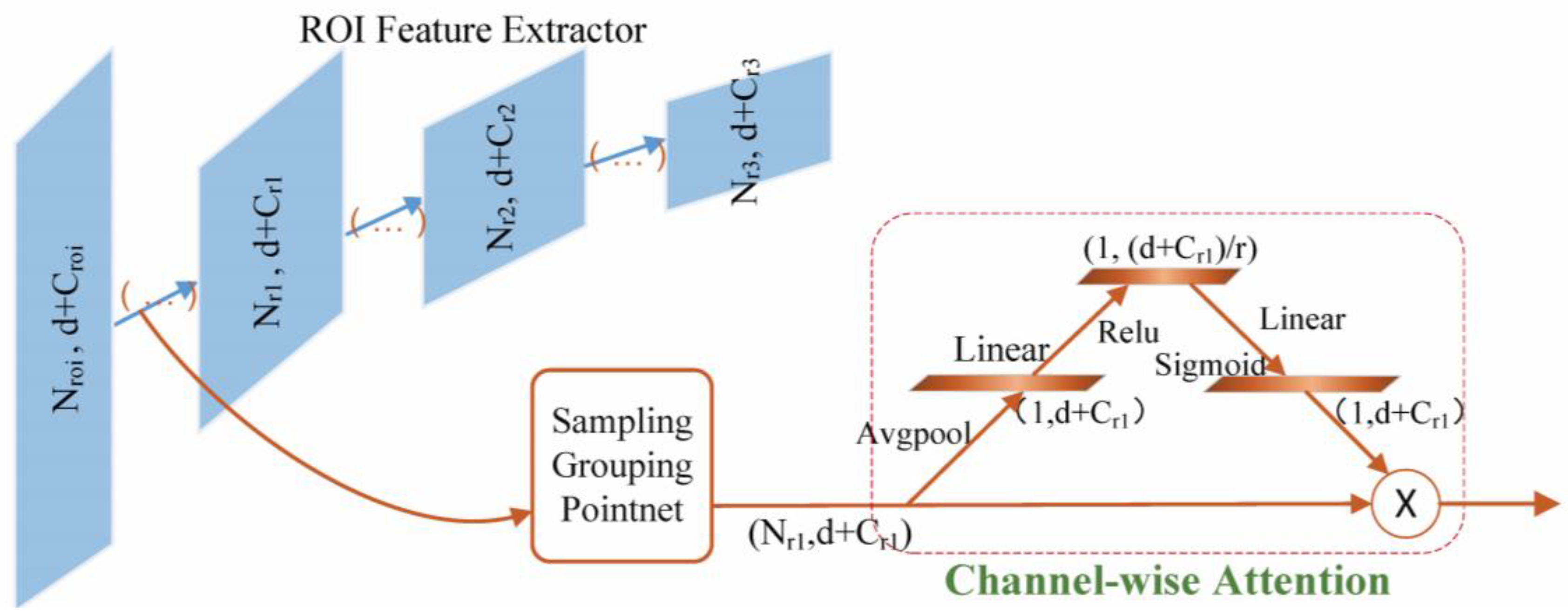
We design specific feature learning networks for the tasks of our different parts. The full-point feature extractor (see Section 3.1.1) aims to produce representative point-wise features for achieving robust primary detection. The ROI feature extractor, in this section, is designed to capture finer geometric structures for high-quality 3D bounding box regression. As shown in Figure 7, we adopt the structure of [1], which is similar to the encoding part of our full-point feature extractor. Three set-abstraction levels with single-scale grouping are used to aggregate and abstract proposal features, where subsampled point groups are , , . A single feature vector is finally generated for category classification and proposal location refinement. To better extract discriminative points (features) in the ROI, inspired by [33], we propose a second attention module called channel-wise attention (CA), which is flexibly incorporated into each hierarchy of the ROI feature extractor to progressively guide and reinforce the learning process.
Compared to the point-wise attention module (see Section 3.1.1), the CA module models dynamic and nonlinear dependencies between channels, rather than points, using global information of the ROI. As shown in Figure 7, CA squeezes the spatial dimension of the input features to compute the channel attention. Specifically, given proposal features , we get after sampling, grouping, and mini-PointNet. First, is aggregated across its 1D spatial dimensions using a global average pooling operation, producing the channel descriptor . Next, is forwarded to the MLP with two FC layers and activation functions: a dimensionality-reduction layer , where is the reduction ratio, a ReLU, and then a dimensionality-increasing layer , a sigmoid. Finally, the channel attention map is obtained, , which is the collection of per-channel modulation weights. Element-wise multiplying and to obtain the optimized output .
CA emphasizes discriminative and salient information through reweighting per-channel features of ROI. By recursively applying CA modules, our ROI feature extractor adequately captures the context of points and effectively responds to useful details to output high-quality object description, which is beneficial for the following confidence classification and box refinement.
3.3.3. Generating Final Detections
The newly extracted proposal features are fed to the two specific heads, which both consist of three convolution layers, to perform oriented box refinement and category classification for each proposal. Similar to the 3D proposal generation of part-1, a 3D bounding box is represented with a 7-dimensional vector . The corresponding regression value is indirectly computed by this regression head. We apply the bin-based regression losses from [2] for regression tasks of the bounding box location, dimension, and orientation vector, and use a cross-entropy loss for the classification task. To remove overlapping detections, NMS is used with an oriented 3D IoU threshold of 0.1.
4. Experimental Results and Discussion
We evaluate our proposed KDA3D on the widely used KITTI object detection benchmark (our experimental evaluation on nuScenes dataset can be seen in Appendix A). First, we briefly introduce the experimental setup and implementation details. Second, we demonstrate the main results of our method by comparing with state-of-the-art 3D detection methods. Third, extensive ablation studies are also performed to validate the effectiveness of individual components in our method. Finally, we present qualitative results and discuss future directions.
4.1. Experimental Setup
4.1.1. Datasets and Evaluation Metric
The KITTI dataset contains 7481 point clouds/RGB images for training and 7518 for testing. Because the ground-truth for the test set is unavailable and access to the test server is limited, we follow the protocol described in [2,30,40,41] to split the original 7481 training frames into the new train set and validation (val) set, adopting approximately a 1:1 ratio. We conduct our experiments using this splitting, where all models are trained on the train set and evaluated on the val set.
We follow the official KITTI protocol, evaluating both 3D and BEV object detection tasks at a 0.7 IoU threshold for the car class and 0.5 IoU thresholds for the pedestrian and cyclist classes. Their evaluation results are given in terms of the average precision (AP) metric. In this section, we use and to denote AP for the 3D and BEV tasks, respectively. We evaluate 3D proposal generation using 3D box recall, where the 3D IoU threshold is 0.5. For each category, detection results are evaluated based on three difficulty levels: “Easy”, “Moderate”, and “Hard” considering the object size, distance, occlusion, and truncation. The runtime refers to the inference time of our network for per-scene/image on a Titan Xp GPU.
4.1.2. Training Details
We train two network versions: KDA3D and KDA3D (slim). KDA3D, as described in this paper, consists of three parts and uses both point clouds and images. KDA3D (slim) does not integrate the key-point densification component (part-2), it is a simplified version that only exploits point clouds. Moreover, for the KITTI dataset, we train two separate networks for each version: one for car class and one for pedestrian and cyclist classes. Our networks are trained in two steps:
- In the first step, we only train the 3D foreground segmentation and proposal generation subnet (part-1). The first step is trained for 200 epochs with a batch size of 16 without a pretrained model. The prior boxes are considered in the evaluation (computation) of the regression loss only if they are generated from ground-truth foreground points, which are inside the 3D ground-truth boxes.
- In the second step, we lock the parameters of part-1 to the results trained in the first step. We only update parameters of the 3D semantic segmentation and box refinement subnet (part-3). Part-2 of KDA3D participates in training to ensure running integrity, but its parameters do not need to be updated. The second step is trained for 70 epochs, batch size 4 with 256 proposals, and approximately 50% of the proposals are kept positive. Whether the proposals are considered as positive, negative, or ignored samples for training relies on the IoUs between them and all the ground-truth boxes. Detailed descriptions of the IoU thresholds for car and pedestrian/cyclist classes are given in Table 1. Taking the car class as an example, for the classification task, a proposal is considered positive if its maximum 3D IoU is above 0.6. It is treated as negative if its maximum 3D IoU is below 0.45. For the box regression task, we set 3D IoU 0.55 as the minimum threshold.
The above two training steps have the following settings: we use Adam optimizer [42] with an initial learning rate of 0.002, which decays exponentially every 50 epochs with a decay factor of 0.5. We train the KDA3D/KDA3D (slim) network using a single Titan Xp GPU took 15/13 h.
4.2. Main Results and Comparison with State-of-the-Arts on KITTI Benchmark
Comparison with State-of-the-Art Methods. We evaluate and compare two versions of our implementation (introduced in Section 4.1). “Ours” refers to KDA3D and “Ours (slim)” refers to KDA3D (slim). Table 2 presents the results of our methods on the 3D detection benchmark and the BEV detection (3D location) benchmark of the KITTI val set, compared with several state-of-the-art algorithms, including LIDAR-based [2,5,6] and joint LIDAR-camera [18,21,23,25] methods. MV3D [21] uses a pretrained model for initialization. F-PointNet [18] uses a 2D detector that has been fine-tuned using ImageNet [43] weights. SECOND [6] and PointRCNN [2] use the ground-truth augmentation approach, whereas our networks are trained from scratch and with no further enhancements except standard data flipping and scaling. Notably, relatively fewer current methods publicly provide detection results for the pedestrian and cyclist classes. Hence, more comparisons of the car class are presented in Table 2.
In Table 2, we observe that even with only the LIDAR data, Ours (slim) performs reasonably effectively on all three classes, being superior to most point clouds-based methods. Moreover, once we add our key-point densification (part-2), Ours using multimodal data performs quite well. Specifically, for the car class, Ours scores above all other methods on “Moderate” and “Hard” instances in 3D and BEV object detection, with noticeable margins of 1.08% AP3D and 4.5% APBEV on “Hard” instances in comparison with the second-best method. It indicates that Ours has an advantage when dealing with highly occluded or far objects in complex scenarios. For the pedestrian class, Ours scores significantly outperforming Ours (slim) and VoxelNet [5] in BEV object detection, demonstrating that using multimodal descriptions is conducive to improve location precision. For the cyclist class, Ours is top-performing except for scores slightly lower than F-PointNet [18] on the “Easy” instances in BEV. In fact, the number of cyclist instances in the KITTI dataset is the smallest, which proves that our network has a powerful and robust learning ability to grasp nuances of different object shapes from limited samples.
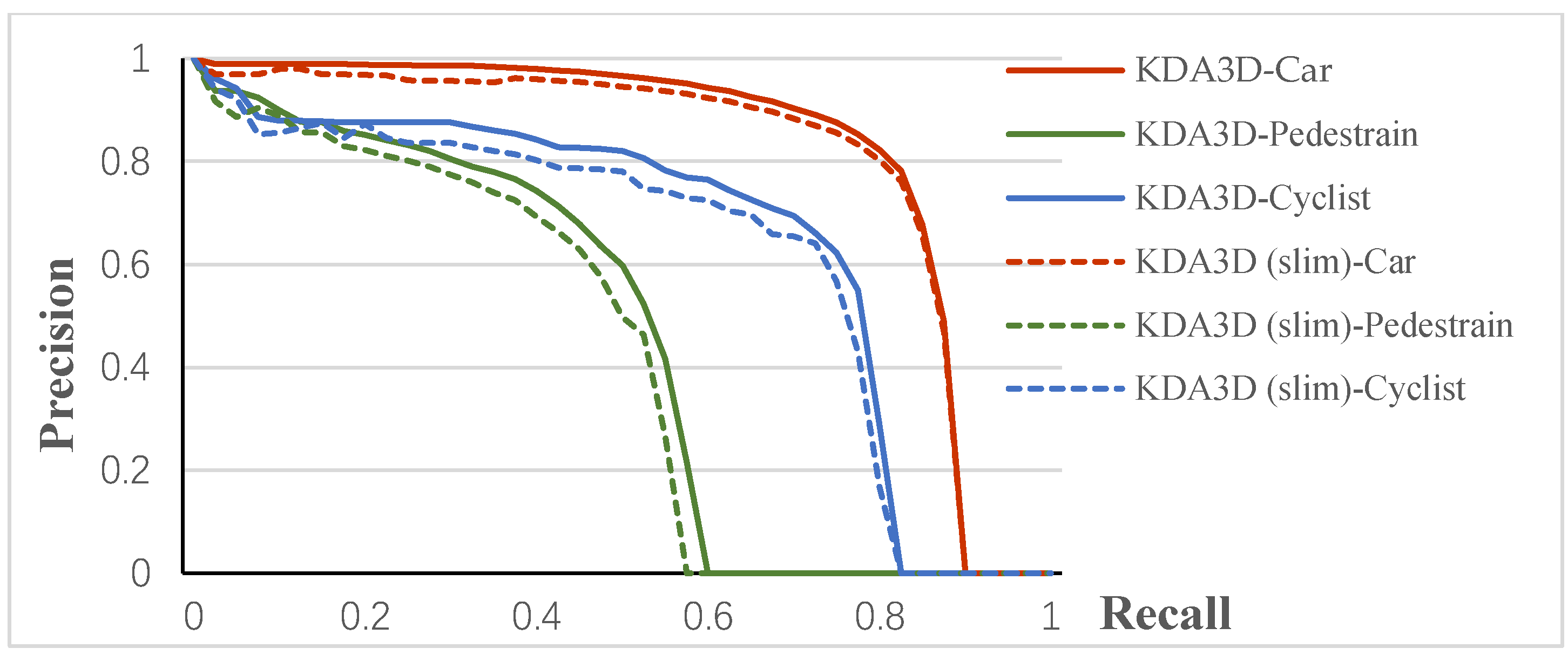
PR Curve. Figure 8 shows the precision-recall curves of KDA3D and KDA3D (slim) for 3D object detection. It can be seen that the two network versions perform well in all three classes, and as expected, KDA3D has higher average precision.
Inference Time. Concerning the inference times of our networks for one frame on a Titan Xp GPU (and a single CPU core) shown in Table 2, our runtimes are slightly longer than of the fastest method, but we still achieve comparable speeds. Specifically, for KDA3D (slim): the full-point feature extraction takes 55 ms; parallel foreground point segmentation branch and proposal generation branch (including NMS) take 13 ms; parallel semantic segmentation branch and ROI feature extractor take 20 ms; parallel category classification branch and box refinement branch take 12 ms. For KDA3D: in addition to the above spending, its key-point densification component takes 30 ms or 20 ms (for car or pedestrian/cyclist class).
Overall, Ours (slim) performs well in 3D and BEV object detection with a fast inference speed; Ours can produce higher-accuracy results, especially for objects with less appearance information such as small, far, and occluded objects. The outputs of our networks are visualized in Section 4.4 and Appendix B.2, where we observe accurate 3D box predictions even for challenging cases.
4.3. Ablation Studies
4.3.1. Effect of Key-Point Densification Component
In contrast to most multi-sensor-based algorithms that repeatedly fuse multimodalities in multiple stages, our proposed key-point densification component (part-2) is plug-and-play with few modifications to other parts, which flexibly and conveniently enhances target information (see Section 3.2). The component adopts the high-efficiency K-means algorithm for clustering and does not require training and updating parameters. Hence, its adopted strategies and prior designs are the main factors determining its performance.
In the first half of Table 3, we evaluate the impact of adopting different key-point selection strategies for density enhancement. We take KDA3D (slim) without part-2 as the basic network (the first row of Table 3). For the second row of Table 3, we enhance all input points (N = 16,384) to overcome the sparseness of the point set. However, it only produces a slight increase compared to the basic network. For the third row of Table 3, we only enhance the points with foreground scores above 0.2/0.3 obtained in part-1, which brings a clear performance improvement, especially on the “Moderate” instances, with gains of 1.01%, 3.07%, and 1.65% for the car, pedestrian, and cyclist classes. This verifies our assumption that the pseudo-point clouds generated from monocular images can effectively densify the original point set for better prediction, but indiscriminate processing would introduce noise, reducing the enhancing effect. For the fourth row of Table 3, we adopt the proposed distance preference strategy to select the key-points. As expected, the version with distance considerations gets generally higher than that solely using foreground scores, especially on the “Hard” instances. This shows that it is feasible to use algorithms to compensate for the limitation of hardware detection distance.
In the second half of Table 3, we study how to combine “raw + pseudo” points and corresponding features. For the second to fourth rows of Table 3, we add the raw and pseudo point clouds (features) together directly. For the fifth rows of Table 3, we only merge generated pseudo and selected foreground points (features), that is, only ones considered to be target are retained while others are cut. For the sixth rows of Table 3, we use the proposed sorting simplification strategy to reconstruct pseudo and raw points (features) according to foreground scores. The results show that the “compact” version obtains the best effects, general scoring slightly above the “add” version while greatly reducing the computational overhead, and the “cut” version performs significantly worse. This phenomenon can be attributed to the fact that proper foreground and background ratios help the network to understand features, while excessive use of prior knowledge to emphasize target information is not necessarily conducive to detection (as described in Section 3.2.4).
Table 4 shows the effect of varying K-means parameters on the runtime and AP3D of our KDA3D. In this experiment, we only focus on the most important “Moderate” instances for all three classes, which are the closest to the real situations. In our method, the smaller number of clusters, the more extension-pixels are obtained. However, it will lead to an increase in false positives and reduce fit between the resulting pseudo-point clouds and object geometries. Therefore, we need to find a compromise between the quality and quantity of object descriptions. Rows 1–3 of Table 4 present the results for conducting 20 iterations with 4, 8, and 16 clusters, respectively. One can see that setting 16 clusters achieves relatively good performance with the least parameters overhead. For the fourth row of Table 4, we increase the number of iterations to 40 based on the setting of the third row, which provides a slight improvement for the cyclist class but adds much computational cost.
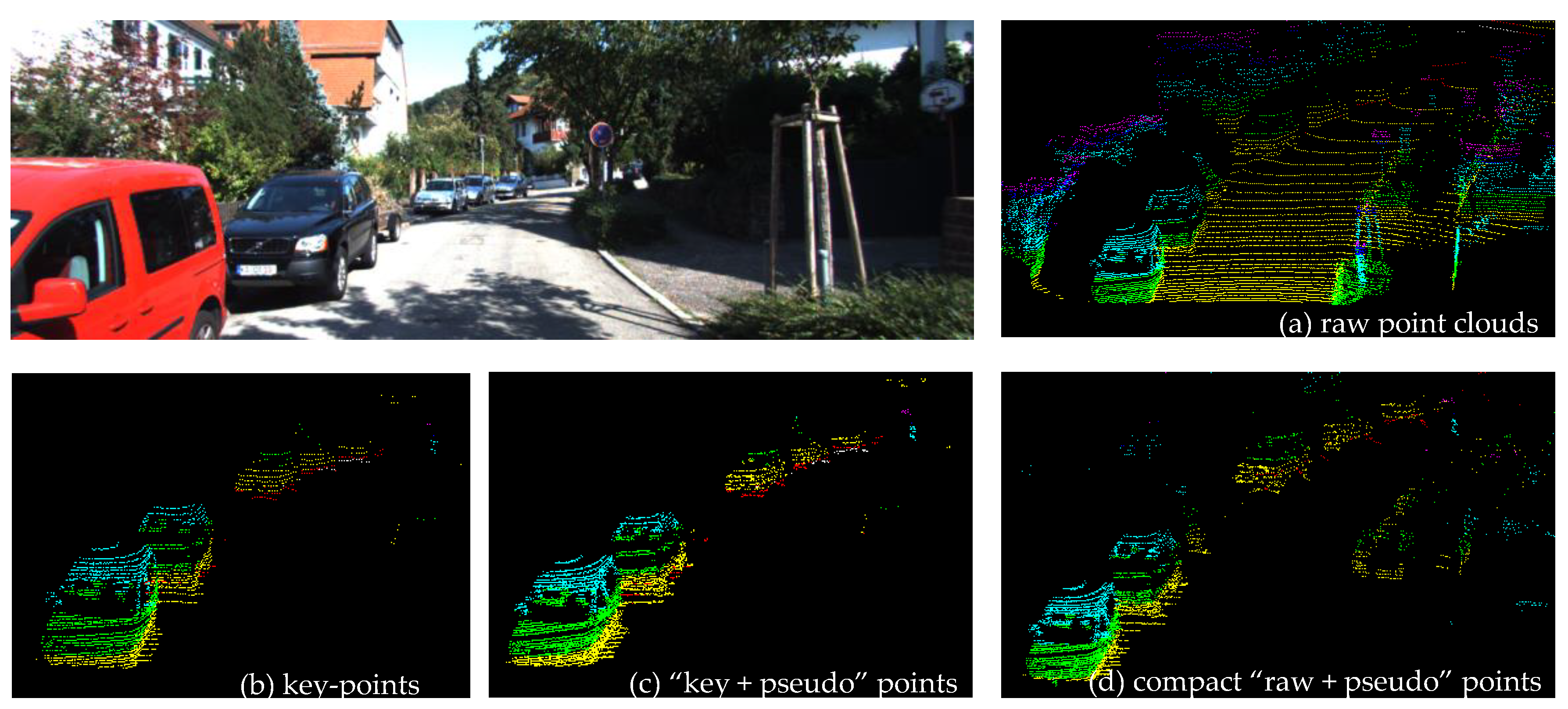
Figure 9 visualizes the results of the key-point densification. Figure 9b demonstrates that key-points selected through the distance preference strategy are representative and accurate. Comparing Figure 9c with Figure 9b, it can be observed that far cars obtained more information by adding pseudo-point clouds generated from monocular images. Figure 9d shows that final densification point clouds have sufficient target information and relatively low resolution due to adding pseudo-points while removing partial background points.
4.3.2. Effect of Multi-Attention Modules
To thoroughly investigate the effectiveness of our proposed multiple attention modules, we evaluate the performance when embedding different attention modules/combinations into feature learning networks for our part-1 and part-3. The compared modules include PA (point-wise attention), CA (channel-wise attention), and the three arrangements of the two: sequential PA-CA, sequential CA-PA, and parallel use of both (PA//CA). In our design ideas, from a spatial viewpoint, PA is locally applied at each point over all spatial locations, while CA works globally. As each attention module has different functions, combining them to apply in series at different orders or a parallel may affect the overall performance.
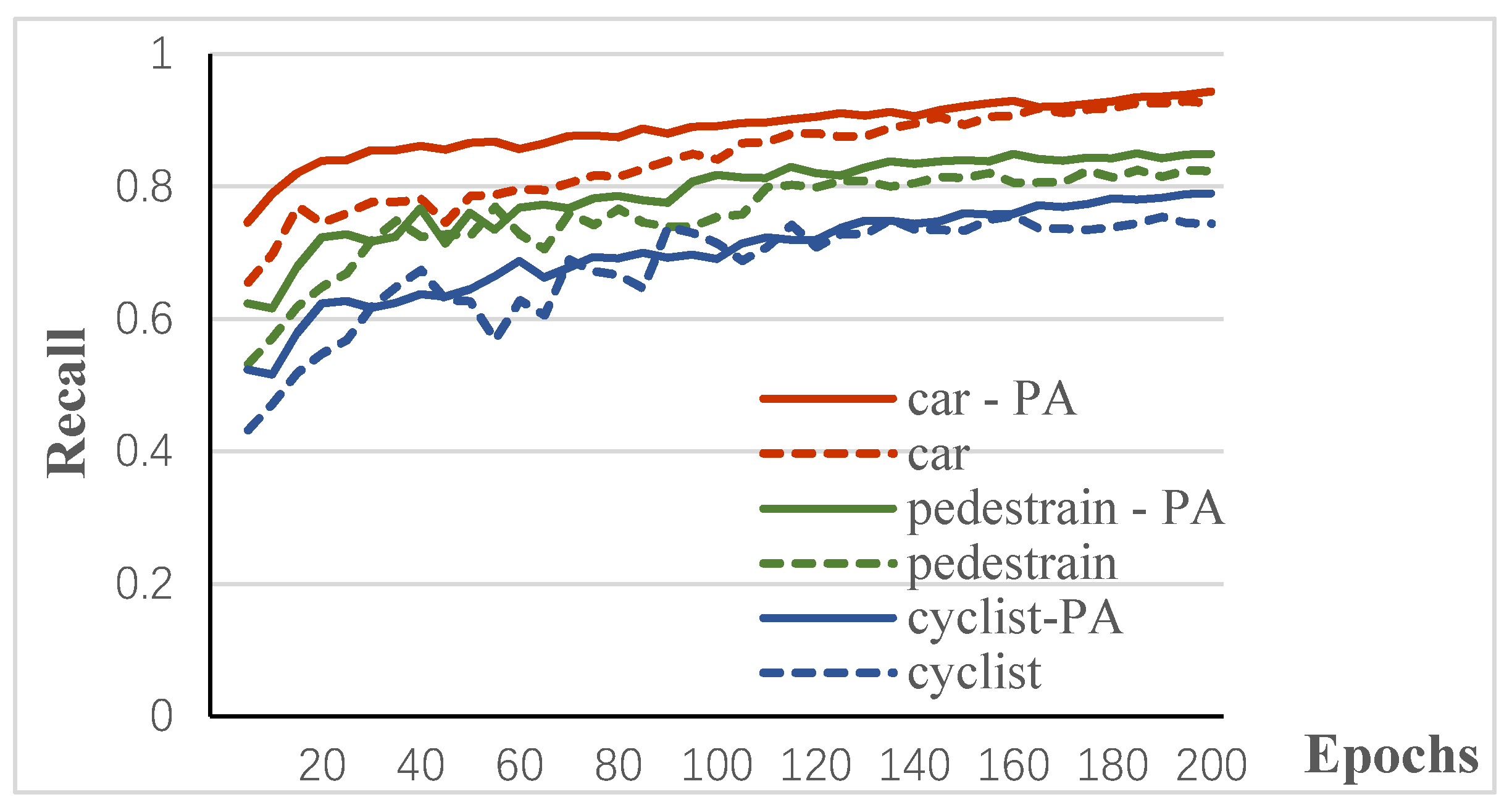
Effect of Attention Modules on 3D Proposal Recall. Our part-1 mainly aims to robustly generate coarse but high-recall 3D proposals. We compare performances of integrating different attention modules/combinations in part-1, using the final recall with 512 proposals at a 0.5 3D IoU threshold as the evaluation metric. Adding the PA module brings significant improvements, as shown in the “recall vs. epochs” curves of Figure 10. It achieves higher recall and faster convergence speed in all three classes, which benefits from the reinforcement on “representative” point-features in the full-point feature extraction process. However, we found that adding CA contributes negligibly to the performance, while using three combinations achieves the similar recalls as PA-only but the convergence speeds are slower, which can be explained as follows: although similar works as CA are widely used in fine-grained recognition of images, the difference in features between the channels is not a key factor affecting the recall.
Effect of Attention Modules on Foreground Segmentation. Our part-1 segments foreground points for estimating 3D proposals and offering candidate key-points needed by part-2. The above experiment has proved that adding point-wise attention (PA) modules to part-1 benefits to improve proposal recall. In this experiment, we evaluate our PA’s impact on the foreground point segmentation task. We compare predicted with ground-truth labels, point-wise, and evaluate precision, recall, and IoU scores, which are defined as follows:
where and respectively denote the predicted and ground-truth point sets that belong to car or pedestrian/cyclist classes. IoU score is used as the primary accuracy metric in this experiment. As shown in Table 5, we compared two variations of the part-1, one with the PA and one without. By adding PA, we increased segmentation accuracy (IoU) for all classes significantly, and both class-level recalls are improved by a large margin, which is desirable for autonomous driving, as false negatives are more likely to lead to accidents than false positives.
Effect of Attention Modules on 3D Detection Precision. In the first two rows of Table 6, we compare 3D Detection performances of KDA3D without any attention module against that of KDA3D with PA (only in part-1). As expected, the second row shows an obvious higher score, because the performance of foreground segmentation and proposal generation can greatly affect key-point densification and box refinement. In the second five rows of Table 6, we analyze the impacts of integrating different attention modules/combinations into the ROI feature extractor of part-3 on the final detection performance. The base network (the second row) is our KDA3D without any attention module in part-3. We observe that plugging CA (the fourth row) results in a nontrivial improvement over the base network, especially for pedestrian and cyclist classes, with gains of 2.88% and 2.40% on the most important “Moderate” instances. This confirms that CA designed to strengthen crucial and discriminative geometric details is beneficial for 3D bounding box refinement on small classes. The third row of Table 6 shows that adding PA only produces slightly superior results to the base network; the last three rows show that using the three combinations (PA-CA, CA-PA, CA//PA) only produces a small increase or decrease over using only CA. This phenomenon can be attributed to the fact that PA mainly aims to strengthen informative points (features), which is necessary when processing the entire input points ( = 16384) in part-1. However, most of the points in the proposal regions are target ones, selectively enhancing some points further is of little significance. In addition, in the above experiments, we found that adopting sequential arrangements (PA-CA, CA-PA) outperformed the parallel arrangement (CA//PA) and that the CA-first order performed slightly better than the PA-first order.
4.3.3. Effect of Semantic Segmentation
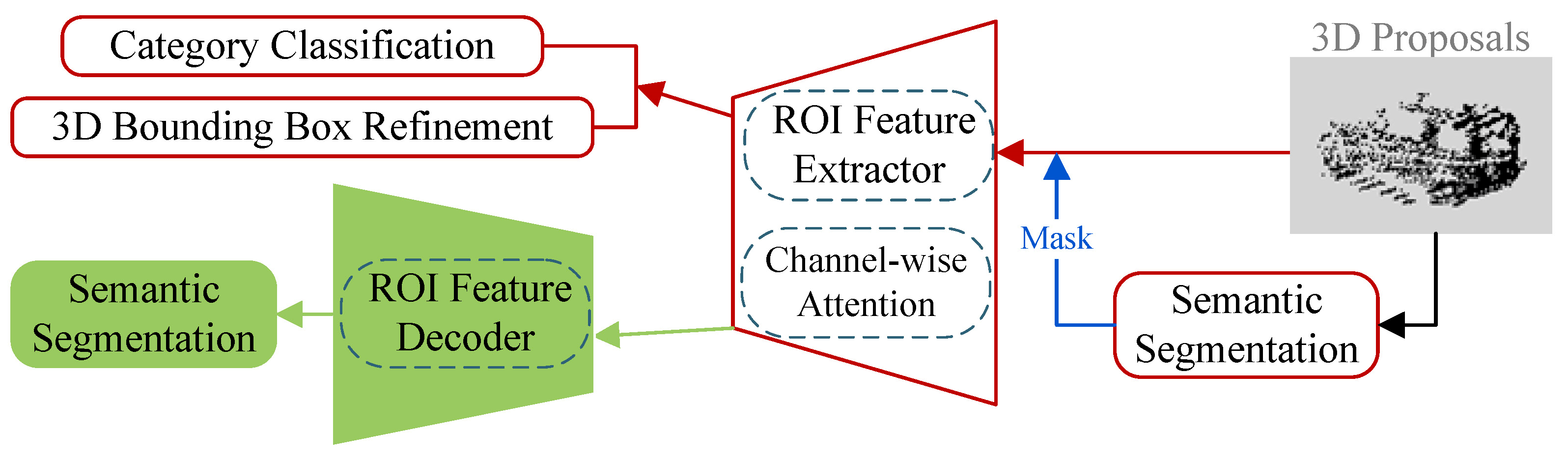
In this section, we discuss the effect of different semantic segmentation branch designs. As shown in Figure 11, the three structures to be compared are identified by different colors: “Black” uses the idea of parallel processing to indirectly associate segmentation and detection (details described in Section 3.3.1); “Blue” adds a masking modulation operation to the “Black” version, firstly uses the semantic segmentation results to recalibrate point-wise features of proposals, and then passes them to the ROI feature extractor; “Green” adds a decoding network (similar to the decoding part of the full-point feature extractor in part-1) to the ROI feature extractor and appends the semantic segmentation branch on it, which aims to create a deeper correlation between segmentation and detection.
In Table 7 (Figure 11), we take KDA3D with no semantic segmentation as the basic network, study effects of adding “Black,” “Blue,” and “Green” branches to the base network on the 3D object detection performance. As seen, the second-row “Black” version obtains better results than the first-row base version, which validates our assumption that the constraints and supervision added by semantic segmentation facilitate fine detection. We also observe that the third-row “Blue” version results in a slight decrease in AP3D compared to the “Black” one. This means that semantic segmentation results require more complex processing to accurately represent point-wise feature responses. The fourth-row “Green” version introduces additional CNNs and computational overhead but obtains the worst results, which can be attributed to the fact that too many parameters are shared by the detection and segmentation tasks in this version, resulting in an excessive emphasis on their correlation and ignoring their differences.
4.4. Qualitative Results and Discussion
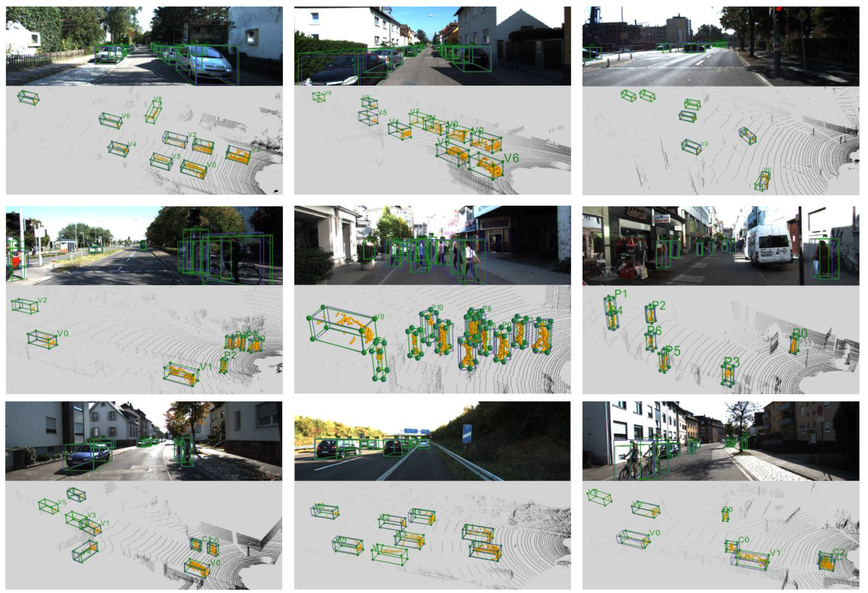
In Figure 12, we depict representative outputs of our KDA3D. For “Easy”/“Moderate” instances that are fully visible or partly occluded at a reasonable distance, our model can predict particularly accurate 3D instance segmentation masks and oriented 3D bounding boxes. For some challenging instances that are strongly overlapped or have a small number of available points, our model still performs well (e.g., dense cars in the first row and the crowd in the second row). Surprisingly, our model successfully detects many difficult and complex instances that are heavily occluded or difficult to see (e.g., V7 and V8 in first row first column; P4, P6, and P10 in second row second column; V3 and V5 in third row first column), some of which were not even labeled in the ground-truth annotations (e.g., V7 and V8 in first row second column; V3, V5, and V6 in first row third column; P0 and V3 in third row third column). Overall, these results demonstrate the excellent scalability of our KDA3D and its superior performance in 3D detection for small classes (pedestrians, cyclists) and long-range.
In fact, many state-of-the-art works may not achieve the results shown in Table 2 without the support of high-end Velodyne HDL-64E from KITTI, whereas the LIDAR sensor is arguably the most expensive additional component required for autonomous driving. Our proposed key-point densification method is designed as a separate component, which can flexibly respond to various needs and equipment. We consider that it can provide new opportunities. One could imagine a setting where moderate-end autonomous driving platforms consist of an optical camera and a moderate-price LIDAR, instead of using an expensive LIDAR with more rotating laser beams, avoiding a hefty premium while obtaining more dense and robust data. We will continue to refine and complete this vision.
In addition, we are doing board-level fusion work (not yet published) for multiple sensors, including integrating LIDAR and camera hardware, synchronizing multimodal data in time and space, and performing real-time multimodality registration. KDA3D’s key-point densification component has used these technologies to speed up the K-mean clustering, but the KDA3D runtime shown in Table 2 indicates that our acceleration work still requires further effort.
5. Conclusions
In this work, we presented KDA3D, a 3D object detector for autonomous driving scenarios. The part-1 generates 3D proposals from raw point clouds; it obtains higher recall by using the proposed point-wise attention module. The part-2 produces pseudo-point clouds from monocular images to enhance key-point densities and improve features consistency; it is optional and is mainly for multi-sensor or small/distant object detection. The part-3 performs accurate oriented 3D bounding box regression, semantic segmentation, and category classification, where the proposed channel-wise attention module and added segmentation supervision are beneficial for high-precision location. Experiments on the KITTI and nuScenes datasets show that our KDA3D outperforms state-of-the-art 3D detection methods, especially for objects with relatively less and incomplete information. In the future, we will conduct extended research in three directions: how to fully close the image/LIDAR gap, how to accelerate the inference speed of our proposed network (especially for key-point densification component), and how to better apply multi-attention for more perception tasks.
Author Contributions
Conceptualization, J.W. and M.Z.; software, J.W.; validation, J.W., B.W., and D.S.; investigation, H.W. and C.L.; data curation, H.N.; writing—original draft preparation, J.W.; writing—review and editing, J.W. and M.Z.; visualization, J.W. and B.W.; supervision, M.Z.; project administration, M.Z.; funding acquisition, M.Z.. All authors have read and agreed to the published version of the manuscript.
Funding
This research was funded by the Education Department of Jilin Province, China under grant number JJKH20200780KJ.
Conflicts of Interest
The authors declare no conflict of interest.
Appendix A. Evaluation on nuScenes Dataset
In Appendix A, we evaluate our proposed KDA3D on the newly introduced nuScenes dataset [4]. First, we briefly introduce the experimental setup. Second, we perform a comparison with state-of-the-art 3D detection methods.
Experimental Setup. The nuScenes dataset (full release in March 2019) is a more challenging 3D detection dataset that contains more than 1000 scenes in Boston and Singapore. The dataset is collected using six multi-view cameras (1600 × 900 resolution) and 32-beams LIDAR (about 40K points per frame), and 360-degree object annotations for 10 object classes are provided. The dataset consists of 28,130 training samples and 6019 validation samples, including a large number of complex traffic scenarios and challenging driving situations. Our models are trained on nuScenes train set and evaluated on nuScenes validation (val) set.
We follow the official nuScenes protocol: the evaluation results are given in terms of the average precision (AP) metric, mean Average Precision (mAP) metric, and nuScenes detection score (NDS) metric. AP is matched by thresholding the 2D center distance on the ground plane instead of IoU. NDS defined in [4] is a weighted sum between mAP, the mean average errors of location/translation (mATE), size/scale (mASE), orientation (mAOE), attribute (mAAE), and velocity (mAVE). NDS is calculated by:
here TP denotes the set of the five mean average errors. The training schedule is just the same as the schedule on the KITTI dataset. We only apply flip augmentation during training.
Comparison with State-of-the-Arts Methods. We show NDS and mAP among different methods in Table A2 and compare their APs of each class in Table A1. “Ours” refers to KDA3D and “Ours (slim)” refers to KDA3D (slim) (See Section 4.1). As illustrated in Table A2, Ours/Ours (slim) offers 2.06%/0.93% and 2.46%/0.9% performance gains in the mAP and NDS metrics compared to the second-best performing method. As shown in Table A1, not only on mAP, they also outperform other methods on AP metric, especially for classes with relatively low APs. In addition, our experiments show that the performance gain achieved by the key-point densification in nuScenes dataset is higher than that in KITTI dataset. Because the resolution of LIDAR used in nuScenes is lower than that in KITTI, this shows that our key-point densification component generating positive points (features) compensates low resolution of the LIDAR data.

Table A1.
Comparison of the 3D object detection performance of KDA3D with state-of-the-art 3D object detectors: Average Precision of 3D boxes on nuScenes’s val set.
Table A1.
Comparison of the 3D object detection performance of KDA3D with state-of-the-art 3D object detectors: Average Precision of 3D boxes on nuScenes’s val set.
| Method | Car | Ped. | Bus | Barrier | TC | Truck | Trailer | Moto | Cons. Veh | Bicycle | mAP |
|---|---|---|---|---|---|---|---|---|---|---|---|
| SECOND [6] | 75.53 | 59.86 | 29.04 | 32.21 | 22.49 | 21.88 | 12.96 | 16.89 | 0.36 | 0 | 27.12 |
| PointPillars [11] | 70.5 | 59.9 | 34.4 | 33.2 | 29.6 | 25.0 | 20.0 | 16.7 | 4.5 | 1.6 | 29.5 |
| 3D-CVF [44] | 79.69 | 71.28 | 54.96 | 47.10 | 40.82 | 37.94 | 36.29 | 37.18 | - | - | 42.17 |
| 3DSSD [17] | 81.20 | 70.17 | 61.41 | 47.94 | 31.06 | 47.15 | 30.45 | 35.96 | 12.64 | 8.63 | 42.66 |
| Ours (slim) | 81.56 | 72.03 | 62.56 | 48.65 | 40.96 | 44.35 | 33.52 | 37.23 | 6.3 | 8.76 | 43.59 |
| Ours | 82.51 | 73.21 | 63.14 | 49.05 | 41.25 | 45.32 | 35.89 | 38.92 | 7.6 | 10.35 | 44.72 |
Table A2.
Comparison of the 3D object detection performance of KDA3D with state-of-the-art 3D object detectors: mean Average Precision (mAP) and nuScenes detection score (NDS) on nuScenes’s val set.
Table A2.
Comparison of the 3D object detection performance of KDA3D with state-of-the-art 3D object detectors: mean Average Precision (mAP) and nuScenes detection score (NDS) on nuScenes’s val set.
| Method | mAP | mATE | mASE | mAOE | mAVE | AAE | NDS |
|---|---|---|---|---|---|---|---|
| SECOND [6] | 27.12 | - | - | - | - | - | - |
| PointPillars [11] | 29.5 | 0.54 | 0.29 | 0.45 | 0.29 | 0.41 | 44.9 |
| 3D-CVF [44] | 42.17 | - | - | - | - | - | 49.78 |
| 3DSSD [17] | 42.66 | 0.39 | 0.29 | 0.44 | 0.22 | 0.12 | 56.4 |
| Ours (slim) | 43.59 | 0.40 | 0.28 | 0.43 | 0.23 | 0.11 | 57.3 |
| Ours | 44.72 | 0.36 | 0.28 | 0.40 | 0.20 | 0.11 | 58.86 |
Appendix B. Details and Visualizations
In Appendix B, we provide additional technical details and more qualitative results.
Appendix B.1. Details on Network Architectures
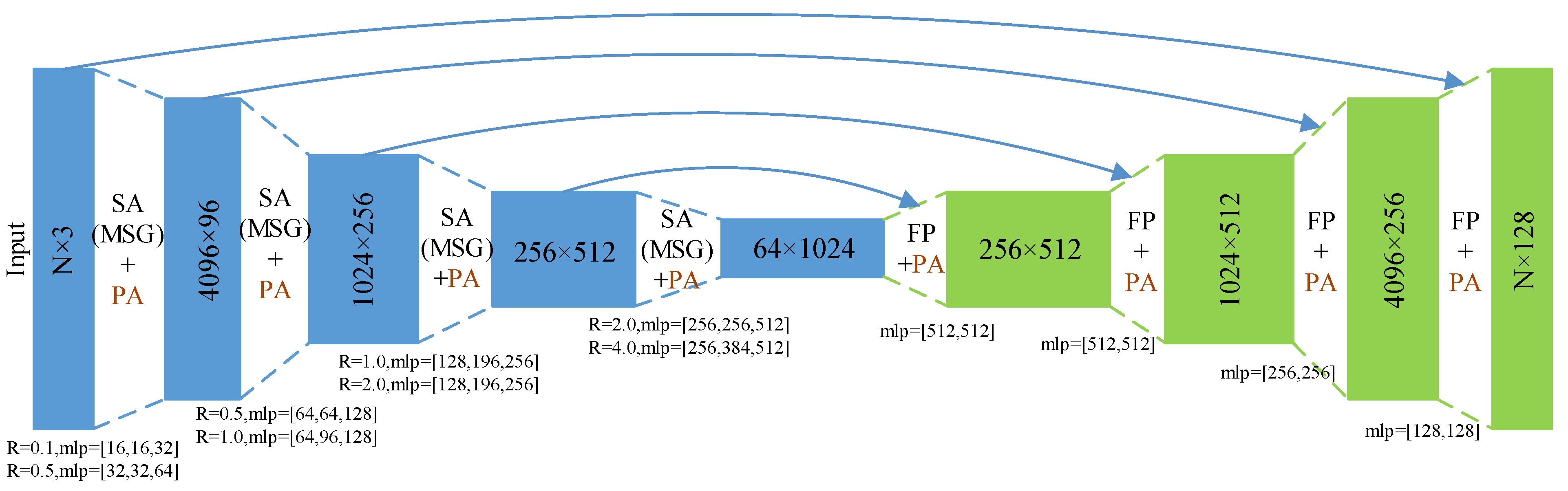
We adopt similar network architecture as in the original work of PointNet++ (with MSG) [1] for our full-point feature extractor in part-1. What is different is that we integrate the proposed point-wise attention (PA) module in each hierarchy. The detailed network architecture is shown in Figure A1. It takes a raw point cloud as input and generates global context features for each point by stacking set abstraction (SA) layers/feature propagation (FP) layers added PA modules.
Figure A1.
The detailed architecture of our full-point feature extractor based on PointNet++ (with MSG). The SA is made of Sampling layer, Grouping layer, and PointNet layer. The FP is made of Interpolation layer and Unit PointNet layer. “mlp” refers to the size of the multilayer perceptron, “R” refers to the radius/scale in the Grouping layer.

Appendix B.2. More Visualizations
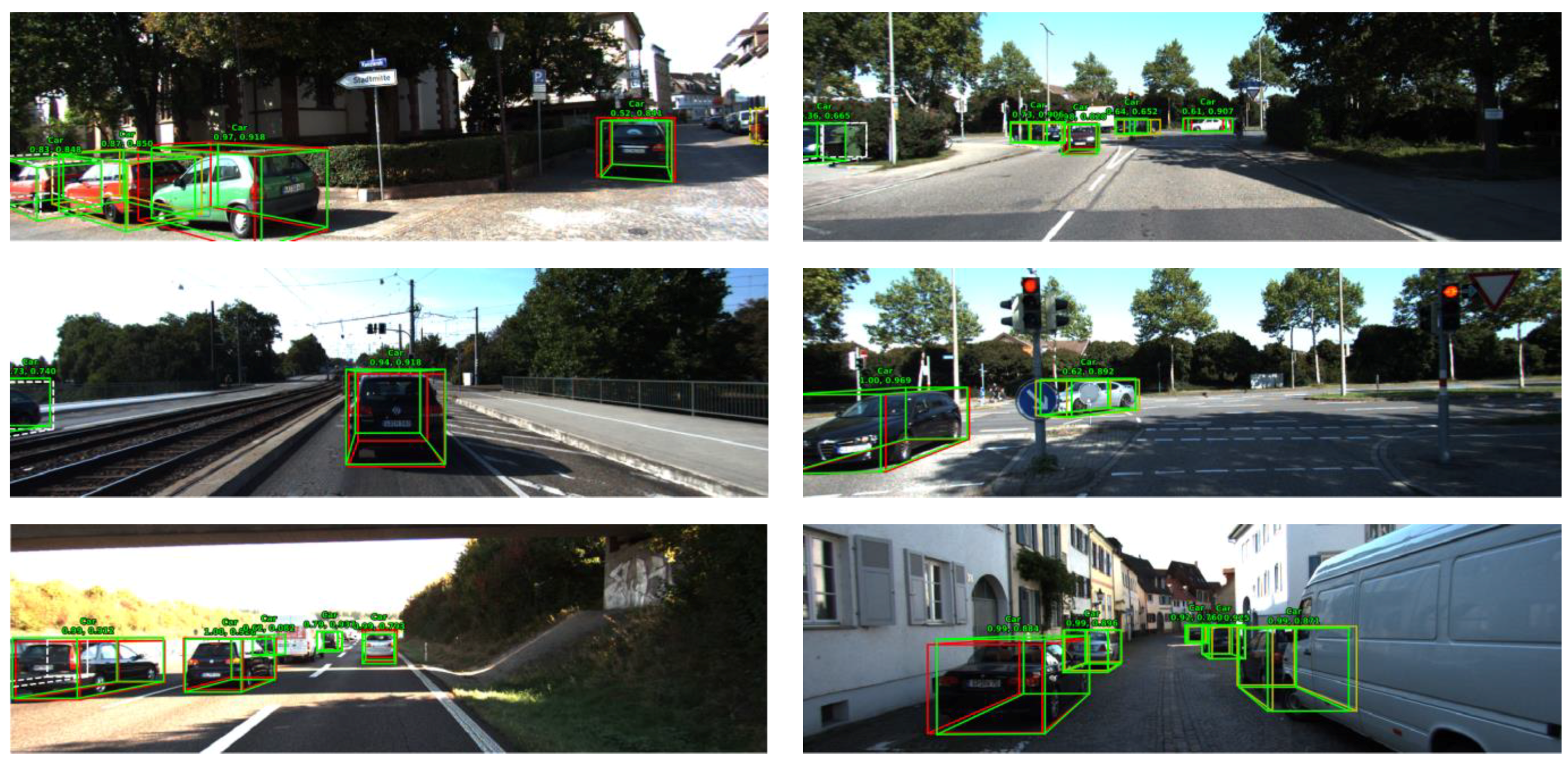
In Figure A2, we present more 3D detection results for different difficulty levels (“Easy”/“Moderate”/“Hard”) on the KITTI dataset. For better visualization, the 3D boxes detected using point clouds and images are projected onto images from the left camera, where the ground-truth boxes are shown in different colors according to their difficulty levels.
Figure A2.
Visualizations of KDA3D results on the KITTI val set. The predictions are shown with green 3D bounding boxes. The ground-truth boxes are shown in different colors according to their difficulty levels, where “Easy” instances are shown in red, “Moderate” instances are shown in yellow, and “Hard” instances are shown in white. The digits beside each box denote the confidence score (left) and the IoU (right). Best viewed in color (zoom in for details).

References
- Qi, C.R.; Yi, L.; Su, H.; Guibas, L.J. PointNet++: Deep Hierarchical Feature Learning on Point Sets in a Metric Space. In Proceedings of the Advances in Neural Information Processing Systems 30: Annual Conference on Neural Information Processing Systems 2017, Long Beach, CA, USA, 4–9 December 2017; pp. 5099–5108. [Google Scholar]
- Shi, S.; Wang, X.; Li, H. PointRCNN: 3D Object Proposal Generation and Detection from Point Cloud. In Proceedings of the 2019 IEEE/CVF Conference on Computer Vision and Pattern Recognition (CVPR); Institute of Electrical and Electronics Engineers (IEEE): Piscataway, NJ, USA, 2019; pp. 770–779. [Google Scholar]
- Geiger, A.; Lenz, P.; Urtasun, R. Are we ready for autonomous driving? The KITTI vision benchmark suite. In Proceedings of the 2012 IEEE Conference on Computer Vision and Pattern Recognition; Institute of Electrical and Electronics Engineers (IEEE): Piscataway, NJ, USA, 2012; pp. 3354–3361. [Google Scholar]
- Caesar, H.; Bankiti, V.; Lang, A.H.; Vora, S.; Liong, V.E.; Xu, Q.; Krishnan, A.; Pan, Y.; Baldan, G.; Beijbom, O. NuScenes: A multimodal dataset for autonomous driving. arXiv 2019, arXiv:1903.11027. [Google Scholar]
- Zhou, Y.; Tuzel, O. VoxelNet: End-to-End Learning for Point Cloud Based 3D Object Detection. In Proceedings of the 2018 IEEE/CVF Conference on Computer Vision and Pattern Recognition; Institute of Electrical and Electronics Engineers (IEEE): Piscataway, NJ, USA, 2018; pp. 4490–4499. [Google Scholar]
- Yan, Y.; Mao, Y.; Li, B. Second: Sparsely Embedded Convolutional Detection. Sensors 2018, 18, 3337. [Google Scholar] [CrossRef] [PubMed] [Green Version]
- Li, B.; Zhang, T.; Xia, T. Vehicle Detection from 3D Lidar Using Fully Convolutional Network. Robot. Sci. Syst. XII 2016. [Google Scholar] [CrossRef]
- Yang, B.; Luo, W.; Urtasun, R. Pixor: Real-time 3D Object Detection from Point Clouds. In Proceedings of the 2018 IEEE/CVF Conference on Computer Vision and Pattern Recognition; Institute of Electrical and Electronics Engineers (IEEE): Piscataway, NJ, USA, 2018; pp. 7652–7660. [Google Scholar]
- Simon, M.; Milz, S.; Amende, K.; Gross, H.-M. Complex-YOLO: A Euler-Region-Proposal for Real-Time 3D Object Detection on Point Clouds. Appl. Evol. Comput. 2019, 197–209. [Google Scholar] [CrossRef]
- Shi, S.; Wang, Z.; Shi, J.; Wang, X.; Li, H. From Points to Parts: 3D Object Detection from Point Cloud with Part-aware and Part-aggregation Network. IEEE Trans. Pattern Anal. Mach. Intell. 2020, 1. [Google Scholar] [CrossRef] [PubMed] [Green Version]
- Lang, A.H.; Vora, S.; Caesar, H.; Zhou, L.; Yang, J.; Beijbom, O. Pointpillars: Fast Encoders for Object Detection from Point Clouds. In Proceedings of the 2019 IEEE/CVF Conference on Computer Vision and Pattern Recognition (CVPR); Institute of Electrical and Electronics Engineers (IEEE): Piscataway, NJ, USA, 2019; pp. 12689–12697. [Google Scholar]
- Lin, T.-Y.; Goyal, P.; Girshick, R.; He, K.; Dollar, P. Focal Loss for Dense Object Detection. In Proceedings Proceedings of the IEEE International Conference on Computer Vision, Venice, Italy, 22–29 October 2017; pp. 2980–2988. [Google Scholar]
- Redmon, J.; Divvala, S.; Girshick, R.; Farhadi, A. You Only Look Once: Unified, Real-Time Object Detection. In Proceedings of the 2016 IEEE Conference on Computer Vision and Pattern Recognition (CVPR); Institute of Electrical and Electronics Engineers (IEEE): Piscataway, NJ, USA, 2016; pp. 779–788. [Google Scholar]
- Charles, R.Q.; Su, H.; Kaichun, M.; Guibas, L.J. PointNet: Deep Learning on Point Sets for 3D Classification and Segmentation. In Proceedings of the 2017 IEEE Conference on Computer Vision and Pattern Recognition (CVPR); Institute of Electrical and Electronics Engineers (IEEE): Piscataway, NJ, USA, 2017; pp. 77–85. [Google Scholar]
- Li, Y.; Bu, R.; Sun, M.; Wu, W.; Di, X.; Chen, B. Pointcnn: Convolution on x-transformed points. In Proceedings of the Advances in Neural Information Processing Systems, Montreal, QC, Canada, 3–8 December 2018; pp. 820–830. [Google Scholar]
- Yang, Z.; Sun, Y.; Liu, S.; Shen, X.; Jia, J. STD: Sparse-to-Dense 3D Object Detector for Point Cloud. In Proceedings of the 2019 IEEE/CVF International Conference on Computer Vision (ICCV); Institute of Electrical and Electronics Engineers (IEEE): Seoul, Korea, 2019; pp. 1951–1960. [Google Scholar]
- Yang, Z.; Sun, Y.; Liu, S.; Jia, J. 3DSSD: Point-based 3D Single Stage Object Detector. arXiv 2019, arXiv:2002.10187. [Google Scholar]
- Qi, C.R.; Liu, W.; Wu, C.; Su, H.; Guibas, L.J. Frustum PointNets for 3D Object Detection from RGB-D Data. In Proceedings of the 2018 IEEE/CVF Conference on Computer Vision and Pattern Recognition; Institute of Electrical and Electronics Engineers (IEEE): Piscataway, NJ, USA, 2018; pp. 918–927. [Google Scholar]
- Shin, K.; Kwon, Y.P.; Tomizuka, M. RoarNet: A Robust 3D Object Detection based on RegiOn Approximation Refinement. 2019 IEEE Intelligent Vehicles Symposium, Paris, France, 9–12 June 2019. [Google Scholar]
- Wang, Z.; Jia, K. Frustum ConvNet: Sliding Frustums to Aggregate Local Point-Wise Features for Amodal 3D Object Detection. arXiv 2019, arXiv:1903.01864, 1742–1749, 1742–1749. [Google Scholar]
- Chen, X.; Ma, H.; Wan, J.; Li, B.; Xia, T. Multi-view 3D Object Detection Network for Autonomous Driving. In Proceedings of the 2017 IEEE Conference on Computer Vision and Pattern Recognition (CVPR); Institute of Electrical and Electronics Engineers (IEEE): Piscataway, NJ, USA, 2017; pp. 6526–6534. [Google Scholar]
- Ren, S.; He, K.; Girshick, R.; Sun, J. Faster R-CNN: Towards Real-Time Object Detection with Region Proposal Networks. IEEE Trans. Pattern Anal. Mach. Intell. 2017, 39, 1137–1149. [Google Scholar] [CrossRef] [PubMed] [Green Version]
- Ku, J.; Mozifian, M.; Lee, J.; Harakeh, A.; Waslander, S.L. Joint 3D Proposal Generation and Object Detection from View Aggregation. In Proceedings of the 2018 IEEE/RSJ International Conference on Intelligent Robots and Systems (IROS); Institute of Electrical and Electronics Engineers (IEEE): Piscataway, NJ, USA, 2018; pp. 1–8. [Google Scholar]
- Simonyan, K.; Zisserman, A. Very deep convolutional networks for large-scale image recognition. arXiv 2014, arXiv:1409.1556. [Google Scholar]
- Liang, M.; Yang, B.; Wang, S.; Urtasun, R. Deep Continuous Fusion for Multi-sensor 3D Object Detection. In Proceedings of the Applications of Evolutionary Computation; Springer Science and Business Media LLC: Berlin/Heidelberg, Germany, 2018; pp. 663–678. [Google Scholar]
- Liang, M.; Yang, B.; Chen, Y.; Hu, R.; Urtasun, R. Multi-Task Multi-Sensor Fusion for 3D Object Detection. In Proceedings of the 2019 IEEE/CVF Conference on Computer Vision and Pattern Recognition (CVPR); Institute of Electrical and Electronics Engineers (IEEE): Piscataway, NJ, USA, 2019; pp. 7337–7345. [Google Scholar]
- Xie, L.; Xiang, C.; Yu, Z.; Xu, G.; Yang, Z.; Cai, D.; He, X. PI-RCNN: An Efficient Multi-sensor 3D Object Detector with Point-based Attentive Cont-conv Fusion Module. arXiv 2019, arXiv:06084. [Google Scholar]
- Lin, T.-Y.; Dollár, P.; Girshick, R.; He, K.; Hariharan, B.; Belongie, S. Feature pyramid networks for object detection. In Proceedings of the IEEE Conference on Computer Vision and Pattern Recognition, Las Vegas, Nevada, USA, 21–26 July 2016; pp. 2117–2125. [Google Scholar]
- Wei, M.; Xing, F.; You, Z. A real-time detection and positioning method for small and weak targets using a 1D morphology-based approach in 2D images. Light. Sci. Appl. 2018, 7, 18006. [Google Scholar] [CrossRef] [PubMed]
- Wang, J.; Zhu, M.; Sun, D.; Wang, B.; Gao, W.; Wei, H. MCF3D: Multi-Stage Complementary Fusion for Multi-Sensor 3D Object Detection. IEEE Access 2019, 7, 90801–90814. [Google Scholar] [CrossRef]
- Yang, Z.; Sun, Y.; Liu, S.; Shen, X.; Jia, J. IPOD: Intensive Point-based Object Detector for Point Cloud. arXiv 2018, arXiv:1812.05276. [Google Scholar]
- Jiang, M.; Wu, Y.; Lu, C. PointSIFT: A SIFT-like Network Module for 3D Point Cloud Semantic Segmentation. arXiv 2018, arXiv:00652. [Google Scholar]
- Hu, J.; Shen, L.; Sun, G. Squeeze-and-Excitation Networks. In Proceedings of the 2018 IEEE/CVF Conference on Computer Vision and Pattern Recognition; Institute of Electrical and Electronics Engineers (IEEE): Piscataway, NJ, USA, 2018; pp. 7132–7141. [Google Scholar]
- Woo, S.; Park, J.; Lee, J.-Y.; Kweon, I.S. CBAM: Convolutional Block Attention Module. In Proceedings of the Applications of Evolutionary Computation; Springer Science and Business Media LLC: Berlin/Heidelberg, Germany, 2018; pp. 3–19. [Google Scholar]
- Wang, F.; Jiang, M.; Qian, C.; Yang, S.; Li, C.; Zhang, H.; Wang, X.; Tang, X. Residual Attention Network for Image Classification. In Proceedings of the 2017 IEEE Conference on Computer Vision and Pattern Recognition (CVPR); Institute of Electrical and Electronics Engineers (IEEE): Piscataway, NJ, USA, 2017; pp. 6450–6458. [Google Scholar]
- Chen, L.; Zhang, H.; Xiao, J.; Nie, L.; Shao, J.; Liu, W.; Chua, T.-S. SCA-CNN: Spatial and Channel-Wise Attention in Convolutional Networks for Image Captioning. In Proceedings of the 2017 IEEE Conference on Computer Vision and Pattern Recognition (CVPR); Institute of Electrical and Electronics Engineers (IEEE): Piscataway, NJ, USA, 2017; pp. 6298–6306. [Google Scholar]
- Nair, V.; Hinton, G.E. Rectified linear units improve restricted boltzmann machines. In Proceedings of the 27th international conference on machine learning (ICML-10), Haifa, Israel, 21–24 June 2010; pp. 807–814. [Google Scholar]
- Krishna, K.; Murty, M.N. Genetic K-means algorithm. IEEE Trans. Syst. Man Cybern. Part B 1999, 29, 433–439. [Google Scholar] [CrossRef] [PubMed] [Green Version]
- Jain, A.K. Data clustering: 50 years beyond K-means. Pattern Recognit. Lett. 2010, 31, 651–666. [Google Scholar] [CrossRef]
- Chen, X.; Kundu, K.; Zhang, Z.; Ma, H.; Fidler, S.; Urtasun, R. Monocular 3D Object Detection for Autonomous Driving. In Proceedings of the 2016 IEEE Conference on Computer Vision and Pattern Recognition (CVPR), 20–25 June 2016; Institute of Electrical and Electronics Engineers (IEEE): Piscataway, NJ, USA; pp. 2147–2156. [Google Scholar]
- Ma, H.; Kundu, K.; Zhu, Y.; Ma, H.; Fidler, S.; Urtasun, R. 3D Object Proposals Using Stereo Imagery for Accurate Object Class Detection. IEEE Trans. Pattern Anal. Mach. Intell. 2018, 40, 1259–1272. [Google Scholar] [CrossRef] [Green Version]
- Kingma, D.P.; Ba, J.J.A. Adam: A Method for Stochastic Optimization. arXiv 2014, arXiv:1412.6980. [Google Scholar]
- Deng, J.; Dong, W.; Socher, R.; Li, L.-J.; Li, K.; Fei-Fei, L. Imagenet: A large-scale hierarchical image database. In Proceedings of the 2009 IEEE Conference on Computer Vision and Pattern Recognition, Miami, FL, USA, 20–25 June 2009; pp. 248–255. [Google Scholar]
- Yoo, J.H.; Kim, Y.; Kim, J.S.; Choi, J.W. 3D-CVF: Generating Joint Camera and LiDAR Features Using Cross-View Spatial Feature Fusion for 3D Object Detection. arXiv 2004, arXiv:12636. [Google Scholar]
Figure 1.
The architecture of the proposed KDA3D: part-1 for 3D foreground segmentation and proposal generation; part-2 (optional) for point cloud density enhancement; part-3 for semantic segmentation, 3D box refinement, and category classification.
Figure 1.
The architecture of the proposed KDA3D: part-1 for 3D foreground segmentation and proposal generation; part-2 (optional) for point cloud density enhancement; part-3 for semantic segmentation, 3D box refinement, and category classification.

Figure 2.
Architecture of our full-point feature extractor with the proposed point-wise attention (PA) modules.
Figure 2.
Architecture of our full-point feature extractor with the proposed point-wise attention (PA) modules.

Figure 3.
Illustration of the key-point densification process. Steps (1)–(2): we select the “key-points” from raw point clouds based on foreground scores and their distances, and project them onto the camera image plane to get key-pixels (in pink); Step (3): we perform K-means clustering in key-pixels’ neighborhoods to search the extension-pixels that are “close” to key-pixels; Step (4): we roughly estimate depths of extension-pixels, and back-project them to 3D space to generate the target pseudo-point clouds; finally, we optimize “pseudo + raw” points (features) to construct the compact enhanced ones.

Figure 4.
Illustration of target region generation and K-means clustering process (region size d is 5 and the number of clusters is 16).
Figure 4.
Illustration of target region generation and K-means clustering process (region size d is 5 and the number of clusters is 16).

Figure 5.
Illustration of the pseudo-point cloud generation process with depth estimation of extension-pixels.
Figure 5.
Illustration of the pseudo-point cloud generation process with depth estimation of extension-pixels.

Figure 6.
The pseudocode of the proposed sorting simplification strategy.

Figure 7.
Architecture of our region of interest (ROI) feature extractor with the proposed channel-wise attention (CA) modules.
Figure 7.
Architecture of our region of interest (ROI) feature extractor with the proposed channel-wise attention (CA) modules.

Figure 8.
Precision-recall curves of our methods for 3D object detection on the most important “Moderate” instances of the KITTI val set. The solid lines refer to KDA3D and the dotted lines refer to KDA3D (slim).
Figure 8.
Precision-recall curves of our methods for 3D object detection on the most important “Moderate” instances of the KITTI val set. The solid lines refer to KDA3D and the dotted lines refer to KDA3D (slim).

Figure 9.
Visualizations of the results of key-point densification. (a) is a representative view of raw point clouds. (b) is the view of key-points selected according to our distance preference strategy. (c) is the view of “key + pseudo” points (pseudo-points are generated by K-means from the corresponding image). (d) is the view of compact ”raw + pseudo” points reorganized according to our sorting simplification strategy.

Figure 10.
Recall curves of embedding attention modules in part-1 for the three classes. The solid lines refer to embedding PA, and the dotted lines refer to no-attention.
Figure 10.
Recall curves of embedding attention modules in part-1 for the three classes. The solid lines refer to embedding PA, and the dotted lines refer to no-attention.

Figure 11.
Comparison of three semantic segmentation branch designs. The three designs are shown in black, blue and green.
Figure 11.
Comparison of three semantic segmentation branch designs. The three designs are shown in black, blue and green.

Figure 12.
Qualitative results of KDA3D on the KITTI val set. For each sample, the upper part is the image and the lower part is a representative view of the corresponding point clouds. The ground-truth boxes are shown in purple, while the detected objects are shown with green 3D bounding boxes. 3D instance segmentation masks on point clouds are shown in yellow. Digit and letter beside each box denote instance ID and the class, with “V” for car, “P” for pedestrian, and “C” for cyclist. The orientation (driving direction) of each box is specified by the position of the digit and letter. Best viewed in color (zoom in for details). See Section 4.4 for more discussion on the results.

Table 1.
Intersection over union (IoU) threshold settings for box refinement and classification.
| Dataset | Class | 3D IoU Threshold | Classification | Box Regression |
|---|---|---|---|---|
| KITTI dataset | Car | Negative IoU threshold | [0.05, 0.45] | [0, 0.55) |
| Positive IoU threshold | [0.6, 1] | [0.55, 1] | ||
| Pedestrian & Cyclist | Negative IoU threshold | [0, 0.35] | [0, 0.45) | |
| Positive IoU threshold | [0.5, 1] | [0.45, 1] |
Table 2.
Comparison of the 3D object detection and location performance of KDA3D with state-of-the-art 3D object detectors: Average Precision (AP3D in %) of 3D boxes and Average Precision (APBEV in %) of bird’s eye view boxes on KITTI’s val set. We use a 3D IoU threshold of 0.7 for the car class, and 0.5 for the pedestrian and cyclist classes.
| Class | Method | Type | Runtime (s) | 3D Location | |||||
|---|---|---|---|---|---|---|---|---|---|
| Easy | Mode | Hard | Easy | Mode | Hard | ||||
| Car | AVOD-FPN [23] | Fusion | 0.1 | 84.41 | 74.44 | 68.65 | - | - | - |
| MV3D [21] | Fusion | 0.36 | 71.29 | 62.68 | 56.56 | 86.55 | 78.10 | 76.67 | |
| F-PointNet [18] | Fusion | 0.17 | 83.76 | 70.92 | 63.65 | 88.16 | 84.02 | 76.44 | |
| ContFusion [25] | Fusion | 0.06 | 86.32 | 73.25 | 67.81 | 95.44 | 87.34 | 82.43 | |
| VoxelNet [5] | LIDAR | 0.23 | 81.97 | 65.46 | 62.85 | 89.60 | 84.81 | 78.57 | |
| SECOND [6] | LIDAR | 0.05 | 87.43 | 76.48 | 69.10 | 89.96 | 87.07 | 79.66 | |
| PointRCNN [2] | LIDAR | 0.1 | 88.88 | 78.63 | 77.38 | - | - | - | |
| Ours (slim) | LIDAR | 0.1 | 87.66 | 77.68 | 77.45 | 89.98 | 87.45 | 85.45 | |
| Ours | Fusion | 0.13 | 88.45 | 78.85 | 78.46 | 90.18 | 87.69 | 86.93 | |
| AVOD-FPN [23] | Fusion | 0.1 | - | 58.8 | - | - | - | - | |
| F-PointNet [18] | Fusion | 0.17 | 70.00 | 61.32 | 53.59 | 72.38 | 66.39 | 59.57 | |
| Ped. | VoxelNet [5] | LIDAR | 0.23 | 57.86 | 53.42 | 48.87 | 65.95 | 61.05 | 56.98 |
| Ours (slim) | LIDAR | 0.1 | 58.12 | 55.86 | 50.36 | 64.21 | 59.63 | 54.36 | |
| Ours | Fusion | 0.12 | 63.34 | 60.12 | 54.36 | 70.21 | 67.34 | 61.24 | |
| AVOD-FPN [23] | Fusion | 0.1 | - | 49.7 | - | - | - | - | |
| F-PointNet [18] | Fusion | 0.17 | 77.15 | 56.49 | 53.37 | 81.82 | 60.03 | 56.32 | |
| Cyc. | VoxelNet [5] | LIDAR | 0.23 | 67.17 | 47.65 | 45.11 | 74.41 | 52.18 | 50.49 |
| Ours (slim) | LIDAR | 0.1 | 73.81 | 55.60 | 52.19 | 75.84 | 59.28 | 55.69 | |
| Ours | Fusion | 0.12 | 77.19 | 57.43 | 54.56 | 79.39 | 60.31 | 57.14 | |
Table 3.
3D object detection performances of the detectors using different key-point densification strategies: Average Precision (AP3D in %) of 3D boxes on KITTI’s val set. We use a 3D IoU threshold of 0.7 for the car class and 0.5 for the pedestrian and cyclist classes. The base detector is the KDA3D (slim). The strategy in the last row is KDA3D’s final choice.
| Key-point Densification Strategies | Car | Pedestrian | Cyclist | ||||||||
|---|---|---|---|---|---|---|---|---|---|---|---|
| Easy | Mode | Hard | Easy | Mode | Hard | Easy | Mode | Hard | |||
| Base: KDA3D (slim) | 87.66 | 77.68 | 77.45 | 58.12 | 55.86 | 50.36 | 73.81 | 55.60 | 52.19 | ||
| Base + full-points | 87.86 | 76.98 | 78.21 | 59.13 | 55.97 | 52.14 | 74.56 | 56.96 | 52.65 | ||
| Base +key-points | foreground scores (>0.3,0.2,0.2) | 88.59 | 78.69 | 77.96 | 61.23 | 58.93 | 52.68 | 75.26 | 57.25 | 53.01 | |
| distance preference strategy | add | 88.41 | 77.96 | 78.54 | 62.69 | 60.46 | 54.11 | 78.12 | 57.32 | 54.47 | |
| cut | 87.68 | 77.93 | 77.58 | 60.32 | 58.46 | 52.34 | 75.46 | 57.21 | 52.11 | ||
| compact | 88.45 | 78.85 | 78.46 | 63.34 | 60.12 | 54.36 | 77.19 | 57.43 | 54.56 | ||
Table 4.
Comparison of different K-means clustering settings: Average Precision (AP3D in %) of 3D boxes on KITTI’s val set at "Moderate" difficulty. We use a 3D IoU threshold of 0.7 for the car class and 0.5 for the pedestrian and cyclist classes. The setting in the third row is KDA3D’s final choice.
| K-means Clustering | Runtime(s) | Car | Pedestrian | Cyclist | |
|---|---|---|---|---|---|
| Iterations = 20 | Clusters = 4 | 0.14/0.13/0.13 | 78.69 | 60.11 | 58.13 |
| Clusters = 8 | 0.14/0.12/0.12 | 78.83 | 59.31 | 57.45 | |
| Clusters = 16 | 0.13/0.12/0.12 | 78.85 | 60.12 | 57.43 | |
| Iterations = 40 | Clusters = 16 | 0.14/0.13/0.12 | 78.74 | 59.86 | 59.01 |
Table 5.
KDA3D’s foreground point segmentation performance. IoU is used as the primary accuracy metric. All the values in this table are in percentages. The method in the second/fourth row is KDA3D’s final choice.
Table 5.
KDA3D’s foreground point segmentation performance. IoU is used as the primary accuracy metric. All the values in this table are in percentages. The method in the second/fourth row is KDA3D’s final choice.
| Class-level | Part-1 of KDA3D | Foreground Point Segmentation | ||
|---|---|---|---|---|
| Precision | Recall | IoU | ||
| Car | without PA | 69.5 | 94.6 | 65.1 |
| with PA | 70.1 | 96.4 | 66.8 | |
| Pedestrian & Cyclist | without PA | 47.3 | 51.2 | 42.1 |
| with PA | 48.6 | 55.6 | 44.3 | |
Table 6.
3D object detection performances of detectors embedding different attention modules/ combinations in part-1 and part-3: Average Precision (AP3D in %) of 3D boxes on KITTI’s val set. We use a 3D IoU threshold of 0.7 for the car class and 0.5 for the pedestrian and cyclist classes. The method in the fourth row is KDA3D’s final choice.
| Part-1 | Part-3 | Car | Pedestrian | Cyclist | ||||||||||
| PA | PA | CA | PA//CA | CA-PA | PA-CA | Easy | Mode | Hard | Easy | Mode | Hard | Easy | Mode | Hard |
| 87.35 | 76.86 | 75.93 | 60.24 | 55.97 | 50.42 | 73.36 | 55.74 | 51.12 | ||||||
| √ | 87.86 | 77.34 | 76.65 | 62.81 | 57.24 | 52.12 | 75.94 | 55.03 | 52.14 | |||||
| √ | √ | 87.74 | 78.13 | 76.12 | 63.14 | 57.42 | 53.24 | 76.36 | 55.74 | 52.68 | ||||
| √ | √ | 88.45 | 78.85 | 78.46 | 63.34 | 60.12 | 54.36 | 77.19 | 57.43 | 54.56 | ||||
| √ | √ | 88.12 | 78.45 | 77.69 | 63.35 | 58.96 | 54.01 | 77.20 | 56.98 | 53.75 | ||||
| √ | √ | 88.67 | 78.74 | 78.51 | 63.45 | 59.89 | 54.21 | 77.34 | 57.12 | 54.15 | ||||
| √ | √ | 88.37 | 78.61 | 78.31 | 63.40 | 59.77 | 54.14 | 77.53 | 57.06 | 53.96 | ||||
Table 7.
3D object detection performances of detectors adopting different semantic segmentation branch designs. Average Precision (AP3D in %) of 3D boxes on KITTI’s val set. We use a 3D IoU threshold of 0.7 for the car class and 0.5 for the pedestrian and cyclist classes. The baseline detector is our KDA3D without any semantic segmentation branch. The design in the second row is KDA3D’s final choice.
| Semantic Segmentation | Car | Pedestrian | Cyclist | ||||||
|---|---|---|---|---|---|---|---|---|---|
| Easy | Mode | Hard | Easy | Mode | Hard | Easy | Mode | Hard | |
| Base: KDA3D without semantic segmentation | 88.57 | 77.95 | 77.01 | 62.31 | 59.65 | 52.11 | 77.59 | 57.21 | 52.78 |
| Base + ROI segmentation head (in black) | 88.45 | 78.85 | 78.46 | 63.34 | 60.12 | 54.36 | 77.19 | 57.43 | 54.56 |
| Base + ROI segmentation mask (in blue) | 88.38 | 78.21 | 78.32 | 64.21 | 59.75 | 54.21 | 77.21 | 56.79 | 54.76 |
| Base + ROI feature decoder + segmentation head (in green) | 86.78 | 76.87 | 76.58 | 63.11 | 59.96 | 53.21 | 75.45 | 56.87 | 53.22 |
© 2020 by the authors. Licensee MDPI, Basel, Switzerland. This article is an open access article distributed under the terms and conditions of the Creative Commons Attribution (CC BY) license (http://creativecommons.org/licenses/by/4.0/).
Share and Cite
MDPI and ACS Style
Wang, J.; Zhu, M.; Wang, B.; Sun, D.; Wei, H.; Liu, C.; Nie, H. KDA3D: Key-Point Densification and Multi-Attention Guidance for 3D Object Detection. Remote Sens. 2020, 12, 1895. https://0-doi-org.brum.beds.ac.uk/10.3390/rs12111895
AMA Style
Wang J, Zhu M, Wang B, Sun D, Wei H, Liu C, Nie H. KDA3D: Key-Point Densification and Multi-Attention Guidance for 3D Object Detection. Remote Sensing. 2020; 12(11):1895. https://0-doi-org.brum.beds.ac.uk/10.3390/rs12111895
Chicago/Turabian StyleWang, Jiarong, Ming Zhu, Bo Wang, Deyao Sun, Hua Wei, Changji Liu, and Haitao Nie. 2020. "KDA3D: Key-Point Densification and Multi-Attention Guidance for 3D Object Detection" Remote Sensing 12, no. 11: 1895. https://0-doi-org.brum.beds.ac.uk/10.3390/rs12111895
Note that from the first issue of 2016, this journal uses article numbers instead of page numbers. See further details here.