Predicting Soybean Yield at the Regional Scale Using Remote Sensing and Climatic Data

Abstract

Crop yield modeling at the regional level is one of the most important methods to ensure the profitability of the agro-industrial economy and the solving of the food security problem. Due to a lack of information about crop distribution over large agricultural areas, as well as the crop separation problem (based on remote sensing data) caused by the similarity of phenological cycles, a question arises regarding the relevance of using data obtained from the arable land mask of the region to predict the yield of individual crops. This study aimed to develop a regression model for soybean crop yield monitoring in municipalities and was conducted in the Khabarovsk Territory, located in the Russian Far East. Moderate Resolution Imaging Spectroradiometer (MODIS) data, an arable land mask, the meteorological characteristics obtained using the VEGA-Science web service, and crop yield data for 2010–2019 were used. The structure of crop distribution in the Khabarovsk District was reproduced in experimental fields, and Normalized Difference Vegetation Index (NDVI) seasonal variation approximating functions were constructed (both for total district sown area and different crops). It was found that the approximating function graph for the experimental fields corresponds to a similar graph for arable land. The maximum NDVI forecast error on the 30th week in 2019 using the approximation parameters according to 2014–2018 did not exceed 0.5%. The root-mean-square error (RMSE) was 0.054. The maximum value of the NDVI, as well as the indicators characterizing the temperature regime, soil moisture, and photosynthetically active radiation in the region during the period from the 1st to the 30th calendar weeks of the year, were previously considered as parameters of the regression model for predicting soybean yield. As a result of the experiments, the NDVI and the duration of the growing season were included in the regression model as independent variables. According to 2010–2018, the mean absolute percentage error (MAPE) of the regression model was 6.2%, and the soybean yield prediction absolute percentage error (APE) for 2019 was 6.3%, while RMSE was 0.13 t/ha. This approach was evaluated with a leave-one-year-out cross-validation procedure. When the calculated maximum NDVI value was used in the regression equation for early forecasting, MAPE in the 28th–30th weeks was less than 10%.

1. Introduction

Soybean is one of the main crops in the global agro-industrial complex [1]. Worldwide, soybean production ranks fourth among all grain and leguminous crops (after rice, wheat, and corn) (http://fao.org/faostat), while the gross yield of the crop has increased by more than 50% in the 10 years from 2008 to 2018—that is, from 220 million to 340 million tons (http://www.indexbox.ru). In the Russian Far East, soybean is the main cultivated crop; in 2018, the share of the four southern Far Eastern regions that have a common border with China accounted for more than 50% of the total soybean sowing area in Russia (https://www.gks.ru). That is why soybean is one of the main crops that allows to formulate a food security strategy at the government level in different countries, which is an urgent task in conditions of economic crisis [2] and, in particular, the expected consequences of COVID-19 [3]. Thus, in order to fulfill a number of tasks, for example, in planning sown areas and making decisions related to the product’s sale, it is necessary to pre-evaluate yield at the regional level.

The assessment of soybean yield at the field level was carried out in Reference [4,5]. These studies show that vegetation indexes (i.e., the Normalized Difference Vegetation Index (NDVI) and the Triangular Vegetation Index (TVI)) are related to cover crop biomass and, hence, yield [5]. However, widely used yield analysis methods applied to individual fields, taking into account soil and agrochemical characteristics, along with remote sensing indicators, are not always applicable at the regional level [6].

Remote sensing data are often extracted using arable land masks in crop yield modeling at the territory level. The applicability of this method for a specific region requires additional study, which is associated with a different degree of signal influence from different cultures on the final result. The influence of arable land structure on the values of vegetative indices was estimated in Reference [7,8]. For example, in the Canadian prairies, where most annual crops have similar phenological cycles, it is easy enough to define the plot of the seasonal vegetation indices’ variation, and, accordingly, to set aside arable land and use it in crop modeling [9]. In other cases, due to the different phenological cycles of annual and perennial grasses and winter and spring crops, applying an arable land mask to assess the yield of a particular crop is not a priori possible. These results are very interesting from a practical point of view; they highlight the possibility of using remote sensing data obtained for arable land masks in the Russian Far East, similar in climatic conditions to some provinces of Canada. In the Russian Far East regions, due to cold winters, winter crops are practically not cultivated and it can be expected that the main crops have similar phenological cycles. In Reference [10], the authors used a static mask throughout the European Union (EU) to study the correlation of remote sensing data with official crop statistics. An empirical model for predicting crop yields in areas with crop diversity is presented in Reference [11]. Remote sensing data obtained from a common arable land mask were used to calculate wheat yield in Europe (in which the wheat share in the total sown area of different regions was used as a correction factor). Researchers from the USA [12] compared the effectiveness of using a single crop mask with a common arable land mask as part of a study to predict corn and soybean yields. As a result, inclusion of information related to crop phenology significantly improved model performance. In Reference [13], the researchers estimated the relationship between major USA crops’ yield and different time series of Moderate Resolution Imaging Spectroradiometer (MODIS) products for specific crops, including NDVI. In particular, it was shown that the yields from nine crops (i.e., barley, canola, corn, cotton, potatoes, sorghum, soybeans, sugar beets, and wheat) exhibited positive correlations with all vegetation indexes.

Recently, along with traditional trend methods and year-analog methods, regression models with climatic indicators and Earth remote sensing data as independent variables have been used to predict crop yield at the district or regional level [14,15]. The main indicators reflecting the state of arable land at certain times are the values of vegetation indices calculated from satellite images [16,17,18]. At the same time, a set of meteorological factors that include both individual indicators (temperature, humidity, etc.) and integrated climate characteristics can determine a municipality’s production conditions and crop yields [19]. For example, Balaghi et al. [20] found a strong relation between rainfall in vegetation periods and wheat yield in most provinces of Morocco, and Maas et al. [21] used photosynthetically active radiation (PAR) to predict crop yield.

Differences in the climatic conditions of neighboring municipalities are especially characteristic of the regions and subsequent districts in the Russian Far East due to their significant area. The agriculture in these regions is influenced by the complex relief and the specifics of a monsoon climate, which, first of all, is manifested for the Primorskiy and Khabarovsk territories [22,23].

Crop yield modeling studies at the regional level using remote sensing data in Russia have suggested the use of maximum NDVI values as one of the predictors of the regression model. In Reference [24], it was indicated that the maximum NDVI calculated from the mask of the determined culture is the most stable indicator among all possible NDVI composites, and is also the most suitable for predicting spring crops. Bereza et al. [25] used the term early forecasting for winter crops—in particular, wheat—and described yield forecasting at the regional level using NDVI from mid-May to mid-June when plants are heading and flowering begins. However, this NDVI value is actually the first maximum of early cultures; the second maximum characteristic of later cultures (for the Belgorod region) is observed at the end of July [26]. Thus, the considered approach can also be called yield prediction using the maximum NDVI. In general, the use of such methods is characteristic of the western regions of Russia. At the same time, in the Russian Far East, which is the main producer of soybeans in Russia, there are no structured ground-based observation data that make it possible to accurately identify soybean masks for most municipalities in the retrospective period and to compare them with remote sensing data. According to previous studies for various municipalities in the south of the Far East, it was found that the maximum NDVI values for soybeans correspond to mid-July to early August (28th–32nd calendar weeks) [27]. These calendar dates correspond to the R4–R6 stages (i.e., full pod, beginning seed, and full seed) for soybeans in the south of the Russian Far East [28].

The main objective of this article was to assess the relationships between soybean yield and the NDVI maximum and meteorological variables at the regional scale in the Khabarovsk District. Obtaining actual NDVI maximum values using weekly composites reduces the effectiveness of early forecasting, which is associated with the expectation of the next composite following the maximum value, as well as time-consuming data processing. Thus, it is proposed to apply the method of approximating NDVI seasonal variation using Gaussian function parameters for previous years for the prediction of the maximum value. This approach makes it possible to determine the maximum NDVI at an earlier stage and to further use this indicator in the regression model to predict soybean yield in the study area. The results obtained in different studies do not deny the possibility of using NDVI values of different periods of the vegetation cycle as one of the predictors of the regression model [29]. However, NDVI maxima are mainly used to ensure the highest accuracy of crop yield prediction.

Thus, at the first stage of the study, we investigated the dynamics of the seasonal NDVI variation for the main crops of the district based on experimental fields to establish the proportions of growing crops in the Khabarovsk District arable land area. As mentioned above, the use of arable land masks to predict individual crops is justified only if the main crops have similar phenological cycles. Although winter crops do not grow in the territory of the Khabarovsk region, it seems quite logical to assess the NDVI dynamics for the main crops grown in experimental fields, as well as to construct a model of arable land (taking into account the ratio of main crops). Using the same approach to calculate the NDVI index in the model and for the arable land of the entire municipal region provides the possibility of using remote sensing data on the arable land mask to predict soybean yield (as soybean is the main crop of this region).

2. Materials and Methods

2.1. Study Area

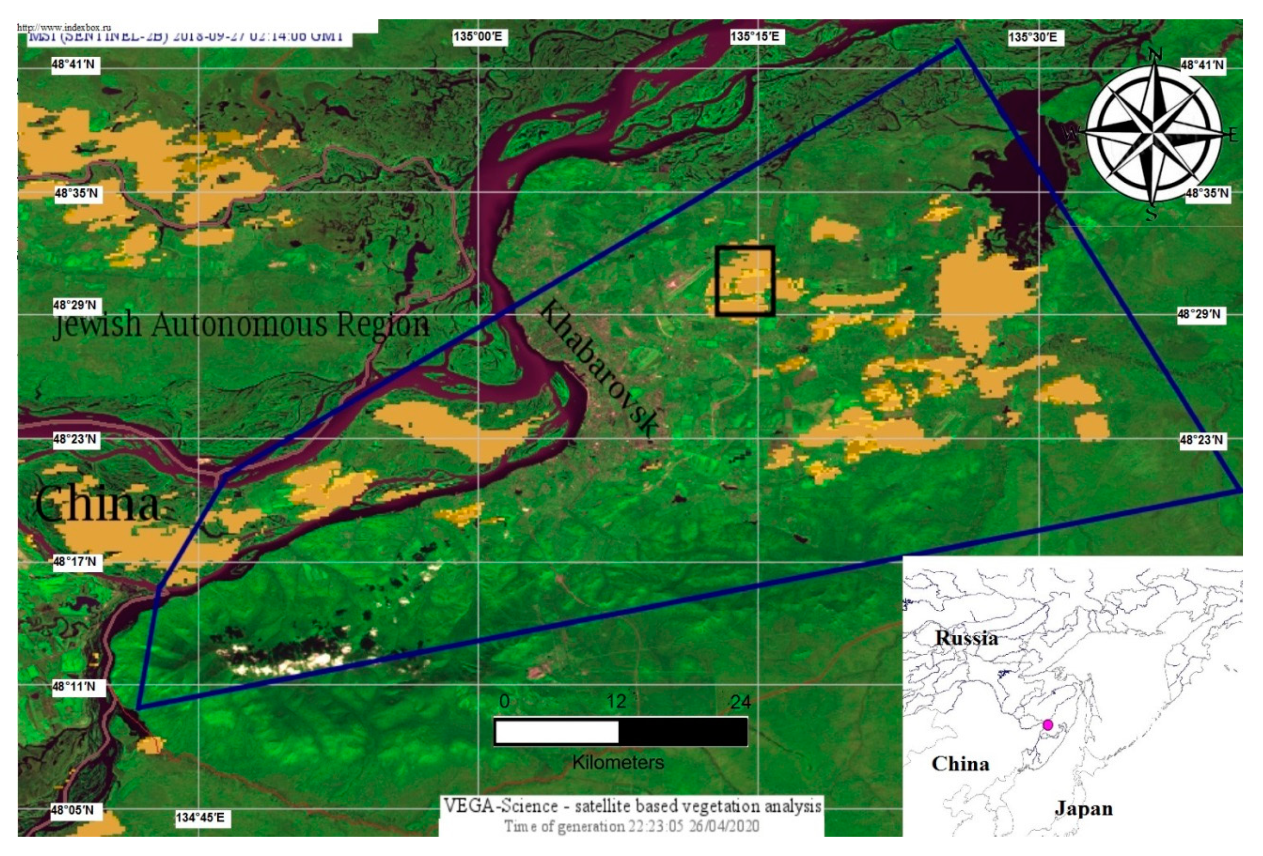
2.1.1. Khabarovsk District Area

The study area was located in the southern part of Khabarovsk Municipal District at 48°10′–48°41′N and 134°45′–135°35′E in the Middle Amur Region (Figure 1). The natural borders of the area are the Amur River basin in the north and the Big and Small Khekhtsir ranges in the south (the total area is about 6000 km²). The region displays monsoon features and is characterized by moderately cold winters with little snow, and warm, excessively moist summers. The alluvial and meadow alluvial soils of the Amur River valley (i.e., Khabarovsk suburbs and the Russian part of Big Ussuriyskiy island) are very suitable for agriculture [30]. Plenty of moisture, sunlight, and good soil conditions allow cultivating soybean [31]. The Khabarovsk District is the leading agricultural municipality of the Khabarovsk Territory. The total arable land in the Khabarovsk region in 2018 amounted to more than 28,000 ha or almost 35% of the arable land throughout the Khabarovsk Territory.

Table 1. The sown areas’ structure by crops (Khabarovsk district, 2018).

Crop	Soybean	Wheat	Oat	Potato	Forage Grasses	The Rest of the Crops	Total
Sown area, ha	16,976	1382	1748	1692	4568	1833	28,200
Percentage	60.2	4.9	6.2	6.0	16.2	6.5	100

shows that more than 60% of the arable land in the study area (about 17,000 hectares) is occupied by soybean planting, while the crops are mainly represented by spring wheat (4.9%) and oat (6.2%). Soybean is sown on 1st decade (10-day period) of May and harvested on 3rd decade of September. Growth duration of soybean is 135 days. Oat and spring wheat are sown on 2nd decade of May and harvested on 3rd decade of August. Growth duration of these crops is 95 days. The share of annual and perennial forage grasses exceeds 16%, with about a further 6% given for potato growing and the remaining 6.5% for other crops.

2.1.2. Experimental Sites

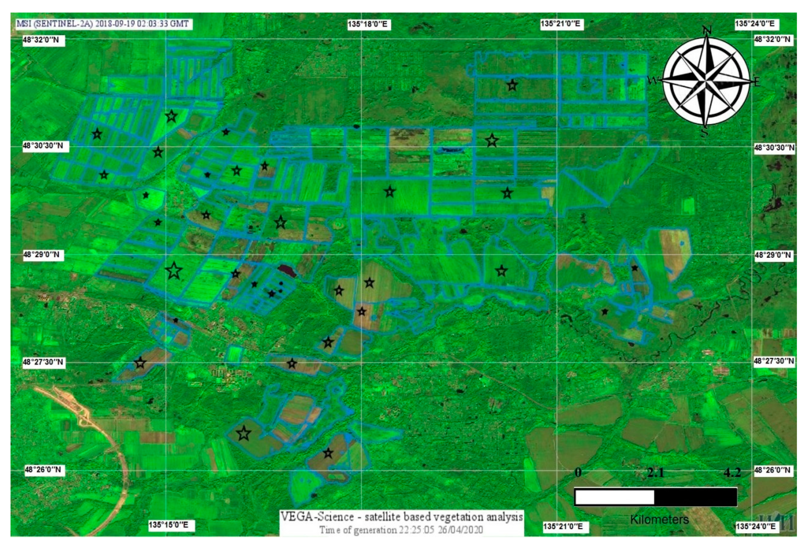
The experimental fields of the Far East Research Institute of Agriculture are located in the northern part of the study area (to the north-east of Khabarovsk) between the villages of Mirnoe and Sergeevka (Khabarovsk Municipal District). This arable land has brown-podzol and brown-meadow soil compositions. Figure 2 shows the fields of the Institute (where the researched fields are marked with stars). Twenty-one experimental soybean fields (total area is 670 ha), 14 fields of oats (360 ha), 7 fields of wheat (160 ha), and 15 fields with natural forage grasses (410 ha) were studied from 2014 to 2018. The minimum area of an individual field was 7.3 ha, and the maximum was 136 ha.

2.2. Data Acquisition and Processing

Field average NDVI calculations were performed using weekly field composite values (formed to CSV file) from the VEGA-Science web service (http://sci-vega.ru/). These composite values were a result of image processing. Images were based on remote measurements of the arable land’s spectral reflectance characteristics [32,33] and were obtained using the MODIS of the Terra satellite, which uses the atmospheric correction procedure in spectral channels in the ranges of 0.629–0.670 μm (RED) and 0.841–0.876 μm (NIR) with a spatial resolution of 250 m (standard data product MOD09 V006) [34].

The NDVI was calculated as follows:

$$NDVI=\frac{NIR-RED}{NIR+RED},$$

(1)

where RED and NIR stand for the spectral reflectance measurements acquired in the red (visible) and the near-infrared regions, respectively.

The climatic characteristics of the Khabarovsk District, including precipitation, soil temperature, humidity, and photosynthetically active radiation (PAR), were reanalyzed data that combined ground-based and remote observation data averaged for 0.5° × 0.5° grid nodes with coordinates 48°30′N, 135°00′E and 48°30′N, 135°30′E, located in the central part of the Khabarovsk District. We used the average soybean yield estimation of the Khabarovsk District in the Khabarovsk Territory from the Russian Federal State Statistic Service from 2010 to 2019.

2.2.1. Approximation of Annual NDVI Curves for Soybean and Arable Land in the Khabarovsk District

We proposed an approximation method for seasonal NDVI curves using an exponential function. This function class application reduces error in the maximum determination caused by an inaccurate calculation of NDVI near the extremum due to adverse atmospheric phenomena. Moreover, maximum NDVI determination can be carried out before the end of the growing season, which provides the possibility of intra-season yield prediction. An analysis of the NDVI dynamics of soybean and grain crops (i.e., oats and spring wheat) shows that the average values and the deviation of the indicator corresponds to the normal distribution density function [35,36]. For the analysis, we used the weekly NDVI composites, calculated for the 15th–42nd calendar weeks (i.e., the second decade of April to the second decade of October). These dates included the full vegetation cycle until the harvest of the main crops of the Khabarovsk region. We used a Gaussian function to approximate the NDVI series:

$$F\left(i\right)=NDV{I}_{\max }{e}^{\frac{-{\left(i-b\right)}^2}{2c^2}},$$

(2)

where i is week number, and b and c are the function parameters. Parameter c characterizes the calendar week when the maximum is reached, while parameter b characterizes the peak width and, accordingly, the number of weeks with high NDVI values [37]. This problem is usually solved by the nonlinear least squares method; in particular, the Levenberg–Marquardt algorithm has been used recently [38]. A computational algorithm was implemented as a program in Python language using the packages lmfit and matplotlib [39,40]. Mean absolute percentage error (MAPE) was calculated to estimate model accuracy as follows:

$$MAPE=\frac{1}{n-m+1}{{\displaystyle \sum }}_{i=m}^n\frac{\left|NDV{I}_i^{pred}-NDV{I}_i^{obs}\right|}{NDV{I}_i^{obs}}100,$$

(3)

where:

• m—start of the vegetation period, week number;
• n—end of the vegetation period, week number;
• $NDV{I}_i^{pred}$—predicted NDVI for the ith week;
• $NDV{I}_i^{obs}$—observed NDVI for the ith week.

The RMSE (root-mean-square error) indicator was used to model accuracy estimation as follows:

$$RMSE=\sqrt{\frac{1}{n}{{\displaystyle \sum }}_{i=1}^n{\left(y_i^{obs}-y_i^{pred}\right)}^2},$$

(4)

where n is the number of observations.

We calculated the average weekly NDVI for every week number using weekly NDVI composites from 2014 to 2018. Then, we predicted the maximum NDVI value for the current year (i.e., 2019) as follows:

$${NDVI}_{max}^{pred}=\frac{NDV{I}_i^{avg}}{e^{\frac{-{(i-b)}^2}{2c^2}}},$$

(5)

where:

• $NDV{I}_{max}^{pred}$—predicted maximum NDVI value;
• $NDV{I}_i^{avg}$—average NDVI value in the ith week.

Different i values can be chosen, but the best accuracy is achieved when i refers to the week number of the observed maximum NDVI value. To estimate prediction accuracy, we calculated absolute percentage error (APE) as follows:

$$AP{E}_{NDV{I}_{\max }}=\frac{\left|NDV{I}_{\max }^{pred}-NDV{I}_{\max }^{obs}\right|}{NDV{I}_{\max }^{obs}}100.$$

(6)

2.2.2. Regression Model

A linear regression model was developed to predict the soybean yield (soybean being the main agricultural crop of the Khabarovsk District). We used backward stepwise regression in the analytics software package Statistica (StatSoft) to build the regression model (preliminarily, we carried out correlation analysis to exclude related predictors). In References [41,42], it was proven that vegetation indices are linearly related to the photosynthetic activity of crops and, accordingly, to the accumulated plant biomass and productivity. The soybean yield was chosen as a dependent variable in the model, while the remote sensing data and meteorological characteristics were chosen as independent variables. We considered weekly composites obtained by the arable land mask from the 15th to 30th weeks. The 15th week, corresponding to the second decade of April, is the earliest time for planting crops in the Russian Far East. Soybean is usually sown in the first decade of May. At the same time, as will be shown later, the maximum NDVI value in the Khabarovsk District for the study period was reached by the 30th week (i.e., the first days of August), which corresponds to the beginning of the seed stage. Accordingly, all meteorological factors were also calculated up to the 30th week. We considered one dependent and six independent variables:

• y—average annual soybean yield estimation by municipality, t/ha;
• x₁—the maximum NDVI value from the 15th to the 30th weeks by the mask of the municipality’s arable land;
• x₂—Selyaninov hydrothermal coefficient (SHC) [43], calculated as follows:

$$SHC=\frac{10\sum P_{T>10°}}{\sum T_{>10°}},$$

(7)

where $\sum P_{T>10°}$ is the total precipitation (mm) and $\sum T_{>10°}$ is the sum of the daily average temperatures in the surface air layer (°С) for the days with a daily average temperature above 10 °C as of 30th week.

• x₃—duration of the growing season as of the 30th week (average temperature above 10 °C);
• x₄—total soil temperature as of the 30th week (layer 0–10 sm), °С;
• x₅—average soil humidity as of the 30th week (layer 0–10 sm), %;
• x₆—photosynthetically active radiation (GJ∙m²), calculated as follows:

$$PAR=0.48\cdot SF\cdot {10}^{-9},$$

(8)

where SF is the total downstream shortwave radiation as of the 30th week (GJ∙m²).

The multivariate regression model was constructed as follows:

$$y=b+a_1{x}_1+a_2{x}_2+a_3{x}_3+a_4{x}_4+a_5{x}_5+a_6{x}_6,$$

(9)

with the removal of mutually correlating factors.

Solving practical agricultural problems often requires soybean yield prediction as early as possible. According to Reference [27], the maximum NDVI for arable land in the Khabarovsk District is expected in the period 28th–32th calendar weeks, i.e., in 3rd decade of July–1st decade of August. Taking into account the time for processing composite images, forecasting using the real maximum of NDVI (for example, at week 30) is not possible before August 5. We studied the possibility of predicting the maximum NDVI value, starting from the 22nd calendar week (corresponding to the beginning of June). The value of the next independent parameter (x₃) for the corresponding calendar weeks can be calculated by adding up all of the remaining days for 30 calendar weeks to the already achieved number of vegetation days. This is due to the fact that according to the observations in 2010–2019 in June–July, only three days were observed in total with an average daily temperature below 10 °C (8 June 2018; 16 June 2014; and 12 June 2011). In any case, even when days with temperatures below 10 °C appear, further recalculation of the yield forecast by the model will allow to adjust the yield value.

To evaluate the accuracy of the predictions, we used the coefficient of determination (R²), RMSE, and MAPE between modeled and observed data.

The MAPE was calculated to estimate model accuracy according to data for the observation period, expressed as a percentage, as follows:

$$MAPE=\frac{1}{n}{{\displaystyle \sum }}_{i=1}^n\frac{\left|y_i^{pred}-y_i^{obs}\right|}{y_i^{obs}}100,$$

(10)

where:

• n—observation period duration (years);
• $y_i^{pred}$—predicted yield in the ith year;
• $y_i^{obs}$—observed yield in the ith year.

The APE, expressed as a percentage, was determined by comparing the observed soybean yield in the municipal district in the forecast year with a predicted value obtained according to data for the observation period, and calculated as follows:

$$AP{E}_{\mathrm{i}}=\frac{\left|y_{\mathrm{i}}^{pred}-y_{\mathrm{i}}^{obs}\right|}{y_{\mathrm{i}}^{obs}}\ast 100,$$

(11)

where i refers to year number.

We calculated cross-validated coefficient of determination (R²_cv), cross-validated root mean square error (RMSE_cv), cross-validated mean absolute percentage error (MAPE_cv), and cross-validated absolute percentage error (APE_cv) values using a leave-one-year-out cross-validation, which leaves out one year at a time, permitting a comparison between the observed and predicted yield at that year. These statistics calculated using Formulas (4), (10) and (11).

3. Results

3.1. NDVI Seasonal Dynamics for Different Crops in the Experimental Fields in 2014–2018

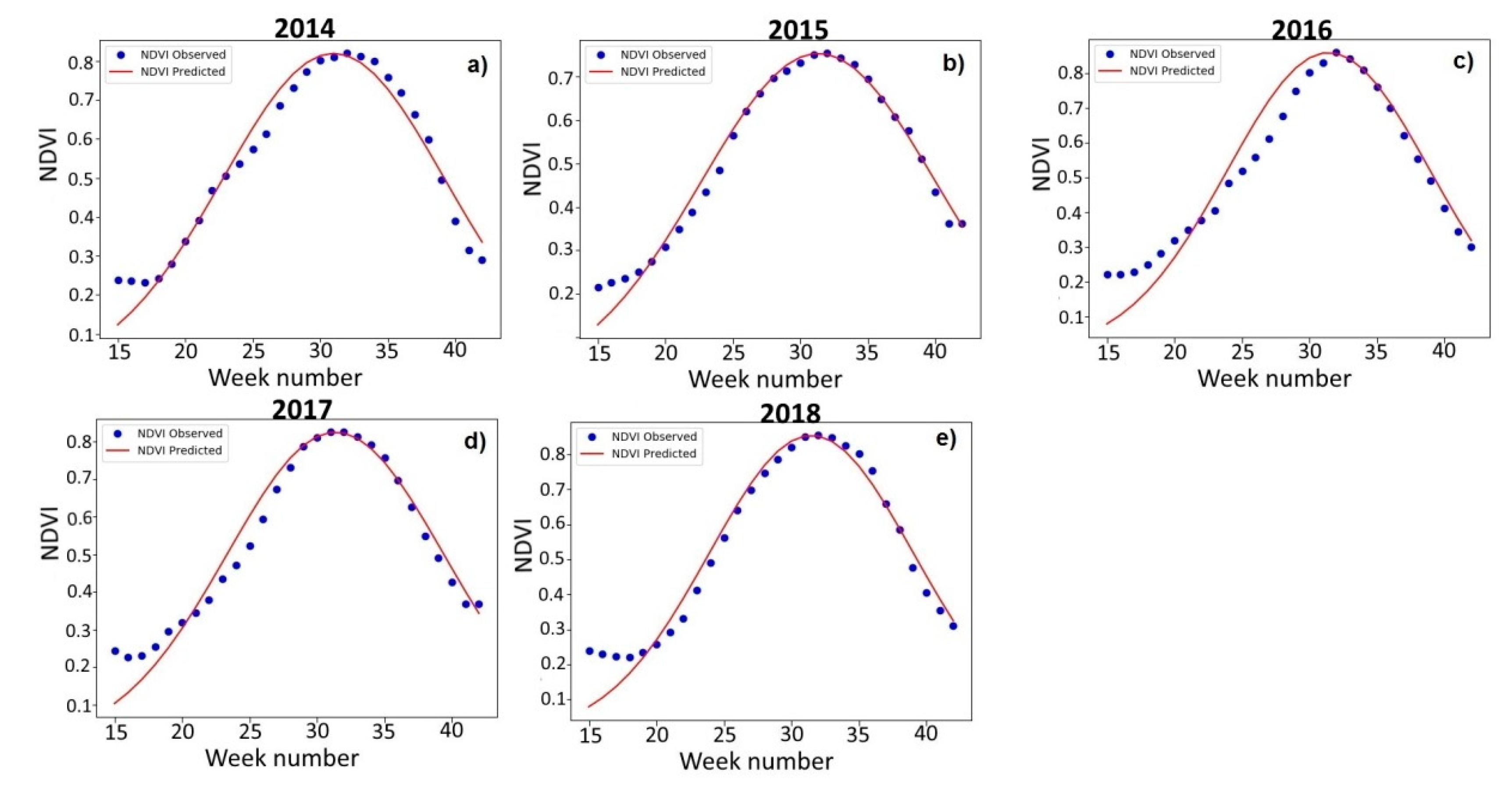
Figure 3 shows the NDVI seasonal dynamics for the experimental soybean fields from 2014 to 2018. The average soybean weekly NDVI was calculated as the weighted sum of all soybean fields’ NDVI values (taking into account the area of the fields). Then, we determined the maximum NDVI value for each season using these average NDVI series. It was found that the average expressed maximum for soybeans fell on the 31st and 32nd calendar weeks (corresponding to the last decade of July to the first decade of August). The selected Gaussian function satisfactorily approximated the initial NDVI series. Parameter c in the researched years ranged from 7.5 to 8.7, and parameter b from 31.0 to 31.5 (

Table 2. Parameters of the NDVI curves, the maximum NDVI, mean absolute percentage error (MAPE), and root-mean-square error (RMSE) for the experimental soybean fields in the Khabarovsk District in 2014–2018.

	2014	2015	2016	2017	2018
c	8.2	8.7	7.5	8.0	7.6
b	31.0	31.3	31.4	31.4	31.5
$NDV{I}_{\max }^{pred}$	0.819	0.753	0.858	0.825	0.852
$NDV{I}_{\max }^{obs}$	0.819	0.753	0.859	0.826	0.854
MAPE, %	8.5	6.0	13.9	10.2	10.9
RMSE	0.043	0.029	0.063	0.048	0.05

). It is remarkable that 2015 is characterized by the maximum peak width and the lowest maximum NDVI values. In contrast, in 2016 and 2018, the maximum NDVI values, respectively, were 0.859 and 0.854, while the b values were minimal—7.5 and 7.6. The approximation accuracies in 2014 and 2015 were, respectively, 8.5% and 6.0%; in 2016, 13.9%; and in 2017 and 2018, 10.2% and 10.9%. Approximation RMSE varied from 0.029 in 2015 to 0.063 in 2016.

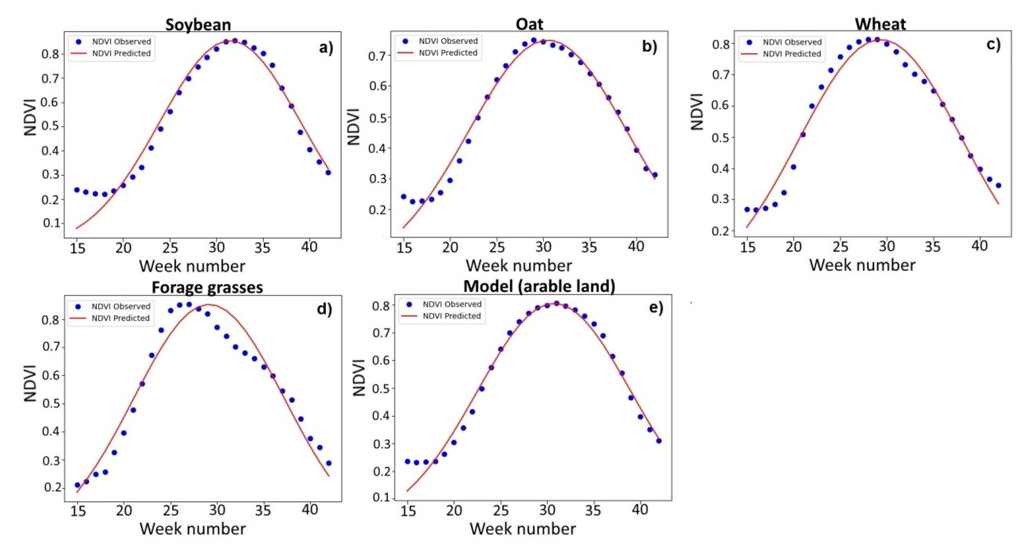
Figure 4 shows the seasonal NDVI approximating graphs for the main crops of the study area in 2018 (obtained from the experimental fields). It is easy to notice that the seasonal NDVI variation for oat and wheat corresponds to the Gaussian curve, while the corresponding curve for forage grasses has a displaced maximum. The figure also shows the seasonal NDVI variation for a model that takes into account the structure of the arable land in the Khabarovsk District. We multiplied the NDVI values by a fraction of a particular crop-sown area from the total area of the arable fields in the region and then summarized them for all of the researched cultures to calculate the weekly NDVI composites in the model of the arable land.

As follows from

Table 3. Parameters of the NDVI seasonal variation curves, the maximum NDVI values, and the errors for crops grown in the experimental fields in the Khabarovsk District in 2018.

	Soybean	Spring Wheat	Oat	Forage Grasses	Model (Arable Land)
c	7.6	8.7	8.5	8.1	9.2
b	31.5	29.4	30.5	29.2	30.4
$NDV{I}_{\max }^{pred}$	0.852	0.811	0.747	0.852	0.805
$NDV{I}_{\max }^{obs}$	0.854	0.812	0.748	0.852	0.806
MAPE, %	10.9	6.5	6.2	9.1	6.6
RMSE	0.05	0.035	0.029	0.052	0.032

, the b values in 2018 for wheat and forage grasses were 29.4 and 29.2, respectively, while for oat and the arable land model, they were 30.5 and 30.4. The range of c values for the different crops varied from 7.6 to 8.7, and for the arable land model, the corresponding parameter was 9.2. The Gaussian bell’s widening in the arable land model is explainable because different crops are characterized by different growing season lengths and different maximum NDVI values, which, accordingly, contribute to the peak’s expansion and the maximum decrease relative to the leading crop, while the total area under the curve can remain at the individual crop level. The model MAPE for spring wheat, oat, and arable land at the end of 2018 did not exceed 7%; the corresponding indicator for forage grasses was 9.1%, and for soybean was 10.9%. The RMSE for the arable land of the Khabarovsk District was 0.032.

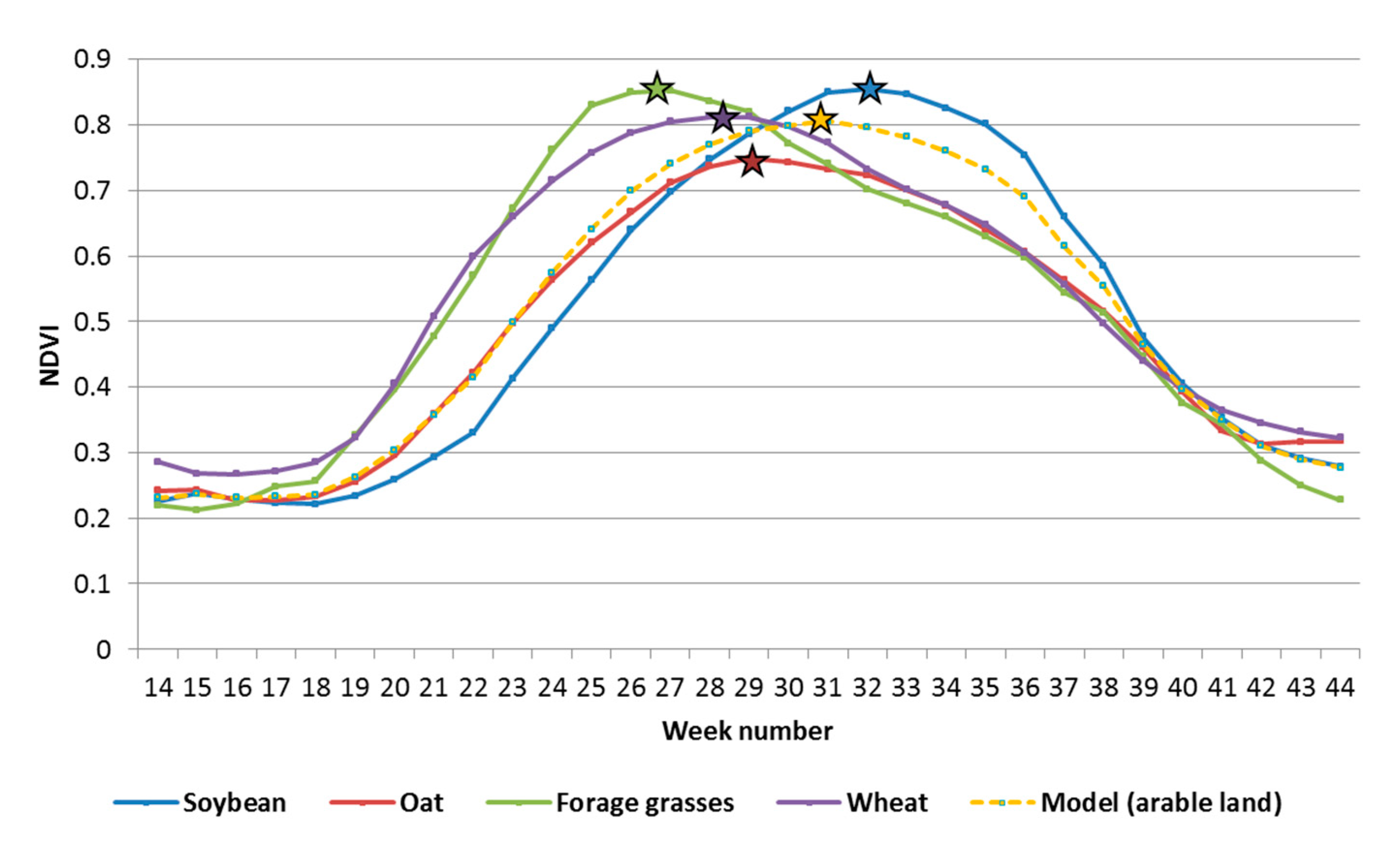
In 2018, the maximum NDVI values for soybeans corresponded to the 32nd calendar week; for oat, to the 29th week; for wheat, to the 28th week; and for forage grasses, to the 26th week (i.e., the third decade of June) (Figure 5). Thus, the maximum NDVI values for different crops vary noticeably in timing (from June 20 to August 10, i.e., for more than a month and a half). The maximum NDVI value was assumed to correspond to the period of the 30th and 31st calendar weeks in the arable land model. At the same time, the numerical value of the maximum NDVI for the arable land model was 0.805, which is lower than the corresponding indicator for the main crop-soybean. The NDVI_max (NDVI maximum) for soybean in 2018 was 0.852.

3.2. NDVI Seasonal Dynamics for the Arable Land in the Khabarovsk District in 2014–2018

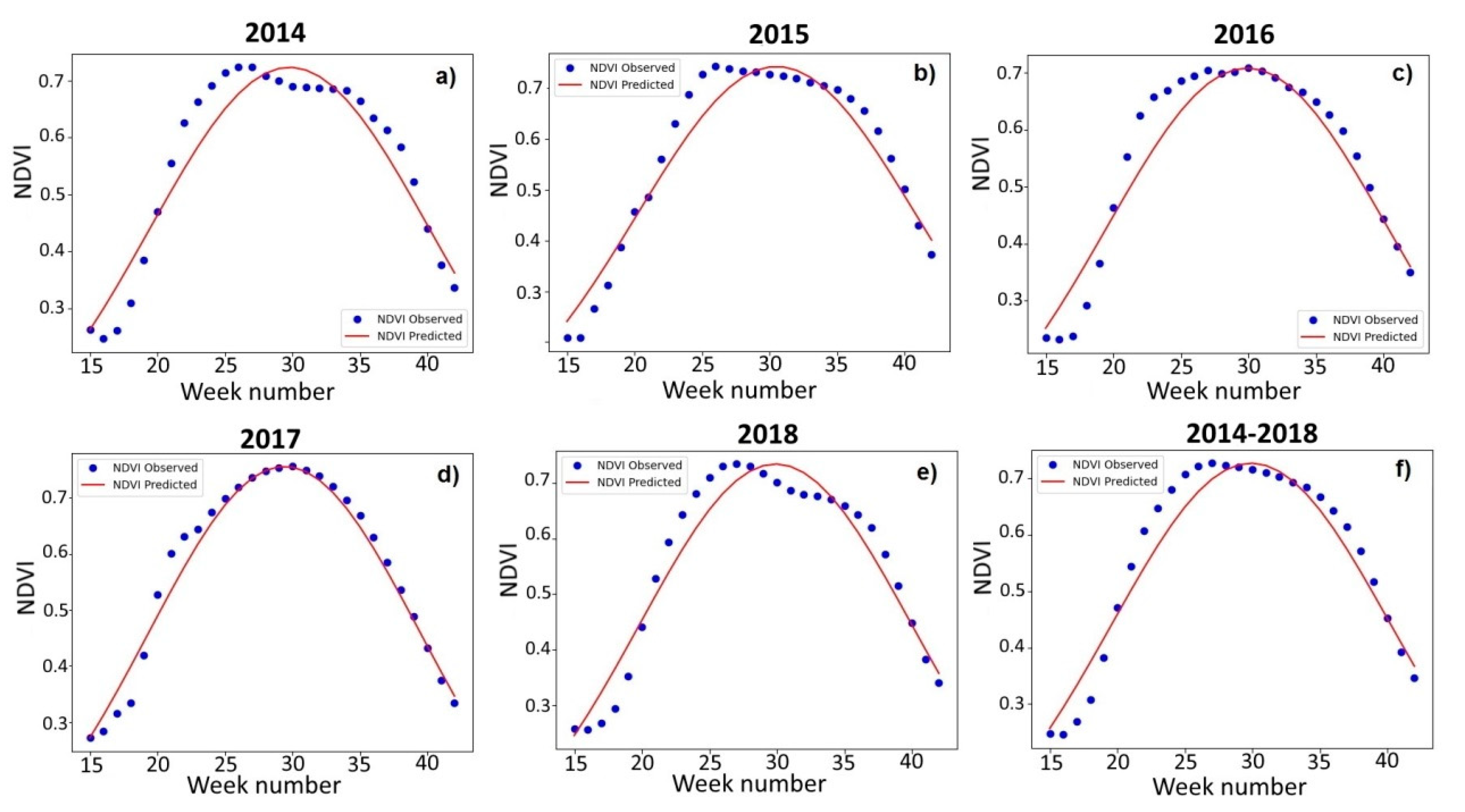
Figure 6 shows the weekly NDVI composites’ dynamics for the arable land in the Khabarovsk District in 2014–2018. The maximum value of NDVI is reached earlier than the maximum of the approximating function. This shift can be explained by errors in arable land mask generation. We suppose that natural meadows, quite widely represented in the study area, were partially erroneously classified as arable lands. From 2014 to 2018, the maximum NDVI corresponded to the 26th–30th weeks (earlier in 2014, 2015, and 2018, and later in 2016 and 2017). The average maximum for 2014–2018 fell on the 28th calendar week.

Table 4. Parameters of the NDVI approximation curves, the maximum NDVI values, and the model errors for the arable land in the Khabarovsk District in 2014–2018.

	2014	2015	2016	2017	2018	Average, 2014–2018
c	10.4	10.3	10.4	10.1	10.1	10.3
b	29.8	30.5	29.9	29.4	29.9	29.9
$NDV{I}_{\max }^{pred}$	0.723	0.742	0.708	0.755	0.734	0.727
$NDV{I}_{\max }^{obs}$	0.724	0.743	0.708	0.756	0.734	0.727
MAPE, %	7.7	6.9	7.4	3.9	6.9	6.5
RMSE	0.044	0.039	0.044	0.026	0.039	0.038

provides the parameters of the approximation curves. The b values in 2014, 2016, and 2018 were at the level of 29.8–29.9, while in 2017, it was 29.4, and in 2015, it was 30.5. Parameter c varied from 10.1 to 10.4. The calculated parameters for the averaged seasonal variation over the five years were, accordingly, 29.9 and 10.3. MAPE ranged from 3.9% in 2017 to 7.7% in 2014. The maximum NDVI value ranged from 0.708 in 2016 to 0.756 in 2017 (the variability was 2.6%, while the variability for the experimental soybean fields was 5.1%). The averaged (2014–2018) maximum NDVI value was 0.727, and MAPE was 6.5% (RMSE was 0.038).

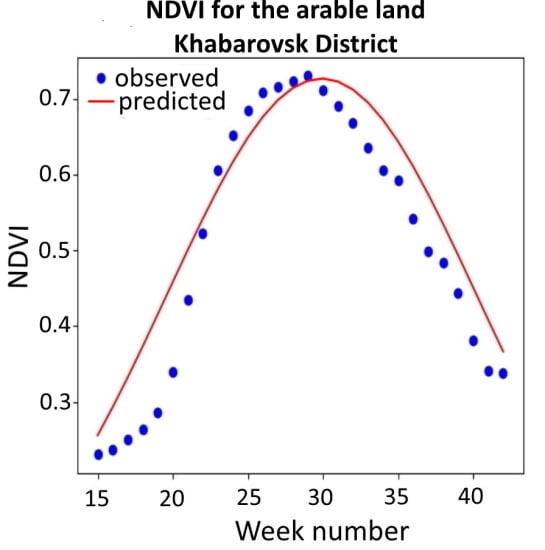
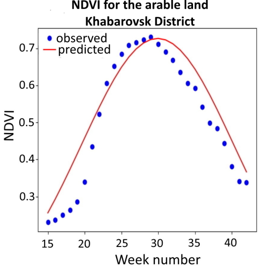
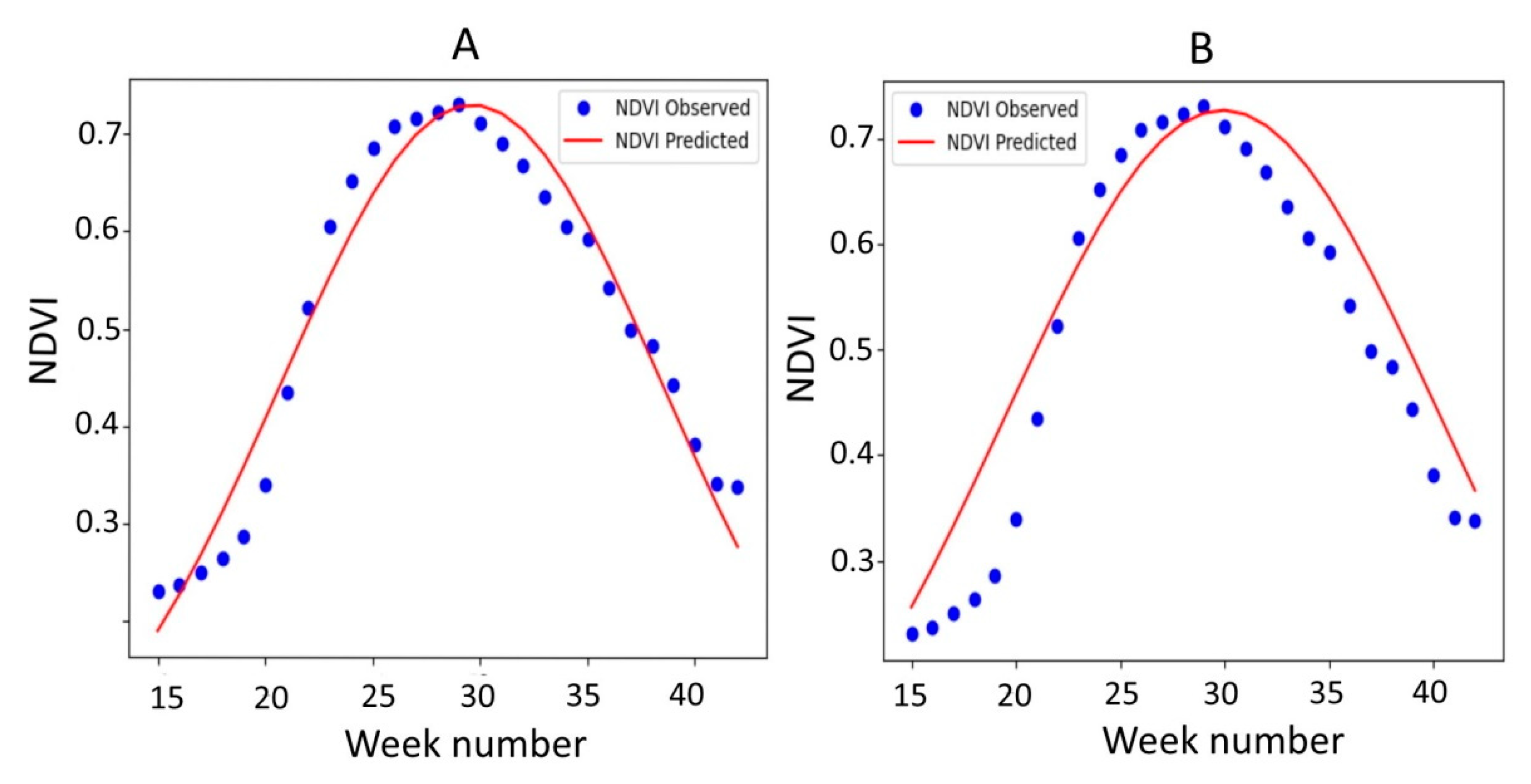
Correlation analysis showed that the maximum NDVI values (2014–2018) of the arable land in the Khabarovsk District strongly correlate with the maximum NDVI values of the experimental soybean fields (R = 0.73). Figure 7 shows the NDVI composites from the 15th to the 42nd calendar weeks, while the approximation was carried out in two ways—i.e., using the observed NDVI composites in 2019 (Figure 7A) and using the parameters of the approximating function obtained according to the averaged data for 2014–2018 (Figure 7B). The maximum NDVI was reached in the 29th calendar week and equaled 0.73. The b values were 29.6 (Figure 7A) and 29.9 (Figure 7B), while the c values were 8.9 (Figure 7A) and 10.3 (Figure 7B). MAPE (Figure 7A) was equal to 7.3%. Applying the approximating function (calculated according to the parameters of 2014–2018), MAPE increased to 12.6% (RMSE increased to 0.054), and the simulated maximum value of NDVI was 0.733. The deviation of the predicted maximum from the observed maximum was 0.4%.

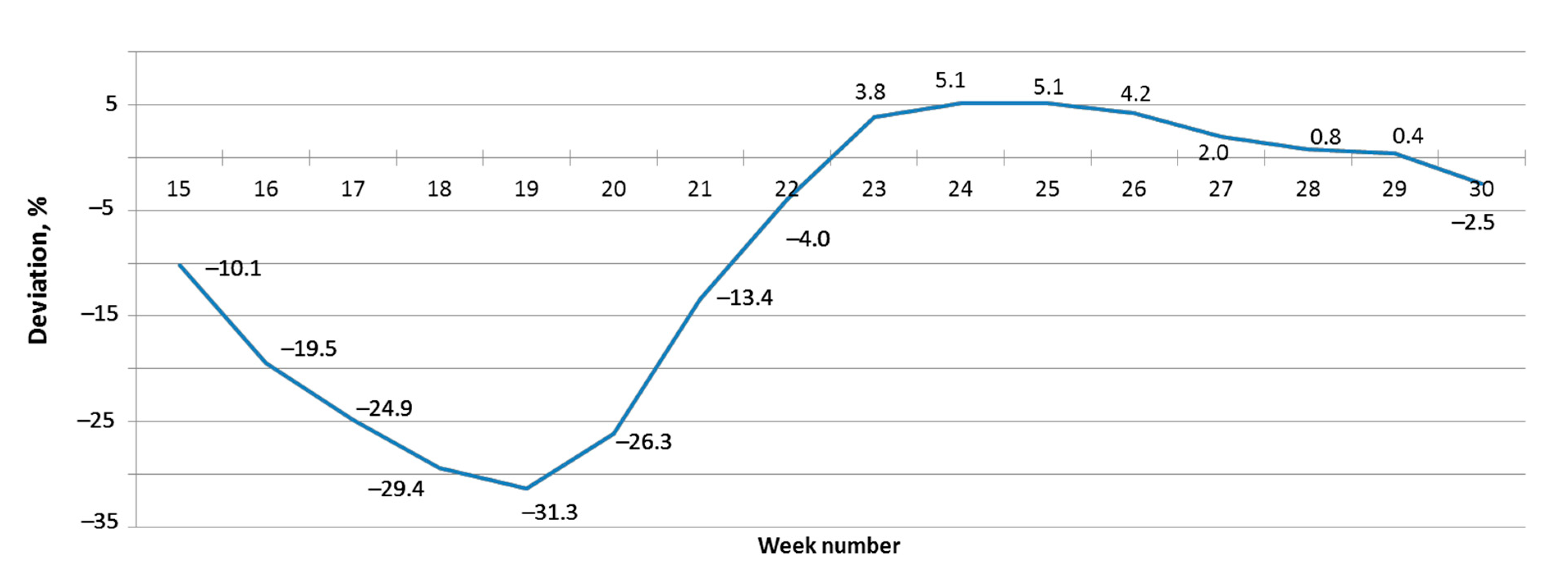
Analysis a posteriori was not the only goal of our work. For early prediction of soybean yields, it is important to predict the maximum NDVI in previous weeks. Figure 8 shows the deviation of the forecasted maximum NDVI value, calculated from the composite values of the current week, from the observed maximum. For this calculation, we used the function approximating composites averaged over 2014–2018.

In Figure 8, we can see that the accuracy of determining the maximum NDVI value becomes sufficient from the 22nd calendar week (within 5%), which corresponds to the first decade of June. When approaching the calendar maximum, the error of the maximum determination decreases to 0.4%. Due to the fact that the passage point of the maximum value cannot always be determined immediately from the seasonal NDVI schedule and that image processing is expensive, we recommend using the average value for the three weeks preceding the maximum value as the maximum NDVI. The $AP{E}_{NDV{I}_{\max }}$ in 2019 was 0.5%.

Thus, the analysis of the NDVI seasonal variation of the experimental fields and the arable land with approximation functions showed the possibility of using the maximum NDVI values of arable land in the early prediction of soybean yield.

3.3. Mathematical Model for Calculating Soybean Yield in the Khabarovsk District

During the construction of the forecast model, we calculated the values of the meteorological factors that potentially affect crop yields. It was shown that the maximum NDVI value of the arable land in the Khabarovsk District is reached by the 30th calendar week (Figure 6 and Figure 7).

Table 5. Soybean yield (y), maximum NDVI (x₁), and the meteorological indicators for the Khabarovsk District (x₂–x₆) in 2010–2018.

	y	x1	x2	x3	x4	x5	x6
2010	1.13	0.732	1.90	71.0	616.1	33.8	0.76
2011	1.19	0.742	3.03	71.0	693.9	38.0	0.76
2012	1.29	0.698	2.03	84.0	502.6	33.5	0.89
2013	1.50	0.734	2.45	72.0	414.4	36.6	0.75
2014	1.47	0.724	2.58	82.0	769.5	36.9	0.89
2015	1.19	0.743	3.07	73.0	663.3	38.1	0.78
2016	1.01	0.708	2.55	72.0	311.9	33.0	0.74
2017	1.58	0.756	1.56	75.0	707.2	31.6	0.86
2018	1.67	0.734	2.52	82.0	621.0	30.7	0.89
$\overline{x}$	1.34	0.730	2.41	75.8	588.9	34.7	0.81
σ	0.23	0.018	0.50	5.3	149.8	2.8	0.07
V, %	17.0	2.4	20.8	7.0	25.4	8.0	8.5
$\Delta \overline{x}$	0.17	0.014	0.39	4.1	115.2	2.1	0.05
min	1.01	0.698	1.56	71.0	311.9	30.7	0.74
max	1.67	0.756	3.07	84.0	769.5	38.1	0.89

provides the soybean yield estimations, the maximum NDVI values (x₁), and the values of the climatic characteristics (x₂–x₆).

Soybean yield is a fairly variable indicator, the coefficient of variation for which is 17%. The minimum value of this indicator (i.e., 1.01 t/ha) corresponds to 2016, while the maximum was observed in 2018—1.67 t/ha. The independent variables x₂ and x₄ have a high coefficient of variation. The total soil temperature (x₄) in the first 30 weeks of 2014 was 2.5 times higher than the same value in 2016 (769.5 °С and 311.9 °С, respectively). The maximum NDVI values have the least variation—2.4%—while the variability of x₃, x₅, and x₆ is in the range of 7–8.5%. In general, 2010, 2011, 2013, and 2015–2017 are characterized by a late start to the growing season (x₃ ranged from 71 to 75 days). For 2012, 2014, and 2018, x₃ (growing duration) ranged from 82 to 84 days. Similarly, the variable x₆ (photosynthetically active radiation) changed during the study period. High PAR values were observed in 2012, 2014, and 2017–2018 and ranged from 0.86 to 0.89 GJ∙m². The highest values of the indicators characterizing humidity/aridity were observed in 2011 and 2015. The average relative soil moisture (x₅) was 38.0% and 38.1%, and the Selyaninov hydrothermal coefficient (x₂) was 3.03 and 3.07, respectively.

The analysis showed that a number of the variables share a certain relationship, suggesting their exclusion from the regression model.

Table 6. Correlation matrix for the dependent and independent variables (significant coefficients (p < 0.05) are highlighted).

	y	x1	x2	x3	x4	x5	x6
y	1.00	0.31	−0.17	0.44	0.28	−0.28	0.44
x1	0.31	1.00	0.14	−0.18	0.37	0.20	−0.03
x2	−0.17	0.14	1.00	−0.09	0.22	0.56	−0.17
x3	0.44	−0.18	−0.09	1.00	0.32	−0.26	0.73
x4	0.28	0.37	0.22	0.32	1.00	0.11	0.28
x5	−0.28	0.20	0.56	−0.26	0.11	1.00	−0.17
x6	0.44	−0.03	−0.17	0.73	0.28	−0.17	1.00

provides the Kendall rank correlation coefficients for the dependent and independent variables of the regression model. A rather high correlation coefficient value can be observed between the indices x₃ and x₆ (τ = 0.73), and x₂ and x₅ (τ = 0.56). Thus, it is advisable to leave only one of the two variables characterizing the degree of aridity (x₂) and to exclude x₆ from the regression model. It is also possible to preliminarily characterize the impact of the indicators on soybean yield using the correlation table. Thus, the maximum NDVI value, the duration of the growing season, the total temperature of the soil, and the PAR are all directly related to the average crop yield. Conversely, soil moisture and SHC are inversely related to soybean yield.

Variables x₅ and x₆ were excluded during the correlation analysis, and variables x₂ and x₄ were automatically excluded during stepwise model construction as insignificant indicators. As a result, the multiple regression equation, which characterizes the dependence of soybean yield in the Khabarovsk District on the variables included in the model, constructed according to the data of 2010–2018, has the following form:

$$y=-8.24+9.39x_1+0.036x_3.$$

(12)

The model’s coefficient of determination (R²) is 0.72. The standardized values of the regression coefficients are approximately equal, which indicates the same effect of the predictors on soybean yield (

Table 7. Regression summary for the dependent variables (b* is normalized regression coefficients).

	b*	Std.Err. of b*	b	Std.Err. of b	t (6)	p-Value
Intercept			−8.24543	2.644295	−3.1182	0.020632
x1	0.738891	0.23912	9.38573	3.037413	3.09004	0.021387
x3	0.847303	0.23912	0.03603	0.010169	3.54342	0.012168

). All of the coefficients of the regression equation are significant (p < 0.05).

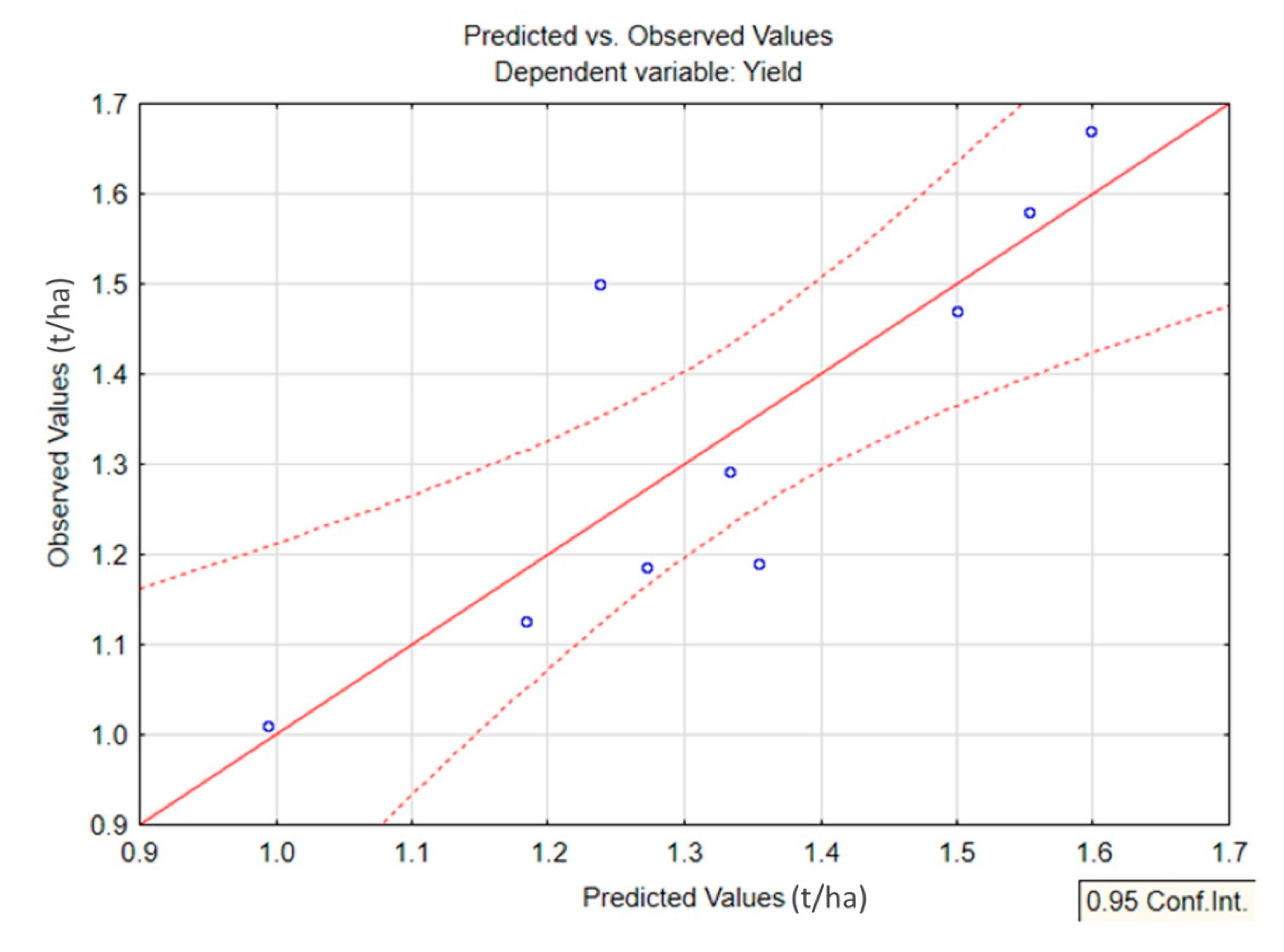
An analysis of the results showed that the predicted values for most of the observed years are within the confidence interval (γ = 0.95) for the actual soybean yield (Figure 9). The largest deviation was observed in 2013, which is due, possibly, to an inaccurate estimate of soybean yield in the Khabarovsk District, caused by the largest flood in the history of observations of the Amur River. As a result of the flood, 16,000 hectares of farmland in the Khabarovsk Territory were affected, including the lands of the Big Ussuriysky Island (90% flooded). The final statistics of the Federal State Statistics Service of Russia in 2013 were affected by the high proportion of soybean fields in the non-flooded sown areas of the Khabarovsk Territory.

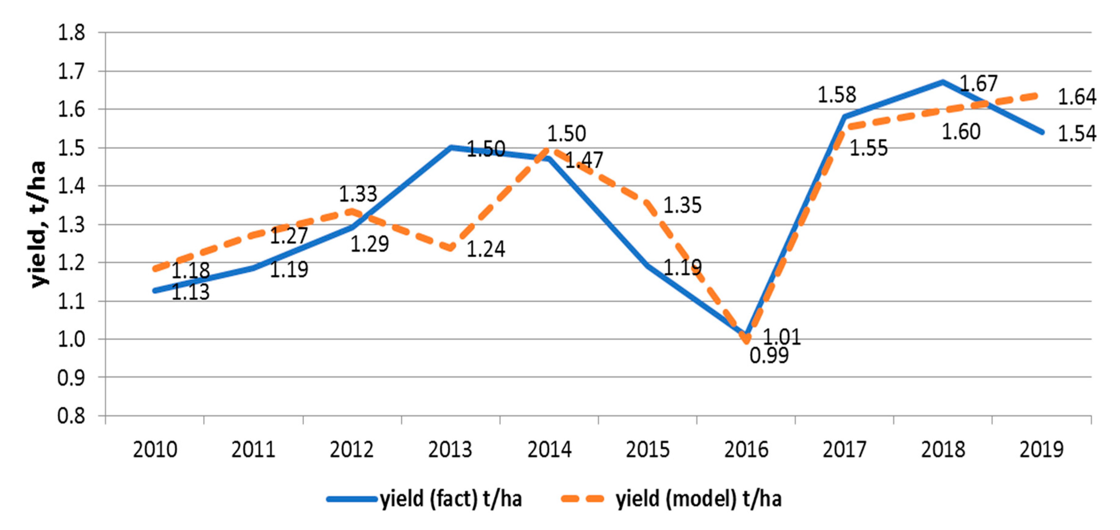
Figure 10 shows the actual and estimated values of the average soybean yield for 2010–2018. Moreover, we forecasted soybean yield in the Khabarovsk region in 2019 using the regression model. The predicted and real values of soybean yield in 2019 are also reflected in Figure 10. The MAPE of the model was 6.2%, the RMSE was 0.13 t/ha, and the APE was 6.3% (using the actual values of the maximum NDVI). Thus, the developed model shows fairly high accuracy when calculating soybean yield in the Khabarovsk District for 2018.

The regression model had high accuracy, as evidenced in R²_cv, RMSE_cv, and MAPE_cv values obtained using a leave-one-year-out (2010–2019) cross-validation procedure (

Table 8. Cross-validated coefficient of determination (R²_cv), root-mean-square error (RMSE_cv), mean absolute percentage error (MAPE_cv), and absolute percentage error (APE_cv), calculated in a one-leave-out cross−validated approach for the regression model.

	R2cv	RMSEcv (t/ha)	MAPEcv, %	APEcv, %
2010	0.70	0.11	6.1	3.5
2011	0.73	0.11	5.8	7.9
2012	0.73	0.12	6.5	4.9
2013	0.81	0.07	4.0	22.7
2014	0.72	0.12	6.5	1.2
2015	0.79	0.10	5.1	18.3
2016	0.62	0.12	6.4	2.2
2017	0.70	0.11	6.1	2.9
2018	0.68	0.11	5.7	8.2
2019	0.72	0.11	6.2	5.8
$\overline{x}$		0.11	5.9	7.8
$\Delta \overline{x}$		0.01	0.6	5.1

). APE_cv was mainly within 8% (except 2013 and 2015).

We evaluated model accuracy using approximated NDVI maxima to solve the problem of early forecasting and calculated the NDVI maxima from the 22nd to the 30th calendar weeks in 2010–2019 using the Gaussian approximation function.

Table 9. Average RMSE and APE yield values, calculated using approximated NDVI maxima for 22 (June 1)–30 (July 30) calendar weeks in the Khabarovsk District (2010–2019).

Week	22	23	24	25	26	27	28	29	30
RMSE	0.77	0.74	0.67	0.38	0.33	0.21	0.18	0.16	0.15
APE Yield,%	50.2	51.4	47.2	40.4	29.9	19.2	9.9	8.5	7.6

provides an estimate of the model accuracy using the RMSE and APE, where the predicted NDVI values were used as an independent model variable in regression equations for each year from 2010 to 2019. Regression equations were obtained using a leave-one-year-out cross-validation procedure.

The model’s average APE increased from 5.9% (actual average NDVI maxima) to 7.6–9.9% (predicted NDVI maxima, calculated using NDVI 28th, 29th, 30th weeks). The average RMSE increased from 0.11 t/ha to 0.15–0.18 t/ha.

Table 10. NDVI values (observed in ith week); NDVI maxima, soybean yield, and absolute percentage errors in 2019 in the Khabarovsk District, calculated using the approximating function in the 22nd (June 1) to 30th (July 30) calendar weeks.

Week	22	23	24	25	26	27	28	29	30
$NDV{I}_i$	0.523	0.606	0.652	0.686	0.709	0.716	0.724	0.730	0.712
$NDV{I}_{\max }^{pred}$	0.701	0.758	0.768	0.768	0.761	0.745	0.736	0.733	0.712
APE NDVI, %	4.0	3.8	5.1	5.1	4.2	2.0	0.8	0.4	2.5
Calculated Yield, t/ha	1.36	1.90	1.99	1.99	1.93	1.77	1.69	1.66	1.47
APE Yield,%	11.5	23.4	29.0	29.0	25.1	15.2	9.7	8.0	4.3

presents the calculated NDVI maxima for i weeks in 2019, as well as the corresponding yield values. The parameters of the Gaussian approximation function (average for 2014−2018) are given in Table 4.

The calculated crop yields ranged from 1.36 to 1.99 t/ha for different weeks. Prediction error (APE) in the 23rd to 26th weeks ranged from 23% to 29%, did not exceed 10% in the 28th and 29th weeks, and was 4.3% in the 30th week.

3.4. Soybean Yield Prediction in Other Municipalities of Far East Based on Proposed Model

We predicted soybean yield in 11 soybean-producing municipalities of the Russian Far East, using our regression model with the maximum NDVI value and the growing season duration (as of 30 weeks) as independent variables.

Table 11. Average RMSE results for the different municipalities in the Russian Far East (2010–2018). Significant results highlighted bold, insignificant highlighted italics.

Region	District	RMSE (t/ha)	R2	p
Khabarovsk Territory	Khabarovsk	0.11	0.72	0.02
	Vyasemskiy	0.09	0.76	0.03
	Lazo	0.10	0.15	0.06
Jewish Autonomous Region	Oktyabrskiy	0.06	0.74	0.07
	Leninskiy	0.15	0.38	0.39
Amur Region	Tambovskiy	0.05	0.94	0.01
	Mikhailovskiy	0.09	0.8	0.04
Primorskiy Territory	Khorolskiy	0.13	0.32	0.32
	Khankaiskiy	0.11	0.68	0.03
	Mikhaylovskiy	0.16	0.01	0.95
	Chernigovskiy	0.16	0.12	0.69

provides the average errors of forecasting, the R² values, and the p-values.

The RMSE, the R² values, and the p-values for some regions (i.e., the Khabarovsk, Vyasemskiy, Tambovskiy, Mikhailovskiy, and Khankaiskiy districts) are quite satisfactory. The early forecasting method development for soybean and other crops for different territories is a priority area for future research.

4. Discussion

Various researchers have investigated the seasonal course of NDVI, as well as other vegetative indices, for different crops obtained using remote sensing data. For example, the use of the asymmetric Gaussian and double logistical functions for modeling seasonal changes in vegetation indices was considered in Reference [44]. The paper [45] presented the application of the iterative logistic fitting method for Enhanced Vegetation Index (EVI) modeling in grasslands. Seo et al. [46] used two logistic curves (one for the early and one for the later parts of the growth period) for corn and soybean NDVI approximation. Berger et al. [47] presented NDVI prediction according to historical data using soybean in Uruguay as an example. In their study, a set of fields, each at least 250 ha in size, were studied; to approximate the seasonal course of NDVI, the authors used two models: one with a polynomial and the other a double logistic function interpolation.

The RMSE for the studied soybean fields was 0.15 for the polynomial approximation and 0.11 for the logistic approximation. All of the RMSEs in our model using Gaussian as an approximating function are below 0.1, which is a fairly good result. The time interval for approximation in our model from the 15th to the 42nd calendar weeks (196 days) approximately corresponds to the time interval considered in [47]—from November 11 to May 5 of the next year (adjusted for the season in the Southern Hemisphere). Consideration of the arable land as a whole (instead of as individual fields) contributed to the superiority of our model. We suppose that the main goal of approximation is to determine the maximum NDVI value as accurately as possible in order to enable early forecasting. Therefore, as a further development of our work, the phenological stages of soybean, including the emergence, flowering, and maturation dates of the soybean, should be studied. Papers [48,49] calculated the relationship of the quantitative and qualitative indicators of soybean with vegetation indices using the remote sensing data of different phenological stages.

In our study, we used the maximum value of the NDVI index as one of the independent variables of the model. However, a reasonable question arises: Is it not more appropriate to use the NDVI values of other days (weeks) in early yield forecasting? This is most reasonable for winter crops because their first maximum is observed in early spring [50]. On the other hand, some researchers have noted that the best results in predicting crop yields may not be achieved during the passage of the maximum NDVI value. Magney et al. [51] showed that the best results for predicting wheat yields are observed over two periods—on days 37–46, and also on days 75–85 after the emergence of seedlings. Ren et al. [52] compared regression models using NDVI values in different weeks of April and May. They showed that errors of the predicted yield using MODIS–NDVI varied between 4.62% and 5.40% depending on the NDVI values, as well as that the average RMSE was 0.21 t/ha. Lopresti et al. [53] estimated wheat yields in Argentina using NDVI values between the 289th and 305th calendar days of the year, which in the Southern Hemisphere corresponds to March in the Northern Hemisphere, and the RMSE varied from 0.40 to 0.46 t ha⁻¹ for the different regions of Argentina. Using early NDVI values in soybean analysis is, in our opinion, quite a difficult task.

Thus, the use of NDVI before it reaches its maximum value significantly decreases the accuracy of the model. The solution to this problem could be a promising research area. In general, an analysis of recent works devoted to assessing crop yields at the region or municipality level using remote sensing data showed that the developed model has enough accuracy. Thus, in Reference [54], the average error of the regression model for corn yield prediction in the period of 2010–2014 was 4.5%. Neravuori et al. proposed a method for predicting crop yields in mixed-crop fields (the predominant crop being mainly wheat) using vegetation indices in the model during the early period of the growth season (i.e., in June) [55]. The MAPE of this model was 8.8%; however, when using data acquired later in July and August, the MAPE increased to 12.6%.

Wei et al. [56] showed an approach combining the SIMDualKc water balance model and the Stewart water-yield model for soybean. The accuracy of this model is of particular interest because the work was performed in Northeast China—that is, in the adjacent region to the Russian Far East. The RMSE of the model was 0.38 t/ha—about 11.5% of the maximum observed yield. Sacamoto [57] compared three methods for assessing crop yields, that is, linear regression, polynomial regression (PM), and the random forest (RF) method, where temperature, precipitation, and shortwave radiation were used in addition to NDVI. The obtained equations were used to estimate soybean yield in a few regions of Nebraska (USA). Averaged by regions, the RMSE was 0.28 t/ha for PM and 0.21 t/ha for RF.

Other meteorological factors can be used to improve the yield forecasting model. For example, in Reference [58], atmospheric pressure was used in wheat yield prediction in China. The influence of air temperature in the surface layer on wheat productivity was considered in References [20,59]. However, the experiments for the Khabarovsk District showed that these climatic indicators do not significantly affect soybean yield. Both of these indicators are inversely correlated with the maximum NDVI value (which prevents their use in the model). Such a negative correlation can be explained by the fact that high atmospheric pressure, which causes a lack of precipitation, high temperature, and hot weather in late spring and early summer, leads to destructive effects on plant maturation. However, at the same time, they do not correlate with crop yield at the end of the year.

Various climatic indices are used for yield modeling; for example, Pacific Decadal Oscillation (PDO) and MEI (Multivariate El Niño/Southern Oscillation index) [60] and monthly drought index (DI) [61]. In agrometeorological studies in Russia and the Commonwealth of Independent States (CIS), the most commonly used indices are the Selyaninov hydrothermal coefficient (SHC), the climate biological effectiveness (CBE), and the Budyko dryness index (BDI) [62,63]. Correlation analysis showed that all of the listed climatic indices are significantly (p < 0.05) correlated with each other; therefore, it was decided to choose just one of the indices—the SHC. During our research, the SHC index (for the first 30 weeks of the year) was excluded at the stage of regression equation building. Application of the other indices gives similar results: The corresponding variables are excluded during stepwise regression process.

In Reference [45], it was stated that the addition of various soil characteristics (i.e., soil temperature and moisture in different layers) increases the determination coefficient of the wheat yield regression model by 0.12. In this work, the temperature and soil moisture in the upper layer (at a depth of 10 cm) were previously considered as independent variables. Both of these indicators were excluded from the model during the model building process. Using soil temperature and soil moisture in a 10–40 cm layer instead of similar indicators for the top layer allows to build an alternative model for early yield prediction:

$$y=-4.98+7.13x_1+0.002x_2,$$

(13)

where x₁ is the maximum NDVI value, and x₂ is the total soil temperature in the 10–40 cm layer during the vegetation season (before the 30th week). The model’s determination coefficient (R² = 0.68) is slightly less than the corresponding coefficient for our equation from Section 3. Thus, this equation proves the relationship between soil temperature in deep layers and soybean yield. Further study of the influence of soil characteristics on crop yields looks promising.

5. Conclusions

The present study was devoted to the early forecasting of crop yields in a particular region or municipality using remote sensing and reanalysis data. A soybean yield regression model was built, where the maximum weekly composites of NDVI arable fields and the duration of the growing season from the 1st to the 30th calendar weeks were included as independent variables. The advantage of this approach lies in the possibility of using data obtained from the mask of arable fields and, therefore, in the absence of a laborious (and sometimes impossible) definition of separate cultures. The model was preliminarily evaluated using experimental fields, constructed in accordance with the structure of the arable land in the Khabarovsk District. Using the Gaussian function to approximate the seasonal NDVI variation allowed us to determine the calendar weeks with the maximum NDVI for different crops and for the arable land of the Khabarovsk District. It is proposed to use the parameters of the approximating function of five previous years to predict NDVI before reaching the extremum. The RMSE of the approximating model in 2019 was 0.054, and the error of maximum prediction did not exceed 0.5%.

The error of the regression model according to 2010–2018 was 6.2%, and the RMSE was 0.13 t/ha. Meanwhile, the forecast error for 2019 was 6.3%. The analysis showed that the accuracy of the developed model is quite sufficient for forecasting in agriculture. It is also possible to use the developed model for earlier forecasting, starting from the 28th calendar week—in this case, the RMSE model increased to 0.18 t/ha. A preliminary model assessment for the analysis of other soybean-producing regions in the Far East showed that the RMSE for soybean yield prediction varied from 0.05 to 0.16 t/ha.

References

- Gaso, D.V.; Berger, A.; Ciganda, V. Predicting wheat grain yield and spatial variability at field scale using a simple regression or a crop model in conjunction with Landsat images. Comput. Electron. Agric. 2019, 159, 75–83. [Google Scholar] [CrossRef]
- Becker-Reshef, I.; Franch, B.; Barker, B.; Murphy, E.; Santamaría-Artigas, A.; Humber, M.; Skakun, S.; Vermote, E. Prior Season Crop Type Masks for Winter Wheat Yield Forecasting: A US Case Study. Remote Sens. 2018, 10, 1659. [Google Scholar] [CrossRef] [Green Version]
- Nicola, M.; Alsafi, Z.; Sohrabi, C.; Kerwan, A.; Al-Jabir, A.; Iosifidis, C.; Agha, M.; Agha, R. The Socio-Economic Implications of the Coronavirus and COVID-19 Pandemic: A Review. Int. J. Surg. 2020, 78, 185–193. [Google Scholar] [CrossRef]
- Lai, Y.R.; Pringle, M.J.; Kopittke, P.M.; Menzies, N.W.; Orton, T.G.; Dang, Y.P. An empirical model for prediction of wheat yield, using time-integrated Landsat NDVI. Int. J. Appl. Earth Obs. Geoinf. 2018, 72, 99–108. [Google Scholar] [CrossRef]
- Prabhakara, K.; Hively, W.D.; McCarty, G.W. Evaluating the relationship between biomass, percent groundcover and remote sensing indices across six winter cover crop fileds in Maryland, United States. Int. J. Appl. Earth Obs. Geoinf. 2015, 39, 88–102. [Google Scholar] [CrossRef] [Green Version]
- Liu, J.; Shang, J.; Qian, B.; Huffman, T.; Zhang, Y.; Dong, T.; Jing, Q.; Martin, T. Crop Yield Estimation Using Time-Series MODIS Data and the Effects of Cropland Masks in Ontario, Canada. Remote Sens. 2019, 11, 2419. [Google Scholar] [CrossRef] [Green Version]
- Chipanshi, A.; Zhang, Y.; Kouadio, L.; Newlands, N.; Davidson, A.; Hill, H.; Warren, R.; Qian, B.; Daneshfar, B.; Bedard, F.; et al. Evaluation of the integrated Canadian crop yield forecaster (iICCYF) model for in-season prediction of crop yield across the Canadian agricultural landscape. Agric. For. Meteorol. 2015, 206, 137–150. [Google Scholar] [CrossRef] [Green Version]
- Huffman, T.; Liu, J.; Green, M.; Coote, D.; Li, Z.; Liu, H.; Liu, T.; Zhang, X.; Du, Y. Improving and evaluating the soil cover indicator for agricultural land in Canada. Ecol. Indic. 2015, 48, 272–281. [Google Scholar] [CrossRef]
- Mkhabela, M.S.; Bullock, P.; Raj, S.; Wang, S.; Yang, Y. Crop yield forecasting on the Canadian prairies using MODIS NDVI data. Agric. For. Meteorol. 2011, 151, 385–393. [Google Scholar] [CrossRef]
- López-Lozano, R.; Duveiller, G.; Seguini, L.; Meroni, M.; García-Condado, S.; Hooker, J.; Leo, O.; Baruth, B. Towards regional grain yield forecasting with 1km-resolution EO biophysical products: Strengths and limitations at Pan-European level. Agric. For. Meteorol. 2015, 206, 12–32. [Google Scholar] [CrossRef]
- Kowalik, W.; Dabrowska-Zielinska, K.; Meroni, M.; Raczka, T.U.; de Wit, A. Yield estimation using SPOT-VEGETATION products: A case study of wheat in European countries. Int. J. Appl. Earth Obs. 2014, 32, 228–239. [Google Scholar] [CrossRef]
- Bolton, D.; Friedl, M. Forecasting crop yield using remotely sensed vegetation indices and crop phenology metrics. Agric. For. Meteorol. 2013, 173, 74–84. [Google Scholar] [CrossRef]
- Johnson, D.M. A comprehensive assessment of the correlations between field crop yields and commonly used MODIS products. Int. J. Appl. Earth Obs. 2016, 52, 65–81. [Google Scholar] [CrossRef] [Green Version]
- Toshichika, I.; Shin, Y.; Kim, W. Global crop yield forecasting using seasonal climate information from a multi-model ensemble. Clim. Serv. 2018, 11, 13–23. [Google Scholar]
- Onojeghuo, A.; Blackburn, G.; Huang, J. Applications of satellite ‘hyper-sensing’ in Chinese agriculture: Challenges and opportunities. Int. J. Appl. Earth Obs. Geoinf. 2018, 64, 62–86. [Google Scholar] [CrossRef] [Green Version]
- Zhu, C.; Lu, D.; de Castro Victoria, D.; Dutra, L. Mapping Fractional Cropland Distribution in Mato Grosso, Brazil using time series MODIS Enhanced Vegetation Index and Landsat Thematic Mapper data. Remote Sens. 2016, 8, 22. [Google Scholar] [CrossRef] [Green Version]
- Cunha, M.; Marçal, A.; Silva, L. Very early prediction of wine yield based on satellite data from VEGETATION. Int. J. Remote Sens. 2010, 31, 3125–3142. [Google Scholar] [CrossRef]
- Saeed, U.; Dempewolf, J.; Becker-Reshef, I.; Khan, A.; Ahmad, A.; Wajid, S.A. Forecasting wheat yield from weather data and MODIS NDVI using Random Forests for Punjab province, Pakistan. Int. J. Remote Sens. 2017, 38, 4831–4854. [Google Scholar] [CrossRef]
- de la Casaa, A.; Ovandoa, G.; Bressanini, L. Soybean crop coverage estimation from NDVI images with different spatial resolution to evaluate yield variability in a plot. ISPRS J. Photogramm. Remote Sens. 2018, 146, 531–547. [Google Scholar] [CrossRef]
- Balaghi, R.; Tychon, B.; Eerens, H. Empirical regression models using NDVI, rainfall and temperature data for the early prediction of wheat grain yields in Morocco. Int. J. Appl. Earth Obs. Geoinf. 2008, 10, 438–452. [Google Scholar] [CrossRef] [Green Version]
- Maas, S.J. GRAMI: A Crop Model Growth Model That Can Use Remotely Sensed Information; USDA-ARS: Washington, DC, USA, 1992; p. 78.
- Aseeva, T.; Karacheva, G.; Lomakina, I. Forming the Productivity of Spring and Winter Wheat in the Conditions of the Middle Priamurye Region. Russ. Agric. Sci. 2018, 44, 113–117. [Google Scholar] [CrossRef]
- Hasbiullina, O.; Mudrik, N.; Butovets, E. Analysis of soybean selective breeding material at the Primorskiy Research Institute of Agriculture. Bull. Altai State Agrar. Univ. 2013, 2, 28–31. (In Russian) [Google Scholar]
- Savin, I.Y.; Bartalev, S.A.; Loupian, E.A.; Tolpin, V.A.; Khvostikov, S.A. Crop yield forecasting based on satellite data: Opportunities and perspectives. Sovr. Probl. DZZ Kosm. 2010, 7, 275–285. [Google Scholar]
- Bereza, O.; Strashnaya, A.; Loupian, E. On the possibility to predict the yield of winter wheat in the Middle Volga region on the basis of integration of land and satellite data. Sovr. Probl. DZZ Kosm. 2015, 12, 18–30. [Google Scholar]
- Savin, I.; Chendev, Y. Reasons for long-term dynamics of NDVI (MODIS) averaged for arable lands of municipalities of Belgorod region. Sovr. Probl. DZZ Kosm. 2018, 15, 137–143. [Google Scholar] [CrossRef]
- Stepanov, A.; Aseyeva, T.; Dubrovin, K. The influence of climatic characteristics and values of NDVI at soybean yield (on the example of the districts of the Primorskiy region). Agrar. Bull. Urals. 2020, 1, 10–20. [Google Scholar] [CrossRef] [Green Version]
- Liu, X.; Jin, J.; Wang, G.; Herbert, S.J. Soybean yield physiology and development of high-yielding practices in Northeast China. Field Crops Res. 2008, 105, 157–171. [Google Scholar] [CrossRef]
- Rembold, F.; Atzberger, C.; Savin, I.; Rojas, O. Using Low Resolution Satellite Imagery for Yield Prediction and Yield Anomaly Detection. Remote Sens. 2013, 5, 1704–1733. [Google Scholar] [CrossRef] [Green Version]
- Kostenkov, N.; Oznobikhin, V. Soils and soil resources in the southern Far East and their assessment. Eurasian Soil Sci. 2006, 39, 461–469. [Google Scholar] [CrossRef]
- Novorotskii, P. Climate changes in the Amur River basin in the last 115 years. Russ. Meteorol. Hydrol. 2007, 32, 102–109. [Google Scholar] [CrossRef]
- Waldner, F.; Fritz, S.; Di Gregorio, A.; Plotnikov, D.; Bartalev, S.; Kussul, N.; Gong, P.; Thenkabail, P.; Hazeu, G.; Klein, I.; et al. A Unified Cropland Layer at 250 m for Global Agriculture Monitoring. Data 2016, 1, 3. [Google Scholar] [CrossRef] [Green Version]
- Bartalev, S.; Egorov, V.; Loupian, E.; Khvostikov, S. A new locally-adaptive classification method LAGMA for large-scale land cover mapping using remote-sensing data. Remote Sens. Lett. 2014, 5, 55–64. [Google Scholar] [CrossRef]
- Vermote, E.; Vermeulen, A. Atmospheric correction algorithm: Spectral reflectances (MOD09). Atbd Version 1999, 4, 1–107. [Google Scholar]
- Stepanov, A. Forecasting of crop yields based on Earth remote sensing data (using soybeans as an example). Comput. Technol. 2019, 24, 126–134. (In Russian) [Google Scholar] [CrossRef]
- Michishita, R.; Chen, J.; Xu, B. Empirical comparison of noise reduction techniques for NDVI time-series based on a new measure. ISPRS J. Photogramm. Remote Sens. 2014, 91, 17–28. [Google Scholar] [CrossRef]
- Vorobiova, N.; Chernov, A. Curve fitting of MODIS NDVI time series in the task of early crops identification by satellite images. Procedia Eng. 2017, 201, 184–195. [Google Scholar] [CrossRef]
- Gavin, H.P. The Levenberg–Marquardt Method for Nonlinear Least Squares Curve-Fitting Problems. Available online: http://people.duke.edu/~hpgavin/ce281/lm.pdf (accessed on 23 March 2020).
- Sheppard, K. Introduction to Python for econometrics, statistics and Data Analysis; University of Oxford: Oxford, UK, 2018. [Google Scholar]
- Nelli, F. Python Data Analytics: With Pandas, NumPy, and Matplotlib; Apress: New York, NY, USA, 2018; pp. 231–313. [Google Scholar]
- Wei, J.; Tang, X.; Gu, Q.; Wang, M.; Ma, M.; Han, X. Using Solar-Induced Chlorophyll Fluorescence Observed by OCO-2 to Predict Autumn Crop Production in China. Remote Sens. 2019, 11, 1715. [Google Scholar] [CrossRef] [Green Version]
- Chaves, M.; De Carvalho Alves, M.; De Oliveira, M. Geostatistical Approach for Modeling Soybean Crop Area and Yield Based on Census and Remote Sensing Data. Remote Sens. 2018, 10, 680. [Google Scholar] [CrossRef] [Green Version]
- Ryazanova, A.; Voropay, N. Comparative analysis of hydrothermal conditions of Tomsk region by using different drought coefficients. In Proceedings of the International Young Scientists School and Conference on “Computational Information Technologies for Environmental Sciences”, Moscow, Russia, 27 May–6 June 2019; p. 386. [Google Scholar]
- Atkinson, P.; Jeganathan, C.; Dash, J.; Atzberger, C. Inter-comparison of four models for smoothing satellite sensor time-series data to estimate vegetation phenology. Remote Sens. Environ. 2012, 123, 400–417. [Google Scholar] [CrossRef]
- Cao, R.; Chen, J.; Shen, M.; Tang, Y. An improved logistic method for detecting spring vegetation phenology in grasslands from MODIS EVI time-series data. Agric. For. Meteorol. 2015, 200, 9–20. [Google Scholar] [CrossRef]
- Seo, B.; Lee, J.; Lee, K.; Hong, S.; Kang, S. Improving remotely-sensed crop monitoring by NDVI-based crop phenology estimators for corn and soybeans in Iowa and Illinois, USA. Field Crop. Res. 2019, 238, 113–128. [Google Scholar] [CrossRef]
- Berger, A.; Ettlin, G.; Quincke, C.; Rodríguez-Bocca, P. Predicting the Normalized Difference Vegetation Index (NDVI) by training a crop growth model with historical data. Comput. Electron. Agric. 2019, 161, 305–311. [Google Scholar] [CrossRef]
- Sakamoto, T.; Wardlow, B.; Gitelson, A.; Verma, S.; Suyker, A.; Arkebauer, T. A Two-Step Filtering approach for detecting maize and soybean phenology with time-series MODIS data. Remote Sens. Environ. 2010, 114, 2146–2159. [Google Scholar] [CrossRef]
- Breunig, F.; Galvão, L.; Formaggio, A.; Epiphanio, J. Directional effects on NDVI and LAI retrievals from MODIS: A case study in Brazil with soybean. Int. J. Appl. Earth Obs. Geoinf. 2011, 13, 34–42. [Google Scholar] [CrossRef]
- Nasrallah, A.; Baghdadi, N.; El Hajj, M.; Darwish, T.; Belhouchette, H.; Faour, G.; Darwich, S.; Mhawej, M. Sentinel-1 Data for Winter Wheat Phenology Monitoring and Mapping. Remote Sens. 2019, 11, 2228. [Google Scholar] [CrossRef] [Green Version]
- Magney, T.; Eitel, J.; Huggins, D.; Vierling, L. Proximal NDVI derived phenology improves in-season predictions of wheat quantity and quality. Agric. For. Meteorol. 2016, 217, 46–60. [Google Scholar] [CrossRef]
- Ren, J.; Chen, Z.; Zhou, Q.; Tang, H. Regional yield estimation for winter wheat with MODIS-NDVI data in Shandong, China. Int. J. Appl. Earth Obs. Geoinf. 2008, 10, 403–413. [Google Scholar] [CrossRef]
- Lopresti, M.; Di Bella, C.; Degioanni, A. Relationship between MODIS-NDVI data and wheat yield: A case study in Northern Buenos Aires province, Argentina. Inf. Process. Agric. 2015, 2, 73–84. [Google Scholar] [CrossRef] [Green Version]
- Shrestha, R.; Di, L.; Yu, E.; Kang, L.; Shao, Y.; Bai, Y. Regression model to estimate flood impact on corn yield using MODIS NDVI and USDA cropland data layer. J. Integr. Agric. 2017, 16, 398–407. [Google Scholar] [CrossRef] [Green Version]
- Nevavuori, P.; Narra, N.; Lipping, T. Crop yield prediction with deep convolutional neural networks. Comput. Electron. Agric. 2019, 163, 104859. [Google Scholar] [CrossRef]
- Wei, Z.; Paredes, P.; Liu, Y.; Chi, W.; Pereira, L. Modelling transpiration, soil evaporation and yield prediction of soybean in North China Plain. Agric. Water Manag. 2015, 147, 45–53. [Google Scholar] [CrossRef]
- Sakamoto, T. Incorporating environmental variables into a MODIS-based crop yield estimation method for United States corn and soybeans through the use of a random forest regression algorithm. ISPRS J. Photogramm. Remote Sens. 2020, 160, 208–228. [Google Scholar] [CrossRef]
- Hou, W.; Gao, J.; Wu, S. Interannual Variations in Growing-Season NDVI and Its Correlation with Climate Variables in the Southwestern Karst Region of China. Remote Sens. 2015, 7, 11105–11124. [Google Scholar] [CrossRef] [Green Version]
- Bakker, M.; Govers, G.; Ewert, F.; Rounsevell, M.; Jones, R. Variability in regional wheat yields as a function of climate, soil and economic variables: Assessing the risk of confounding. Agric. Ecosyst. Environ. 2005, 110, 195–209. [Google Scholar] [CrossRef]
- Zambrano, F.; Vrieling, A.; Nelson, A. Prediction of drought-induced reduction of agricultural productivity in Chile from MODIS, rainfall estimates, and climate oscillation indices. Remote Sens. Environ. 2018, 219, 15–30. [Google Scholar] [CrossRef]
- Han, J.; Zhang, Z.; Cao, J.; Luo, Y.; Zhang, L.; Li, Z.; Zhang, J. Prediction of Winter Wheat Yield Based on Multi-Source Data and Machine Learning in China. Remote Sens. 2020, 12, 236. [Google Scholar] [CrossRef] [Green Version]
- Voropay, N.; Ryazanova, A. A comparative assessment of the aridity indices for analysis of the hydrothermal conditions. In Proceedings of the First International Geographical Conference of North Asian Countries “China-Mongolia-Russia Economic Corridor: Geographical and Environmental Factors and Territorial Development Opportunities”, Irkutsk, Russia, 20–26 August 2018; p. 190. [Google Scholar] [CrossRef]
- Zhang, S.; Yang, H.; Yang, D. Quantifying the effect of vegetation change on the regional water balance within the Budyko framework. Geophys. Res. Lett. 2016, 43, 1140–1148. [Google Scholar] [CrossRef]
- Savorskiy, V.; Loupian, E.; Balashov, I.; Kashnitskii, A.; Konstantinova, A.; Tolpin, V.; Uvarov, I.; Kuznetsov, O.; Maklakov, S.; Panova, O.; et al. VEGA-constellation tools to analize hyperspectral images. Int. Arch. Photogramm. Remote Sens. Spatial Inf. Sci 2016, XLI-B4, 235–242. [Google Scholar] [CrossRef]
- Proshin, A.; Loupian, E.; Kashnitskii, A.; Balashov, I.; Bourtsev, M. Current Capabilities of the "IKI-Monitoring"Center for Collective Use. CEUR Workshop Proc. 2019, 2534, 39–44. [Google Scholar]
- Sorokin, A.; Makogonov, S.; Korolev, S. The Information Infrastructure for Collective Scientific Work in the Far East of Russia. Sci. Tech. Inf. Process. 2017, 4, 302–304. [Google Scholar] [CrossRef]
Figure 1.
Location of the study area.
Figure 2.
Fields of the Far East Research Institute of Agriculture.
Figure 3.
Observed and approximated weekly Normalized Difference Vegetation Index (NDVI) composites (15th–42nd calendar weeks) for the experimental soybean fields in the Khabarovsk District in (a) 2014; (b) 2015; (c) 2016; (d) 2017; (e) 2018.
Figure 4.
Observed and approximated weekly NDVI composites (15th–42nd calendar weeks) for the experimental fields in the Khabarovsk District in 2018: (a) Soybean fields; (b) oat fields; (c) spring wheat fields; (d) forage grass fields; (e) total (arable land model).
Figure 5.
The NDVI seasonal variation curves for crops grown in the experimental fields in 2018 (the maximum NDVI values are marked with stars).
Figure 6.
Observed and approximated weekly NDVI composites (15th–42nd calendar weeks) for the arable land in the Khabarovsk District in (a) 2014; (b) 2015; (c) 2016; (d) 2017; (e) 2018; (f) 2014–2018 (average).
Figure 7.
Actual and approximated values of the weekly NDVI composites for the arable land in the Khabarovsk District in 2019: (A) Parameters calculated from the NDVI composites in 2019; (B) parameters calculated from the averaged NDVI composites in 2014–2018.
Figure 8.
Deviation of the weekly forecasted maximum NDVI values from the actual maximum, % (Khabarovsk District, 2019).
Figure 9.
Actual and model estimations of soybean yield in the Khabarovsk District, 2010–2018.
Figure 10.
Actual and calculated soybean yield (t/ha) in the Khabarovsk District, 2010–2018.