Investigation of C-Band SAR Polarimetry for Mapping a High-Tidal Coastal Environment in Northern Canada


1
Canadian Hydrographic Service, 200 Kent Street, Ottawa, ON K1A 0E6, Canada
2
Canada Centre for Remote Sensing, Natural Resources Canada, Ottawa, ON K1A0E4, Canada
*
Author to whom correspondence should be addressed.
Remote Sens. 2020, 12(12), 1941; https://doi.org/10.3390/rs12121941
Submission received: 14 April 2020
/
Revised: 10 June 2020
/
Accepted: 11 June 2020
/
Published: 16 June 2020
Abstract
:Synthetic Aperture Radar (SAR) has been used in characterizing intertidal zones along northern Canadian coastlines. RADARSAT-2, with its full polarimetric information, has been considered for monitoring these vulnerable ecosystems and helping enhance the navigational safety of these waters. The RADARSAT Constellation Mission (RCM) will ensure data continuity with three identical SAR satellites orbiting together, providing superior revisit capabilities. The three satellites are equipped with multiple configurations, including single-polarization (HH, HV, VV), conventional (HH-HV, VV-VH, and HH-VV), hybrid (i.e., compact) dual polarization, and fully polarimetric (FP) modes. This study investigates the potential of the compact polarimetric (CP) mode for mapping an intertidal zone located at Tasiujaq village on the southwest shore of Ungava Bay, Quebec. Simulated RCM data were generated using FP RADARSAT-2 images collected over the study site in 2016. Commonly used tools for CP analysis include Raney m-delta classification and the hybrid dual polarizations RH-RV (where the transmitter is right-circular and the receivers are horizontal and vertical linear polarizations) and RR-RL (where the transmitter is right circular and the receivers are right-circular and left-circular polarizations). The potential of CP is compared with single, conventional dual-pol, and FP. The Freeman–Durden and Touzi discriminators are used for FP analysis. The random forest classifier is used as a classification approach due to its well-documented performance compared to other classifiers. The results suggest that the hybrid compact (RR-RL and RH-RV) dual polarizations provide encouraging separability capacities with overall accuracies of 61% and 60.7%, respectively, although they do not perform as well as conventional dual-pol HH-HV (64.4%). On the other hand, the CP polarimetric m-delta decomposition generated slightly less accurate classification results with an overall accuracy of approximately 62% compared to the FP Freeman–Durden (67.08%) and Touzi discriminators (71.1%).

1. Introduction
Northern Canadian coastlines have vulnerable and dynamic intertidal zones with very large tidal ranges occurring in several areas. Climate change has impacted sediment mobility in these dynamic coastal areas, presenting challenges for chart maintenance, navigational safety, and water/land resource management [1,2,3]. Thus, frequently mapping shorelines and intertidal zones is important for understanding the impact of coastal changes that are triggered by waves, tides, and currents. To help quantify the changes in these fragile ecosystems, remote sensing provides practical monitoring tools that can further enhance modelling and prediction change at both the local and regional scales [4]. Methods based on multispectral Light Detection and Ranging (LiDAR) surveys have been used to evaluate spatio-temporal changes in coastal topography in an attempt to improve model predictions of rising sea levels and their impact on these ecosystems [5]. Such an approach, however, is difficult to implement in larger areas [6,7]. Likewise, multispectral imagery is often used to map intertidal areas, as these data benefit from the spectral response contrast of intertidal classes in visible, near, and mid-infrared bands [8,9,10,11,12]. Unfortunately, the use of multispectral imagery requires a cloud-free view of the intertidal environment at low tide conditions. This scenario is difficult to capture in northern regions with the current satellite missions in orbit. Alternatively, microwave remote sensing using synthetic aperture radar (SAR) overcomes these limitations by offering valuable geophysical parameters over intertidal zones in all-weather and daylight-independent conditions. The combination of multi-frequency SAR data for mapping intertidal sediments has been investigated in several studies [13,14]. The contrast between different target elements in intertidal zones is based on their differences in dielectric properties and the structure and conditions of both soil (e.g., moisture and roughness, sediment size and shape) and vegetation (e.g., size, orientation, and shape). In this case, the multi-frequency approach can be used to enhance sediment classification, as SAR frequencies are very sensitive to the micro-topographic scale of surface sediments [13]. Polarimetric multi-frequency (L, C, X-band) SAR data have also been investigated for surface roughness characterization and mapping of intertidal zones [15,16,17,18,19]. By comparison to single- or dual-polarizations, the use of polarimetric parameters enhances the discrimination of different types of targets based on their scattering responses [17,20,21,22].
For coastal mapping, the aforementioned methods suggest that each tidal surface type can be distinguished using a polarimetric target scattering decomposition, which provides detail of the scattering mechanisms and polarization features of surface targets. Nevertheless, the literature indicates that studies focused on applications of these methods for mapping intertidal zones are limited and have yet to be demonstrated effectively. Among the few existing studies available, we can cite the comparative study of various incoherence target scattering decompositions (ICTD) conducted in [23]. This study, validated with RADARSAT-2 quad-pol data acquired with medium-to-shallow incidence angles, concludes that the application of the Freeman–Durden (FD) ICTD [24] and the Cloude–Pottier ICTD [25] allows for the accurate mapping of coastal shorelines and successfully discriminates varying land cover types present in these environments. Furthermore, combining both approaches has been investigated in mapping intertidal sediments [26]. Results show the potential of this approach in accurately mapping different sediment types from the improved descriptions of their polarimetric characteristics using the combined scheme in the random forest classifier.
The advent of several polarimetric SAR sensors and constellations can certainly benefit a variety of applications and advance the operational use of the new SAR systems. Among these missions, the Canadian RADARSAT Constellation Mission (RCM), launched on June 12, 2019, aims to maintain data continuity of the Canadian RADARSAT program [27]. The RCM constellation is a combination of three identical C-band SAR satellites equipped with multiple polarization options and it offers short revisit frequency [28]. The hybrid compact dual-polarization modes present the advantage of providing a wider swath width, which will greatly enhance monitoring and rapid change detection applications [29]. The new compact polarimetry (CP) polarization configuration of the RCM constellation operates by transmitting a right circular polarization and receiving two linear orthogonal horizontal and vertical polarizations (Circular-Transmit-Linear-Receive: CTLR). These new dual polarization SAR modes offer advanced capabilities for land and water monitoring due to their wider swath ranges (up to 500 km). Preliminary studies have shown that this CP configuration has a great potential for applications related to sea ice classification [30,31], wetlands mapping [32], mapping and monitoring of coastal zones [33], and ship detection [34], among others.
Recently, Raney has indicated in [35] that studies reporting that CP performs as well as FP in many SAR applications are questionable [35,36]. He pointed out that some popular polarimetric tools presently used for the extraction of polarimetric information do not take into full account the degree of freedom of the 3 × 3 matrix for a full description of the target scattering and optimum extraction of the polarimetric information. The same issue was raised by Touzi [37] who suggested the use of the Degree of Polarization (DoP) signature in addition to the target scattering decomposition for the optimum exploitation of all the polarimetric information available. He also suggested the use of the extrema of the DoP as a convenient method for the exploitation of key information provided by the DoP and its variations with the transmit polarization. This method demonstrated that important information is missed by conventional polarimetric decomposition and is provided by pmin and pmax for ship detection [34,38]. Touzi and Vachon have shown that the extrema of the DoP performs better than the CP depolarization for ship detection [39]. They also pointed out the misleading conclusion that can be deducted from [39], which demonstrated that CP and FP have similar performance in ship detection. Shirvany used the CP depolarization that performed as well as the Marino FP detector (the Notch ship detector) [40] for ship detection. In this study, we will use the Touzi discriminators in addition to the Freeman-Durden (FD) decomposition in order to analyze the added value of FP with reference to CP. The FD method uses the symmetrized covariance matrix to decompose the complex polarimetric data into three independent physical scattering mechanisms [24]. It is a technique based on fitting the model to three different component scatterers. The three mechanisms are surface, double bounce (or even), and volume (or diffuse) scatterers. The Raney m-delta classification, a common CP analysis method, will be used, in addition to RH-RV and RR-RL magnitude and phase information for the investigation of the potential of CP for intertidal zone classification.
This paper investigates the potential of RCM Compact Polarimetry for the mapping of intertidal zones. Simulated RCM data originating from RADARSAT-2 Wide Fine Quad (FQW) imagery acquired over the Tasiujaq area on the south-west shore of Ungava Bay, Quebec, is evaluated by using random forest classification algorithms. Different RCM hybrid CP configurations are evaluated in comparison to well-known polarimetric incoherent target decompositions (ICTD) and the Touzi discriminators to demonstrate the potential of RCM data and products for enhancing intertidal surface mapping. An overview of SAR compact polarimetry is presented in Section 2. In Section 3, we present the study area and the RADARSAT-2 data acquisition and processing and go on to describe the methodology used in this study. A synthesis of the results obtained from different methods is provided in Section 4, and a summary and conclusions are presented in the last section.
2. Overview of SAR Compact Polarimetry
FP SAR data (also known as Quad-Pol data) provides intensity information in the four polarizations (HH, HV, VH, and VV), as well as their equivalent coherent phases. It is generally acknowledged that complete information about the radar target contained in FP imagery can greatly enhance terrestrial target classification accuracy compared to conventional dual-polarization (dual-pol) and single-polarization (single-pol) SAR. Nevertheless, FP data comes at a cost in terms of reduced swath width due to the doubling of the pulse repetition frequency (PRF) required to alternatively transmit the horizontal and vertical polarized wave. This limits the operational use of quad-polarized data. Recently, much emphasis has been devoted to developing hybrid SAR systems equipped with larger swath coverage which keep most of the polarimetric information of the FP systems [28,41]. The compact polarimetry (CP) architecture is a trade-off between the desirable complete polarimetric scattering information and the wide swath, which is twice the width of quad-pol SAR. Two main CP configurations have emerged from the research promoting the use of this mode. The π/4 mode is based on transmitting a linearly polarized wave at 45 degrees from horizontal and receiving two orthogonal linear H and V polarized waves [41]. The second configuration is based on transmitting the signal in a circular polarization and receiving two orthogonal coherent polarizations, which allows for the retention of the relative phase between the two received polarizations [28,36,37,41,42]. Current and upcoming space-borne SAR missions equipped with CP configurations include the Japanese Phased Array type L-band SAR (PALSAR-2) carried by the Advanced Land Observing Satellite (ALOS-2), the Indian C-band Radar Imaging Satellite (RISAT-1), the Argentinean L-band SAOCOM-1, and the Canadian RCM mission. Triggered by the potential of these missions, applications for mapping Earth’s surface and aquatic navigation monitoring are also becoming increasingly widespread, using real and simulated FP SAR data. For instance, ship and oil spill detection have been investigated using simulated CP from RADARSAT-2 FP [34,43,44,45,46,47]. Furthermore, in [36], the performance of simulated CP with respect to FP RADARSAT-2 data in crop classification was evaluated with promising results. Similarly, the potential of SAR CP parameters was investigated in rice phenology and growth monitoring [47,48]. Moreover, the evaluation of sea ice type identification and classification has been carried out using simulated CP from airborne FP data acquired over the Canadian Arctic [36] and using CP RISAT-1 data acquired over Northeastern Greenland [49,50]. Using simulated CP from RADARSAT-2 FP, attempts have been made to select the best approaches to discriminate first year and multi-year sea ice types [30,31,51,52]. More application studies were undertaken for wetland characterization [32], shoreline extraction [33,53], and ocean wind retrieval [54] using simulated CP from RADARSAT-2 within the framework of RCM mission preparation.
In the aforementioned studies, the analysis of generated features from Circular Transmit and Linear Receive (CTLR) CP systems is based on two different approaches. The first approach is based on the reconstruction of pseudo quad-pol information from CP SAR data using reconstruction algorithms [48,54,55]. In this approach, one must inevitably make several assumptions that cannot always be met. Expanding the 2 × 2 native CP covariance matrix to an FP 3 × 3 pseudo matrix may introduce errors through biased estimations. The second approach is based on directly retrieving polarimetric parameters using the 2 × 2 covariance matrix. In this approach, CP parameters are related directly to the scattering coefficients of the coherency matrix (2 × 2); the Raney m-Chi and m-delta classifications have emerged as examples of common decompositions used for CP data, as reported in several research studies using this approach [42,55,56]. The m-delta is generated using the degree of polarization (m) and the relative phase angle using the first Stokes coefficients [42].
3. Study Site and Data Processing
3.1. Study Site
The study site is located near the village of Tasiujaq, Quebec (58°42’ N, 69°56’ W), along the banks of the Baie aux Feuilles at the mouth of the Bérard river on the west side of Ungava (Figure 1). The area is well known for its wide tidal flats (>1 km). Using gauge measurements at the closest tidal station, the average measured tidal range over the last 20 years is about 11 m and the highest registered is 16.7 m according to Fisheries and Oceans Canada measurements in 2019. The spring tides are considered among the highest in the world, along with those recorded in the Bay of Fundy. Figure 2 shows two RADARSAT-2 images acquired at high (a) and low (b) tides. This figure illustrates the extent of intertidal area equivalent to the area covered by water when the tide is high (a) and uncovered when the tide is low (b). Based on this figure, some intertidal areas can be larger than 2 km. The strong currents generated by the tides explain the widespread occurrence of intertidal and marine deposits, whereas fluvial sediments are generally transported by rivers, wind, and ice [57,58]. The intertidal zone is composed of silts, sands, beds of gravel, and boulders [58]. These surficial deposits are spatially heterogeneous, as shown in Figure 3a. It is worth noting that the heterogeneity is typical of the sedimentation process in northern intertidal zones, where tidal currents carry fine sediments, floating ice packs carry blocks and gravel, and waves mix these deposits into a gravel and mud-laden diamicton. Moreover, the deposit-rich environment continually receives fine-grained particles from terrestrial and coastal ecosystems. This leads to a continuously changing geomorphologic landscape, with the generation of micro-topographic features such as sand bars and water channels controlled by tidal elevation as shown in Figure 3a.
From a mapping perspective, the complexity is significant as the intertidal zone is composed of sand and gravel stratifications which are only few centimeters thick and are continually changing [59]. The heterogeneity of this setting suggests that the two major classes that can be used are dry and wet soils. The wetting and drying cycle, combined with the micro-topography, suggests that elevated areas are prone to rapid drying versus wet areas as seen in Figure 3a. On the upland side, the main classes that are identified are exposed rock, representing surficial geology; vegetation, which is particularly dense in the vicinity of water streams and rivers; and bare ground, with the presence of low density of shrub and lichen [60]. Figure 3b is a colour composite of the very high spatial resolution Worldview-2 RGB showing the main land cover types on the upland side. The image was pan-sharpened to less than 0.46 m resolution. Air-photos and sub-meter spatial resolution Worldview-2 optical images were used for selecting training sites and for calculating the classification accuracy assessment. The air-photos were acquired using unmanned Aerial Vehicles (UAV) over intertidal areas at low tide on the 23 August 2015. The upland area was not covered by the UAV flights and the pan-sharpened Worldview-2 data acquired on the 21 August 2014, was used instead. Orthorectification of the pan-sharpened image was performed using the rational polynomial coefficient (RPC) with an RMS (root mean square) of the 0.8 m area.
3.2. RADARSAT-2 Collection and Processing
The RADARSAT-2 data used in this study is an ascending single look complex (SLC) Wide Fine beam Quad Pol mode (FQ14W) scene acquired over the study area on 6 September 2016, with an incidence angle close to 34°, a 50 km swath, and a nominal pixel spacing of 9.2 m at nadir. The time of data acquisition overlapped with low tide conditions capturing virtually the entire intertidal zone as a water-free area. The date of acquisition occurred in the late summer season, allowing better discrimination between different land cover types.
To generate the Touzi discriminators, the RADARSAT-2 image was ingested into the Canada Centre for Mapping and Earth Observation (CCMEO) Polarimetric Workstation (PWS) [61] to convert it to a coherency matrix and to generate different polarimetric analyses. The optimization of the scattered wave was applied on the Mueller matrix using a 5 × 5 processing window for the calculation of unbiased R0 and DoP extrema and their dynamic ranges. The Freeman–Durden (FD) decomposition was performed using the PCI Geomatics polarimetric workstation. First, using a window size of 5 × 5 pixels, the Boxcar filter was applied to reduce speckle noise, followed by symmetrization, to generate a 3 × 3 covariance matrix, the FD decomposition, and the three FD components (FD_surface, FD_volume and FD_double-bounce). The spatial resampling of both generated Touzi discriminators and FD products to 10 × 10 m pixel size was carried out during the orthorectification process using the Rational Functions model. Using a window size of 5 × 5, the CP Stokes parameters were generated within the Sentinel Application Platform (SNAP) toolbox. The effect of NESZ on the classification is not considered in our study as it has been studied previously in [32]. For an unbiased comparison of the generated results, we did not consider the nominal noise floor in our simulations. The generated products were orthorectified using the Rational Functions model embedded in the PCI Geomatics program. For consistency, the spatial resolutions were kept the same as the RADARSAT-2 generated products (10 × 10 m). A relative accuracy of approximately 5 m in both X and Y directions was estimated.
Figure 4 shows a visual comparison between the FD decomposition and the Touzi discriminators using the FP images. The Raney m-delta classification derived using the CP image is presented in Figure 4c. Figure 4a depicts the FD decomposition generated image with the double-bounce shown in red, volume scattering in green, and surface scattering in blue. The vegetation (green area) is dominant of land (FD_volume), whereas intertidal areas (pink) are a mixture of FD_volume and FD_double-bounce. Figure 4b represents a colour composite of Touzi extrema represented by a combination of maximum and minimum values of the degree of polarization and the scattered wave intensity (pmin in red, pmax in green, and R0max in blue). Land vegetation is highlighted in blue where R0max is dominant, exposed rocks are represented in white and intertidal zones in yellow (contribution of both pmin and pmax). The m-delta presentation, on the other hand, shows the potential ability to discriminate exposed rocks and open water. Difficulties in discriminating the latter in both FP presentations rise in localized areas where the water surface is affected by wind and wave conditions (surface water is rougher). The introduction of dR0 may enhance the discrimination of those areas compared to calm wind conditions [34]. However, both FP decompositions outperform m-delta in separating intertidal from upland, as shown in Figure 4c.
3.3. Random Forest
Random forest (RF) is a classification method widely used within the remote sensing community. Although there are other well-known classification methods, such as maximum likelihood, complex Wishart, and fuzzy C-mean, they are generally overly sensitive to parameter settings. The RF classification approach is based on an ensemble of learning techniques used with decision trees [62]. RF is known to be less sensitive to noisy datasets and outliers, computationally efficient, and independent of the number of trees [63,64]. Many studies have highlighted successful applications of the RF algorithm in ecological research [32,64,65,66]. Most of these studies incorporated multi-source data and the RF method has been shown to considerably improve classification accuracy. Another advantage of using the RF algorithm is the non-parameterization prerequisite of the training data. Variable importance (VI) is one of the RF classifier’s features that show the contribution of each input parameter on the classification process. The mean decrease in Gini index (MDGI) of each feature is often used as VI and calculated by averaging its importance in all considered trees [62]. The RF approach is used in this study as a classification method to evaluate compact parameters against the fully polarimetric decomposition FD, TD, and classical dual polarizations in mapping intertidal zones.
The accuracy assessment is performed using user’s and producer’s accuracies and Kappa significance tests. In this study, 600 random points were generated across the study site and used for training datasets (400) and validation sets (200) [62]. Figure 5 illustrates the distribution of both training and validation datasets where each point represents a window of 3 × 3 pixels in the imagery. A land cover class was assigned to each training data sample. In this configuration, the class of water was assigned to 157 samples, bare ground to 106 points, dry soil to 31 points, wet soil to 38 points, exposed rock to 11 points, and vegetation to 58 points. The proportion of training samples for each class corresponds to its proportion in the study site, using a stratified random sampling technique.
4. Results and Discussion
4.1. Separability Analysis
The discrimination capability and class separation of each of the backscatter coefficients and generated parameters was evaluated based on the contrast between the six classes. First, we analyzed single polarization parameters by comparing the mean backscatter values obtained with classic (HH, HV, and VV) and hybrid (RH, RV, RR, and RL) polarizations.
In general, as shown in Table 1, high separability of the water and exposed rocks classes can be observed in all polarizations. Low separability can be observed in all polarizations between the dry soil and bare ground classes. The cross-polarization HV showed relatively better contrast capability for all classes, followed by HH and VV, then RR, RL, and finally, RH and RV. Except for the HV polarization, all other parameters showed similar behaviour for the land vegetation class with a backscatter of approximately-12 dB. If we exclude this polarization, the water emerges with better contrast compared to the rest of the cover types, followed by the exposed rocks which are characterized with higher backscatter. For the RCM simulated parameters, the return backscatter for intertidal classes is relatively narrow with muddy sand ranging between -18dB (RR) and -13dB (RL), and dry soil ranging from -14dB (RR) to -8.8dB (RL).
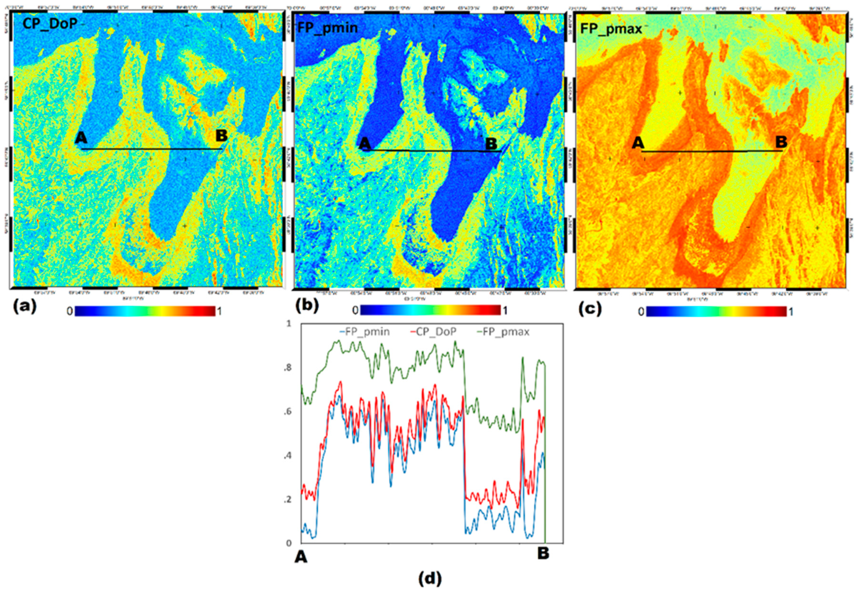
Figure 6 shows visual colour representations illustrating the difference between CP degree of polarization, CP_DoP, the FP Touzi extremas pmin (FP_pmin) and theFP_pmax. In this figure, CP_DoP displays similar behaviour to FP_pmin, with low values over water and vegetated areas and relatively high values over non-vegetated land (bare ground, exposed rocks, and intertidal zones). It was reported previously that the CP_DoP holds a significant edge in detection performance of ships and oil-spills when compared to conventional dual-pol modes (HH-HV) [39]. However, in this study, the contrast is more significant in FP_pmin than the CP_DoP. A slight increase in confusion between these classes is shown in the FP_pmax. This parameter can be used as a complementary source of information (to pmin) for more enhanced contrast, as shown in ship detection [34]. Figure 6d displays the cross profile along the AB transect of the three parameters shown in Figure 6a–c. The profile confirms the colour presentation of the three parameters with a high contrast obtained with FP_pmin and CP_DoP, particularly between the two plateaus of land and water. All three parameters show little contrast between the intertidal zone and upland area, represented with a slight depression in the upper plateau (upland). This suggests that these parameters hold a promising potential to discriminate the intertidal zone.
For quantitative analysis, the contrast between the six classes obtained using the same three parameters is presented in Figure 7a. In addition, polarimetric decomposition using FD is presented in (b) and CP m-delta decomposition parameters are presented in (c). As seen in Figure 7, water surface can be identified most reliably in almost all generated parameters, and the bare ground/dry soil and dry soil/wet soil are the least separable. The DoP extrema pmin shows strong separability capabilities between all classes. In fact, pmin outperforms all the other parameters, followed by volume and surface scattering components of the FD decomposition, pmax, and the surface component of m-delta. For the FD decomposition, vegetation and exposed rocks are dominated by volume scattering whereas double bounce scattering mechanisms are most prevalent in dry soil. In m-delta, the exposed rock class is better discriminated compared to its equivalent in the FD decomposition due to the phase difference. Surface and volume scattering of FD decomposition show similar contrast between intertidal classes. This suggests the presence of sparse vegetation, gravel, or a combination of the two.
4.2. Classification
Table 2 provides the summary of accuracies for various classifiers’ inputs based on RADARSAT-2 and RCM simulated scenarios using the RF algorithm. Figure 8 and Figure 9 present various land cover maps based on listed combinations. The classification results derived from dual scenarios are presented in Figure 8 and Table 2. As expected, the dual conventional co-pol and cross-pol (HH-HV) show better classification results with an overall accuracy of 64.4% followed by RR-RL (61.1%), RH-RL (60.67%), and finally, HH-VV (59.17%). Based on Figure 8 and Table 2, the HH-HV classification map looks similar to the map produced with RR-RL, with high producer’s and user’s accuracies for water exceeding 90% and lower producer’s accuracies for the exposed rocks class of 20.46% (producer’s) and 23.08% (user’s). Both RR-RL and RH-RV exhibit the same behaviour when extracting the vegetation class, as shown in Figure 8. For the bare ground class, all dual scenarios generated producer’s and user’s accuracies exceeding 50%. In intertidal areas, RR-RL and RH-RV produced similar results with the highest success of classification with 55.3% (producer’s) for wet soil. For the dry sand, however, the accuracy is much lower with values ranging between 17% and 34%. Examining Figure 6, one can notice the high confusion between the wet and dry sand classes. Overall, classification accuracies obtained with dual combinations (both conventional and hybrid) show a relative limitation in distinguishing intertidal classes. Using a combination of these parameters along with other types of data such as optical imagery as suggested in other studies [30,31] may increase the overall accuracy results.
Examples of classification results of polarimetric parameters are also shown in Table 2 and Figure 9. Figure 9 presents a comparison between RF classification outputs of FP FD parameters, Touzi discriminators (pmin, pmax, R0max), and CP m-delta parameters. Compared to dual combinations, these classification results show relative improvement with an overall accuracy ranging between 61% and 71%, as shown in Table 2. These results are expected, as the polarimetric parameters (information) tend to provide a better description of geophysical properties of the surface and can therefore account for roughness, biomass, and soil moisture variables.
Among the three classification maps presented in Figure 9, it can be noted that DoP Touzi discriminators have the best visual discrimination ability, followed by FD and the Raney m-delta. Land classes (exposed rocks, vegetation, and bare ground) appear in more defined clusters and are less noisy in Touzi discriminators than in all other decompositions and are closer to the true colour RGB presentation of Sentinel-2 (Figure 2c). Table 2 confirms these results in terms of overall accuracy values. Based on producer’s and user’s accuracies, water emerges as the best contrasted class, exceeding 95% for all parameters.
For the FD results, the lowest accuracy is observed in the exposed rocks class (36.8%) followed by the relatively better results in the bare ground class (~57%). The CP m-delta produced the best user’s accuracy for the exposed rocks (50%), outperforming all other parameters. For intertidal classes, the FD based results show producer’s accuracies of 41% and 42.7% for dry and wet soil classes, respectively. As for Touzi discriminators, the dry soil produces an accuracy of 59% and presents similar results to FD for the wet soil class. For the CP m-delta parameters, wet soil produces an accuracy of 55%, outperforming all the FP results. However, for the dry soil class, the decomposition is the least accurate, with a producer’s accuracy of 28.8%. This can be attributed to two factors. The first is related to the difference of processing of the simulated data compared to RADARSAT-2 imagery, since the RCM CP simulated data was processed with medium resolution as suggested in [36]. Second, the dry soil representing sand bars covers a few clusters of pixels that are not well extracted using a larger window of processing. This confirms that the CP dual polarization results produced slightly less accurate results compared to the conventional dual-pol. Bare ground displayed better discrimination with a value exceeding 53% with m-delta decomposition. For the vegetation class, the Touzi discriminators performed well with a producer’s accuracy of 64%, followed by FD (47.3%), and finally, CP m-delta at 20.2%. Furthermore, an investigation into the potential of other CP parameters including the degree of depolarization (DoD=1−DoP), correlation coefficient, circular polarization ratio, and the conformity coefficient was performed, and the results were added to Table 2. These parameters tend to be less accurate when used separately with an overall accuracy of less than 48%. With exception to the water class, all other classes have low contrast. The use of these parameters must be combined with other sources of information to achieve acceptable results.
Mapping intertidal zones can prove to be complex and challenging, as these areas are subject to continuous changes under the influence of arctic dynamic environmental processes. In summary, the results obtained in this study suggest that the use of a single dual polarization or polarimetric decomposition as a sole source of information to feed the classification process can provide encouraging results. Previous studies [32,33] suggested that the classification can be further enhanced when combined with optical data as tested in a wetland environment. In the case of intertidal zones, analysis is quite challenging as it is difficult to match EO satellite acquisition cycles and a specific tidal stage to generate meaningful information. As expected, the results show that fully polarimetric parameters provide the best accuracy due to their high sensitivity to different types of surfaces, whereas the classification using simulated CP parameters appears to be slightly less accurate. The results show (except for the water class which has been well discriminated in all considered cases) that all classes produce high to higher backscattering values (more than -18dB). The results obtained from the CP m-delta are reasonable when considering the complexity of the environment. The large swath of the compact polarization can factor into the relatively small decrease of classification accuracy when compared to FP results, and could potentially be used for large scale mapping and monitoring purposes.
The obtained results are limited to the study site and therefore the approach should be tested on intertidal zones in different environments to examine the validity and reliability of the methodology. However, most arctic or subarctic intertidal zones are characterized by numerous boulders mixed with muddy to sandy materials [67]. This similar environmental setting to our study area can occur in the large macrotidal coastal stretch along Ungava Bay, suggesting the possibility of getting similar results when applying our approach to these areas. Other intertidal environments, characterized by significant presence of other features such as mangroves and sea grass, might be a challenge which may require an enhancement of the developed methodology.
5. Conclusions
In this study, we investigated the potential of the Canadian RCM mission for mapping intertidal areas. The classification analyses of simulated CP parameters were presented and compared to FP polarimetric information. The potential of both CP and FP for intertidal zone classification has been demonstrated. Results can be enhanced when complemented with conventional dual-pol data, or combined with digital elevation models and optical imagery. As expected, Touzi discriminators (pmin, pmax, R0max) showed the best overall accuracy followed by the FD approach. However, current FP missions are limited when used operationally in mapping large areas. CP is the best suited option for operational use. CP m-delta showed encouraging results and was comparable to well-known FP polarimetric decompositions. In the case of RCM, these results can be considered promising when we highlight the added advantage of a larger swath in an operational mapping context. Furthermore, thanks to its rapid revisit time, the RCM constellation will prove to be an effective monitoring tool for characterizing the changes in coastal areas, particularly in the intertidal zones of northern Canada where the impact of climate change is increasingly apparent.
Author Contributions
Conceptualization, K.O., R.C. and R.T.; methodology, K.O.; validation, K.O., R.T. and R.C.; formal analysis, K.O; investigation, K.O., R.T. and R.C.; writing—original draft preparation, K.O.; writing—review and editing, K.O., R.T., R.C. and M.S. All authors have read and agreed to the published version of the manuscript.
Funding
This research received no external funding.
Acknowledgments
The authors would like to thank the Canadian Space Agency (CSA) for funding this work through the Data Utilization and Application Plan project (DUAP). We thank Paul Wilson and Francis Canisius from NRCan and Adam Jirovec for reviewing the manuscript. We also thank the anonymous reviewers for providing valuable comments.
Conflicts of Interest
The authors declare no conflict of interest.
References
- Airoldi, L.; Beck, M.W. Loss, Status and Trends for Coastal Marine Habitats of Europe. Oceanogr. Mar. Biol. 2007, 45, 345–405. [Google Scholar] [CrossRef]
- Chen, Y.; Dong, J.; Xiao, X.; Zhang, M.; Tian, B.; Zhou, Y.; Li, B.; Ma, Z. Land claim and loss of tidal flats in the Yangtze estuary. Sci. Rep. 2016, 6, 24018. [Google Scholar] [CrossRef] [PubMed]
- Murray, R.S.; Clemens, S.R.; Phinn, H.P.; Possingham, R.A. Fuller Tracking the rapid loss of tidal wetlands in the Yellow Sea Front. Ecol. Environ. 2014, 12, 267–272. [Google Scholar] [CrossRef] [Green Version]
- Short, A.D. Handbook of Beach and Shoreface Morphodynamics; John Wiley and Sons: Chichester, UK, 2004. [Google Scholar]
- Collin, A.; Long, B.; Archambault, P. Merging land-marine realms: Spatial patterns of seamless coastal habitats using a multispectral LiDAR. Remote Sens. Environ. 2012, 123, 390–399. [Google Scholar] [CrossRef]
- Ryu, J.H.; Kim, C.H.; Lee, Y.K.; Won, J.S.; Chun, S.S.; Lee, S. Detecting the intertidal morphologic change using satellite data. Estuar. Coast. Shelf Sci. 2008, 78, 623–632. [Google Scholar] [CrossRef]
- Mason, D.C.; Scott, T.R.; Dance, S.L. Remote sensing of intertidal morphological change in Morecambe Bay, U.K., between 1991 and 2007. Estuar. Coast. Shelf Sci. 2010, 87, 487–496. [Google Scholar] [CrossRef] [Green Version]
- Olliver, E.A.; Edmonds, D.A. Defining the ecogeomorphic succession of land building for freshwater, intertidal wetlands in Wax Lake Delta, Louisiana. Estuar. Coast. Shelf Sci. 2017, 196, 45–57. [Google Scholar] [CrossRef]
- Sagar, S.; Roberts, D.; Bala, B.; Lymburner, L. Extracting the intertidal extent and topography of the Australian coastline from a 28 year time series of Landsat observations. Remote Sens. Environ. 2017, 195, 153–169. [Google Scholar] [CrossRef]
- Ryu, J.H.; Na, Y.H.; Won, J.S.; Doerffer, R. A critical grain size for Landsat ETM+ investigations into intertidal sediments: A case study of the Gomso intertidal flats, Korea. Estuar. Coast. Shelf Sci. 2004, 60, 491–502. [Google Scholar] [CrossRef]
- Murray, N.; Phinn, S.; Clemens, R.; Roelfsema, C.; Fuller, R. Continental scale mapping of tidal flats across East Asia using the Landsat archive. Remote Sens. 2012, 4, 3417–3426. [Google Scholar] [CrossRef] [Green Version]
- Brockmann, C.; Stelzer, K. Optical remote sensing of intertidal flats. In Remote Sensing of the European Seas; Barale, V., Gade, M., Eds.; Springer: Dordrecht, The Netherlands, 2008; pp. 117–128. [Google Scholar] [CrossRef]
- Gade, M.; Alpers, W.; Melsheimer, C.; Tanck, G. Classification of sediments on exposed tidal flats in the German Bight using multi-frequency radar data. Remote Sens. Environ. 2008, 112, 1603–1613. [Google Scholar] [CrossRef]
- Choe, B.-H.; Kim, D.-J.; Hwang, J.-H.; Oh, Y.; Moon, W. Detection of oyster habitat in tidal flats using multi-frequency polarimetric SAR data. Estuar. Coast. Shelf Sci. 2012, 97, 28–37. [Google Scholar] [CrossRef]
- Park, S.-E.; Moon, W.M.; Kim, D.-J. Estimation of surface roughness parameter in intertidal mudflat using airborne polarimetric SAR data. IEEE Trans. Geosci. Remote Sens. 2009, 47, 1022–1031. [Google Scholar] [CrossRef]
- Souza-Filho, P.W.M.; Paradella, W.R.; Rodrigues, S.W.P.; Costa, F.R.; Mura, J.C.; Gonçalves, F.D. Discrimination of coastal wetland environments in the Amazon region based on multi-polarized L-band airborne synthetic aperture radar imagery. Estuar. Coast. Shelf Sci. 2012, 95, 88–98. [Google Scholar] [CrossRef]
- Lee, Y.-K.; Park, J.-W.; Choi, J.-K.; Oh, Y.; Won, J.-S. Potential uses of TerraSAR-X for mapping herbaceous halophytes over salt marsh and tidal flats. Estuar. Coast. Shelf Sci. 2012, 115, 366–376. [Google Scholar] [CrossRef]
- Geng, X.M.; Li, X.M.; Velotto, D.; Chen, K.S. Study of the polarimetric characteristics of mud flats in an intertidal zone using C–and X–band spaceborne SAR data. Remote Sens Environ. 2016, 176, 56–68. [Google Scholar] [CrossRef]
- Gade, M.; Wang, W.; Kemme, L. On the imaging of exposed intertidal flats by single- and dual-co-polarization Synthetic Aperture Radar. Remote Sens. Environ. 2018, 205, 315–328. [Google Scholar] [CrossRef]
- Boerner, W.M.; Mott, H.; Luneburg, E.; Livigstone, C.; Brisco, B.; Brown, R.J.; Paterson, J.S. Polarimetry in radar remote sensing: Basic and applied concepts in “Principles and Applications of Imaging Radar”. In Manual of Remote Sensing, 3rd ed.; Ryerson, R.A., Ed.; John Wiley & Sons: Hoboken, NJ, USA, 1998; Volume 2, pp. 271–358. [Google Scholar]
- Touzi, R.; Gosselin, G.; Brook, R. Polarimetric L-band SAR for peatland mapping and monitoring. In ESA Book on Principles and Applications of Pol-InSAR; Springer: Berlin/Heidelberg, Germany, 2020. [Google Scholar]
- Lee, J.-S.; Pottier, E. Polarimetric Radar Imaging: From Basics to Applications; CRC Press: Boca Raton, FA, USA, 2009. [Google Scholar]
- Banks, S.N.; King, D.J.; Merzouki, A.; Duffe, J. Characterizing scattering behaviour and assessing potential for classification of arctic shore and near-shore land covers with fine quad-pol RADARSAT-2 data. Can. J. Remote Sens. 2014, 40, 291–314. [Google Scholar] [CrossRef]
- Freeman, A.; Durden, S. A three-component scattering model for polarimetric SAR data. IEEE Trans Geosci. Remote Sens. 1998, 36, 963–973. [Google Scholar] [CrossRef] [Green Version]
- Cloude, S.R.; Pottier, E. An Entropy Based Classification Scheme for Land Applications of Polarimetric SAR. IEEE Trans. Geosci. Remote Sens. 1997, 35, 68–78. [Google Scholar] [CrossRef]
- Wang, W.; Yang, X.; Li, X. A Fully Polarimetric SAR Imagery Classification Scheme for Mud and Sand Flats in Intertidal Zones. IEEE Trans. Geosci. Remote Sens. 2017, 55, 1734–1742. [Google Scholar] [CrossRef]
- Singhroy, V.; Charbonneau, F. RADARSAT: Science and applications. Phys. Can. 2014, 70, 212–217. [Google Scholar]
- Thompson, A. Overview of the RADARSAT constellation mission. Can. J. Remote Sens. 2015, 41, 401–407. [Google Scholar] [CrossRef]
- Raney, R.K. Hybrid-polarity SAR architecture. IEEE Trans. Geosci. Remote Sens. 2007, 45, 3397–3404. [Google Scholar] [CrossRef] [Green Version]
- Dabboor, M.; Geldsetzer, T. Towards sea ice classification using simulated RADARSAT Constellation Mission compact polarimetric SAR imagery. Remote Sens Environ. 2014, 140, 189–195. [Google Scholar] [CrossRef]
- Geldsetzer, T.; Charbonneau, F.; Arkett, M.; Zagon, T. Ocean Wind Study Using Simulated RCM Compact-Polarimetry SAR. Can. J. Remote Sens. 2015, 41, 418–430. [Google Scholar] [CrossRef]
- White, L.; Millard, K.; Banks, S.; Richardson, M.; Pasher, J.; Duffe, J. Moving to the RADARSAT Constellation Mission: Comparing Synthesized Compact Polarimetry and Dual Polarimetry Data with Fully Polarimetric RADARSAT-2 Data for Image Classification of Peatlands. Remote Sens. 2017, 9, 573. [Google Scholar] [CrossRef] [Green Version]
- Banks, S.; Millard, K.; Behnamian, A.; White, L.; Ullmann, T.; Charbonneau, F.; Chen, Z.; Wang, H.; Pasher, J.; Duffe, J. Contributions of Actual and Simulated Satellite SAR Data for Substrate Type Differentiation and Shoreline Mapping in the Canadian Arctic. Remote Sens. 2017, 9, 1206. [Google Scholar] [CrossRef] [Green Version]
- Touzi, R.; Vachon, P.W. Vachon PWRCM polarimetric SAR for enhanced ship detection classification. Can. J. Remote Sens. 2015, 41, 473–484. [Google Scholar] [CrossRef]
- Raney, R.K. Hybrid Dual-Polarization Synthetic Aperture Radar. Remote Sens. 2019, 11, 1521. [Google Scholar] [CrossRef] [Green Version]
- Charbonneau, F.; Brisco, B.; Raney, K.; McNairn, H.; Liu, C.; Vachon, P.; Shang, J.; De Abreu, R.; Champagne, C.; Merzouki, A.; et al. Compact polarimetry overview and applications assessment. Can. J. Remote Sens. 2010, 36 (Suppl. 2), S298–S315. [Google Scholar] [CrossRef]
- Touzi, R. Hybrid Versus Matched Antenna for Dual- and Fully Polarimetric SAR; PolinSAR’13; Frascatti: Rome, Italy, 2013. [Google Scholar]
- Touzi, R.; Hurley, J.; Vachon, P. Optimization of the Degree of Polarization for Enhanced Ship Detection Using Polarimetric RADARSAT-2. IEEE Trans. Geosci. Remote Sens. 2015, 53, 5403–5424. [Google Scholar] [CrossRef]
- Shirvany, R.; Chabert, M.; Tourneret, J.-Y. Ship and oil-spill detection using the degree of polarization in linear and hybrid/compact dual-pol SAR. IEEE J. Sel. Top. Appl. Earth Obs. Remote Sens. 2012, 5, 885–892. [Google Scholar] [CrossRef] [Green Version]
- Marino, A. A notch filter for ship detection with polarimetric SAR images. IEEE J. Sel. Top. Appl. Earth Obs. Remote Sens. 2013, 6, 1219–1232. [Google Scholar] [CrossRef] [Green Version]
- Souyris, J.-C.; Imbo, P.; Fjortoft, R.; Mingot, S.; Lee, J.-S. Compact polarimetry based on symmetry properties of geophysical media: The pi/4 mode. IEEE Trans. Geosci. Remote Sens. 2005, 43, 634–646. [Google Scholar] [CrossRef]
- Raney, R.K.; Cahill, J.T.S.; Patterson, G.W.; Bussey, D.B.J. The M-Chi Decomposition of Hybrid Dual-Polarimetric Radar Data with Application to Lunar Craters. J. Geophys. Res. Planets 2012, 117. [Google Scholar] [CrossRef]
- Xu, L.; Zhang, H.; Wang, C.; Zhang, B.; Tian, S. Compact polarimetric SAR ship detection with m- decomposition using visual attention model. Remote Sens. 2016, 8, 751. [Google Scholar] [CrossRef] [Green Version]
- Yin, J.; Yang, J. Ship detection by using the M-Chi and M-Delta decompositions. In Proceedings of the IEEE International Geoscience and Remote Sensing Symposium (IGARSS), Quebec, QC, Canada, 13–18 July 2014. [Google Scholar] [CrossRef]
- Collins, M.J.; Denbina, M.; Atteia, G. On the reconstruction of quad-pol SAR data from compact polarimetry data for ocean target detection. IEEE Trans. Geosci. Remote Sens. 2013, 51, 591–600. [Google Scholar] [CrossRef]
- Li, H.Y.; Perrie, W.; He, Y.J.; Lehner, S.; Brusch, S. Target detection on the ocean with the relative phase of compact polarimetry SAR. IEEE Trans. Geosci. Remote Sens. 2013, 51, 3299–3305. [Google Scholar] [CrossRef]
- Lopez-Sanchez, J.M.; Vicente-Guijalba, F.; Ballester-Berman, J.D.; Cloude, S.R. Polarimetric Response of Rice Fields at C-Band: Analysis and Phenology Retrieval. IEEE Trans. Geosci. Remote Sens. 2014, 52, 2977–2993. [Google Scholar] [CrossRef] [Green Version]
- Yang, Z.; Li, K.; Liu, L.; Shao, Y.; Brisco, B.; Li, W.G. Rice growth monitoring using simulated compact polarimetric C band SAR. Radio Sci. 2014, 49, 1300–1315. [Google Scholar] [CrossRef]
- Singha, S.; Ressel, R. Arctic sea ice characterization using RISAT-1 compact-pol SAR imagery and feature evaluation: A case study over North-East Greenland. IEEE J. Sel. Top. Appl. Earth Obs. Remote Sens. 2017, 10, 3504–3514. [Google Scholar] [CrossRef] [Green Version]
- Espeseth, M.; Brekke, C.; Johansson, A. Assessment of RISAT-1 and RADARSAT-2 for Sea Ice Observations from a Hybrid-Polarity Perspective. Remote Sens. 2017, 9, 1088. [Google Scholar] [CrossRef] [Green Version]
- Li, H.Y.; Perrie, W. Sea Ice Characterization and Classification Using Hybrid Polarimetry SAR. IEEE J. Sel. Topics Appl. Earth Obs. Remote Sens. 2016, 9, 4998–5010. [Google Scholar] [CrossRef]
- Dabboor, M.; Iris, S.; Singhroy, V. The RADARSAT Constellation Mission in Support of Environmental Applications. Proceedings 2018, 2, 323. [Google Scholar] [CrossRef] [Green Version]
- Chenier, R.; Omari, K.; Ahola, R.; Sagram, M. Charting Dynamic Areas in the Mackenzie River with RADARSAT-2, Simulated RADARSAT Constellation Mission and Optical Remote Sensing Data. Remote Sens. 2019, 11, 1523. [Google Scholar] [CrossRef] [Green Version]
- Sun, T.; Zhang, G.; Perrie, W.; Zhang, B.; Guan, C.; Khurshid, S.; Warner, K.; Sun, J. Ocean Wind Retrieval Models for RADARSAT Constellation Mission Compact Polarimetry SAR. Remote Sens. 2018, 10, 1938. [Google Scholar] [CrossRef] [Green Version]
- Yin, J.; Yang, J.; Zhou, Z.-S.; Song, J. The extended bragg scattering model-based method for ship and oil-spill observation using compact polarimetric SAR. IEEE J. Sel. Topics Appl. Earth Observ. Remote Sens. 2014, 8, 3760–3772. [Google Scholar] [CrossRef]
- Sivasankar, T.; Srivastava, H.S.; Sharma, P.K.; Kumar, D.; Patel, P. Study of hybrid polarimetric parameters generated from risat-1 SAR data for various land cover targets. Int. J. Adv. Remote Sens. Gis Grogr. 2015, 3, 32–42. [Google Scholar]
- Allard, M.; Calmels, F.; Fortier, D.; Laurent, C.; L’Hérault, E.; Vinet, F. Cartographie des conditions de pergélisol dans les communautés du Nunavik en vue de l’adaptation au réchauffement climatique. In Réalisé Pour le Compte d’Ouranos, Ressources Naturelles Canada; Centre D’études Nordiques, Université Laval: Québec City, QC, Canada, 2007; 42p, Available online: https://www.ouranos.ca/publication-scientifique/RapportAllard2007_FR.pdf (accessed on 11 January 2020).
- Vinet, F. Géomorphologie, Stratigraphie et Évolution du Niveau Marin Holocène D’une Vallée Soumise à des Conditions Macrotidales en Régression Forcée, Région de Tasiujaq, Nunavik. Master’s Thesis, Université Laval, Département de Géographie, Québec City, QC, Canada, 2008. Unpublished. Available online: http://hdl.handle.net/20.500.11794/19578 (accessed on 12 January 2020).
- Arbic, B.K.; St-Laurent, P.; Sutherland, G.; Garrett, C. On the resonance and influence of the tides in Ungava Bay and HudsonStrait. Geophys. Res. Lett. 2007, 34. [Google Scholar] [CrossRef] [Green Version]
- Dignard, N.; Michaud, A. La Flore Vasculaire de L’aire D’étude du Projet de Parc National de la Baie-Aux-Feuilles, Québec (58°45′N., 69°35′O.); Ministère des Ressources Naturelles, Direction de la Recherche Forestière: Québec City, QC, Canada, 2013; 218p. Available online: https://mffp.gouv.qc.ca/nos-publications/flore-vasculaire-baie-aux-feuilles/ (accessed on 12 January 2020).
- Touzi, R.; Charbonneau, F.J. PWS: A friendly and effective tool for polarimetric image analysis. Can. J. Remote Sens. 2004, 30, 566–571. [Google Scholar] [CrossRef]
- Breiman, L. Random Forests. Mach. Learn. 2001, 45, 5–32. [Google Scholar] [CrossRef] [Green Version]
- Lawrence, R.L.; Wood, S.D.; Sheley, R.L. Mapping invasive plants using hyperspectral imagery and Breiman Cutler classifications (random forest). Remote Sens. Environ. 2006, 100, 356–362. [Google Scholar] [CrossRef]
- Rodriguez-Galiano, V.F.; Ghimire, B.; Rogan, J.; Chica-Olmo, M.; Rigol-Sanchez, J.P. An assessment of the effectiveness of a random forest classifier for land-cover classification. ISPRS J. Photogramm. Remote Sens. 2012, 67, 93–104. [Google Scholar] [CrossRef]
- VanBeijma, S.; Comber, A.; Lamb, A. Random forest classification of salt marsh vegetation habitats using quad-polarimetric airborne SAR, elevation and optical RS data. Remote Sens. Environ. 2014, 149, 118–129. [Google Scholar] [CrossRef]
- Corcoran, J.M.; Knight, J.F.; Gallant, A.L. Influence of Multi-Source and Multi-Temporal Remotely Sensed and Ancillary Data on the Accuracy of Random Forest Classification of Wetlands in Northern Minnesota. Remote Sens. 2013, 5, 3212–3238. [Google Scholar] [CrossRef] [Green Version]
- Archer, A.W. World’s highest tides: Hypertidal coastal systems in North America, South America, and Europe. Sediment. Geol. 2013, 284–285, 1–25. [Google Scholar] [CrossRef]
Figure 1.
RADARSAT-2 RGB presentations (Red: HH, Green: HV, and Blue: VV) of the study area acquired on September 6, 2016, corresponding to low tide. Yellow squares and rectangles show air photo sites within the area. RADARSAT-2 Data and Products© MacDonald, Dettwiler and Associates Ltd. (2016)—All Rights Reserved. RADARSAT is an official mark of the Canadian Space Agency.

Figure 2.
RADARSAT-2 RGB presentations (Red: HH, Green: HV, and Blue: VV) of the study area acquired on (a) the 6 September 2016, corresponding to low tide and (b) 13 August 2016, corresponding to low tide. (c) is an RGB of Sentinel-2 acquired 28 August 2018. RADARSAT-2 Data and Products© MacDonald, Dettwiler and Associates Ltd. (2016)—All Rights Reserved. RADARSAT is an official mark of the Canadian Space Agency.

Figure 3.
Example of classes present at the study area. (a) is an air-photo over a part of the intertidal zone of the study area acquired on August 23, 2015, and (b) is an RGB colour composite of Worldview-2 data acquired on 21 August 2014. ©2014, Digital Globe.
Figure 3.
Example of classes present at the study area. (a) is an air-photo over a part of the intertidal zone of the study area acquired on August 23, 2015, and (b) is an RGB colour composite of Worldview-2 data acquired on 21 August 2014. ©2014, Digital Globe.

Figure 4.
RADARSAT-2 scene over the study area. (a) fully polarimetric (FP) polarimetric Freeman–Durden decomposition (red: double bounce, green: volume scattering and blue: surface scattering), (b) RGB composite of Touzi extrema parameters (red: pmin, green: Pmax, and blue: R0max) of FP polarimetric data and (c) m-delta compact polarimetric (CP) decomposition of Circular-Transmit-Linear-Receive (CTLR) simulated (red: even bounce, green: volume, and blue: odd bounce).

Figure 5.
Illustration of the distribution of both training (yellow) and validation (red) samples across the study area.
Figure 5.
Illustration of the distribution of both training (yellow) and validation (red) samples across the study area.

Figure 6.
Colour presentation of (a) the CP degree of polarization CP_DoP, the FP Touzi extremas FP_pmin (b), and FP_pmax (c) of the study area. The graph (d) shows the profile of the three parameters between two points A and B along the line shown in (a–c). The red colour refers to CP_DoP, the blue to FP_min, and green to FP_max.

Figure 7.
Contrast between generated FP and CP parameters for all study area classes based on (a) FP Touzi extremas (FP_pmin FP_pmax) and CP degree of polarization (CP_DoP), (b) Freeman–Durdan (surface, double-bounce, and volume) scattering parameters and (c) CP Raney decomposition (m-delta surface, m-delta double, and m-delta volume).

Figure 8.
Classification maps of dual polarization HH-HV, RH-RV, RR-RL, and HH-VV using a random forest classification approach.
Figure 8.
Classification maps of dual polarization HH-HV, RH-RV, RR-RL, and HH-VV using a random forest classification approach.

Figure 9.
Classification maps of the study area obtained from (a) Freeman–Durden, (b) Touzi discriminators (pmin, pmax, and R0max), and (c) the compact polarimetry m-delta. Maps are generated using a random forest algorithm.
Figure 9.
Classification maps of the study area obtained from (a) Freeman–Durden, (b) Touzi discriminators (pmin, pmax, and R0max), and (c) the compact polarimetry m-delta. Maps are generated using a random forest algorithm.


Table 1.
Contrast between different classes for original and simulated single polarizations in |dB|.
Table 1.
Contrast between different classes for original and simulated single polarizations in |dB|.
| Water | Wet Soil | Dry Soil | Bare Ground | Exposed Rocks | Vegetation | |
|---|---|---|---|---|---|---|
| HH | 29.4 | 15.2 | 12.3 | 12.3 | 2.7 | 10.9 |
| HV | 34.6 | 26.5 | 23.9 | 22.1 | 14.1 | 18.5 |
| VV | 28.1 | 15.2 | 12.5 | 12.7 | 2.9 | 11.3 |
| RH | 23.4 | 14.9 | 10.2 | 12.8 | 5.4 | 12.1 |
| RV | 23.2 | 14.9 | 11.2 | 13.3 | 6.3 | 12.3 |
| RR | 23.5 | 18.2 | 14.2 | 16.6 | 10.7 | 13.1 |
| RL | 23.1 | 13 | 8.8 | 11.1 | 3.6 | 11.4 |
Table 2.
Classification accuracies (%) of derived from the polarimetric (Polar) FP and CP, dual (classical and hybrid), and few single CP simulated parameters. FD refers to Freeman–Durden, Cor. coef. refers to correlation coefficient and Cir. pol. Rat. to circular polarization ratio, DoD refers to the degree of polarization, Kappa Coef. refers to Kappa coefficient, and Veg. refers to vegetation.
| Parameters | Producer’s Accuracy (%) | User’s Accuracy (%) | Overall Accuracy (%) | Kappa Coef. | |||||||||||
|---|---|---|---|---|---|---|---|---|---|---|---|---|---|---|---|
| Water | Wet Soil | Dry Soil | Bare Ground | Veg. | Exposed Rocks | Water | Wet Soil | Dry Soil | Bare Ground | Veg. | Exposed Rocks | ||||
| Polar | FD | 97.31 | 42.72 | 41.01 | 57.19 | 47.29 | 36.74 | 93.53 | 65.67 | 37.01 | 66.09 | 50.41 | 17.14 | 67.08 | 0.564 |
| Touzi * | 94.84 | 42.72 | 58.99 | 72.75 | 64.00 | 42.86 | 87.50 | 94.44 | 76.92 | 20.00 | 77.78 | 10.00 | 71.08 | 0.611 | |
| m-delta | 97.31 | 55.34 | 28.78 | 53.29 | 20.16 | 20.00 | 93.94 | 31.32 | 27.40 | 54.27 | 41.94 | 50.00 | 62.08 | 0.493 | |
| Dual | HH/HV | 94.85 | 49.33 | 33.91 | 55.32 | 46.09 | 20.46 | 95.63 | 50.69 | 35.14 | 61.18 | 33.97 | 23.08 | 64.40 | 0.529 |
| RH/RV | 97.31 | 55.34 | 17.27 | 51.20 | 11.63 | 18.37 | 93.53 | 24.89 | 20.51 | 52.94 | 81.00 | 30.61 | 59.17 | 0.455 | |
| RR/RL | 97.31 | 55.34 | 20.86 | 53.29 | 21.71 | 14.29 | 93.53 | 28.64 | 24.58 | 53.45 | 40.00 | 43.75 | 61.08 | 0.479 | |
| HH/VV | 94.17 | 42.72 | 25.90 | 57.49 | 20.16 | 20.41 | 95.24 | 33.85 | 30.25 | 55.01 | 21.85 | 23.81 | 60.67 | 0.475 | |
| Single | DoD | 94.62 | 0.00 | 13.67 | 25.15 | 16.28 | 38.78 | 71.04 | 0.00 | 19.19 | 48.84 | 17.50 | 8.84 | 47.08 | 0.293 |
| Cor. coef. | 92.83 | 28.16 | 1.44 | 0.00 | 14.73 | 42.86 | 69.58 | 13.49 | 25.00 | 0.00 | 20.88 | 7.22 | 40.42 | 0.238 | |
| Cir. pol. rat. | 86.32 | 78.64 | 0.00 | 6.29 | 1.55 | 4.08 | 74.76 | 13.73 | 0.00 | 28.77 | 20.00 | 0.00 | 40.92 | 0.242 | |
| Conformity | 92.38 | 47.57 | 0.00 | 27.27 | 8.00 | 24.49 | 64.58 | 13.39 | 0.00 | 42.27 | 16.67 | 12.37 | 42.83 | 0.238 | |
* Touzi refers to the Touzi discriminators (pmin, pmax and R0max).
© 2020 by the authors. Licensee MDPI, Basel, Switzerland. This article is an open access article distributed under the terms and conditions of the Creative Commons Attribution (CC BY) license (http://creativecommons.org/licenses/by/4.0/).
Share and Cite
MDPI and ACS Style
Omari, K.; Chenier, R.; Touzi, R.; Sagram, M. Investigation of C-Band SAR Polarimetry for Mapping a High-Tidal Coastal Environment in Northern Canada. Remote Sens. 2020, 12, 1941. https://0-doi-org.brum.beds.ac.uk/10.3390/rs12121941
AMA Style
Omari K, Chenier R, Touzi R, Sagram M. Investigation of C-Band SAR Polarimetry for Mapping a High-Tidal Coastal Environment in Northern Canada. Remote Sensing. 2020; 12(12):1941. https://0-doi-org.brum.beds.ac.uk/10.3390/rs12121941
Chicago/Turabian StyleOmari, Khalid, René Chenier, Ridha Touzi, and Mesha Sagram. 2020. "Investigation of C-Band SAR Polarimetry for Mapping a High-Tidal Coastal Environment in Northern Canada" Remote Sensing 12, no. 12: 1941. https://0-doi-org.brum.beds.ac.uk/10.3390/rs12121941
Note that from the first issue of 2016, this journal uses article numbers instead of page numbers. See further details here.