Spatiotemporal Derivation of Intermittent Ponding in a Maize–Soybean Landscape from Planet Labs CubeSat Images

Abstract

Climate change is increasing the frequency and intensity of heavy precipitation in the US Midwest, overwhelming existing tile drainage, and resulting in temporary soil ponding across the landscape. However, lack of direct observations of the dynamics of temporal soil ponding limits our understanding of its impacts on crop growth and biogeochemical cycling. Satellite remote sensing offers a unique opportunity to observe and analyze this dynamic phenomenon at the landscape scale. Here we analyzed a series of red–green–blue (RGB) and near infrared (NIR) remote sensing images from the Planet Labs CubeSat constellation following a period of heavy precipitation in May 2017 to determine the spatiotemporal characteristics of ponding events in the maize–soybean cropland of Champaign County, Illinois USA. We trained Random Forest algorithms for near-daily images to create binary classifications of surface water versus none, which achieved kappa values around 0.9. We then analyzed the morphology of classification results for connected pixels across space and time and found that 2.5% (5180 ha) of this cropland was classified as water surface at some point during this period. The frequency distribution of areal ponding extent exhibited a log–log relationship; the mean and median areas of ponds were 1231 m² and 126 m², respectively, with 26.1% of identified ponds being at the minimum threshold area of 45 m², and 2.5% of the ponds having an area greater than 104 m² (1 ha). Ponds lasted for a mean duration of 2.4 ± 1.7 days, and 2.3% of ponds lasted for more than a week. Our results suggest that transient ponding may be significant at the landscape scale and ought to be considered in assessments of crop risk, soil and water conservation, biogeochemistry, and sustainability.

1. Introduction

Recent developments in remote sensing platforms facilitate high spatiotemporal resolution detection and monitoring of potentially important but transient phenomena occurring on the Earth’s surface, filling the gaps where previous platforms have been incapable of providing these data. Greater radiative forcing from greenhouse gases produces higher temperatures, increases evaporation rate, and increases the capacity of the atmosphere to carry water vapor, resulting in an increased number of heavy precipitation events and increased streamflow [1]. In the eastern half of the United States, these extreme events are particularly evident during the spring season [2,3]. This new hydrological regime of intense rainfall events and amplified seasonality is likely to increase the frequency of damaging flood events in the region [4], especially soil ponding. Transient soil ponding, besides being a nuisance to row crop agriculture, may potentially alter the biogeochemical balance of agroecosystems [5,6,7,8]. As the frequency and intensity of precipitation increase in the Corn Belt [9,10,11], ponding frequency and extent are also likely to increase as the climate continues to warm. These ponding events will likely have a greater effect on crop yields and biogeochemical cycles in the maize–bean agroecosystem as they increase in frequency, so detecting and monitoring these events will only become more important. Because ponding occurs repeatedly in the same locations and due to recent advances in precision agriculture [12], these areas may provide opportunities to grow perennial bioenergy crops that are more flood-tolerant than maize and soybean [13] or to develop artificial wetlands [14].

It is not uncommon to observe localized flooding—ponding—in tile-drained fields following heavy precipitation events, either because the drainage tiles are not functioning properly or because the inundation exceeds their capacity to rapidly remove surface water. Temporary ponds are inland surface water bodies that emerge and subside dependent on precipitation, soil, and topography [5]. The combination of typically poorly drained soils and the relatively wet climate of the US Corn Belt requires the installation of subsurface tile drain systems in agricultural fields to grow corn and soybeans [15,16]. Tile drainage helps remove surface water and lowers the water table, resulting in deeper-rooted crop plants that are more resilient to water stress. The Corn Belt states have drained approximately 70% of their pre-nineteenth century wetlands, much of it converted to intensive agriculture nowadays [17]; approximately 37% of total Corn Belt cropland is drained by tile drains or surface drainage [16]. Most of the drainage systems of this region were first installed from 1850 to 1930 with the support of federal and state policies [17]. Tile drains made from perforated plastic pipes, or clay for older installations, are buried 0.6 to 1.2 m deep and 10 to 30 m apart, and discharge into nearby streams or ditches [15]. This underground infrastructure is a critical part of Corn Belt hydrology, but the heterogeneous distribution of soil types, microtopography, and tile drainage challenges the development of comprehensive predictions for how the landscape will respond to climate change.

The general trade-off in remote sensing is between spatial and temporal resolution [18,19], a tradeoff that makes it difficult to use remote sensing to observe small, transient phenomena such as ponding. Platforms such as Landsat and Sentinel-2 have sufficient spatial resolution at 30 m and 10 m, respectively, to detect larger ponds [20,21], but with pass rates exceeding one week for Landsat and 5 days for Sentinel-2, they are unable to monitor the fast-changing dynamics of transient events like soil ponding. MODIS (Moderate Resolution Imaging Spectrometer) and VIIRS (Visible Infrared Imagine Radiometer Suite) have sufficient temporal resolution for daily imaging [22,23], but with their spatial resolutions exceeding 250-m, they can only capture extremely large ponds.

Planet’s large constellation of high spatial resolution cube satellites, PlanetScope, overcomes the challenge of obtaining high spatiotemporal resolution imagery. The PlanetScope platform is a constellation of CubeSats in the 3U form factor (10-cm × 10-cm × 30-cm), with a target constellation size of 130 satellites [24]. PlanetScope is a commercial product that typically requires payment for access but is also available for research and education purposes at no charge through an application process. The full constellation will be capable of daily 3-m resolution red–green–blue near infrared (RGB–NIR) imaging for the entire Earth’s surface, providing unprecedented spatiotemporal resolution and coverage among remote sensing platforms. Thus, the PlanetsScope constellation is capable of overcoming the spatial and temporal resolution trade-off of typical remote sensing platforms, which is essential for this transient ponding detection application.

The objective of this study was to develop a remote sensing method based on Planet CubeSat data to detect ephemeral dynamics of ponding in an agricultural landscape, and to quantify the spatial extent and duration of ponds after a major precipitation event. We automated ponding detection using Random Forest [25], a robust supervised machine learning algorithm. The ability to measure the size and duration of ephemeral ponds with high accuracy will enable monitoring the alterations to surface hydrology and their rapidly shifting dynamics as the climate system changes.

2. Materials and Methods

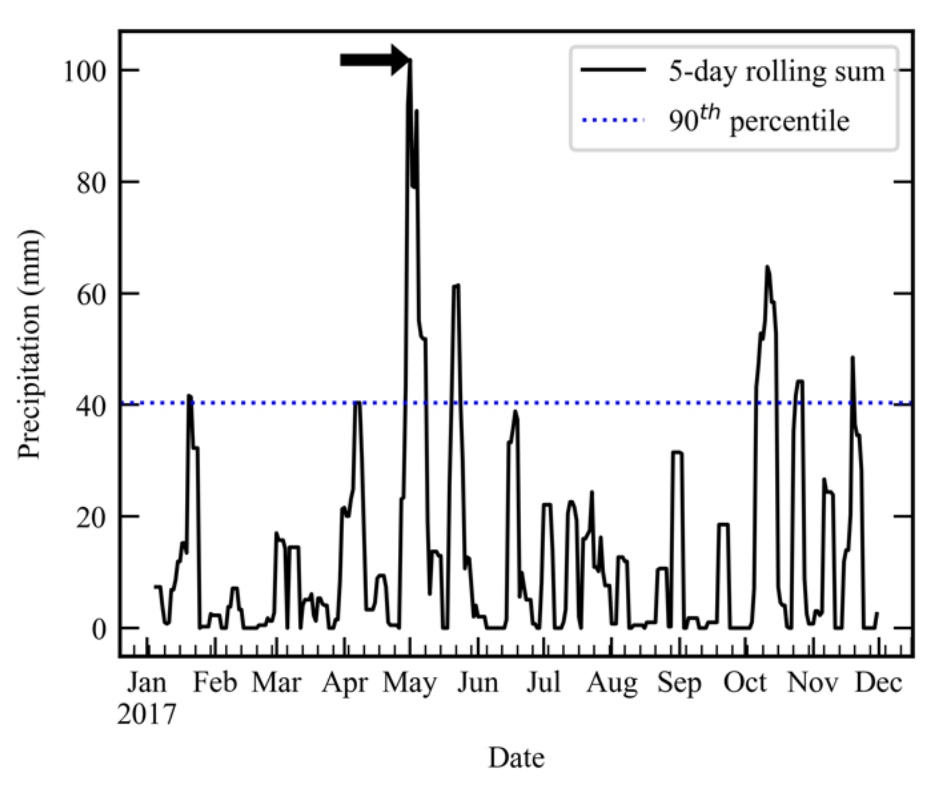
2.1. Identify the Extreme Rainfall Event for Analysis

We analyzed a series of RGB–NIR remote sensing images from the Planet Labs satellite constellation [26] following a period of heavy precipitation in May 2017 to determine the spatiotemporal characteristics of flooding events in the maize–soybean cropland of Champaign County, Illinois. This area is strongly dominated by row crop agriculture featuring an annual rotation of maize and soybean, and is representative of cropping systems in much of the Midwest US. We focused on early spring just prior to crop emergence when the probability of intense precipitation events is greatest and when detecting soil ponding is not obscured by plant cover.

To determine the size and duration of ponding events, we first identified high precipitation periods from the top 90th percentile of five-day rolling sums of daily precipitation for Champaign County in 2017. Precipitation data for Champaign County were obtained from the cli-MATE database [27]. We also constrained the selection to days outside of canopy closure during the maize and bean growing season. For our primary analysis of pond size and duration we selected the weeks following a high precipitation period (125 mm total accumulation/week) ending on 5 May 2017 (Figure 1).

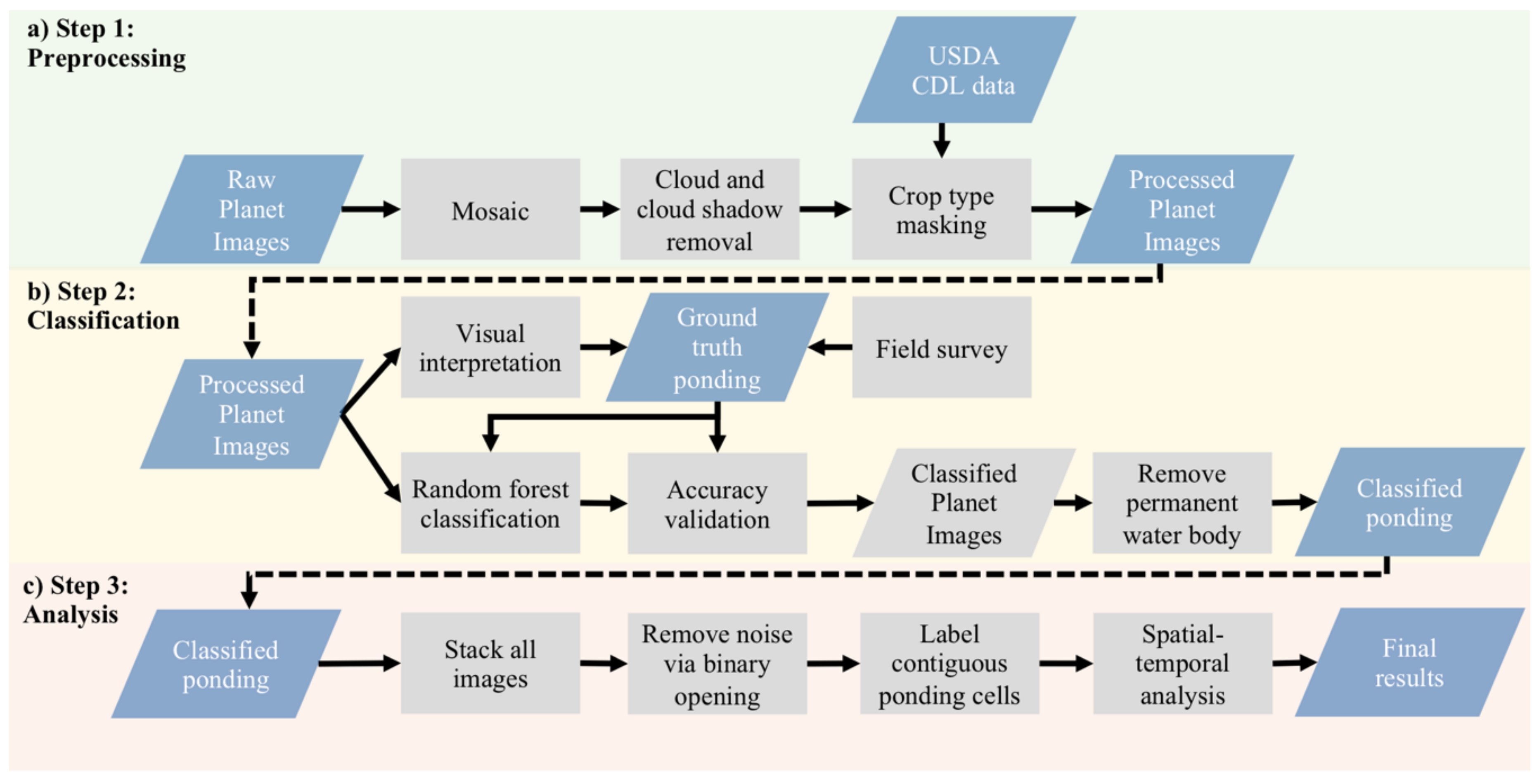
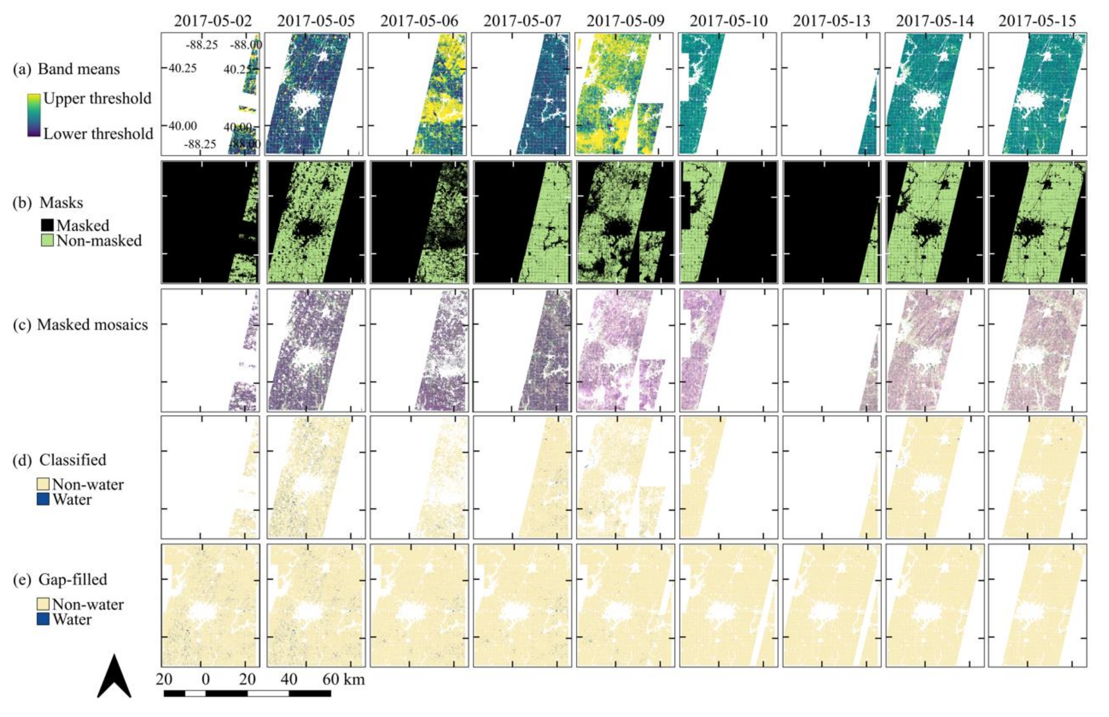
2.2. Preprocessing Planet Images

For each day following this high precipitation period in May 2017, we collected and processed 3-m resolution RGB–NIR imagery of Champaign County from the Planet Labs satellite constellation [26] (Figure 2a). We had 9 days of usable imagery from 3 May 2017 to 15 May 2017, inclusive. We used Google Earth Engine [28] to mosaic the images, mask out obscurations such as clouds and shadows, and ensure alignment between these intermediate raster products (Table S1). We took the mean of the digital number values for all bands at each pixel, which we used to generate masks with simple cut-offs of high and low threshold values (Table S2). We removed digital artifacts around cloud shadows by adding a 150 m buffer around cloud shadows because the classifier detected some of these artifacts as false positives for the water surface. We masked out land cover not classified as maize, soybean, or water according to the 2017 Cropland Data Layer (CDL) [29]. We resampled the raster data and masks on export from Google Earth Engine so that all images completely matched in projection, extent, scale, and alignment of pixels, using the minimal bounding box containing Champaign County to define the origin and dimensions of raster extents. We included permanent water features in training the classifier to provide additional spectral data associated with water, but we later masked out these features before the spatiotemporal analyses.

2.3. Classifying Ponding Areas Using Random Forest

For each mosaicked image we trained Random Forest algorithms separately [25] with surface type-attributed polygons as labeling data to create binary classifications of surface water versus none using the RStoolbox (v. 0.2.6) [30] package in R (v. 3.5.1) (Figure 2b), which is a remote sensing-oriented wrapper for the caret package (v. 6.0.8) [31]. All the ground truth labeling data were generated through visual interpretation of images on each single day. The random forest classifier on a specific day was trained only using the labeling data collected on that day. To validate the surface water classification, mosaicked images were compared to a road survey of ponding. On 5 May 2017, we recorded the GPS locations of ponds visually identified from a road survey during the high precipitation period at the start of May 2017. The survey path length was approximately 33 km in the northwest quadrant of Champaign County, and included 39 recorded points of ponding locations. Water features identified from the road survey were readily distinguishable in the mosaicked rasters through false color imaging using the red, blue, and NIR bands for display, which we used to construct the training data for the classifications.

Using QGIS (v. 3.4.15) [32] we generated ground truth labels through visual interpretation of images on each single day. Two remote sensing experts worked on each image at the same time and doing cross-check with each other. Only those areas identified as ponding by both experts were used as areas of interest to generate labeling data. We randomly generated points in the areas of interest and produced polygons using the points as centroids. For each available day, we repositioned and reshaped the polygons to contain only water or to completely exclude water, and then attributed them with their binary land cover type. We used the classified polygons as the training data for the Random Forest algorithms in a 10-fold cross-validation to predict binary classifications of surface water versus none, reserving 10% of training samples, randomly selected, for each day to independently validate the predictions.

After we generated the classifications, we masked out permanent water features as defined by the CDL. We also compared the classified images with images from a dry period as a negative control to show that long-lasting ponds were not overrepresented by permanent features below the CDL’s detection threshold. To produce the dry period classification, we used the same method as the wet period images but retained “water” land cover types from the CDL. We analyzed each classification result for accuracy primarily by calculating the associated kappa value from the independent validation. Kappa is formally described as:

$$\kappa =\frac{p_0-p_c}{1-p_c}$$

(1)

where p₀ is the overall accuracy, the total proportion of correctly predicted classifications, and p_c is the proportion expected to agree by chance alone [33]. We used a threshold kappa of 0.7; we added more training polygons when a classification fell below the threshold kappa. The 95% confidence intervals (CI) of overall accuracy were estimated using the binomial test. Other performance metrics used in this study include no information rate, sensitivity, and specificity, with their definitions as follows:

$$\mathit{No} \mathit{information} \mathit{rate} = \left({‘\mathit{surface} \mathit{water}’}_{ \mathit{total}}\%,{‘\mathit{not} \mathit{water}’}_{ \mathit{total}}\%\right)$$

(2)

$$\mathit{Sensitivity} = {‘\mathit{surface} \mathit{water}’}_{ \mathit{correctly} \mathit{predicted}} / {‘\mathit{surfacewater}’}_{ \mathit{total}}$$

(3)

$$\mathit{Specificity} = {‘\mathit{not} \mathit{water}’}_{ \mathit{correctly} \mathit{predicted}} / {‘\mathit{not} \mathit{water}’}_{ \mathit{total}}$$

(4)

2.4. Spatiotemporal Analysis of Ponding Dynamics

For the morphological analyses of classified rasters from the multiple days following a heavy precipitation event, we used the multidimensional image processing tools from the Scipy package (v. 1.1.0) in Python (v. 3.7.2) [34] (Figure 2c and Figure 3). We stacked the days together sequentially with time along the z-axis (Figure 3a). We removed noise via binary opening with a 5-cell, 45 m² structuring element; the structuring element was arranged as a central cell with four directly adjacent cells in the x and y dimensions, so all non-contiguous cells smaller than the structuring element were dropped from the morphological analysis (Figure 3b). We gap-filled missing data, whether due to obscurations or unavailable image extent, by duplicating classification data from the next available day (Figure 3c). We labeled spatially and temporally contiguous cells to define features, each of which was labelled sequentially in order of detection along the x, y, and then z axes (Figure 3d). We described feature duration distribution by analyzing how many days each labeled feature lasted, starting on the first day with precipitation below 0.5 cm, 6 May 2017. We used the gap-filled data from 6 May 2017, to determine the areal distribution of ponds by analyzing the areal extent of each labeled feature. All code used for pre-processing and analysis is available at github.com/rfpaul/Flooding_Laszlo.

3. Results

For our independent validation, our kappa values across all analyzed days ranged from 0.823 to 0.9996, suggesting that we had excellent accuracy for the classifiers (

Table 1. Accuracy statistics of classifier per date at the start of May 2017. All data were trained on 10-fold cross-validations benchmarked on kappa values. These statistics are from independent validations performed by reserving 10% of the training polygons, randomly sampled, which were not used in the training or prediction steps. All of our kappa values are greater than 0.8, suggesting that we had excellent performance in the classifiers.

Date	Overall Accuracy	95% CI	No Information Rate	Sensitivity	Specificity	Kappa
2017-05-02	0.9982	(0.9973, 0.9989)	0.9548	0.96063	1.00000	0.979
2017-05-05	0.9834	(0.9824, 0.9843)	0.9399	0.95066	0.98548	0.8642
2017-05-06	0.9907	(0.9897, 0.9916)	0.9083	0.92032	0.99779	0.9426
2017-05-07	0.9985	(0.9981, 0.9988)	0.9156	0.99978	0.99840	0.9905
2017-05-09	0.9738	(0.9724, 0.975)	0.9195	0.83919	0.98554	0.823
2017-05-10	0.9958	(0.995, 0.9965)	0.9794	0.93651	0.99702	0.8993
2017-05-13	0.9901	(0.9884, 0.9917)	0.9288	0.86162	1.00000	0.9204
2017-05-14	0.9971	(0.9967, 0.9974)	0.951	0.97559	0.99821	0.969
2017-05-15	1	(0.9999, 1)	0.9417	0.99928	1.00000	0.9996

). Kappa values tended to be lower on days with more cloud cover or haziness. Kappa and other accuracy measures were high in the latter days of the analysis period, likely due to a reduction in the presence of ambiguous pixels at the trained classifier’s decision threshold of water surface versus saturated soil. Occlusions of the land surface from clouds and cloud shadows resulted in missing data and likely led to underestimation of the actual spatiotemporal dynamics of the analyzed region (Figure 4a–e).

The total area of Champaign County is 258,000 ha, of which 214,000 ha (82.9%) is in maize–soybean agriculture according to the 2017 CDL. A total of 208,000 ha (97.2%) of valid data within maize-soybean agriculture was available for our analyses (Figure 4a,b). For all days in the analysis, 5180 ha (2.5%) were classified as water surface at some point. For the gap-filled classification on 6 May 2017, the total area of water surface detected by the classifiers was 1497 ha (0.7%). Ponding was detected throughout the study area and showed high spatial variability (Figure 4d,e). The morphological analysis of the classifications allowed us to quantify the duration and area of ponds after the major precipitation event at the start of May 2017 (Figure 5 and Figure 6). Because we did not have daily coverage of usable imagery for the county, the duration data are discontinuous.

The frequency distribution of pond size classes exhibited a log–log relationship, with small ponds being extremely common and large ponds being rare (Figure 5). The mean and median areas of ponds were 1231 m² and 126 m², respectively. Of all identified ponds, 26.1% equaled the minimum threshold area of 45 m², whereas 378 (2.5%) of the ponds had an area greater than 1 ha and the largest pond was 25.4 ha. Ponds lasted for a mean duration of 2.5 days, and 2.3% of ponds lasted for at least a week (Figure 6). The frequency distribution of pond duration was best characterized as a semi-log relationship, where short duration ponds lasting 4 days or fewer were common and long-lasting ponds were relatively uncommon. The distribution of durations was bimodal, with a slight increase in long-duration ponds relative to medium-duration ponds lasting between 5 and 10 days.

Relating both duration and initial size in a bivariate hexagon bin plot indicated that small, short-duration ponds were the most common (Figure 7), as might be expected from the size and duration histograms alone. Interestingly, though, the stripe-like pattern along the y-axis suggests that size class did not appear to be a good predictor of duration outside of the bins representing small, brief ponds. The pattern expected intuitively was that larger ponds would have greater duration, but these data suggest that the duration of a pond was mostly independent of its initial size.

4. Discussion

Although a small percentage of the cropland we studied exhibited transient ponding, these events are still likely to be important in their effects at a landscape scale, especially in the context of terrestrial biogeochemistry. New platforms, such as the PlanetScope constellation that provide high resolution coverage of the Earth’s surface, both spatially and temporally, can capture the visible dynamics of such transient, rapidly-changing events, whereas previous platforms, such as Landsat and MODIS, are constrained by the tradeoff between spatial resolution and temporal resolution [19]. This work continues the efforts of similar studies that used high resolution imagery to delineate flooding and inundation using platforms such as RapidEye and WorldView [35,36,37]. Limitations on this approach still remain, but these tools can provide new insights of processes and outcomes in monitoring floods, crop health, natural disasters, ecological productivity, phenology, and other widespread, spatially heterogeneous, and temporally dynamic events where useful imaging data would otherwise be unavailable or infeasible to collect. With these tools we can now quantify ponding frequency, duration, and spatial extent at the landscape scale as the frequency of extreme precipitation events is expected to increase.

The high spatiotemporal resolution of this data set illustrates a novel capability to detect transient events like ponding. Most ponds are small and of short duration, while fewer ponds are large and last a long time (Figure 7). The heterogeneity seen at the plot scale suggests that the status of tile drains is an important factor in the hydrological dynamics of the emergence and subsidence of transient ponds. Determining the locations and functional capacity of tile drains is nontrivial and poorly constrained [15,38], which presents challenges to spatially explicit, mechanistic hydrological model-based approaches in describing the landscape-scale behavior of ponds. Alternatively, the results from this approach can be used as a data source to aid the parameterization of spatially explicit hydrological models.

Although this approach and the data which facilitate it are a major improvement to observations of dynamic, transient events on the land surface, some limitations remain. These limitations likely cause underestimation, but an underestimate is much more valuable than lacking these data entirely, since previously available platforms are impractical or entirely insufficient for this purpose. Occlusion by clouds and cloud shadows (Figure 4b), like with nearly all remote sensing platforms, reduce the data availability of land surface imaging and may requiring gap-filling approaches [39,40]. Active radar platforms like Sentinel-1 can penetrate cloud cover [40], but we were unable to use Sentinel-1’s data products for this analysis because the imagery was too noisy and attempts at smoothing were insufficient to recover consistently usable data. Because of occlusions and the PlanetScope constellation being below the 130-satellite threshold required for complete global, daily coverage, we did not have full coverage of the county for every day, which also drives a systematic error of our analysis towards underestimation. We expect that the number of long-lasting ponds is the only overestimated component of our analysis. A classification from a dry period in the middle of the growing season detected permanent water bodies below the threshold of the CDL, but their contribution was negligible.

This analysis was restricted to spring when the likelihood of extreme precipitation events and ponding is greatest [41,42]. However, ponding can occur throughout the year and the reliance on periods with low vegetation cover is another limitation to this approach. Full canopy closure in maize–soybean systems, depending on crop type and planting date, typically occur between the end of May and the start of July [43] and completely occludes the soil surface and any ponding occurring under the canopy. However, even the presence of some vegetation will reduce the ability to discriminate between classifications due to pixel mixing in the critical NIR band. The NIR band is an important source of spectral information for identifying a water surface, due to water’s very low reflectivity in NIR [44], whereas vegetation is highly reflective in NIR [45], which is likely to increase the rate of false negatives for mixed pixels. Relatedly, areas with broad, shallow ponds that exhibit a mosaic-like pattern of saturated soil and water surface are also susceptible to pixel mixing that likely increases the false negative rate in the classification. Resolving these areas would require even finer spatial resolution at the submeter scale, which can be achieved with airborne surveys from unmanned aerial vehicles [46,47].

While our data show that only 2.5% of the maize–soybean cropland exhibited ponding, these areas could act as “hot spots” of biogeochemical transformation during “hot moments” following large precipitation events [48]. Reducing conditions associated with low oxygen availability can develop rapidly following soil inundation [49], potentially stimulating anaerobic biogeochemical processes that produce potent greenhouse gases such as nitrous oxide and methane. Clay swelling [50] and the reduction of poorly crystalline iron minerals [51,52,53] during periods of ponding can release organic matter previously protected from decomposition in organo–mineral complexes. This increase in substrate availability can stimulate carbon dioxide production after each ponding event, possibly leading to increases in annual soil carbon dioxide emissions associated with increased ponding frequency despite suppressed soil carbon dioxide emissions during periods of ponding. In addition, legacy effects of drainage history can lead to different mechanistic controls on soil greenhouse gas production in areas prone to ponding versus not [54], thereby affecting ecosystem-scale greenhouse gas fluxes.

5. Conclusions

High spatiotemporal resolution RGB–NIR imagery is effective for accurately detecting and monitoring flooding events, which are widespread and long-lasting in Champaign County and likely exhibit similar dynamics as other regions of the US Corn Belt with similar soil types and topography. Currently, transient events such as soil flooding may have substantial implications for landscape-scale biogeochemical cycling, soil and water conservation, agriculture, and sustainability. In the near future, the frequency and spatial extent of these events will likely increase as patterns of rainfall continue to intensify [16,38,39,52,53]. Ponding may result in delayed planting, loss of input and yields, increased nutrient runoff, intensification of soil organic matter mineralization, and altered greenhouse gas fluxes. Future work directly based on these results will focus on quantifying the influence these events have on landscape-scale net greenhouse gas fluxes via a process-based biogeochemistry model.

References

1. Trenberth, K.E. Conceptual framework for changes of extremes of the hydrological cycle with climate change. Weather Clim. Extremes 1999, 42, 327–339. [Google Scholar]
2. Groisman, P.Y.; Knight, R.W.; Karl, T.R. Heavy precipitation and high streamflow in the contiguous United States: Trends in the twentieth century. Bull. Am. Meteorol. Soc. 2001, 82, 219–246. [Google Scholar] [CrossRef] [Green Version]
3. Kunkel, K.E. North American trends in extreme precipitation. Nat. Hazards 2003, 29, 291–305. [Google Scholar] [CrossRef]
4. Wobus, C.; Lawson, M.; Jones, R.; Smith, J.; Martinich, J. Estimating monetary damages from flooding in the United States under a changing climate: Climate change and damaging floods. J. Flood Risk Manag. 2014, 7, 217–229. [Google Scholar] [CrossRef]
5. Catalán, N.; Schiller, D.V.; Marcé, R.; Koschorreck, M.; Gomez-gener, L.; Obrador, B. Carbon Dioxide Efflux During the Flooding Phase of Temporary Ponds. Limnetica 2014, 33, 349–360. [Google Scholar]
6. Borken, W.; Davidson, E.A.; Savage, K.; Gaudinski, J.; Trumbore, S.E. Drying and Wetting Effects on Carbon Dioxide Release from Organic Horizons. Soil Sci. Soc. Am. J. 2003, 67, 1888–1896. [Google Scholar] [CrossRef] [Green Version]
7. Borken, W.; Matzner, E. Reappraisal of drying and wetting effects on C and N mineralization and fluxes in soils. Glob. Change Biol. 2009, 15, 808–824. [Google Scholar] [CrossRef]
8. Angel, R.; Claus, P.; Conrad, R. Methanogenic archaea are globally ubiquitous in aerated soils and become active under wet anoxic conditions. ISME J. 2012, 6, 847–862. [Google Scholar] [CrossRef] [Green Version]
9. Janssen, E.; Wuebbles, D.J.; Kunkel, K.E.; Olsen, S.C.; Goodman, A. Observational- and model-based trends and projections of extreme precipitation over the contiguous United States. Earth’s Future 2014, 2, 99–113. [Google Scholar] [CrossRef]
10. Kelly, S.A.; Takbiri, Z.; Belmont, P.; Foufoula-Georgiou, E. Human amplified changes in precipitation–runoff patterns in large river basins of the Midwestern United States. Hydrol. Earth Syst. Sci. 2017, 21, 5065–5088. [Google Scholar] [CrossRef] [Green Version]
11. Peacock, S. Projected Twenty-First-Century Changes in Temperature, Precipitation, and Snow Cover over North America in CCSM4. J. Clim. 2012, 25, 4405–4429. [Google Scholar] [CrossRef]
12. Córdoba, M.A.; Bruno, C.I.; Costa, J.L.; Peralta, N.R.; Balzarini, M.G. Protocol for multivariate homogeneous zone delineation in precision agriculture. Biosyst. Eng. 2016, 143, 95–107. [Google Scholar] [CrossRef]
13. Davis, S.C.; Parton, W.J.; Grosso, S.J.D.; Keough, C.; Marx, E.; Adler, P.R.; DeLucia, E.H. Impact of second-generation biofuel agriculture on greenhouse-gas emissions in the corn-growing regions of the US. Front. Ecol. Environ. 2012, 10, 69–74. [Google Scholar] [CrossRef] [Green Version]
14. Kovacic, D.A.; David, M.B.; Gentry, L.E.; Starks, K.M.; Cooke, R.A. Effectiveness of Constructed Wetlands in Reducing Nitrogen and Phosphorus Export from Agricultural Tile Drainage. J. Environ. Qual. 2000, 29, 1262–1274. [Google Scholar] [CrossRef] [Green Version]
15. Blann, K.L.; Anderson, J.L.; Sands, G.R.; Vondracek, B. Effects of Agricultural Drainage on Aquatic Ecosystems: A Review. Crit. Rev. Environ. Sci. Technol. 2009, 39, 909–1001. [Google Scholar] [CrossRef]
16. Fausey, N.R.; Brown, L.C.; Belcher, H.W.; Kanwar, R.S. Drainage and Water Quality in Great Lakes and Cornbelt States. J. Irrig. Drain. Eng. 1995, 121, 283–288. [Google Scholar] [CrossRef] [Green Version]
17. McCorvie, M.R.; Lant, C.L. Drainage District Formation and the Loss of Midwestern Wetlands, 1850–1930. Agric. Hist. 1993, 67, 13–39. [Google Scholar]
18. Jia, K.; Liang, S.; Zhang, N.; Wei, X.; Gu, X.; Zhao, X.; Yao, Y.; Xie, X. Land cover classification of finer resolution remote sensing data integrating temporal features from time series coarser resolution data. ISPRS J. Photogramm. Remote Sens. 2014, 93, 49–55. [Google Scholar] [CrossRef]
19. Kennedy, R.E.; Townsend, P.A.; Gross, J.E.; Cohen, W.B.; Bolstad, P.; Wang, Y.Q.; Adams, P. Remote sensing change detection tools for natural resource managers: Understanding concepts and tradeoffs in the design of landscape monitoring projects. Remote Sens. Environ. 2009, 113, 1382–1396. [Google Scholar] [CrossRef]
20. Drusch, M.; Del Bello, U.; Carlier, S.; Colin, O.; Fernandez, V.; Gascon, F.; Hoersch, B.; Isola, C.; Laberinti, P.; Martimort, P.; et al. Sentinel-2: ESA’s Optical High-Resolution Mission for GMES Operational Services. Remote Sens. Environ. 2012, 120, 25–36. [Google Scholar] [CrossRef]
21. Roy, D.P.; Wulder, M.A.; Loveland, T.R.; Woodcock, C.E.; Allen, R.G.; Anderson, M.C.; Helder, D.; Irons, J.R.; Johnson, D.M.; Kennedy, R.; et al. Landsat-8: Science and product vision for terrestrial global change research. Remote Sens. Environ. 2014, 145, 154–172. [Google Scholar] [CrossRef] [Green Version]
22. Salomonson, V.V.; Barnes, W.; Xiong, J.; Kempler, S.; Masuoka, E. An overview of the Earth Observing System MODIS instrument and associated data systems performance. In Proceedings of the IEEE International Geoscience and Remote Sensing Symposium, Toronto, ON, Canada, 24–28 June 2002; Volume 2, pp. 1174–1176. [Google Scholar]
23. Hillger, D.; Kopp, T.; Lee, T.; Lindsey, D.; Seaman, C.; Miller, S.; Solbrig, J.; Kidder, S.; Bachmeier, S.; Jasmin, T.; et al. First-Light Imagery from Suomi NPP VIIRS. Bull. Am. Meteorol. Soc. 2013, 94, 1019–1029. [Google Scholar] [CrossRef]
24. Marta, S. Planet Imagery Product Specifications; Planet Labs Inc.: San Francisco, CA, USA, 2018; pp. 1–98. [Google Scholar]
25. Breiman, L. Random Forests. Mach. Learn. 2001, 45, 5–32. [Google Scholar] [CrossRef] [Green Version]
26. Planet Team. Planet Application Program Interface: In Space for Life on Earth; Planet Labs Inc.: San Francisco, CA, USA, 2017. [Google Scholar]
27. Midwestern Regional Climate Center. cli-MATE: MRCC Application Tools Environment; Illinois State Water Survey; Prairie Research Institute, University of Illinois: Champaign, IL, USA, 2015. [Google Scholar]
28. Gorelick, N.; Hancher, M.; Dixon, M.; Ilyushchenko, S.; Thau, D.; Moore, R. Google Earth Engine: Planetary-scale geospatial analysis for everyone. Remote Sens. Environ. 2017, 202, 18–27. [Google Scholar] [CrossRef]
29. Boryan, C.; Yang, Z.; Mueller, R.; Craig, M. Monitoring US agriculture: The US Department of Agriculture, National Agricultural Statistics Service, Cropland Data Layer Program. Geocarto Int. 2011, 26, 341–358. [Google Scholar] [CrossRef]
30. Leutner, B.; Horning, N.; Schwalb-Willmann, J. RStoolbox: Tools for Remote Sensing Data Analysis; The Earth Observation Center (EOC) at the German Aerospace Center (DLR): Oberpfaffenhofen, Germany, 2019. [Google Scholar]
31. Kuhn, M. Building Predictive Models in R Using the caret Package. J. Stat. Soft. 2008, 28, 1–26. [Google Scholar] [CrossRef] [Green Version]
32. QGIS Development Team. QGIS Geographic Information System; Open Source Geospatial Foundation: Beaverton, OR, USA, 2018. [Google Scholar]
33. Cohen, J. A Coefficient of Agreement for Nominal Scales. Educ. Psychol. Meas. 1960, 20, 37–46. [Google Scholar] [CrossRef]
34. Jones, E.; Oliphant, T.; Peterson, P. SciPy: Open Source Scientific Tools for Python. Available online: http://www.scipy.org/ (accessed on 19 September 2017).
35. Peter, L.; Matjaž, M.; Krištof, O. Detection of Flooded Areas using Machine Learning Techniques: Case Study of the Ljubljana Moor Floods in 2010. Disaster Adv. 2013, 6, 4–11. [Google Scholar]
36. Malinowski, R.; Groom, G.; Schwanghart, W.; Heckrath, G. Detection and Delineation of Localized Flooding from WorldView-2 Multispectral Data. Remote Sens. 2015, 7, 14853–14875. [Google Scholar] [CrossRef] [Green Version]
37. Heine, I.; Stüve, P.; Kleinschmit, B.; Itzerott, S. Reconstruction of Lake Level Changes of Groundwater-Fed Lakes in Northeastern Germany Using RapidEye Time Series. Water 2015, 7, 4175–4199. [Google Scholar] [CrossRef] [Green Version]
38. Naz, B.S.; Ale, S.; Bowling, L.C. Detecting subsurface drainage systems and estimating drain spacing in intensively managed agricultural landscapes. Agric. Water Manag. 2009, 96, 627–637. [Google Scholar] [CrossRef]
39. Ju, J.; Roy, D.P. The availability of cloud-free Landsat ETM+ data over the conterminous United States and globally. Remote Sens. Environ. 2008, 112, 1196–1211. [Google Scholar] [CrossRef]
40. Torres, R.; Snoeij, P.; Geudtner, D.; Bibby, D.; Davidson, M.; Attema, E.; Potin, P.; Rommen, B.; Floury, N.; Brown, M.; et al. GMES Sentinel-1 mission. Remote Sens. Environ. 2012, 120, 9–24. [Google Scholar] [CrossRef]
41. Cook, K.H.; Vizy, E.K.; Launer, Z.S.; Patricola, C.M. Springtime Intensification of the Great Plains Low-Level Jet and Midwest Precipitation in GCM Simulations of the Twenty-First Century. J. Clim. 2008, 21, 6321–6340. [Google Scholar] [CrossRef]
42. Feng, Z.; Leung, L.R.; Hagos, S.; Houze, R.A.; Burleyson, C.D.; Balaguru, K. More frequent intense and long-lived storms dominate the springtime trend in central US rainfall. Nat. Commun. 2016, 7, 13429. [Google Scholar] [CrossRef] [Green Version]
43. Joo, E.; Hussain, M.Z.; Zeri, M.; Masters, M.D.; Miller, J.N.; Gomez-Casanovas, N.; DeLucia, E.H.; Bernacchi, C.J. The influence of drought and heat stress on long-term carbon fluxes of bioenergy crops grown in the Midwestern USA. Plant Cell Environ. 2016, 39, 1928–1940. [Google Scholar] [CrossRef]
44. McFeeters, S.K. The use of the Normalized Difference Water Index (NDWI) in the delineation of open water features. Int. J. Remote Sens. 1996, 17, 1425–1432. [Google Scholar] [CrossRef]
45. Gitelson, A.A.; Kaufman, Y.J.; Stark, R.; Rundquist, D. Novel algorithms for remote estimation of vegetation fraction. Remote Sens. Environ. 2002, 80, 76–87. [Google Scholar] [CrossRef] [Green Version]
46. Perks, M.T.; Russell, A.J.; Large, A.R.G. Technical Note: Advances in flash flood monitoring using unmanned aerial vehicles (UAVs). Hydrol. Earth Syst. Sci. 2016, 20, 4005–4015. [Google Scholar] [CrossRef] [Green Version]
47. Turner, D.; Lucieer, A.; Watson, C. An Automated Technique for Generating Georectified Mosaics from Ultra-High Resolution Unmanned Aerial Vehicle (UAV) Imagery, Based on Structure from Motion (SfM) Point Clouds. Remote Sens. 2012, 4, 1392–1410. [Google Scholar] [CrossRef] [Green Version]
48. McClain, M.E.; Boyer, E.W.; Dent, C.L.; Gergel, S.E.; Grimm, N.B.; Groffman, P.M.; Hart, S.C.; Harvey, J.W.; Johnston, C.A.; Mayorga, E.; et al. Biogeochemical Hot Spots and Hot Moments at the Interface of Terrestrial and Aquatic Ecosystems. Ecosystems 2003, 6, 301–312. [Google Scholar] [CrossRef]
49. De-Campos, A.B.; Huang, C.; Johnston, C.T. Biogeochemistry of terrestrial soils as influenced by short-term flooding. Biogeochemistry 2012, 111, 239–252. [Google Scholar] [CrossRef]
50. De-Campos, A.B.; Mamedov, A.I.; Huang, C. Short-Term Reducing Conditions Decrease Soil Aggregation. Soil Sci. Soc. Am. J. 2009, 73, 550. [Google Scholar] [CrossRef]
51. Arduino, E.; Barberis, E.; Boero, V. Iron oxides and particle aggregation in B horizons of some Italian soils. Geoderma 1989, 45, 319–329. [Google Scholar] [CrossRef]
52. Duiker, S.W.; Rhoton, F.E.; Torrent, J.; Smeck, N.E.; Lal, R. Iron (Hydr)Oxide Crystallinity Effects on Soil Aggregation. Soil Sci. Soc. Am. J. 2003, 67, 606–611. [Google Scholar] [CrossRef]
53. Thompson, A.; Chadwick, O.A.; Boman, S.; Chorover, J. Colloid Mobilization During Soil Iron Redox Oscillations. Environ. Sci. Technol. 2006, 40, 5743–5749. [Google Scholar] [CrossRef]
54. Krichels, A.; DeLucia, E.H.; Sanford, R.; Chee-Sanford, J.; Yang, W.H. Historical soil drainage mediates the response of soil greenhouse gas emissions to intense precipitation events. Biogeochemistry 2019, 142, 425–442. [Google Scholar] [CrossRef]
Figure 1. Five-day rolling sum of daily precipitation for the year of 2017 in Champaign County. The dashed line indicates the 90th-percentile value of these of rolling sums, and the arrow indicates the starting date used for the spatiotemporal analysis of ponding and dry down. Data source is the Midwestern Regional Climate Center cli-MATE database [27].
Remotesensing 12 01942 g001
Figure 2. Flowchart of proposed method. (a) The initial pre-processing steps are performed mostly in Google Earth Engine to facilitate the generation of mosaicked, masked images with matching extents. (b) Random Forest classifications are performed on each mosaicked raster. (c) The classified images are combined and analyzed for their spatiotemporal characteristics.
Remotesensing 12 01942 g002
Figure 3. Illustration of how the binary classifications are morphologically described. (a) Classification raster data are stacked in chronological order (t0-tn) in the z-direction. (b) Noise is removed by binary opening with a 5-cell structuring element. (c) To gap-fill missing data due to limited imaging extents or obscurations such as clouds, missing cell data are replaced with classified data from the next available day which match the same x-y position. (d) Features contiguous across space and time are identified from the gap-filled data and labeled sequentially with their ordinal value.
Remotesensing 12 01942 g003
Figure 4. County-scale raster data and results for Champaign County, Illinois, USA. (a) We used means of all spectral bands at each pixel to determine cut-off values for a simple exclusion of clouds and cloud shadows. (b) Obscurations such as clouds or 150-m buffers surrounding cloud shadows were masked out in addition to land cover types not classified as maize, soybeans, or water surface according to the 2017 Cropland Data Layer (CDL). (c) Mapping the spectral bands to the false-color display as red to red, near infrared (NIR) to green, and blue to blue allows for the discrimination of water surfaces during the assembly of polygons for training the algorithms. (d) In the classification images, yellow represents valid, available data that were classified as not water and blue represents surfaces classified as water, with the same representation in (e) the gap-filled data. The gap-filled data excludes permanent water bodies identified from the 2017 CDL. Due to the missing data from masking out clouds and cloud shadows, the spatiotemporal analysis is an underestimate of the actual ponding dynamics of this landscape.
Remotesensing 12 01942 g004
Figure 5. The frequency of pond sizes from the gap-filled classification for 6 May 2017, indicates that the distribution of ponds is heavily skewed towards small ponds. Frequencies are shown on a base-10 log-log scale.
Remotesensing 12 01942 g005
Figure 6. The frequency of pond duration beginning 6 May 2017, the cessation of daily precipitation exceeding 1-cm during the analysis period, indicates that the duration of ponds is bimodal with a large number of short duration ponds and a second, small peak of long-lasting ponds. Frequencies are shown on the y-axis as a base-10 log scale. Gaps in the data occurred because daily satellite coverage was not available, or cloud cover was too great. The jump in the frequency of long-lasting ponds includes a small number of permanent water features below the detection threshold of the Cropland Data Layer.
Remotesensing 12 01942 g006
Figure 7. The hexagon bin plot of area by duration from 6 May 2017 to 15 May 2017, inclusive, indicates that the features with the highest frequency are small ponds near the detection threshold of 45 to 70 m2 which last for 1 day. Darker bin colors indicate higher count values on a base-10 log scale.
Remotesensing 12 01942 g007