Article

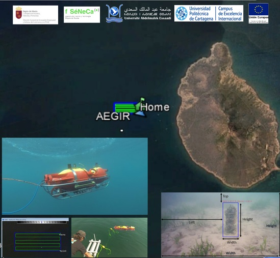
Autonomous Underwater Monitoring System for Detecting Life on the Seabed by Means of Computer Vision Cloud Services

by
Marouane Salhaoui
1,2,
J. Carlos Molina-Molina
1,
Antonio Guerrero-González
1,*,
Mounir Arioua
2 and
Francisco J. Ortiz
3
1
Department of Automation, Electrical Engineering and Electronic Technology, Universidad Politécnica de Cartagena, Plaza del Hospital 1, 30202 Cartagena, Spain
2
Laboratory of Information and Communication Technologies (LabTIC), National School of Applied Sciences, Abdelmalek Essaadi University, ENSA of Tangier, Route Ziaten, BP 1818, Tangier, Morocco
3
DSIE Research Group, Universidad Politécnica de Cartagena, Plaza del Hospital 1, 30202 Cartagena, Spain
*
Author to whom correspondence should be addressed.
Remote Sens. 2020, 12(12), 1981; https://0-doi-org.brum.beds.ac.uk/10.3390/rs12121981
Submission received: 6 May 2020 / Revised: 3 June 2020 / Accepted: 17 June 2020 / Published: 19 June 2020

Abstract

:
Autonomous underwater vehicles (AUVs) have increasingly played a key role in monitoring the marine environment, studying its physical-chemical parameters for the supervision of endangered species. AUVs now include a power source and an intelligent control system that allows them to autonomously carry out programmed tasks. Their navigation system is much more challenging than that of land-based applications, due to the lack of connected networks in the marine environment. On the other hand, due to the latest developments in neural networks, particularly deep learning (DL), the visual recognition systems can achieve impressive performance. Computer vision (CV) has especially improved the field of object detection. Although all the developed DL algorithms can be deployed in the cloud, the present cloud computing system is unable to manage and analyze the massive amount of computing power and data. Edge intelligence is expected to replace DL computation in the cloud, providing various distributed, low-latency and reliable intelligent services. This paper proposes an AUV model system designed to overcome latency challenges in the supervision and tracking process by using edge computing in an IoT gateway. The IoT gateway is used to connect the AUV control system to the internet. The proposed model successfully carried out a long-term monitoring mission in a predefined area of shallow water in the Mar Menor (Spain) to track the underwater Pinna nobilis (fan mussel) species. The obtained results clearly justify the proposed system’s design and highlight the cloud and edge architecture performances. They also indicate the need for a hybrid cloud/edge architecture to ensure a real-time control loop for better latency and accuracy to meet the system’s requirements.

Graphical Abstract

1. Introduction

The world’s seas, as a precious asset and an essential element of its ecology, must be protected as an important source of life, wealth and food. This requires monitoring systems to control their condition and ensure their sustainable management, which involves monitoring physical and chemical parameters related to water quality, such as salinity, temperature, dissolved oxygen, nitrates, density, and chlorophyll levels, among others. Other motives for monitoring the seabed are the detection and conservation of archaeological artefacts and the monitoring of the status of marine flora and fauna, particularly sensitive endangered species [1]. Studies have been carried out in different areas of the Mediterranean, in particular in the Mar Menor, an area of special interest due to its unique environment. The Mar Menor in southeast Spain, with unique salinity and temperature characteristics, is Europe’s largest salt lake, with an area of 180 km2. It is separated from the Mediterranean by a narrow band of sand 22 km long (La Manga), interrupted by several Golas (natural or artificial channels that connect it to the open sea). It has five islands of volcanic origin and is surrounded by several wetland areas. The Mar Menor is a valuable resource with a unique ecosystem and a wide range of habitats for endangered species. It was the subject of numerous scientific studies when recently contaminated chemically and biologically by torrential rains containing large amounts of freshwater and agricultural runoff from surrounding farmland, affecting its flora and fauna [1]. It also sustains considerable phytobenthic and plankton populations during the warm season. All these processes have affected many of its indigenous species.
In the Mar Menor and its surroundings, 27 types of habitats of special interest have been inventoried, eight of which are priorities [2]. Protected species are also abundant and include seagrass meadows (Cymodocea nodosa and Ruppia cirrhosa), marine fauna of special interest, such as seahorses (Hippocampus ramulosus) or the toothcarp (Aphanius iberus), large amounts of fan mussels (Pinna nobilis) and a wide range of marine birds [3]. The fan mussel is an endemic bivalve mollusc, the largest in the Mediterranean and the world’s second largest. The International Union for Conservation of Nature (IUCN) has included Pinna nobilis in its updated list of species in critical danger of extinction from parasitic disease [4].
The Spanish Ministry of Agriculture and Fisheries, Food and Environment, the Spanish Institute of Oceanography, and the Department of Environment of the Balearic Government and the Autonomous Communities of the Mediterranean coast are carrying out studies to protect the fan mussel in areas of Andalusia, Murcia, Valencia, the Balearic Islands and Catalonia [5]. The discovery of some specimens in the Mar Menor in 2019 confirmed that this natural space was a refuge for this threatened species on the verge of disappearing along the entire Mediterranean coast and therefore required monitoring. Although this can be done from manned vessels, this is time-consuming, laborious and expensive and can be done much more effectively by AUVs [6].
AUVs are now widely applied for various tasks, including de-mining, oceanographic investigation, mine clearance and bathymetric data collection in marine and fluvial environments [7]. They are useful for photographing underwater environments and are playing an increasingly important role in marine development [8]. They now dispose of power sources and a smart control system that can carry out autonomously programmed tasks with proper decision making capabilities [1]. Advances in sensor technology, computer technology, new materials and advanced algorithms have significantly boosted their performance, although there are still many issues to be overcome [8,9].
In this paper, we propose and evaluate an AUV system designed to collect and interpret underwater images in Mar Menor to track the fan mussel population in real time, using georeferenced mosaics generated from the images by an automatic processing method.
Besides the challenges and difficulties of an autonomous robot navigating in an unstructured environment, the marine environment has its own particular limitations, not only due to currents but also to the difficulty of geopositioning the submerged AUV. The lack of communication networks and the complexity of connecting to others in real time is also a disadvantage and could be critical not only for transmitting exploration results but also for taking advantage of increased computational capacity and information management when required, such as the artificial intelligence (AI) provided by cloud computing services.
Certain AUV architectures involve the technological challenge of high processing, communication and connection capacity. This requires an architecture that can integrate with a nearby base station, the Internet and cloud architectures. The information gathered during an operation also requires interpretation, which may be crucial for decision making. This means that not only is the local connection important but also the connection with web services (cloud computing, data centres, etc). This latter one can be used to create assistants for a specific purpose and processes to which complex and specific tasks can be delegated.
Distributed control architectures can help to solve many of these issues. These can be incorporated into AUV hardware to speed up the transfer of the collected information to the other side (cloud servers) (Figure 1). Higher intelligence capacity can also help to respond to the needs of the sensor side, especially for very high-speed decision-making, which is impeded by the cloud’s high latency. However, new architectures have recently been proposed to address this deficiency of latency. The present cloud computing system is increasingly unable to cope with the massive amount of data it receives [10]. Edge computing, which is composed of intelligent nodes and could take the place of cloud processing, is expected to solve this issue since it is closer to users than the cloud. These smart nodes range from intelligent gateways to ruggedized outdoor nodes, on-premise heavy storage nodes and edge data center servers.
The main advantage of having a smart node is mainly for local analysis and control, not miles or thousands of miles away, but as close as possible to the measurement point. A quick answer is often required from a smart node instead of high latency, and this justifies having an intelligent node such as edge computing in the same network.
Public clouds have emerged as a new opportunity to deliver compute-intensive applications. A public cloud refers to a networked set of computers that furnish a variety of computing and storage resources and offer the appearance of unlimited computing capacity on demand at a nominal price and under a flexible pricing model [11,12]. DL technology is popular nowadays thanks to its good results in the fields of object detection, image classification and natural language processing. The easy availability of powerful data sets and graphic processing units are the main reasons for DL’s present popularity.
Several smart DL-based applications and services have changed all kinds of people’s lives because of the significant advantages of deep learning in the computer vision (CV) fields [13,14]. CV seeks to enable computer systems to automatically identify and understand the visual world, simulating human vision [15]. Algorithms for visual perception tasks have been developed, including (i) object recognition to identify specific objects in image data, (ii) object detection to locate semantic objects of a given class, and (iii) scene understanding, to parse an image into meaningful segments for analysis [16]. All these algorithm techniques can be deployed in the cloud.
Edge computing is progressively being merged with artificial intelligence (AI) and is intended to migrate DL computation from the cloud to the edge, thereby enabling distributed, reliable and low-latency intelligent services [14]. DL services are implemented nearby the service requests and the cloud is only involved when extra processing is needed [17]. Both the cloud and edge computing are considered adequate platforms to incorporate artificial intelligence approaches. This paper primarily focuses on issues related to the real-time constraints of using AI cloud services and compares DL inference in both environments.
We also propose and evaluate an AUV system designed to collect and interpret underwater images to track the fan mussel population in real time, using georeferenced mosaics generated from the images by an automatic processing method. This automated approach is based on DL image processing techniques such as convolutional neural networks (CNN) to detect the position of a possible specimen in a captured photo. An algorithm on the IoT gateway establishes the connection between the AUV control system and cloud image processing techniques. The results of the suggested system are then compared with cloud image processing methods in terms of latency and certainty.
The rest of the paper is structured as follows. Section 2 outlines the current state of the art and related works. Section 3 describes the proposed AUV-IoT platform. Section 4 describes the AI and vision-based object recognition system. The visual servo control and distance estimation systems are outlined in Section 5, the performance is appraised in Section 6, and Section 7 describes a case study in the form of an exploration project.

2. Related Work

The Internet of Things Ocean (IoT), often described as a network of interconnected intelligent underwater objects, is seen as a promising technology for the systematic management of diverse marine data [18,19,20]. Areas of application for IOT-based marine environmental monitoring comprise: (1) ocean detection and monitoring; (2) coral reef monitoring; (3) marine fish farm monitoring (offshore or open ocean); (4) water quality monitoring; and (5) wave and current monitoring [21].
Underwater robots are widely used in various marine applications: aquaculture [22], visual inspection of infrastructures [23], marine geoscience [24], marine biodiversity mapping [25], recovery of autonomous underwater vehicles [26] and visual monitoring of marine life [27]. Due to their large number of possible applications and high efficiency, AUVs are of significant interest to oceanographers and navies for marine research and reconnaissance. Autonomous marine systems, including AUVs and underwater gliders, are revolutionizing our capability to survey the marine world [28,29,30]. Marine scientists and robotic engineers now have at their disposal a heterogeneous collection of robotic vehicles, including AUVs, deep-sea landing vehicles, unmanned/autonomous surface vehicles, remotely operated vehicles, and gliders/drifters [31]. These robotic vehicles are untethered, self-propelled, self-navigating vehicles that can operate autonomously from a shore or vessel for a period of hours to a few days and carry scientific payloads to perform sampling in the marine environment [32]. These platforms can now move around freely, faster and more easily. They are able to collect significant numbers of images from the seabed in a single deployment [33]. For instance, a 22-h AUV dive can provide more than 150,000 images of the seabed and 65 different types of environmental data [34].
Real progress has been made in modern deep-sea research and development, with recent advances in sensors, microelectronics and computers. Direct vision or camera vision is the simplest way to acquire a wealth of information from aquatic environments and plays a vital role in underwater robots. AUVs equipped with the most recent cameras are now capable of collecting massive amounts of data from the seabed [35]. Computer vision algorithms for underwater robotic systems are attracting attention due to significant advances in vision capacities. This opens up a diverse range of applications, from marine research [36] to archaeology [37] and offshore structural monitoring [38,39]. It could soon be routinely used to investigate marine fauna and flora and will provide a significant increase in the data available for research on biodiversity conservation and management [40].
The previous computer vision systems required a long painstaking process whose results are now insufficient [41]. This process (feature engineering) consists of filters or features designed manually that act as filters on an image. If an image is activated above a certain threshold by certain handcrafted filters, it is given a certain class. This unscalable, inaccurate process requires engineers’ intervention and takes up their precious time [41]. Currently, with effective available cloud services and deep learning algorithms that can be deployed in the cloud, we can put into effect a consistent cloud computing system able to manage and analyze the massive amount of submarine data and images.
Underwater images present specific features that need to be taken into account during their collection and processing. They present a serious challenge and provide an added difficulties and common issues, for instance, scattering, non-uniform lighting, shadows, colour shades, suspended particles, light attenuation and the abundance of marine life [42]. Some of these issues can be handled by underwater image processing methods. Basically, such approaches can be divided into two categories: software-based methods and hardware-based methods [43,44,45]. The authors of [46] propose a stereo-imaging technique for recovering underwater images by considering the visibility coefficients. This stereo-imaging approach was realized using real-time algorithms and was implemented in AUVs. The authors of [47] propose the new Qu index, which is used to assess the similarity of structures and colours in underwater images. The authors of [48] introduce a human perception technique, the High-Dynamic Range Visual Difference Predictor 2, to predict both overall image quality and artefact visibility. The authors of [49] propose a real-time system for object recognition in acoustic images. A 3D acoustic camera is implemented to produce range images of the underwater area [50]. The authors of [51] propose a system for automatic interpretation of 3D objects based on 2D image data generated by a sector scanning sonar unit. Their overall interpretation achieves a success rate of 86% for underwater objects seen in various conditions.
On the other hand, the main constraint on the development of underwater vision algorithms is the insufficient availability of large databases, particularly for DL methods, in which synthetic data sets are usually produced [52,53]. Some data sets are available for object detection [54,55], restoration [56] and visual navigation [57]. Nevertheless, image conditions differ widely between environments, as scattering and light attenuation in water depend on various parameters, such as salinity, water temperature and suspended particles [58]. In fact, the growing trend towards using AUVs for seafloor investigations will only escalate the scientific challenge. Processing the huge amount of data detected by AUVs requires new advanced technologies. Artificial intelligence and machine learning have been proposed to enhance AUV missions and analyse their data. The authors of [59] describe a system for automatically detecting pipelines and other objects on the seabed. Artificial neural networks are applied to classify, in real time, the pixels of the input image of the objects into various classes. The authors of [60] propose CNN to learn a matching function that can be trained from labelled sonar images after pre-processing to produce matching and non-matching pairs. The authors of [61] describe a DL method to assist in identifying fish species on underwater images.
Multiple potential commercial applications and the presence of new open software tools are pushing new advances in AI (e.g., neural networks and DL). As a result, the deployment of AI in scientific research is likely to change [62,63]. New data science software and image analysis can more effectively integrate a variety of tools into the research process, starting from data gathering to the final scientific or public outreach material [64]. AI can assist scientists in shedding new light on the diversity of species living on the ocean floor. Due to significant developments in neural networks and AI, especially DL, computer vision systems can provide remarkable performance in this field of applications. Collaboration between the QUT University of Australia, Google and the Great Barrier Reef Foundation developed the world’s first underwater robotics system specifically designed for coral reef environments. Using real-time computer vision, processed on board the robot, it can identify harmful starfish with 99.4% accuracy [65]. Marine researchers and robotics specialists tested the effectiveness of a CV system in identifying sea creatures and found it be around 80% accurate. The system can even be 93% accurate if enough data is used to train the algorithm [66].
Vision and image processing applications can benefit from cloud computing, as many are data- and compute-intensive. By remotely locating storage and processing capabilities in the cloud, image processing applications can be deployed remotely and paid for by the user in pay-as-you-go or pay-per-use business models. For developers of machine vision and image processing systems, such cloud computing infrastructures pose challenges. While, ideally, cloud-based systems should attempt to automatically distribute and balance processing loads, it remains the developer’s role to guarantee that data is transferred, processed and returned at speeds that satisfy the application’s needs. Several of these implementations adopt algorithms that take advantage of machine learning (ML) and neural networks [67], used to create (i.e., train) the classifiers used by the algorithms. Since real-time creation of these classifiers is not necessary and such training requires significant processing capabilities, it is usually done in advance using cloud-based hardware. Subsequent real-time inference, which implies taking advantage of these previously trained parameters to classify, recognize and process unknown inputs, takes place entirely on the client, at the edge [68]. A hybrid processing topology can be used for some computer vision applications to maximize the benefits of both cloud and edge alternatives [69].
Overall, cloud, edge and hybrid vision processing solutions each provide both strengths and weaknesses; assessing the capabilities of each will allow the selection of an optimal strategy for any specific design situation.

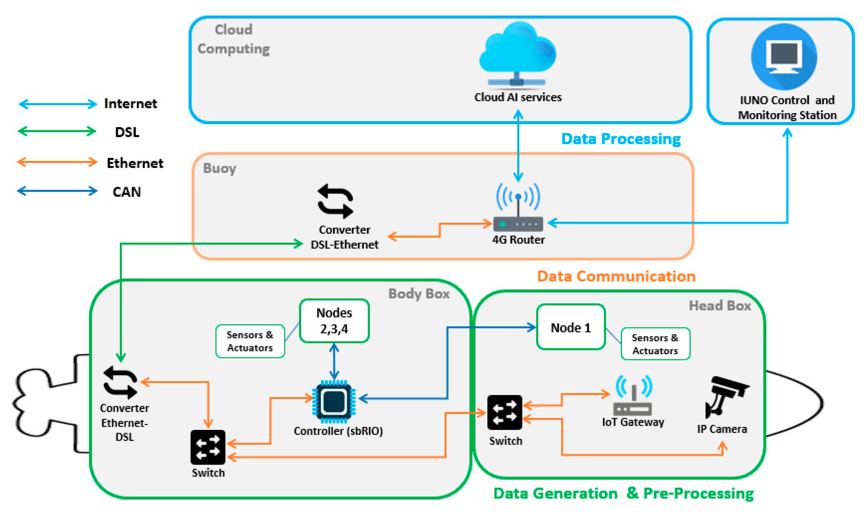
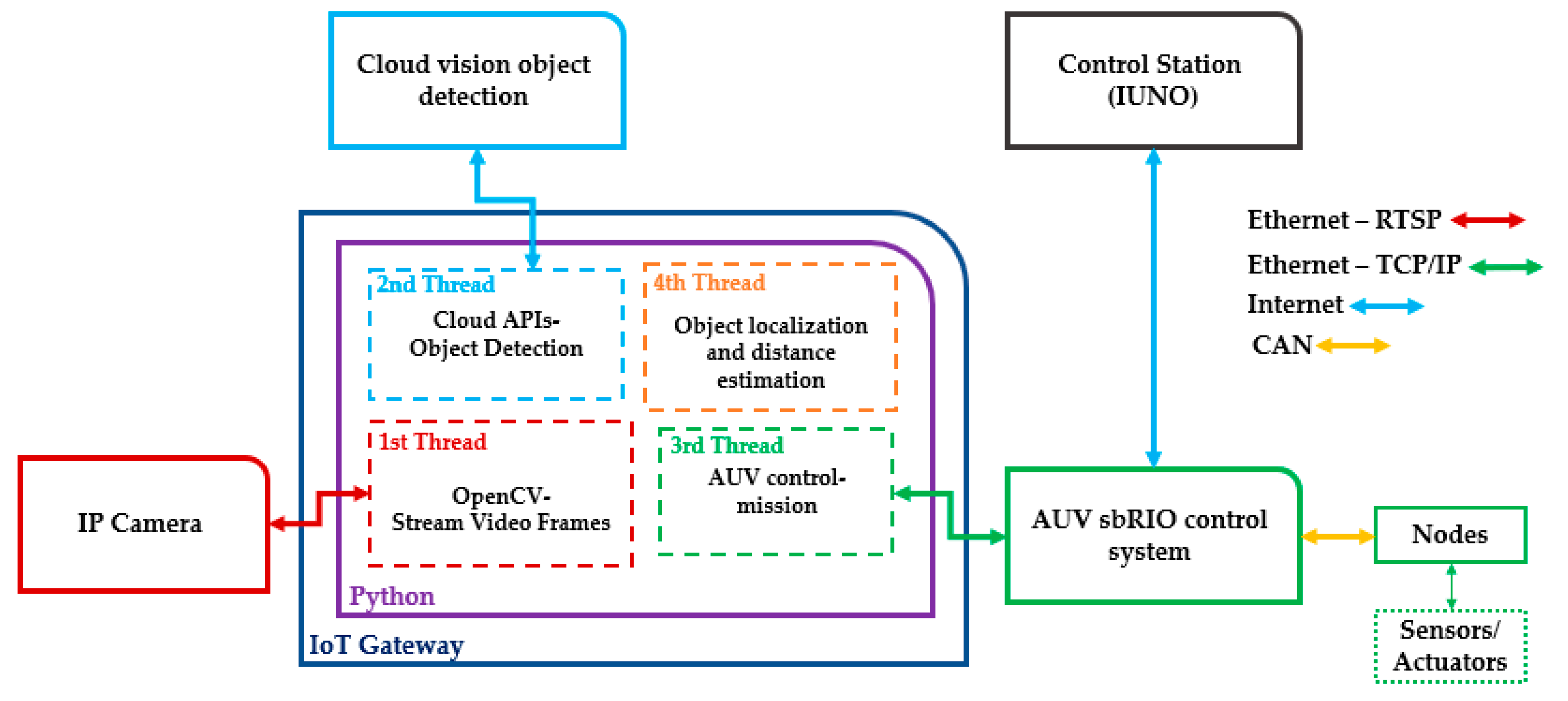
3. Proposed AUV-IoT Platform

The AUV surveillance platform was developed as an autonomous underwater monitoring system to inspect marine life in the Mar Menor (Spain). An approach overview is depicted in Figure 1. The suggested AUV-IoT architecture is structured in three layers, with the AUV in the data generation and pre-processing layer. The first layer involves an AUV composed of different sensors and blocks for data generation, conversion and pre-processing. The pre-processing system is deployed in an IoT gateway installed in the head box and connected to the camera via a switch. The IoT gateway is defined as an edge node. The second layer is the data communication layer with the cloud through Wi-Fi or 4G networks. The last layer is a back-end cloud with image processing techniques.
The three layers are made up of different electronic devices with access to software services. As shown in Figure 2, the physical layer is constituted by a variety of electronic devices interconnected by three different networks according to their functionality: the CAN (controller area network), the Ethernet network and Internet/cloud network. The CAN network is composed of four slave nodes and one master. Each node consists of an electronic card specifically designed for this vehicle and its assigned tasks, and has as a core a PIC 18F4685 microcontroller, working at a frequency of 25 MHz. The main functions of each node are:
  • Node 1 (in the head of the vehicle) manages its movement, lighting, camera power, tilt reading (pitch and roll) and the acquisition of inertial unit variables.
  • Node 2 (DVL: Doppler velocity logger) manages data acquisition and body tilt reading (pitch and roll).
  • Node 3 governs GPS reading, engine management and control (propulsion, rudder and dive).
  • Node 4 monitors marine instrumentation sensors (side-scan sonar, image sonar, microUSBL) and their energy management.
  • The master node consists of a National Instrument single-board Remote Input/Output (NI sbRIO) 9606 (the main vehicle controller). Its function in this network is to collect process information from each of the nodes and send commands. It is the link with the superior Ethernet network.
The CAN network is the field bus for interconnecting the elements dedicated to instrumentation, measurement and actuation. It connects equipment dedicated to specific processes (inputs/outputs, sensor reading, motor control). The CAN network responds to a master/slave configuration, and the elements of this network communicate through the CAN field bus, using the CANopen protocol at a speed of 250 kbps, sufficient for the exchange of process information in real time. This protocol is particularly robust and immune to electromagnetic interference, which makes it ideal for this vehicle.
The Ethernet network allows higher data transfer rates between devices and is formed by the IP camera, IoT gateway, the AUV sbRIO control system and the 4G router. All of these are connected to the buoy through an umbilical cable. Ethernet/DSL (Digital Subscriber Line) gateways are used due to the number of wires in the umbilical cable connecting the vehicle to the surface buoy (only two wires are available for data). As at least four cables are used with Ethernet, and only two with DSL, the Ethernet protocol is converted to DSL before and after the umbilical cable by the DSL to Ethernet gateways. The local bandwidth is 100.0 Mbps, with latencies of less than 1 ms.
The Internet/cloud network allows the vehicle to be connected to the cloud. The 4G router embedded in the surface buoy allows the connection to the cloud. The purpose of this network is the communication of the IoT gateway with the cloud and communication of sbRIO control system with IUNO (Interface for Unmanned Drones) fleet management software. The IUNO software platform was designed at the Automation and Autonomous Robotics Division (DAyRA) of the Polytechnic University of Cartagena. The platform is intended to manage the integrated control of multiple unmanned marine vehicles with the aim of simplifying maritime operations. The results obtained from each vehicle, regardless of its characteristics, facilitate the success of the operation with a high degree of automation [1]. AEGIR is the name of the AUV developed by DAyRA, and it is the main vehicle used in this paper; its structure is described in Figure 2.
There follows an insight description of the critical elements related to edge/cloud computing and the vehicle’s core control system: first, with an in-depth description of the edge node, the IoT gateway, the main AUV controller, and the mission management.

3.1. The AUV-IoT Architecture Development

In this section, we outline and itemize the development of the above-mentioned IoT-AUV autonomous system and its network protocols, portraying five main blocks, namely, the IoT gateway, the IP camera, the AUV control system, the AUV control station and the cloud.
The overall mission is triggered in the AUV control station by setting the desired waypoints and activating the AUV engines and IP camera streaming. The IoT gateway in the head box connects the AUV nodes and the IP camera with cloud services. The IoT gateway receives image data from the IP camera in the submarine’s head box and sensor data from the body box. Likewise, the IoT gateway seizes the image processing results from the cloud for each sent photo. If a fan mussel is detected, the results contain its delimitation box in the image and the percentage of image accuracy. When a fan mussel is detected using the cloud API (Application Programming Interface), the IoT gateway links up with the main controller to modify the submarine’s mission and track the specimen detected. The submarine’s new mission is based on the results received from the cloud API and the algorithm processed in the IoT gateway. The algorithm implemented in the IoT gateway is in charge of adjusting AUV movements to keep the targeted specimen in the centre of the field of view. The distance to the detected specimen is computed using the cloud API and a triangular similarity algorithm [70,71] (Section 5).
The desired mission modifications are routed to the main controller to handle the engines and vehicle heading. In this case, the AUV’s manual tracking control is replaced by an automatic specimen detection system using the cloud APIs and the distance measurement algorithm implemented in the IoT gateway. A specific area is explored based on a specific mission with settled waypoints. The tracking algorithm in the IoT gateway is triggered automatically if the forward camera detects a specimen (Figure 3).
The IoT gateway’s main function is to acquire the camera image, timing the shot according to the AUV’s depth and speed, to obtain photographic mosaics with overlapping images. The IoT gateway receives the captured images and forwards them to the cloud, which uses advanced learning techniques to analyse the results and send them to the IoT gateway. The obtained results from the cloud are exploited to adjust the new underwater mission to pinpoint the specimen’s exact location. This is described in Algorithm 1, as well as in the flowchart in Figure 3.
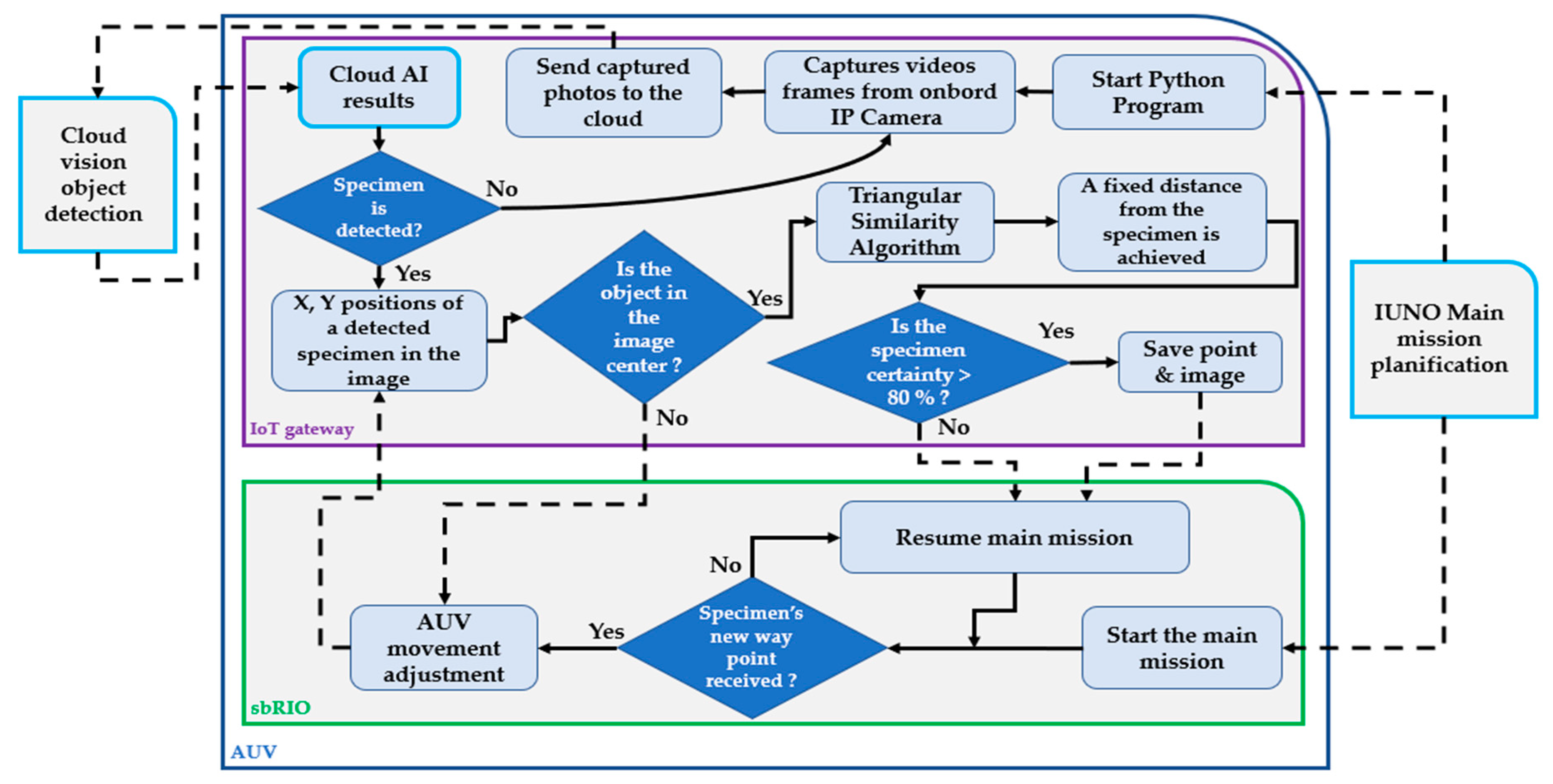
Algorithm 1. Specimen tracking algorithm
Start ()
Step 1:
   While (mission has not started) {}
Step 2:
   If (mission has ended)
     {End()}
   Else
     {Acquire frame and send to cloud}
     {Get the answer}
     If (accuracy > 20%)
        {Go to step 3}
     Else
        {Go to step 2}
Step 3:
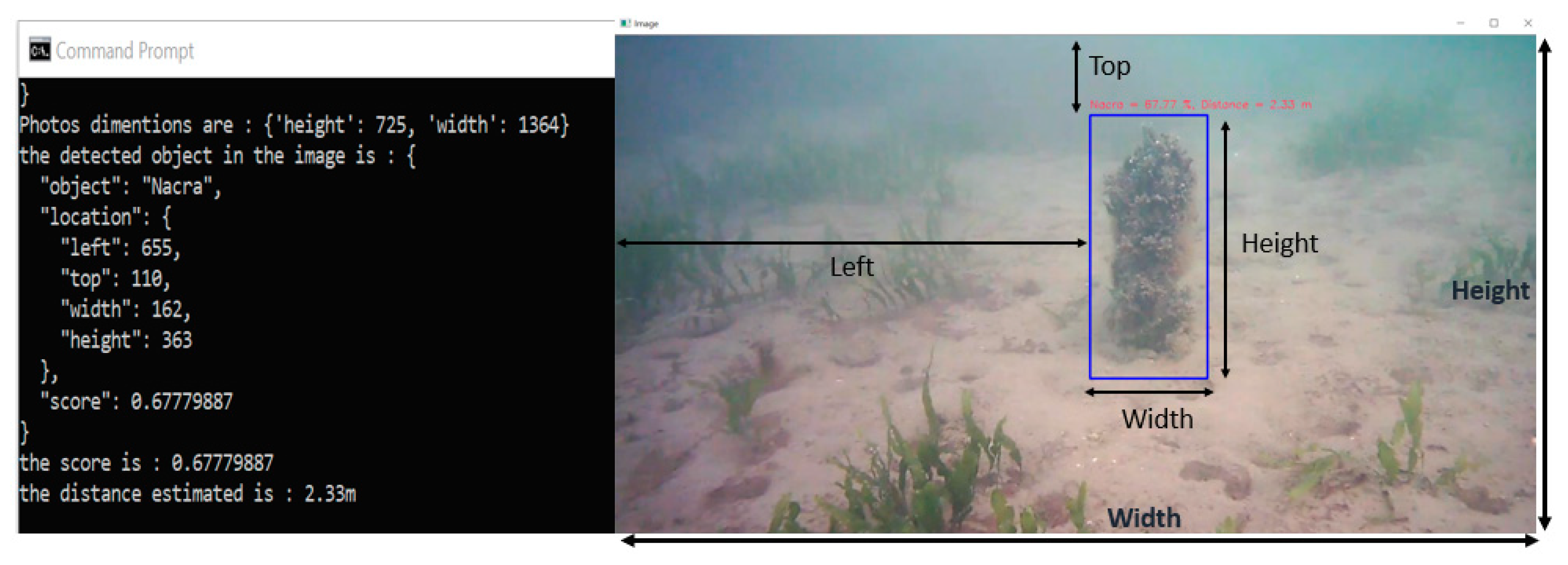
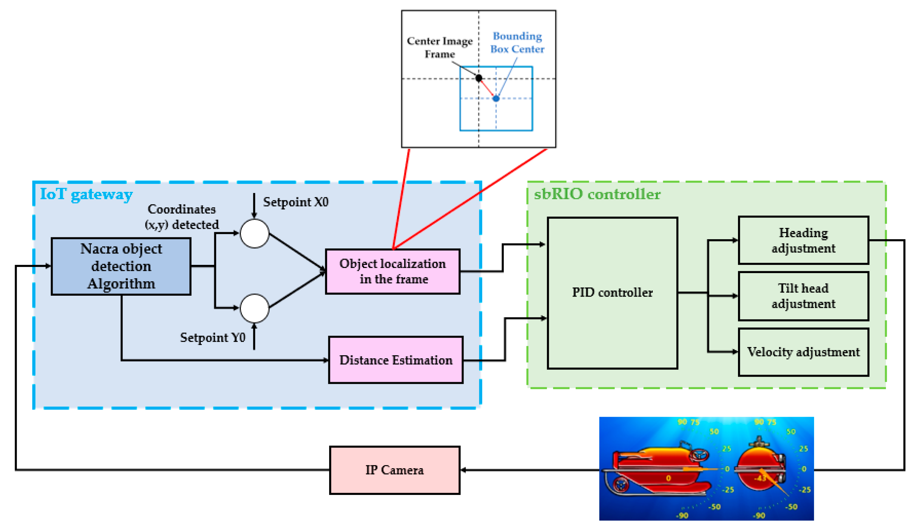
   {Calculate the bounding box centre of detected object}
   {Calculate the distance between the centre of the detected nacre bounding box (C1) and
     the center of the captured frame (C2)}
   {Conversion of distance (C = C2C1) into degrees (new heading and tilt setpoint)}
   {Send command to sbRIO with new heading and tilt setpoint.}
   If (C==0)
      {Go to step 4}
   Else
      {Go to step 3}
Step 4:
   {Send the command to sbRIO to set the speed (fixed speed setpoint)}
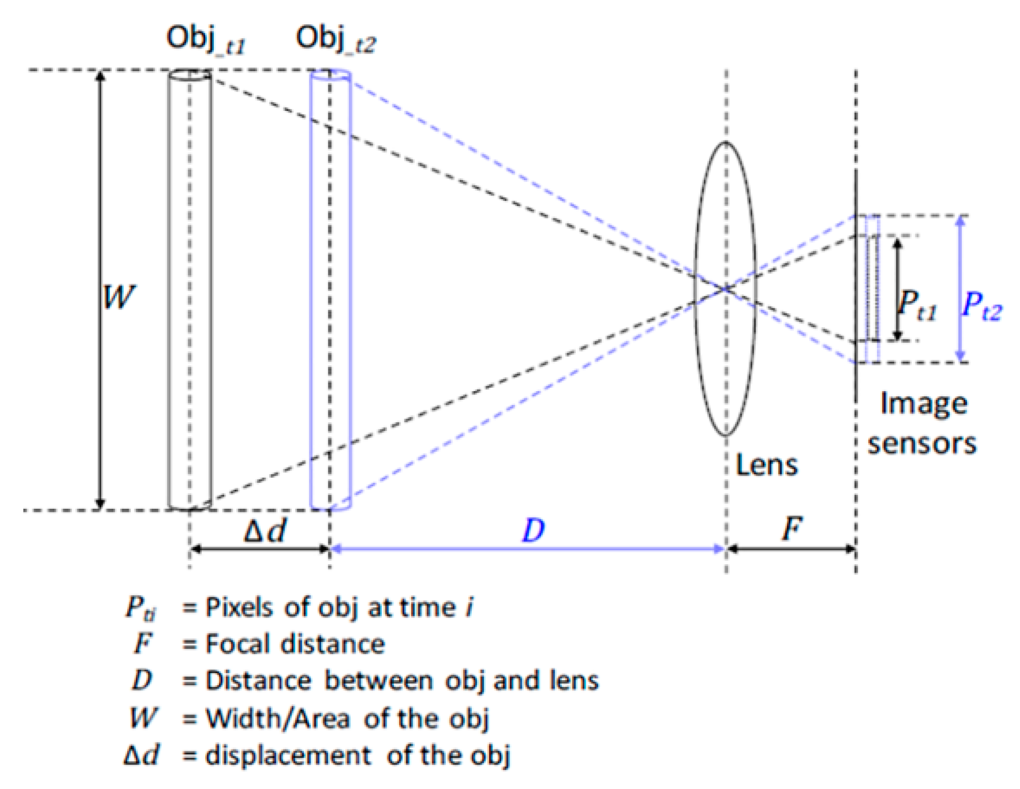
   {Take images I1 and I2 in two different positions, where P1 and P2 are the pixel widths
     of the objects detected in both images}
   {Calculate the distance using the following equations.
D + Δ d = ( W × F ) / P 1
  D = ( W × F ) / P 2  
   where F = 2.34 mm is the focal distance, W is the width of the real detected object
   If (the distance D calculated > 2 m)
      {Go to step 4}
   Else
      {Go to step 5}
Step 5:
   {Get accuracy of the specimen image}
   If (accuracy ≥ 80%)
      {Save point, save picture and resume mission}
      {Send command to sbRIO to save specimen’s position}
   Else
      {Go back to the main mission without saving. It is not a specimen}
      {Go to Step 2}
End ()

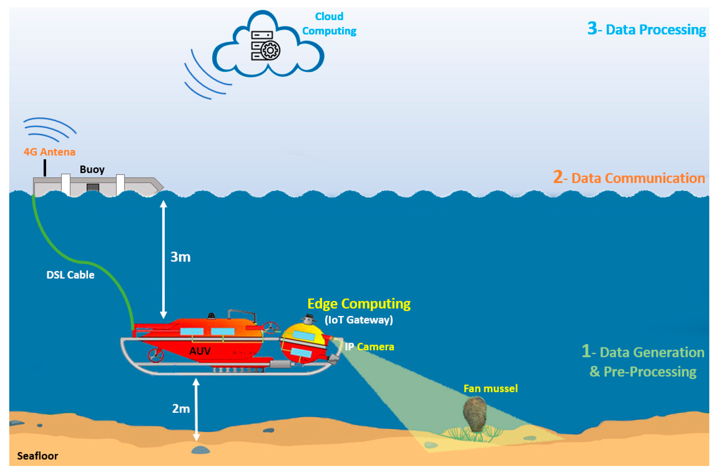
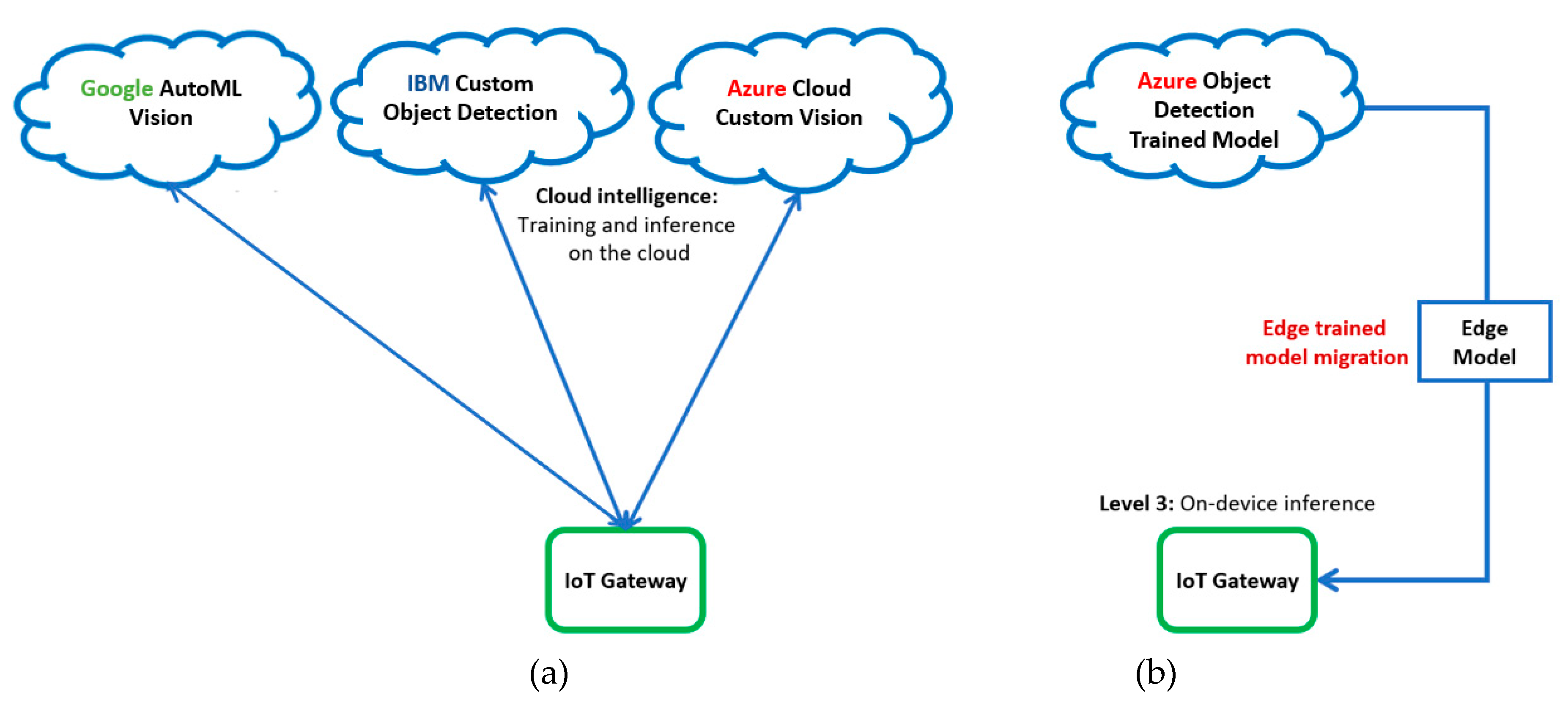
3.2. IoT Gateway: The Edge Node and Connection to the Cloud

The implemented IoT gateway is capable of connecting the sensor network to the cloud computing infrastructure, performing edge computing and serving as a bridge between the sensor networks and the cloud services [72]. Experiments were carried out using Python installed in the IoT gateway. The Python program employed serves as an interface to communicate with the submarine sensors and actuators, the cloud computer vision APIs and the underwater controller (Figure 4). Python has a built-in support for scientific computing. Its use is growing fastest in data science and machine learning [73]. Versatility, the stability of libraries with great support, and ease of use are its main benefits [74]. The IoT gateway also features Open-source Computer Vision (OpenCV) which is a library of programming functions mainly for real-time CV. In our application, OpenCV is used for live video streaming over an Ethernet network connected to the prospective IP camera (model Sony SNC-CH110) installed in the head box. All the Python cloud libraries required for image recognition are installed in the IoT gateway.
Whereas the Python program in the IoT gateway is started (Algorithm 1), connection is established with the camera by the Real-Time Streaming Protocol (RTSP). The Python program in the IoT gateway is executed to run four threads (tasks) at the same time (Figure 4).
The first thread is tasked with capturing and streaming video images from the IP camera to the IoT gateway internal memory. If a specimen is detected using the cloud object detection service, the AUV’s movements are adjusted to focus the camera on the object. The distance between the detected specimen and the vehicle is computed in the IoT gateway and employed to steer the AUV to track its position. The AUV’s heading and mission control commands are routed via TCP/IP (Transmission Control Protocol/Internet Protocol) to the sbRIO controller in the head box, which is connected to several nodes via a CAN bus protocol. Each node is connected to a different group of sensors and actuators.
The cloud service used in this case is the vision object detection service, which allows training of customized machine learning models that are able to detect individual objects in a given image along with their bounding box and label. There are many different cloud APIs for computer vision, e.g., IBM, Google, Microsoft Azure and Amazon. They all provide fairly similar capabilities, although some emphasize object recognition, Amazon, or building custom models, like Microsoft Azure and IBM. The strength of these cloud APIs is their ability to develop custom models rapidly and download trained custom models to deploy them on the edge for real-time applications and low-latency requirements [75,76].
To appraise the effectiveness of the suggested platform, we assessed its overall latency, in order to act quickly when an underwater specimen is detected and control the AUV mission according to the cloud results of each photo. The Python program is divided into four threads; however, the response time of the cloud services takes significantly longer, depending on different factors. Figure 4 presents the connection between the IoT gateway and the different systems. Each thread of the IoT gateway is responsible for synchronously triggering a task and ensures maintenance of the connection.

3.3. AUV Control

The most relevant characteristics of the AUV used in the experiment are as follows: the vehicle is physically divided into two compartments (head and body), consisting of five thrusters (two for propulsion, two for depth control and one for the rudder) and weighs 170 kg. This vehicle is capable of submerging to 200 m and has 7-h autonomy. Its two battery blocks (one supplies power to the electronics and sensors and the second to the thrusters) are reconfigurable to 24 V for greater autonomy or to 48 V for greater power and cruising speed. It can move at 4 knots and perform long-term missions while locating and identifying submerged targets, photogrammetry and sonar inspection of the seabed. It is equipped with the following devices: image sonar, side scan sonar, micro-USBL (UltraShort BaseLine) for acoustic positioning, an inertial unit, GPS (Global Positioning System), a DVL (Doppler Velocity Logger) for measuring underwater movements, a camera and a depth meter.
As shown in Figure 4, our underwater vehicle has a number of elements and devices interconnected through different networks. While the IoT gateway is in charge of recognition and communications with the camera and the cloud, the sbRIO controller is the AUV’s main control backbone. The National Instrument sbRIO 9606 embedded controller integrates a real-time processor with a reconfigurable FPGA through its LabVIEW environment [77,78,79]. It comprises Ethernet, CAN and I/O connectivity, as well as a 400-MHz CPU, 256 MB DRAM, 512 MB storage, and other features listed in [77,78]. A consistent code for the sbRIO controller was fully developed in the LabVIEW environment for AUV management, control and command.
The modules in the sbRIO’s vehicle control program comprise these operations:
  • CAN bus (reading and writing interface): There are a number of nodes connected to the vehicle’s CAN bus, whose network master is the sbRIO. Each of the nodes has a series of sensors and actuators connected. The function of these blocks is to receive information and send commands to the different nodes through the CANopen protocol. The type of data received or sent will depend on the function of the node.
  • TCP/IP (reading and writing interface): This manages TCP/IP communications for receiving commands from IUNO and the IoT gateway, as well as sending navigation information from the vehicle to the rest of the equipment on the Ethernet network.
  • Data manipulation: This is responsible for adapting the data formats from the different sources (CAN, inertial unit, IUNO) to a common format within the program and vice versa: e.g., conversion of latitude received through the CAN network interface (UINT8 array type, extracted from a buffer) to I32 data type.
  • Data saving: This saves the process and navigation information in the sbRIO in TDMS (Technical Data Management Streaming) format files. TDMS is a binary measurement file format, focused on storing information in the smallest possible space. It can be exported to several formats (csv, xls, txt, etc.).
  • Heading control/depth control/velocity control/heading tilt control: Management of the different control loops for heading, depth, velocity and head tilt. These take on special importance in automatic or semi-automatic navigation modes.
  • Thruster control: As a result of the previous timed loop, a heading, depth or position setpoint is obtained. In this module, they are processed to obtain as a result a PWM (Pulse-Width Modulation) value to be applied to each of the vehicle’s engines.
  • Automatic (IUNO)/manual mode navigation: AEGIR developed at the Division of Automation and Autonomous Robotics (DAyRA) of the Polytechnic University of Cartagena, and the Ocean Server AUV IVER2. IUNO’s capabilities and characteristics. An AEGIR vehicle can be handled in both modes: manual and automatic. This timed loop is in charge of selecting the appropriate navigation source. Only the automatic mode is considered in this paper.
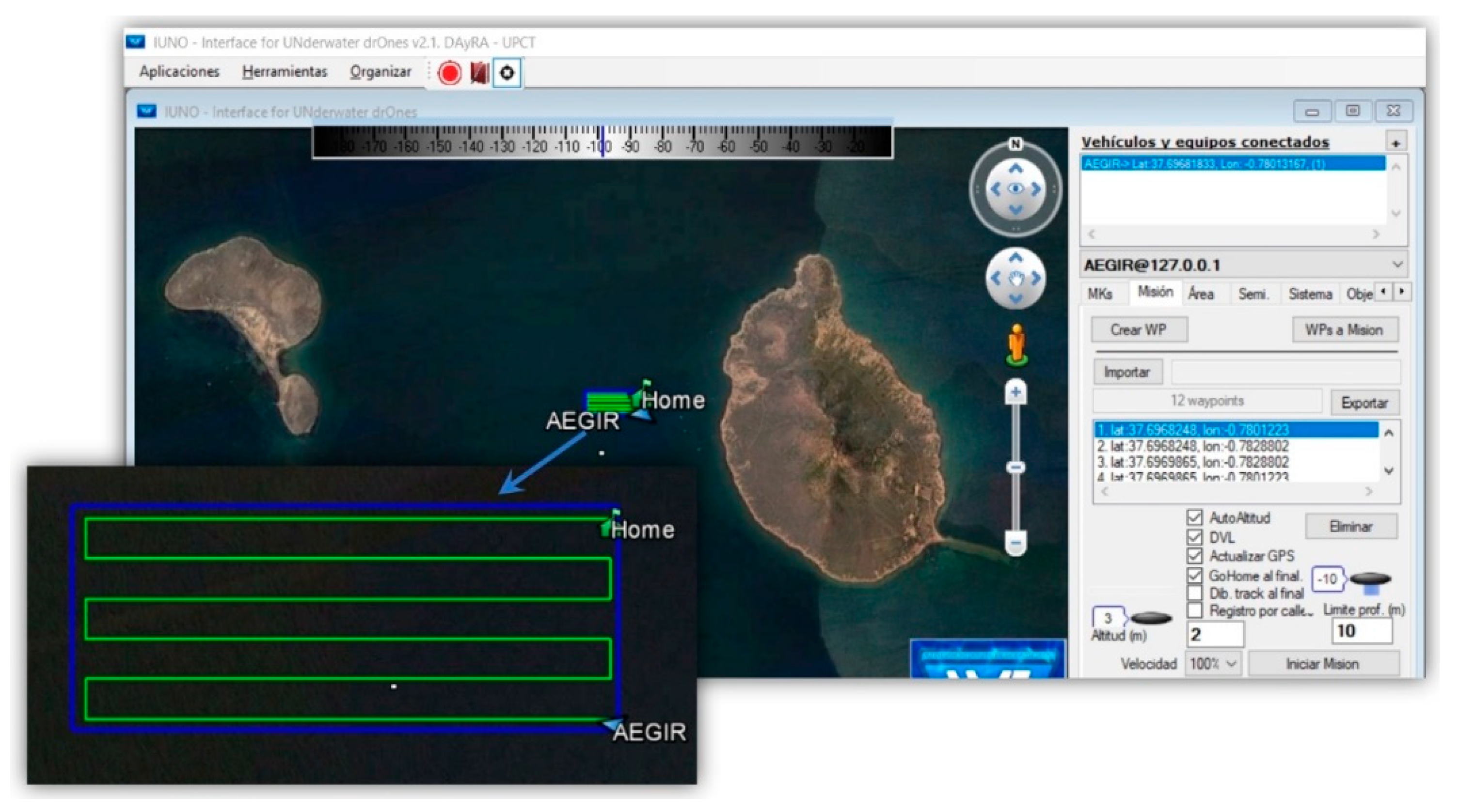
  • Mission management: Once the mission created in IUNO is downloaded, this module manages each of the waypoints to which the vehicle must navigate, dispatching the different navigation commands for the heading control/depth control/position control timed loops. This module also handles the main navigation mode in normal operations and the specimen tracking navigation mode, as described in Section 7.

4. Artificial Intelligence and Vision-Based Object Recognition

4.1. Deep Learning for Object Detection

In the last decade, prominent applications like robotics, video surveillance, scene understanding, and self-driving systems have initiated a significant amount of computer vision research. Thanks to the advancement of neural networks, particularly deep learning, visual recognition systems have achieved impressive outcomes, especially in object detection.
Object detection is the process of identifying the instance of the class to which the object belongs and estimating its location by outputting the bounding box around the object [80]. Although object detection and image classification both share a common technical challenge, they must handle significant numbers of highly variable objects. Object detection is more complex than image classification due to the fact that it must identify the precise location of the object of interest [16]. Being one of the main computer vision issues, object detection is capable of providing useful insights for the semantic understanding of images and videos [81]. Object detection, i.e., the detection of the positions and categories of multiple instances of objects in a single image, is a major challenge in a diverse set of applications such as self-driving vehicles and robotics [82,83,84].
Object recognition efficiency is steadily increasing, with advanced computer vision techniques working successfully on a wide range of objects. Most of these techniques are based on deep learning with convolutional neural networks, and have achieved impressive performance improvements in a variety of recognition problems [85].

4.2. Convolutional Neural Network for Object Recognition

Applying computer vision to automatically detect objects is an extremely challenging task. Noise disturbance, complex background, occlusion, scale and attitude changes, low resolution, and other factors strongly influence object detection capabilities. Conventional object detection methods, based on the hand-crafted feature, are not robust to lighting changes, occlusions and variations in scale or lack of good generalization ability [86]. Unlike handmade features, which are designed in advance by human experts to extract a particular set of chosen properties, the features extracted by CNN are learned from the data. The core idea behind this is to learn object models from raw pixel data rather than using hand-set features, as in traditional recognition approaches. Training these deep models usually requires large training datasets, although this problem has also been surmounted by new large-scale labelled datasets such as ImageNet [87].
CNN-based methods have achieved significant advances in computer vision. In the 2012 ImageNet Large Scale Visual Recognition Challenge (ILSVRC) [88], Hinton and his student Krizhevsky [87] applied CNN to image classification and achieved a winning top-5 test error rate of 15.3%, compared to the 26.2% achieved by the second-best entry. Applying various convolutional filters, CNN models can capture the high-level representation of the input data, making it highly popular for CV tasks. The breakthrough and rapid adoption of DL in 2012 brought into existence modern and highly accurate object detection algorithms and methods, such as the regions with CNN features (R-CNN) method [89], fast R-CNN [90], faster R-CNN [91], RetinaNet [92] and fast yet highly accurate methods like SSD [93] and YOLO [13]. CNN-based methods can provide more accurate target boxes and multi-level semantic information for identification and localization. However, handcrafted features are complementary and can be combined with CNN for improved performance [94].
By using the cloud infrastructure, it becomes possible to apply CNN techniques which are used in most object detection cloud services [80]. There are two ways that can help leverage these techniques for a particular application. The first one consists of employing our own data and a framework in our own machine and training our custom model for custom object detection. The second is to use cloud services through an API, which is a suite of machine learning (ML) products and CV software development services that allows developers with limited ML expertise to train high-quality models specific to the needs of their project.

4.3. Object Detection Training in the Cloud

Besides the general object detection models provided by cloud services, certain others can be used to create their own custom object detection model to identify items and their location in an image. Object detection models can be trained to recognize objects that are important to the user in specific domains. Object detection training data is the set of object labels and locations in each trained image. The tag or label identifies what the object is. The location identifies where it is in the image. It is also possible to identify more than one object in an image. Cloud services offer users a friendly interface to develop and deploy custom CV models. We identify the location by drawing a bounding box around the object and providing the top and left pixel coordinates of that box, along with the width and height in pixels (Figure 5).
In the case study, we trained about 90 photos on the same data set in Azure, Google and IBM Watson cloud services, all of which offer nearly the same service for custom object detection. The training photos are a mix of our own photos and others from Creative Commons sources [95] (Figure 6). The system is very similar to custom classification, except that this service identifies the location of the items in the image. The response also includes a classification label for each item detected and an identification confidence score.
After creating a custom object detection model and completing the training, we tested its fan mussel detection capacity in other images using the Python cloud API, as shown in Figure 7.
The trained vision model successfully identified a new specimen in the image and also its location and its probability percentage score. The blue bounding box is drawn by the Python program using the results received from the cloud. According to the results and the AUV navigation sensor data, the proposed Algorithm 1 can estimate the distance between the AUV head box and the detected specimen.

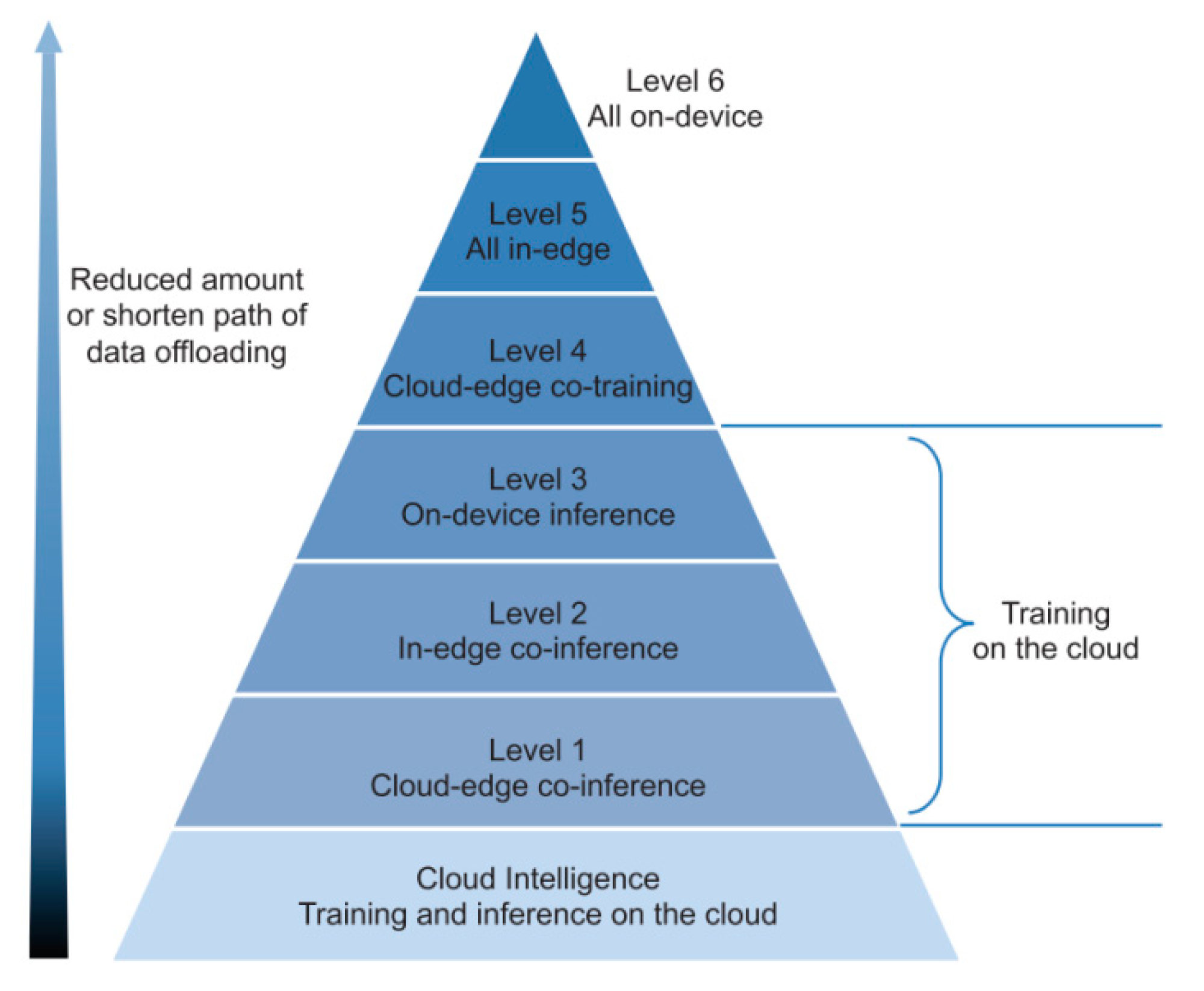
4.4. The Cloud AI at the Edge

The Mar Menor, as the largest saltwater lake in Europe with a wide range of flora, requires constant monitoring. The 4G network covers the entire zone and connects a large area to the Internet to take full advantage of cloud computing services. As described above, AUVs are a complete fan mussel monitoring system thanks to being interconnected to the latest cloud computing services.
The advantages of cloud-based API services include simplified training and evaluations to improve and deploy models based on our own data. However, despite its advantages, edge computing has certain drawbacks, including privacy protection, context awareness, low latency, bandwidth consumption and energy efficiency [96,97].
To address these challenges, edge computing has recently been envisioned to push cloud computing services closer to IoT devices and data sources. Edge computing is designed to drive low-latency data processing by migrating computing capacity from the cloud data centre to the edge [75,76]. Influential cloud computing vendors, such as Google [98] and Microsoft Azure [99], have released service platforms to drive intelligence to the edge, allowing end devices to execute machine learning inference locally with pre-formed models.
Figure 8 describes the six different ways of using edge intelligence for ML applications, in which the edge can be combined with the cloud or used alone for the entire application process. In this paper, we adopt two main methods: the cloud intelligence method, in which training and inferencing are both performed in the cloud, and the Level 3 method, with on-device inference and cloud training.

5. Visual Servo Control and Distance Estimation

Visual servo control consists of computer vision data usage to control the AUV’s motion [100]. Related works on underwater vision tracking and visual servo control for autonomous underwater vehicles have shown that vision and visual servo control are imperative in developing AUV systems, as the vision–AUV combination yields substantial benefits. Several studies on underwater tracking focus on visual servoing, such as autonomous alignment and dynamic positioning [101,102], pipeline following and planet target tracking [103]. With the advent of machine vision and deep learning, it is currently viable to specify the object to be tracked. ML object tracking has already been tested in different underwater applications, such as fish tracking and diver following and tracking [104,105].
To perform underwater vision tracking in Mar Menor and track the underwater Pinna nobilis species, the fan mussel tracking algorithm is solved using the object recognition cloud API incorporated in the AUV control loop. Through this algorithm, we verify that a specimen has been detected, and from there we calculate the coordinates of its center (x, y). In this scenario, the AUV reduces speed, and a PID (Proportional–Integral–Derivative) controller will keep the object in the centre of the frame by adjusting AUV yaw and head tilt to keep the camera centred on the object detected [106,107].
When more than one specimen is detected, the system follows the one with the highest score. The x and y coordinates are adopted as information in the object tracking process. To make the system effectual, the port and starboard engines and AUV head tilt are adjusted to track the object using the object’s coordinates as feedback. The thrust motors follow the position changes of the object’s coordinates by means of PID controllers. When the detected object is centred, its distance from the AUV camera is computed using the cloud API results and a triangular similarity algorithm [70,71]:
D = ( W × F ) / P
where P is the width of the object in pixels and W is the width of the object itself.
The camera focal distance F is fixed and the apparent P is obtained from the cloud results. To obtain W and estimated distance D, a minimum of two pictures are required at different distances from the object for calibration, as presented in Figure 9 and Algorithm 1.
( D + Δ d ) × P t 1 = D × P t 2 = W   × F
D = ( Δ d × P t 1 ) ( P t 2 P t 1 )
The cloud object detection API and the tracking algorithm are fully implemented using Python. The entire Python program is processed in the IoT gateway while yaw and tilt are processed in the sbRIO main controller. The output data coordinates from the cloud are used to keep the AUV automatically focused on the object itself in the desired position.
The sbRIO main controller drives the robot’s movements to keep the target’s bounding box in the centre of the camera image. The IoT gateway continuously sends coordinate errors (distance, X position, Y position) to this controller, so that these data become the input for the closed loop for tilt, heading and speed adjustments (Figure 10).
Figure 10 presents the modules and process involved in detecting and tracking the target. In the object detection algorithm block, the system aims to keep the target in the centre of the image. When the relative size of the target has been obtained from the object detection API, these control loops are kept operative while the speed is gradually increased to calculate the estimated distance by means of the similarity triangulation algorithm. From then on, tilt, heading, speed and control loops keep the target in the centre until the vehicle is at the desired distance. The tilt and heading closed control loop were successfully tested in calm waters and slow currents, although difficulties were encountered with stronger currents.

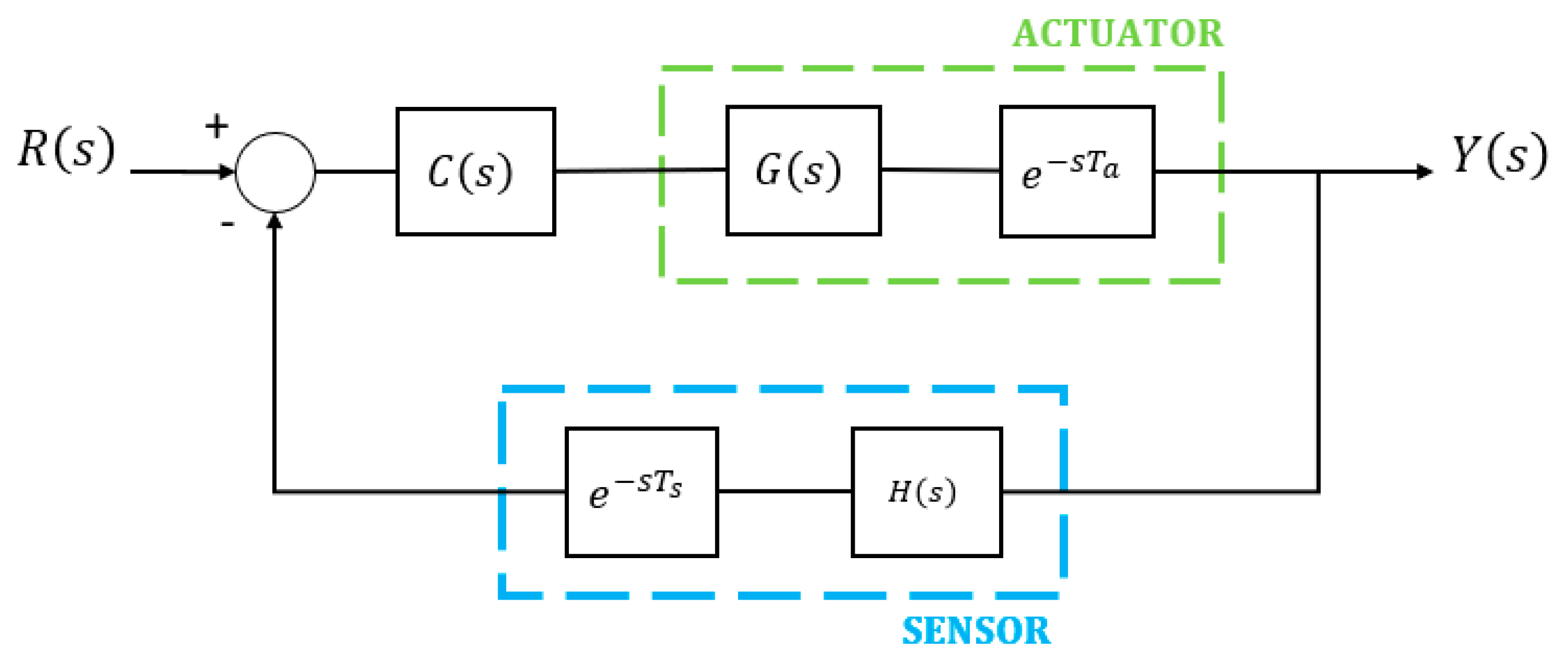
Servo Control Latency

The visual system is required to provide real-time results from the control loop with very low latencies. The principal concern is the ability to detect the target and aim the camera at the centre of the image. To obtain effective real-time control, the delays involved in initially detecting the target and those of the sensor and actuator while tracking the object must be minimised (Figure 11) [108]. Three distinct types of delay are involved. The first is actuator delays, which occur in the feedforward loop when the delay is in the robot itself. The second type is sensor delays in the feedback path of a closed-loop system, derived from a sensor delay. This delay is present in any real-time control system with visual feedback and depends on the amount of visual processing required. The third type is transportation delays, or pure time delays, usually due to long-distance communications.
To reliably assess the servo control latencies, we modelled the basic closed-loop system with sensor and actuator delays, as shown in Figure 11. Y(s) is the output signal and R(s) is the reference signal. The sensor and actuator delays are represented, respectively, as e s T s and e s T a   in the frequency domain, the (undelayed) sensor dynamics by H(s), the (undelayed) plant dynamics by G(s), and the controller by C(s).
The most important delays in a control loop with visual feedback are those caused by the sensor, and the delay time directly affects the dynamic stability of the control system. System stability is determined by the poles of the input/output transfer function, i.e., the roots of the denominator. For a single-input–single-output (SISO) system, the denominator (characteristic equation of the system) is simply 1+ the loop gain, so that any stability analysis would incorporate the total actuator and sensor delay to determine stability bounds.
Y ( s ) R ( s ) = C ( s ) G ( s ) e s ( T a ) 1 + C ( s ) G ( s )   e s ( T a ) H ( s )   e s ( T s )
and the characteristic equation is:
1 + C ( s ) G ( s ) H ( s )   e s ( T a + T s ) = 0  
The effects of stability can be analysed by studying the conditions of marginal stability. From the above equation, the following expressions are deduced:
| C ( j ω ) G ( j ω ) H ( j ω ) | | e j ω T | = 1
L ( C ( j ω ) G ( j ω ) H ( j ω ) ) L ( e j ω T ) = 180 °
As e j ω T = 1 for all ω , the magnitude of the system is not affected by the delay. However, as L ( e j ω T ) = ω T radians, it is clear that the phase margin for a system with a time delay decreases as the time delay increases, leading to instability and thus constraining the bandwidth achievable in the face of delays.
One way to deal with the pernicious effect of known or unknown delays is to detune first-order gains. With a PID controller, this is performed by reducing the proportional gain (P) to levels where the system remains stable. This approach has the disadvantage that the resulting response is slowed down and, therefore, the overall performance of the system is worsened. The servo control must ensure a compromise between performance and stability. The performance is proportional to the value of the gain of the corrector; however, above a certain value, the corrector tends to destabilize the system.

6. Performance

Cloud and edge computing are considered adequate platforms to incorporate artificial intelligence approaches. This paper primarily focuses on the issues related to the real-time constraints of using an AI cloud in both environments. Our AUV system is designed to collect and interpret underwater images to track the fan mussel population in real time by an automatic processing method. This automated approach is based on DL image processing techniques, such as CNN, to detect the position of a possible specimen in a captured photo. The IoT gateway algorithm establishes the connection between the AUV control system and cloud image processing techniques. The results of our proposed system are compared with cloud and edge image processing in terms of latency and certainty. Therefore, we aim to compare the response time between the cloud and edge inference.
Microsoft Azure cloud was first compared with IBM and Google clouds, as shown in Figure 12 [98,99,109]. The second comparison evaluated the same cloud service with inference in the edge and comparing the same results in the cloud.
We describe the various network connections and the performance metrics for the architectures given in Figure 12. We first assessed the delay between the different terminals in the cloud architecture and then compared it to that of the edge computing architecture. We evaluated the performance of each trained model in the cloud and in the edge. Below, we compare the performance of each architecture, using LattePanda as an IoT gateway, with a 1.8-GHz Intel quad-core processor, 4 GB RAM and 64 GB on-board flash memory.

6.1. Delay Assessment in the Proposed Platforms

Figure 13 and Figure 14 exhibit the different data flows via the various communication networks for the cases of cloud and edge computing. From data acquisition (sensors) to actuators, the information flow goes through different networks: CAN and Ethernet in the case of edge architecture, and the Internet and DSL for the cloud architecture. This represents the difference in latency between the two modes and highlights the critical points in each case. The highest latency expected in the case of edge computing is Tinference, and the Tcloud is the one expected in the cloud.

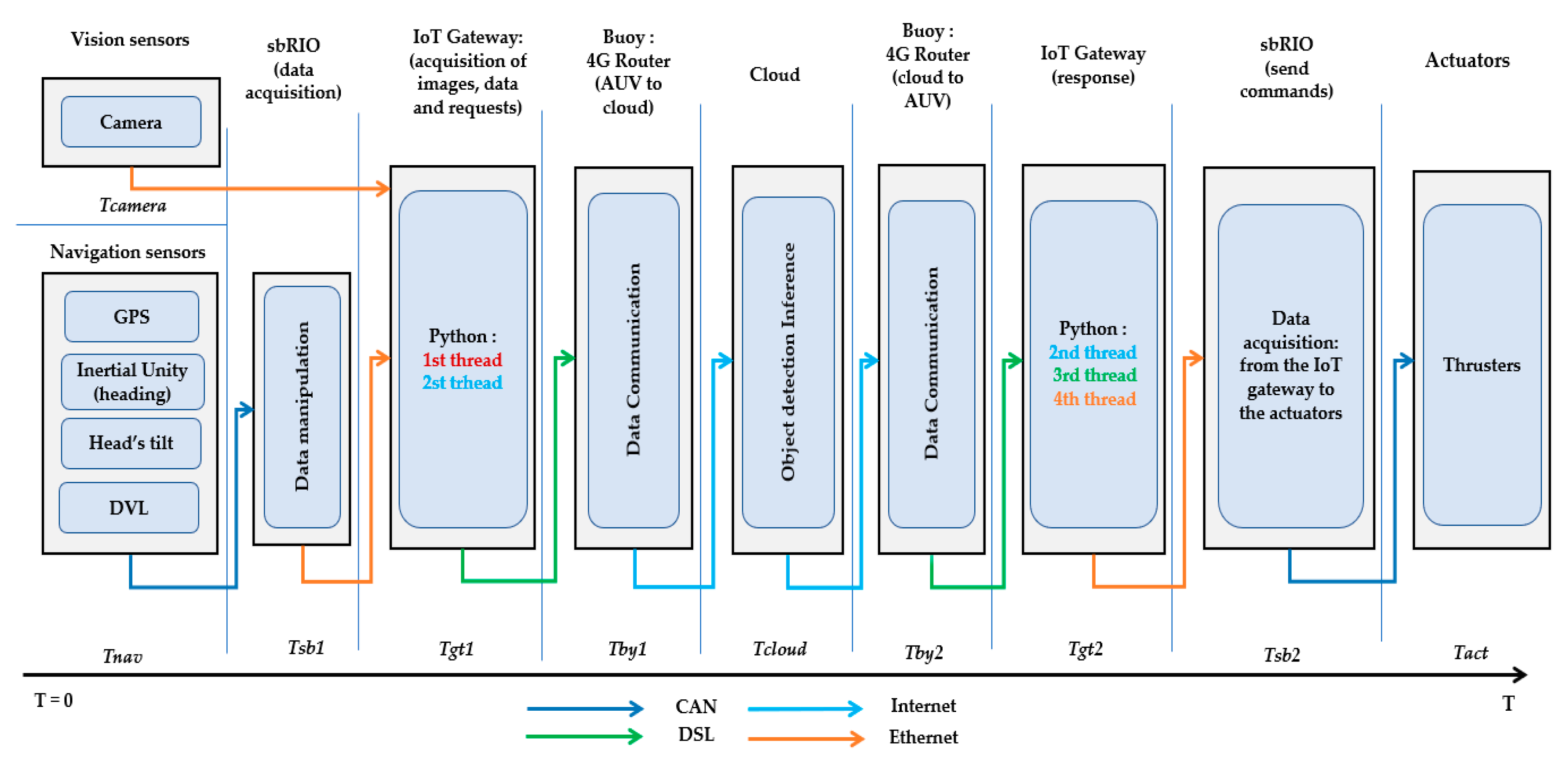
6.1.1. Cloud Architecture

In the adopted cloud architecture, all the generated images are sent to the cloud services and the inference is performed entirely in the cloud. This makes the application fully dependent on the cloud results in order to make the necessary adjustments, which are crucial in the case of intermittent connectivity. Figure 13 shows the different delays in the use case process.
The response time in the system can be divided into delays, as modelled in Equation (8):
T = T n a v + T s b 1 + T g t 1 + T b y 1 + T c l o u d + T b y 2 + T g t 2 + T s b 2 + T a c t
where:
(1)
Tnav is the navigation sensor time,
(2)
Tsb1 is the acquisition time of the sensor data in sbRIO,
(3)
Tgt1 is the processing time of the first and second threads in the IoT gateway presented,
(4)
Tby1 is the transmission time from the AUV to the buoy,
(5)
Tcloud is the time needed to send photos to the cloud and receive the response results,
(6)
Tby2 is the transmission time of cloud results to the AUV,
(7)
Tgt2 is the processing time of the first, second, and third threads in the IoT gateway presented,
(8)
Tsb2 is the IoT gateway data acquisition time in sbRIO, and
(9)
Tact is the actuation time.
When the AUV starts up the IP camera stream, the Tsens value can be expressed in two ways depending on the data stream, according to Equations (9) and (10):
T s e n s = { T n a v + T s b 1   if   T n a v + T s b 1 > T c a m e r a T c a m e r a   if   T n a v + T s b 1 < T c a m e r a  
  T = T s e n s + T g t 1 + T b y 1 + T c l o u d + T b y 2 + T g t 2 + T s b 2 + T a c t  
Tcloud is composed of three different delays: Trequest is the transmission time of each photo to the cloud, Tinference is the processing time of the transmitted photo in the cloud service, and Tresponse is the time from the cloud to the buoy.
T c l o u d = T r e q u e s t + T I n f e r e n c e T r e s p o n s e  

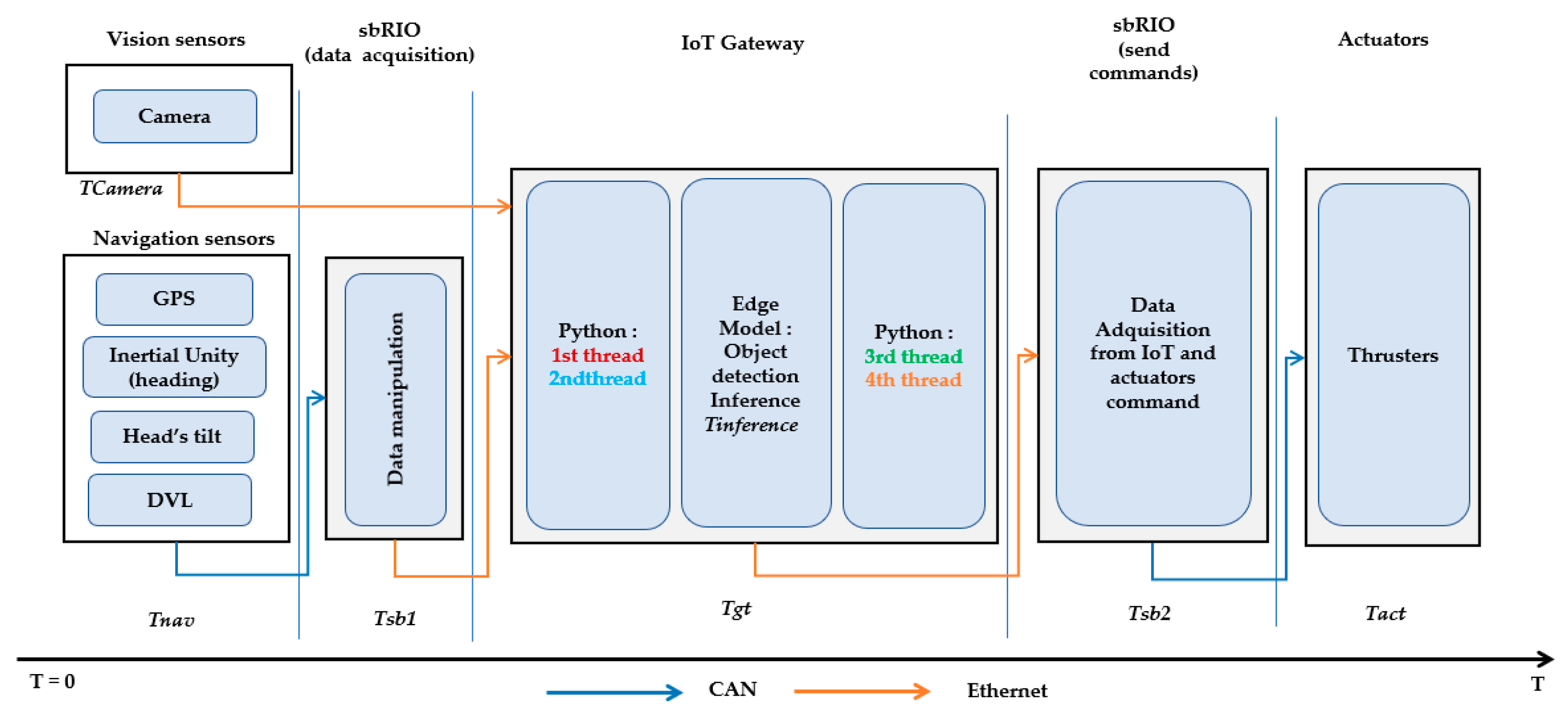
6.1.2. Edge Architecture

In the edge architecture, the data remains in the local machine and the images are not sent to the cloud; however, the application needs a minimal connection to the cloud to report usage, which is suitable for intermittent connectivity. The cloud connection is almost negligible; instead of sending photos to the cloud for processing, the model uploads to the local IoT gateway and performs the treatment. We therefore neglect the cloud connection in this architecture and only consider the connections in the AUV.
In the edge model deployed in the IoT gateway, the overall response time of the edge architecture in the AUV over the Ethernet and CAN networks is modelled as:
T = T s e n s + T s b 1 + T g t + T s b 2 + T a c t
where Tsens is expressed as:
T s e n s = { T n a v + T s b 1   if   T n a v + T s b 1 > T c a m e r a T c a m e r a   if   T n a v + T s b 1 < T c a m e r a  
Tgt, in this case, depends on Tthreads executing the four threads in the IoT gateway and the custom model Tinference uploaded from the cloud.
T g t = T t h r e a d s + T i n f e r e n c e  

6.2. Metrics

The Azure Custom Vision, Google cloud and Watson IBM services allow users to load a set of image data and define the bounding box of each desired object in the image. To train the model effectively, the images must be varied and as close as possible to the data on which the predictions will be made. Camera angle, blurring, background, lighting, size, low resolution and type are all important variations of the image that affect the training process.
Once the training was completed, we calculated the model’s performance using new image datasets (i.e., not included in the training dataset), shown in Table 1. Precision indicates the fraction of identified classifications that are correct, while recall indicates the fraction of actual classifications that are correctly identified. IoU (intersection over union) is a metric of how successfully a model predicts the objects’ locations and is gauged using the area of overlapping regions of the predicted and ground truth bounding boxes, defined as:
I o U = A r e a   o f   O v e r l a p A r e a   o f   U n i o n
Unlike IBM in Azure Custom Vision and Google cloud, the AI model can be exported in different formats (TensorFlow, Docker) specially adapted to edge devices, as opposed to in the cloud. The model trained for cloud use is different from that trained for the edge as regards accuracy and response time. We used the same photos to train and test the trained models for both edge and cloud use in the trials. Figure 15 shows some differences in terms of the accuracy of new photos not used in the training phase. The five tests clearly show the limits of each example; for instance, in test 3, the picture was blurred, and Google cloud could not detect the mussel, while Microsoft detected it with 83% accuracy and IBM only 15% accuracy. In test 2, all three clouds detected an unknown red object stuck in the sub-bottom as a mussel with different percentages, which shows the limitation of the models regarding colour changes.
In order to evaluate the performance of the proposed object detection models, in both the cloud and edge, we used the following standard performance metrics:
precision = T P F P + T P  
recall   = T P F N + T P  
where precision indicates the fraction of identified detections that were correct and recall indicates the fraction of actual detections that were correctly identified. FP (False Positive) represents the number of negative samples judged to be positive, TP (True Positive) is the number of positive samples judged to be positive, and FN (False Negative) is the number of positive samples judged to be negative.
The accuracy measurement tests were performed on all three cloud platforms. We also adopted the Azure edge model as it shows a better IoU metric score than Google. The accuracy test was performed on more than thirty photos of mussels detected by our AUV camera, using the same photos in the three different clouds. The results given in Table 1 clearly show the difference between the AI cloud services.

6.3. Latency Evaluation

Since most of the cloud APIs are based on the HTTP protocol, we performed a total of 100 HTTP throughput tests using SpeedTest between the web server and the IoT gateway installed in the AUV. The tests were performed in the Mar Menor experimental area through the 4G connection. The average results of the tests carried out in this experimental area were as follows: round trip delay: 66 ms; download: 16.6 Mbps; upload: 19.3 Mbps. The average size of the image sent from the AUV to the cloud was approximately 194 kb.
The local network which connects the vehicle and the buoy presents a low fixed latency. This was measured by a 100-automated-delay measurement campaign. The average latencies between the IoT gateway and the different devices in the vehicle’s Ethernet network were as follows: sbRIO: 0.9 ms; camera: 1.1 ms; 4G router (buoy): 1.2 ms.
The latency results are summarized in Table 2, where average, minimum and maximum response time values are calculated for each endpoint architecture. The experimental set-up was based on Azure and IBM cloud architectures, plus another edge architecture using a custom model formed by Azure and processed by the IoT gateway. Although IBM Watson and Azure custom vision are available worldwide, the locations of the deployments differ; Watson is deployed in the U.S. and South Korea [109], while Google cloud and Azure are deployed in various locations around the world [98,99]. In this case, the Azure and Google cloud services are deployed in Western Europe, while IBM is in Dallas, USA. All the samples in each architecture were thoroughly verified in an experimental campaign with over 100 valid samples. The experiments carried out were based on Equations (10) and (12) and Python software. The latter was employed to measure the overall latency.
The results reported in Table 2 show the differences between the proposed architectures in terms of latency. Despite the fact that image processing in edge computing is performed on the IoT gateway, the total response time is significantly lower than the latency obtained with cloud computing. The faster running time of the custom AI detection model ensures real-time tracking and navigation adjustment. Edge average response time is almost three times less than that of the cloud. However, the edge model is less accurate than the cloud model; in fact, the edge model loaded from the cloud is optimized as far as possible to meet the requirements of tiny device platforms.

7. Exploration Case Study

The experimental exploration mission was carried out with the objective of determining the viability of the previously described approaches in detecting fan mussel specimens in an area of 250 m × 100 m in the Mar Menor (with the coordinates of Table 3). A cloud architecture approach (Figure 12a) and a hybrid approach, a combination of cloud architecture (main mission) and edge architecture (tracking mission) were adopted (Figure 12b). The aim of the hybrid approach was to take advantage of edge architecture’s lower latency and favourable cloud precision. The tests achieved in the previous section lead us to conclude that the results of Azure custom vision are more pertinent to our use case application (in terms of latency and accuracy); therefore, we decided to adopt both the cloud and edge Azure models for the mission described below.
Our sailing operation started in a vessel equipped with a robotic arm that placed the vehicle in the water. After defining the coordinates of the inspection area, the mission was planned on IUNO software (Figure 16) according to the weather forecast, the time available and the width of the vehicle’s search path.
The AUV employed for the experiment was connected to the buoy as shown in Figure 17. The control station on board the vessel was connected to the AUV by 4G communications. The different systems were checked before the AUV was placed in the water: control, lighting, thrusters, 4G communications, vision, etc. After successfully validating the systems, the vehicle was launched and the mission was transferred from IUNO to the AUV.
We initiated the main mission using the first approach (cloud architecture for detection and tracking). The AUV started to explore the area for possible specimens. The average depth of the inspection area was 5.02 m and the vehicle remained at an average height of 2.01 m above the seabed.
The first of the six sweeps (Figure 16) was completed without detecting any possible specimens. The first fan mussel was detected with 63% accuracy in the second track, when the AUV switched to the secondary mission mode to track it (object location in the frame and distance calculation). However, this turned out to be quite impractical due to the high latency of the cloud connection. A timeout exception occurred during the tracking mission and the algorithm chose to ignore it and resume the main mission. As described in Section 6, the detection fails if a deadline is missed due to transmission delays, which affects the dynamic stability of the control system. The technical team therefore decided to abort the mission, return to the starting point and launch the same mission in the “hybrid” mode.
The hybrid mission mode was initiated and the cloud connection was used to process the photos sent during the main tracking mission. On the second sweep, the cloud results in the gateway indicated the presence of a specimen with 64% probability. The vehicle switched to the tracking mode. At this point, the AUV began manoeuvring to place the target in the centre of the image, while the inference was switched to the edge model in the IoT gateway instead of the cloud to reduce latency. The AUV was able to follow the suspected specimen up to a distance of 2.13 m. The accuracy of the analysed image at this distance was 83.8%, using the trained edge model. For greater certainty, the inference was switched to the cloud for the last picture to confirm the find. In this hybrid mode, the edge was used to speed up tracking and AUV response. At this point, the AUV ended the secondary mission mode, registered the find as positive, saved its coordinates and resumed the main mission (Figure 18).
No further specimens were detected until the fourth sweep, when another was detected with 38% probability. Once again, the vehicle switched to tracking mode, centred the target in the image and performed the approach manoeuvre as before. After halting at 2.06 m from the target, the recognition algorithm indicated that the target was a fan mussel with 59% probability. As the minimum confirmation requirement in terms of the probable detection threshold at this stage is 80%, the target was ignored, and the main mission was resumed. Due to the real-time communications, the target was in fact found not to be a fan mussel but a dark-coloured rock. On the sixth sweep, the mission and inspection were completed after detecting one target specimen and discarding another possible detection that turned out to be a rock.

8. Conclusions

This paper proposes an AUV model system designed to track a species of Mediterranean fan mussel, using cloud computing services with edge computing as alternative processing units. Edge computing topology reduces latency to support IoT performance in low-bandwidth environments and eases overall network congestion. An innovative algorithm was proposed to autonomously track the target species without human intervention by integrating the object detection system into the AUV control loop. The proposed model is capable of detecting, tracking and georeferencing specimens with IUNO software.
The obtained results highlight the system’s effectiveness and feature the asset of combining an AUV with deep learning cloud services for processing and analysing photos. Although cloud-based architecture automatically distributes and balances processing loads, we overcame latency challenges in the tracking process by using edge computing in the IoT gateway. The IoT gateway installed in the AUV replaces the cloud processing unit by virtue of the interaction between the different AUV components. We integrated cloud-based ML services into the AUV system to achieve a completely autonomous pre-programmed search mission with relevant accuracy. Moreover, to ensure that data is transferred, processed and returned at speeds that meet the needs of the application, the two cloud object detection services were implemented and compared in terms of latency and accuracy. The obtained experimental results clearly justify the proposed hybrid cloud/edge architecture and highlight the combination of the system performances that ensure a real-time control loop for relevant latency and accuracy.
To meet the system’s requirements, lower latency and favourable cloud precision, our proposed AUV servo control ensures a trade-off between performance and stability. The hybrid cloud/edge architecture is therefore recommended to ensure a real-time control loop and achieve consistent results.

Author Contributions

M.S. carried out this research as part of his Ph.D. thesis, under the supervision of A.G.-G., M.A. and F.J.O.; conceptualization, software and investigation, J.C.M.-M. The study was a joint research project between the Abdelmalek Essaadi University (Morocco) and the Polytechnic University of Cartagena (Spain) within the Erasmus+ program. All authors have read and agreed to the published version of the manuscript.

Funding

This research was funded by Comunidad Autónoma de la Región de Murcia (Consejería de Empresa, Industria y Portavocía) and cofunded by the Operative Program FEDER of the Murcia Region 2014-2020 in the Research and Innovation Strategies for Smart Specialisation RIS3MUR, grant project name: OBSERVATORIO OCEANOGRÁFICO MÓVIL DE LA REGIÓN DE MURCIA, Referencia: 2I18SAE00056.

Acknowledgments

The authors would like to thank the “Murcia Regional Research Program for Groups of Scientific Excellence” of the Seneca Foundation (Murcia Regional Agency for Science and Technology—19895/GERM/15).

Conflicts of Interest

The authors have no conflict of interest to declare.

References

  1. González-Reolid, I.; Molina-Molina, J.C.; Guerrero-González, A.; Ortiz, F.J.; Alonso, D. An Autonomous Solar-Powered Marine Robotic Observatory for Permanent Monitoring of Large Areas of Shallow Water. Sensors 2018, 18, 3497. [Google Scholar] [CrossRef] [PubMed] [Green Version]
  2. Boletín Oficial de la Región de Murcia, Numero 298, Viernes, 27 de Diciembre de 2019, Página 36008, 8089 Decreto-Ley N° 2/2019, de 26 de Diciembre, de Protección Integral del Mar Menor. Available online: https://www.borm.es/services/anuncio/ano/2019/numero/8089/pdf?id=782206 (accessed on 18 June 2020).
  3. Informe Integral Sobre el Estado Ecológico del Mar Menor; Comité de Asesoramiento Científico del Mar Menor: Murcia, Spain, 2017.
  4. Kersting, D.; Benabdi, M.; Čižmek, H.; Grau, A.; Jimenez, C.; Katsanevakis, S.; Öztürk, B.; Tuncer, S.; Tunesi, L.; Vázquez-Luis, M.; et al. Pinna nobilis. IUCN Red List Threat. Species 2019, e.T160075998A160081499. Available online: https://www.iucnredlist.org/species/160075998/160081499 (accessed on 19 June 2020). [CrossRef]
  5. del Año, M. La Nacra Pinna nobilis. In Noticiario de la Sociedad Española de Malacologia N° 67-2017; Moreno, D., Rolan, E., Troncoso, J.S., Eds.; Katsumi-san Co.: Cambridge, MA, USA, 2017. [Google Scholar]
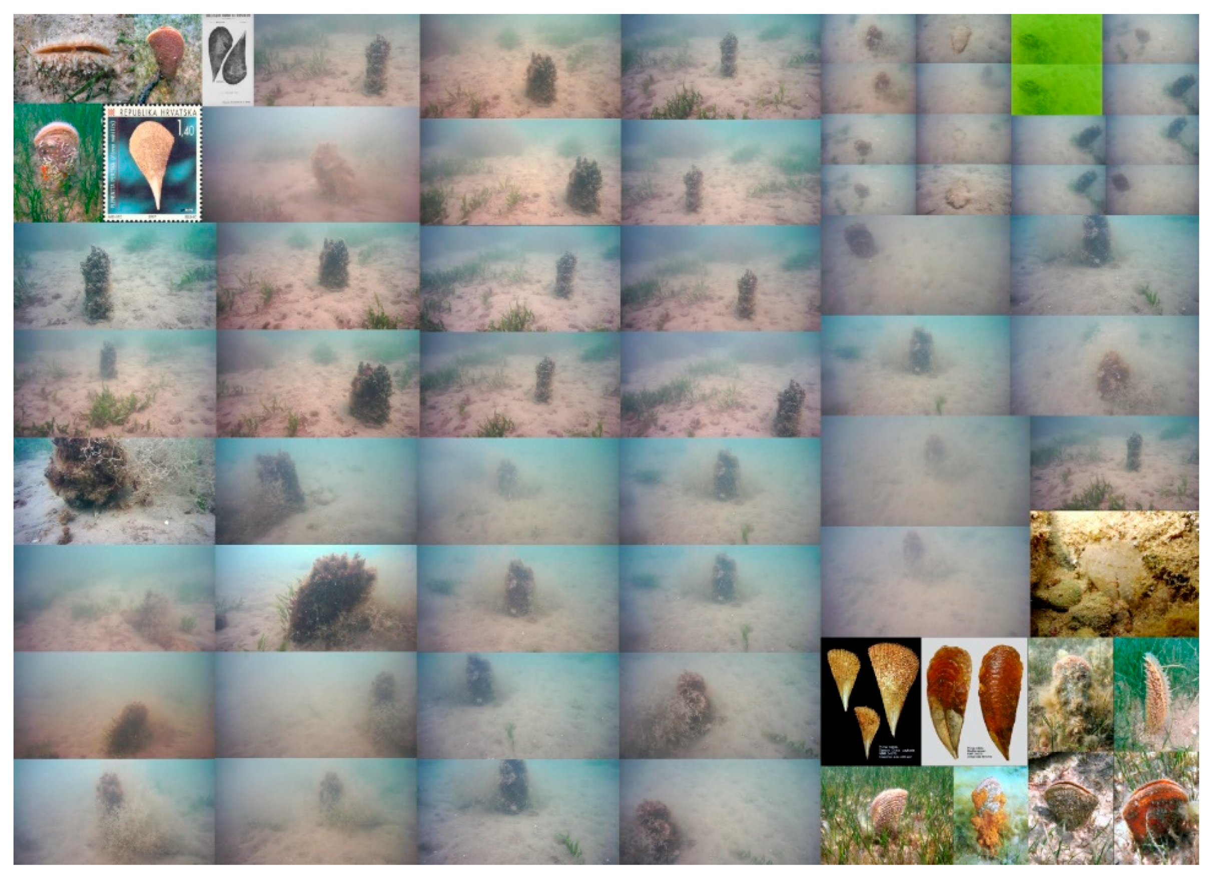
  6. Belando, M.D.; García-Muñoz, M.R.; Ramos-Segura, A.; Franco-Navarro, I.J.; García-Moreno, P.; Ruiz-Fernández, J.M. Distribución y Abundancia de las Praderas de MACRÓFITOS bentónicos y las Poblaciones de Nacra (Pinna nobilis) en el Mar Menor; Informe del Instituto Español de Oceanografía y la Asociación de Naturalistas del Sureste: Murcia, Spain, 2014; 60p. [Google Scholar]
  7. Paull, L.; Seto, M.; Saeedi, S.; Leonard, J.J. Navigation for Underwater Vehicles; Springer: Berlin/Heidelberg, Germany, 2018. [Google Scholar] [CrossRef]
  8. Liu, X.; Xu, X.; Liu, Y.; Wang, L. Kalman filter for cross-noise in the integration of SINS and DVL. Math. Probl. Eng. 2014, 2014, 1–8. [Google Scholar] [CrossRef]
  9. Paull, L.; Saeedi, S.; Seto, M.; Li, H. AUV navigation and localization: A review. IEEE J. Ocean. Eng. 2014, 39, 131–149. [Google Scholar] [CrossRef]
  10. Moysiadis, V.; Sarigiannidis, P.; Moscholios, I. Towards Distributed Data Management in Fog Computing. Wirel. Commun. Mob. Comput. 2018, 2018. [Google Scholar] [CrossRef]
  11. Armbrust, M.; Fox, A.; Griffith, R.; Joseph, A.D.; Katz, R.; Konwinski, A.; Lee, G.; Patterson, D.; Rabkin, A.; Stoica, I.; et al. A view of cloud computing. Commun. ACM 2010, 53, 50–58. [Google Scholar] [CrossRef] [Green Version]
  12. Kenitar, S.B.; Arioua, M.; Younes, A.; Radi, M.; Salhaoui, M. Comparative Analysis of Energy Efficiency and Latency of Fog and Cloud Architectures. In Proceedings of the 2019 International Conference on Sensing and Instrumentation in IoT Era (ISSI), Lisbon, Portugal, 29–30 August 2019; IEEE: Piscataway, NJ, USA, 2020. [Google Scholar] [CrossRef]
  13. Redmon, J.; Divvala, S.; Girshick, R.; Farhadi, A. You only look once: Unified, real-time object detection. In Proceedings of the IEEE Conference on Computer Vision and Pattern Recognition (CVPR 2016), Las Vegas, NV, USA, 27–30 June 2016; pp. 779–788. [Google Scholar]
  14. Wang, X.; Victor, C.M.; Niyato, D.; Yan, X.; Chen, X. Convergence of Edge Computing and Deep Learning: A Comprehensive Survey. IEEE Commun. Surv. Tutor. 2020, 22, 869–904. [Google Scholar] [CrossRef] [Green Version]
  15. Computer Vision, WikiPedia. Available online: https://en.wikipedia.org/wiki/Computer_vision (accessed on 18 June 2020).
  16. Feng, X.; Jiang, Y.; Yang, X.; Du, M.; Li, X. Computer Vision Algorithms and Hardware Implementations: A Survey. Integration 2019, 69, 309–320. [Google Scholar] [CrossRef]
  17. Kang, Y.; Hauswald, J.; Gao, C.; Rovinski, A.; Mudge, T.; Mars, J.; Tang, L. Neurosurgeon: Collaborative Intelligence Between the Cloud and Mobile Edge. In Proceedings of the 22nd International Conference on Architectural Support for Programming Languages and Operating Systems (ASPLOS 2017), Xi’an, China, 8–12 April 2017; pp. 615–629. [Google Scholar]
  18. Basagni, S.; Conti, M.; Giordano, S.; Stojmenovic, I. Advances in Underwater Acoustic Networking. In Mobile Ad Hoc Networking: The Cutting Edge Directions; IEEE: Piscataway, NJ, USA, 2013; pp. 804–852. [Google Scholar]
  19. Luo, H.; Wu, K.; Ruby, R.; Liang, Y.; Guo, Z.; Ni, L.M. Software-Defined Architectures and Technologies for Underwater Wireless Sensor Networks: A Survey. IEEE Commun. Surv. Tutor. 2018, 20, 2855–2888. [Google Scholar] [CrossRef]
  20. Dol, H.S.; Casari, P.; van der Zwan, T.; Otnes, R. Software-Defined Underwater Acoustic Modems: Historical Review and the NILUS Approach. IEEE J. Ocean. Eng. 2017, 42, 722–737. [Google Scholar] [CrossRef]
  21. Xu, G.; Shi, Y.; Sun, X.; Shen, W. Internet of Things in Marine Environment Monitoring: A Review. Sensors 2019, 19, 1711. [Google Scholar] [CrossRef] [PubMed] [Green Version]
  22. Bao, J.; Li, D.; Qiao, X.; Rauschenbach, T. Integrated navigation for autonomous underwat vehicles in aquaculture: A review. Inf. Process. Agric. 2020, 7, 139–151. [Google Scholar] [CrossRef]
  23. Generation and Processing of Simulated Underwater Images for Infrastructure Visual Inspection with UUVs. Sensors 2019, 19, 5497. [CrossRef] [PubMed] [Green Version]
  24. Wynn, R.B.; Huvenne, V.A.I.; le Bas, T.P.; Murton, B.; Connelly, D.P.; Bett, B.J.; Ruhl, H.A.; Morris, K.J.; Peakall, J.; Parsons, D.R.; et al. Autonomous Underwater Vehicles (AUVs): Their past, present and future contributions to the advancement of marine geoscience. Mar. Geol. 2014. [Google Scholar] [CrossRef] [Green Version]
  25. Barrett, N.; Seiler, J.; Anderson, T.; Williams, S.; Nichol, S.; Hill, N. Autonomous Underwater Vehicle (AUV) for mapping marine biodiversity in coastal and shelf waters: Implications for Marine Management. In Proceedings of the OCEANS’10 IEEE Conference, Sydney, Australia, 24−27 May 2010. [Google Scholar]
  26. Liu, S.; Xu, H.; Lin, Y.; Gao, L. Visual Navigation for Recovering an AUV by Another AUV in Shallow Water. Sensors 2019, 19, 1889. [Google Scholar] [CrossRef] [Green Version]
  27. Corgnati, L.; Marini, S.; Mazzei, L.; Ottaviani, E.; Aliani, S.; Conversi, A.; Griffa, A. Looking inside the Ocean: Toward an Autonomous Imaging System for Monitoring Gelatinous Zooplankton. Sensors 2016, 16, 2124. [Google Scholar] [CrossRef] [Green Version]
  28. Yoerger, D.R.; Bradley, A.M.; Walden, B.B.; Singh, H.; Bachmayer, R. Surveying asubsea lavaflow using the Autonomous Benthic Explorer (ABE). Int. J. Syst. Sci. 1998, 10, 1031–1044. [Google Scholar] [CrossRef]
  29. Yoerger, D.R.; Bradley, A.M.; Jakuba, M.; German, C.R.; Shank, T.; Tivey, M. Autono-mous and remotely operated vehicle technology for hydrothermal vent discovery, exploration, and sampling. Oceanography 2007, 20, 152–161. [Google Scholar] [CrossRef] [Green Version]
  30. Caress, D.W.; Thomas, H.; Kirkwood, W.J.; McEwen, R.; Henthorn, R.; Clague, D.A.; Paull, C.K.; Paduan, J. High-Resolution Multibeam, Sides Can and Sub Bottomsurveys Using the MBARI AUVD; Allan, B., Greene, H.G., Reynolds, J.R., Eds.; Marine HabitatMapping Technology for Alaska, Alaska Sea Grant College Program; University of Alaska: Fairbanks, Alaska, 2008; pp. 47–69. [Google Scholar]
  31. Silva, E.; Martins, A.; Dias, A.; Matos, A.; Olivier, A.; Pinho, C.; Silva, E.; de Sá, F.A.; Ferreira, H.; Silva, H.; et al. Strengthening marine and maritime research and technology. In Proceedings of the OCEANS 2016 MTS/IEEE Monterey, Monterey, CA, USA, 19–23 September 2016; pp. 1–9. [Google Scholar]
  32. Nicholson, J.; Healey, A. The present state of autonomous underwater vehicle (AUV) applications and technologies. Mar. Technol. Soc. J. 2008, 42, 44–51. [Google Scholar] [CrossRef]
  33. Lucieer, V.L.; Forrest, A.L. Emerging Mapping Techniques for Autonomous Underwater Vehicles (AUVs). In Seafloor Mapping along Continental Shelves: Research and Techniques for Visualizing Benthic Environments; Finkl, C.W., Makowski, C., Eds.; Springer International Publishing: Cham, Switzerland, 2016. [Google Scholar]
  34. Wynn, R.; Bett, B.; Evans, A.; Griffiths, G.; Huvenne, V.; Jones, A.; Palmer, M.; Dove, D.; Howe, J.; Boyd, T. Investigating the Feasibility of Utilizing AUV and Glider 33 Technology for Mapping and Monitoring of the UK MPA Network; National Oceanography Centre: Southampton, UK, 2012. [Google Scholar]
  35. Weidner, N.; Rahman, S.; Li, A.Q.; Rekleitis, I. Underwater cave mapping using stereo vision. In Proceedings of the IEEE International Conference on Robotics and Automation, Singapore, 29 May–3 June 2017; pp. 5709–5715. [Google Scholar]
  36. Hernández, J.D.; Istenic, K.; Gracias, N.; García, R.; Ridao, P.; Carreras, M. Autonomous seabed inspection for environmental monitoring. In Advances in Intelligent Systems and Computing, Proceedings of the Robot 2015: Second Iberian Robotics Conference, Lisbon, Portugal, 19–21 November 2015; Springer: Berlin, Germany, 2016; pp. 27–39. [Google Scholar]
  37. Johnson-Roberson, M.; Bryson, M.; Friedman, A.; Pizarro, O.; Troni, G.; Ozog, P.; Henderson, J.C. High-resolution underwater robotic vision-based mapping and three-dimensional reconstruction for archaeology. J. Field Robot. 2017, 34, 625–643. [Google Scholar] [CrossRef] [Green Version]
  38. Ozog, P.; Carlevaris-Bianco, N.; Kim, A.; Eustice, R.M. Long-term Mapping Techniques for Ship Hull Inspection and Surveillance using an Autonomous Underwater Vehicle. J. Field Robot. 2016, 33, 265–289. [Google Scholar] [CrossRef] [Green Version]
  39. Bonnin-Pascual, F.; Ortiz, A. On the use of robots and vision technologies for the inspection of vessels: A survey on recent advances. Ocean. Eng. 2019, 190, 106420. [Google Scholar] [CrossRef]
  40. Plymouth University. Available online: https://www.plymouth.ac.uk/news/study-explores-the-use-of-robots-and-artificial-intelligence-to-understand-the-deep-sea (accessed on 12 July 2019).
  41. High, R.; Bakshi, T. Cognitive Computing with IBM Watson: Build Smart Applications Using Artificial Intelligence as a Service; Published by Packt Publishing: Birmingham, UK, 2019. [Google Scholar]
  42. Lu, H.; Li, Y.; Zhang, Y.; Chen, M.; Serikawa, S.; Kim, H. Underwater Optical Image Processing: A Comprehensive Review. arXiv 2017, arXiv:1702.03600. [Google Scholar] [CrossRef]
  43. Schechner, Y.; Averbuch, Y. Regularized image recovery in scattering media. IEEE Trans. Pattern Anal. Mach. Intell. 2007, 29, 1655–1660. [Google Scholar] [CrossRef] [PubMed] [Green Version]
  44. Yemelyanov, K.; Lin, S.; Pugh, E.; Engheta, N. Adaptive algorithms for two-channel polarization sensing under various polarization statistics with nonuniform distributions. Appl. Opt. 2006, 45, 5504–5520. [Google Scholar] [CrossRef]
  45. Arnold-Bos, A.; Malkasset, J.; Kervern, G. Towards a model-free denoising of underwater optical images. In Proceedings of the IEEE Europe Oceans Conference, Brest, France, 20–23 June 2005; pp. 527–532. [Google Scholar]
  46. Roser, M.; Dunbabin, M.; Geiger, A. Simultaneous underwater visibility assessment, enhancement and improved stereo. In Proceedings of the IEEE International Conference on Robotics and Automation, Hong Kong, China, 31 May–7 June 2014; pp. 1–8. [Google Scholar]
  47. Lu, H.; Li, Y.; Xu, X.; He, L.; Dansereau, D.; Serikawa, S. Underwater image descattering and quality assessment. In Proceedings of the IEEE International Conference on Image Processing, Phoenix, AZ, USA, 25–28 September 2016; pp. 1998–2002. [Google Scholar]
  48. Lu, H.; Serikawa, S. Underwater scene enhancement using weighted guided median filter. In Proceedings of the IEEE International Conference on Multimedia and Expo, Chengdu, China, 14–18 July 2014; pp. 1–6. [Google Scholar]
  49. Foresti, G.L.; Murino, V.; Regazzoni, C.S.; Trucco, A. A Voting-Based Approach for Fast Object Recognition in Underwater Acoustic Images. IEEE J. Ocean. Eng. 1997, 22, 57–65. [Google Scholar] [CrossRef]
  50. Hansen, R.K.; Andersen, P.A. 3D Acoustic Camera for Underwater Imaging. Acoust. Imaging 1993, 20, 723–727. [Google Scholar]
  51. Lane, D.M.; Stoner, J.P. Automatic interpretation of sonar imagery using qualitative feature matching. IEEE J. Ocean. Eng. 1994, 19, 391–405. [Google Scholar] [CrossRef]
  52. Wang, Y.; Zhang, J.; Cao, Y.; Wang, Z. A deep CNN method for underwater image enhancement. In Proceedings of the IEEE International Conference on Image Processing (ICIP), Beijing, China, 17–20 September 2017; pp. 1382–1386. [Google Scholar]
  53. Li, J.; Skinner, K.A.; Eustice, R.M.; Johnson-Roberson, M. WaterGAN: Unsupervised generative network to enable real-time color correction of monocular underwater images. IEEE Robot. Autom. Lett. 2017, 3, 387–394. [Google Scholar] [CrossRef] [Green Version]
  54. Oleari, F.; Kallasi, F.; Rizzini, D.L.; Aleotti, J.; Caselli, S. An underwater stereo vision system: From design to deployment and dataset acquisition. In Proceedings of the Oceans’15 MTS/IEEE, Genova, Italy, 18–21 May 2015; pp. 1–6. [Google Scholar]
  55. Sanz, P.J.; Ridao, P.; Oliver, G.; Melchiorri, C.; Casalino, G.; Silvestre, C.; Petillot, Y.; Turetta, A. TRIDENT: A framework for autonomous underwater intervention missions with dexterous manipulation capabilities. IFAC Proc. Vol. 2010, 43, 187–192. [Google Scholar] [CrossRef]
  56. Duarte, A.; Codevilla, F.; Gaya, J.D.O.; Botelho, S.S. A dataset to evaluate underwater image restoration methods. In Proceedings of the OCEANS, Shanghai, China, 10–13 April 2016; pp. 1–6. [Google Scholar]
  57. Ferrera, M.; Moras, J.; Trouvé-Peloux, P.; Creuze, V.; Dégez, D. The Aqualoc Dataset: Towards Real-Time Underwater Localization from a Visual-Inertial-Pressure Acquisition System. arXiv 2018, arXiv:1809.07076. [Google Scholar]
  58. Akkaynak, D.; Treibitz, T.; Shlesinger, T.; Loya, Y.; Tamir, R.; Iluz, D. What is the space of attenuation coefficients in underwater computer vision? In Proceedings of the IEEE Conference on Computer Vision and Pattern Recognition, Honolulu, HI, USA, 21–26 July 2017; pp. 4931–4940. [Google Scholar]
  59. Foresti, G.L.; Gentili, S. A Vison Based System for Object Detection In Underwater Images. Int. J. Pattern Recognit. Artif. Intell. 2000, 14, 167–188. [Google Scholar] [CrossRef]
  60. Valdenegro-Toro, M. Improving Sonar Image Patch Matching via Deep Learning. In Proceedings of the 2017 European Conference on Mobile Robots (ECMR), Paris, France, 6–8 September 2017. [Google Scholar] [CrossRef] [Green Version]
  61. Villon, S.; Mouillot, D.; Chaumont, M.; Darling, E.S.; Subsolb, G.; Claverie, T.; Villéger, S. A Deep Learning method for accurate and fast identification of coral reef fishes in underwater images. Ecol. Inform. 2018. [Google Scholar] [CrossRef] [Green Version]
  62. Rampasek, L.; Goldenberg, A. TensorFlow: Biology’s Gateway to Deep Learning. Cell Syst. 2016, 2, 12–14. [Google Scholar] [CrossRef] [PubMed] [Green Version]
  63. Weinstein, B.G. A computer vision for animal ecology. J. Anim. Ecol. 2018, 87, 533–545. [Google Scholar] [CrossRef]
  64. Gomes-Pereira, J.N.; Auger, V.; Beisiegel, K.; Benjamin, R.; Bergmann, M.; Bowden, D.; Buhl-Mortensen, P.; De Leo, F.C.; Dionísio, G.; Durden, J.M. Current and future trends in marine image annotation software. Prog. Oceanogr. 2016, 149, 106–120. [Google Scholar] [CrossRef]
  65. Qut University. Available online: https://www.qut.edu.au/news?id=135108 (accessed on 3 May 2020).
  66. Piechaud, N.; Hunt, C.; Culverhouse, P.F.; Foster, N.L.; Howell, K.L. Automated identification of benthic epifauna with computer vision. Mar. Ecol. Prog. Ser. 2019, 615, 15–30. [Google Scholar] [CrossRef]
  67. Lorencik, D.; Tarhanicova, M.; Sincak, P. Cloud-Based Object Recognition: A System Proposal; Springer International Publishing: Cham, Switzerland, 2014. [Google Scholar] [CrossRef]
  68. Embedded-Vision. Available online: https://www.embedded-vision.com/platinum-members/embedded-vision-alliance/embedded-vision-training/documents/pages/cloud-vs-edge (accessed on 3 May 2020).
  69. Wang, X.; Han, Y.; Leung, V.C.; Niyato, D.; Yan, X.; Chen, X. Convergence of Edge Computing and Deep Learning: A Comprehensive Survey. arXiv 2019, arXiv:1907.08349v2. [Google Scholar] [CrossRef] [Green Version]
  70. Kim, D.; Han, K.; Sim, J.S.; Noh, Y. Smombie Guardian: We watch for potentialobstacles while you are walking andconducting smartphone activities. PLoS ONE 2018, 13, e0197050. [Google Scholar] [CrossRef]
  71. Megalingam, R.K.; Shriram, V.; Likhith, B.; Rajesh, G.; Ghanta, S. Monocular distance estimation using pinhole camera approximation to avoid vehicle crash and back-over accidents. In Proceedings of the 2016 10th International Conference on Intelligent Systems and Control (ISCO), Coimbatore, India, 7–8 January 2016; IEEE: Coimbatore, India. [Google Scholar] [CrossRef]
  72. Salhaoui, M.; Guerrero-Gonzalez, A.; Arioua, M.; Ortiz, F.J.; El Oualkadi, A.; Torregrosa, C.L. Smart industrial iot monitoring and control system based on UAV and cloud computing applied to a concrete plant. Sensors 2019, 19, 3316. [Google Scholar] [CrossRef] [Green Version]
  73. Stackoverflow. Available online: https://stackoverflow.blog/2017/09/14/python-growing-quickly/ (accessed on 3 May 2020).
  74. Netguru. Available online: https://www.netguru.com/blog/why-is-python-good-for-research-benefits-of-the-programming-language (accessed on 3 May 2020).
  75. Zhou, Z.; Chen, X.; Li, E.; Zeng, L.; Luo, K.; Zhang, J. Edge Intelligence: Paving the Last Mile of Artificial Intelligence with Edge Computing. Proc. IEEE 2019, 107. [Google Scholar] [CrossRef] [Green Version]
  76. Sikeridis, D.; Papapanagiotou, I.; Rimal, B.P.; Devetsikiotis, M. A Comparative Taxonomy and Survey of Public Cloud Infrastructure Vendors. arXiv 2018, arXiv:1710.01476v2. [Google Scholar]
  77. National Instruments. Available online: https://www.ni.com/es-es/support/model.sbrio-9606.html (accessed on 3 May 2020).
  78. National Instruments. Available online: https://www.ni.com/en-us/shop/labview.html (accessed on 3 May 2020).
  79. Buttazzo Giorgio, C. Hard Real-Time Computing Systems: Predictable Scheduling Algorithms and Applications; Springer Science & Business Media: New York, NY, USA, 2011; Volume 24. [Google Scholar]
  80. Pathak, A.R.; Pandey, M.; Rautaray, S. Application of Deep Learning for Object Detection. In Proceedings of the International Conference on Computational Intelligence and Data Science (ICCIDS 2018), Gurugram, India, 7–8 April 2018. [Google Scholar]
  81. Zhao, Z.; Zheng, P.; Xu, S.; Wu, X. Object Detection with Deep Learning: A Review. IEEE Trans. Neural Netw. Learn. Syst. 2019, 30, 3212–3232. [Google Scholar] [CrossRef] [PubMed] [Green Version]
  82. Dahlkamp, H.; Kaehler, A.; Stavens, D.; Thrun, S.; Bradski, G.R. Self supervised monocular road detection in desert terrain. In Proceedings of the Robotics: Science and Systems, Philadelphia, PA, USA, 16–19 August 2006. [Google Scholar]
  83. Chen, C.; Seff, A.; Kornhauser, A.; Xiao, J. Deep Driving: Learning affordance for direct perception in autonomous driving. In Proceedings of the 2015 IEEE International Conference on Computer Vision (ICCV), Santiago, Chile, 7–13 December 2015; pp. 2722–2730. [Google Scholar]
  84. Chen, X.; Ma, H.; Wan, J.; Li, B.; Xia, T. Multi-view 3D object detection network for autonomous driving. In Proceedings of the 2017 IEEE International Conference on Computer Vision (ICCV), Honolulu, HI, USA, 21–26 July 2017; pp. 6526–6534. [Google Scholar]
  85. Coates, A.; Ng, A.Y. Multi-camera object detection for robotics. In Proceedings of the 2010 IEEE International Conference on Robotics and Automation, Anchorage, AK, USA, 3–7 May 2010; pp. 412–419. [Google Scholar]
  86. Donahue, J.; Hendricks, L.A.; Guadarrama, S.; Rohrbach, M.; Venugopalan, S.; Saenko, K.; Darrell, T. Long-term recurrent convolutional networks for visual recognition and description. In Proceedings of the IEEE Conference on Computer Vision and Pattern Recognition, Santiago, Chile, 7–13 December 2015; pp. 2625–2634. [Google Scholar]
  87. Zhiqiang, W.; Jun, L. A review of object detection based on convolutional neural network. In Proceedings of the 2017 36th Chinese Control Conference (CCC), Dalian, China, 26–28 July 2017. [Google Scholar] [CrossRef]
  88. Krizhevsky, A.; Sutskever, I.; Hinton, G.E. ImageNet classification with deep convolutional neural networks. In Proceedings of the International Conference on Neural Information Processing Systems, Lake Tahoe, NV, USA, 3–8 December 2012; pp. 1097–1105. [Google Scholar]
  89. Deng, J.; Dong, W.; Socher, R.; Li, L.J.; Li, K.; Li, F.F. ImageNet: A large-scale hierarchical image database. In Proceedings of the Computer Vision and Pattern Recognition, 2009 (CVPR 2009), Miami, FL, USA, 20–25 June 2009; pp. 248–255. [Google Scholar]
  90. Girshick, R. Fast R-CNN. In Proceedings of the 2015 IEEE International Conference on Computer Vision (ICCV), Santiago, Chile, 7–13 December 2015. [Google Scholar] [CrossRef]
  91. Ren, S.; He, K.; Girshick, R.; Sun, J. Faster R-CNN: Towards Real-Time Object Detection with Region Proposal Networks. IEEE Trans. Pattern Anal. Mach. Intell. 2017, 39, 1137–1149. [Google Scholar] [CrossRef] [Green Version]
  92. Lin, T.; Goyal, P.; Girshick, R.; He, K.; Dollár, P. Focal Loss for Dense Object Detection. In Proceedings of the 2017 IEEE International Conference on Computer Vision (ICCV), Honolulu, HI, USA, 21–26 July 2017. [Google Scholar] [CrossRef] [Green Version]
  93. Liu, W.; Anguelov, D.; Erhan, D.; Szegedy, C.; Reed, S.; Fu, C.Y.; Berg, A.C. SSD: Single shot multibox detector. In Proceedings of the European Conference on Computer Vision, Amsterdam, The Netherlands, 11–14 October 2016; pp. 21–37. [Google Scholar]
  94. Ghidoni, P.L.N.S.; Brahnam, S. Handcrafted vs. non-handcrafted features for computer vision classification. Pattern Recognit. 2017, 71, 158–172. [Google Scholar] [CrossRef]
  95. Marine Species. Available online: http://www.marinespecies.org/ (accessed on 2 June 2020).
  96. Shi, W.; Cao, J.; Zhang, Q.; Li, Y.; Xu, L. Edge computing: Vision and challenges. IEEE Internet Things J. 2016, 3, 637–646. [Google Scholar] [CrossRef]
  97. Mao, Y.; You, C.; Zhang, J.; Huang, K.; Letaief, K.B. A survey on mobile edge computing: The communication perspective. IEEE Commun. Surv. Tutor. 2017, 19, 2322–2358. [Google Scholar] [CrossRef] [Green Version]
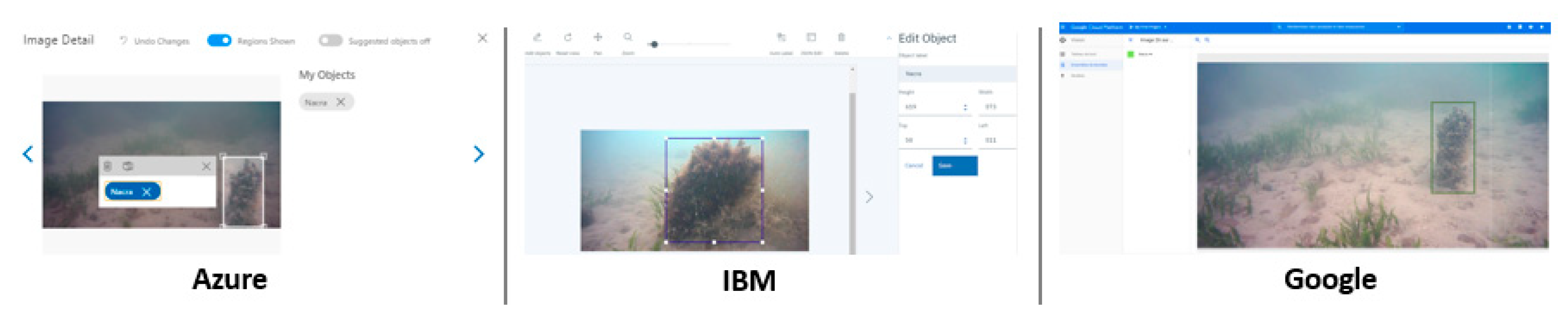
  98. Google Cloud. Available online: https://cloud.google.com/vision/?hl=en (accessed on 3 May 2020).
  99. Azure. Available online: https://azure.microsoft.com/en-au/services/cognitive-services/computer-vision/ (accessed on 3 May 2020).
  100. Chaumette, F.; Hutchinson, S. Visual servo control, Part I: Basic approaches. IEEE Robot. Autom. Mag. 2006, 13. [Google Scholar] [CrossRef]
  101. Prats, M.; Palomeras, N.; Ridao, P.; Sanz, P.J. Template Tracking and Visual Servoing for Alignment Tasks with Autonomous Underwater Vehicles. In Proceedings of the 9th IFAC Conference on Manoeuvring and Control of Marine Craft, Arenzano, Italy, 19–21 September 2012. [Google Scholar]
  102. Gao, J.; Liu, C.; Proctor, A. Nonlinear model predictive dynamic positioning control of an underwater vehicle with an onboard USBL system. J. Mar. Sci. Technol. 2016, 21, 57–69. [Google Scholar] [CrossRef]
  103. Krupinski, S.; Desouche, R.; Palomeras, N.; Allibert, G.; Hua, M.D. Pool Testing of AUV Visual Servoing for Autonomous Inspection. IFAC-PapersOnLine 2015, 48, 274–280. [Google Scholar] [CrossRef]
  104. Kumar, G.S.; Unnikrishnan, V.; Painumgal, M.N.V.; Kumar, C.; Rajesh, K.H.V. Autonomous Underwater Vehicle for Vision Based Tracking. Procedia Comput. Sci. 2018. [Google Scholar] [CrossRef]
  105. Islam, M.J.; Fulton, M.; Sattar, J. Towards a Generic Diver-Following Algorithm: Balancing Robustness and Efficiency in Deep Visual Detection. IEEE Robot. Autom. Lett. 2019, 4, 113–120. [Google Scholar] [CrossRef] [Green Version]
  106. Yosafat, R.; Machbub, C.; Hidayat, E.M.I. Design and Implementation of Pan-Tilt for Face Tracking. In Proceedings of the International Conference on System Engineering and Technology, Shah Alam, Malaysia, 2–3 October 2017. [Google Scholar]
  107. Zhang, B.; Huang, J.; Lin, J. A Novel Algorithm for Object Tracking by Controlling PAN/TILT Automatically. In Proceedings of the ICETC 2nd International Conference on Intelligent System 2010, Shanghai, China, 22–24 June 2010; Volume VI, pp. 596–602. [Google Scholar]
  108. González, A.G.; Coronado, J. Tratamiento de los retrasos del procesamiento visual en el sistema de control de un cabezal estereoscópico. In XX Jornadas de Automática: Salamanca, 27, 28 y 29 de Septiembre; Universidad de Salamanca: Salamanca, Spain; pp. 83–87.
  109. IBM. Available online: https://cloud.ibm.com/docs/services/visual-recognition?topic=visual-recognition-object-detection-overview (accessed on 3 May 2020).
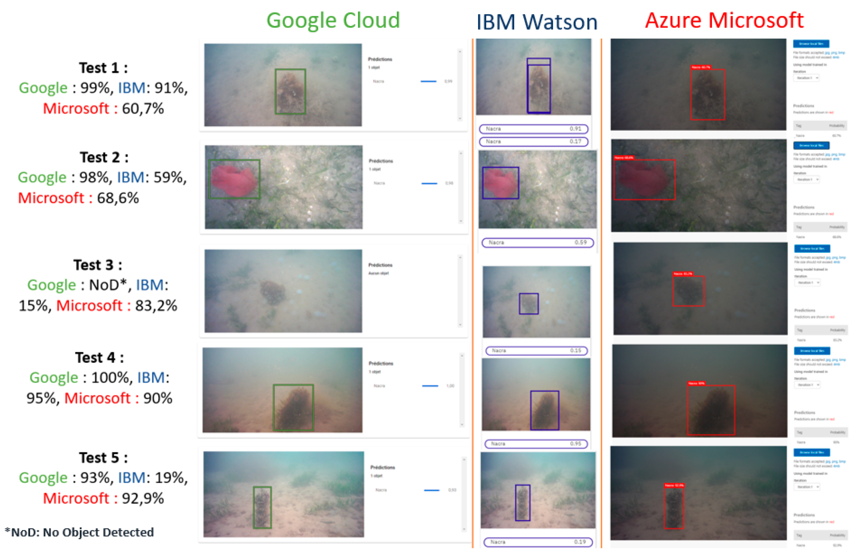
Figure 1. Proposed AUV-IoT Platform.
Remotesensing 12 01981 g001
Figure 2. Proposed hardware architecture.
Remotesensing 12 01981 g002
Figure 3. Communication between platforms.
Remotesensing 12 01981 g003
Figure 4. Node intercommunications and concurrent threads in the IoT gateway.
Remotesensing 12 01981 g004
Figure 5. Fan mussel recognition training: defining a fan mussel bounding box in different cloud services.
Remotesensing 12 01981 g005
Figure 6. Pictures used for custom CV model training.
Remotesensing 12 01981 g006
Figure 7. New specimen detection using the IBM Python API.
Remotesensing 12 01981 g007
Figure 8. Six-level rating for edge intelligence [75].
Remotesensing 12 01981 g008
Figure 9. Triangular similarity using a single camera [69].
Remotesensing 12 01981 g009
Figure 10. Closed control loop for object detection and tracking.
Remotesensing 12 01981 g010
Figure 11. Basic closed-loop system with sensor and actuator delays.
Remotesensing 12 01981 g011
Figure 12. Communication edge cloud. (a) Training and inference in the cloud; (b) training in the cloud, inference in the edge.
Remotesensing 12 01981 g012
Figure 13. Latency in the proposed platform within the cloud architecture.
Remotesensing 12 01981 g013
Figure 14. Edge architecture latency in the proposed platform.
Remotesensing 12 01981 g014
Figure 15. Cloud-based custom models for detecting new specimens.
Remotesensing 12 01981 g015
Figure 16. Mission generated in IUNO and uploaded into AUV.
Remotesensing 12 01981 g016
Figure 17. Deploying the platform to initiate the mission. AUV submarine connected to a buoy via a DSL cable.
Remotesensing 12 01981 g017
Figure 18. Specimen detection and positioning in IUNO.
Remotesensing 12 01981 g018
Table 1. Accuracy measurement in different platforms.
TPFPFNPrecisionRecallIoU
IBM28280.9333330.7777780.82506
Google223130.9166660.6111110.83364
Azure cloud33430.8918920.9166670.86601
Azure edge243110.8888890.6666670.678634
Table 2. Latency measurement in different platforms.
Total Response Time (ms)Cloud Response Time (ms)IoT Computing Time (ms)Capturing and Writing Time (ms)
MinMaxMeanMinMaxMeanMinMaxMeanMinMaxMean
IBM14074060206412803896193500093192129
Google12914384169611604071152000092196130
Azure12984572170311714435157100092196131
Azure edge62368763400052359553293194130
Table 3. GPS coordinates of the area explored.
CornerLatitudeLongitude
North east37.697635°−0.780121°
North west37.697635°−0.782876°
South west37.696825°−0.782876°
South east37.696825°−0.780121°

