Deep Learning for Land Cover Classification Using Only a Few Bands

Abstract

There is an emerging interest in using hyperspectral data for land cover classification. The motivation behind using hyperspectral data is the notion that increasing the number of narrowband spectral channels would provide richer spectral information and thus help improve the land cover classification performance. Although hyperspectral data with hundreds of channels provide detailed spectral signatures, the curse of dimensionality might lead to degradation in the land cover classification performance. Moreover, in some practical applications, hyperspectral data may not be available due to cost, data storage, or bandwidth issues, and RGB and near infrared (NIR) could be the only image bands available for land cover classification. Light detection and ranging (LiDAR) data is another type of data to assist land cover classification especially if the land covers of interest have different heights. In this paper, we examined the performance of two Convolutional Neural Network (CNN)-based deep learning algorithms for land cover classification using only four bands (RGB+NIR) and five bands (RGB+NIR+LiDAR), where these limited number of image bands were augmented using Extended Multi-attribute Profiles (EMAP). The deep learning algorithms were applied to a well-known dataset used in the 2013 IEEE Geoscience and Remote Sensing Society (GRSS) Data Fusion Contest. With EMAP augmentation, the two deep learning algorithms were observed to achieve better land cover classification performance using only four bands as compared to that using all 144 hyperspectral bands.

1. Introduction

Hyperspectral data have been used for chemical agent detection and classification [1,2], small target detection [3,4], fire damage assessment [5,6], anomaly detection [7,8,9,10,11,12,13], border monitoring [14], change detection [15,16,17,18], and mineral map abundance estimation on Mars [19,20]. Land cover classification is another application area where hyperspectral data are used extensively [21]. To improve land cover classification, the use of light detection and ranging (LiDAR) data and the fusion of LiDAR and hyperspectral data have been considered by several works [22,23,24,25,26,27]. Because some land covers differ among themselves with respect to their height, height could be a valuable piece of information.

There is also an increasing interest in adapting deep learning methods for land cover classification after several breakthroughs have been reported in a variety of computer vision tasks such as image classification, object detection and tracking, and semantic segmentation. The authors of [28] described an unsupervised feature extraction framework, with the name “patch-to-patch convolutional neural network (PToP CNN)”, which was used for land cover classification using hyperspectral and LiDAR data. The authors of [29] introduced a spectral-spatial attention network for image classification using hyperspectral data. In this network, while the recurrent neural network (RNN) part with attention can learn inner spectral correlations within a continuous spectrum, the CNN part is for the saliency features and aims to extract spatial relevance between neighboring pixels in the spatial dimension. The authors of [30] used convolutional networks for multispectral image classification. The authors of [31] provided a comprehensive review on land cover classification and object detection approaches using high-resolution imagery. The performances of deep learning models were evaluated against traditional approaches, and the authors concluded that the deep-learning-based methods provided an end-to-end solution and showed better performance than the traditional pixel-based methods by utilizing both spatial and spectral information, whereas traditional pixel-based methods resulted in salt-and-pepper-type noisy land cover map estimates. A number of other works have also shown that semantic segmentation classification with deep learning methods are quite promising in land cover classification [32,33,34,35].

Researchers also utilized spatial information in hyperspectral data via the use of Extended Multi-attribute Profiles (EMAPs) [36]. EMAPs, which are based on morphological attribute filters, generate augmented bands from hyperspectral image bands and have found a considerable interest in land cover classification [37,38,39,40,41,42]. In the event that limited image bands are available, EMAP augmented bands from these limited image bands could be beneficial. A recent application of using EMAP-augmented bands for soil detection due to illegal tunnel excavation can be found in [43]. Because the number of image bands is too high in hyperspectral data, the number of EMAP augmented bands becomes too high as well. For this reason, works utilizing EMAP have generally applied dimension reduction techniques to extract the most useful information from the EMAP augmented bands [38]. The fusion of hyperspectral and LiDAR data was proposed by the authors [44] and was applied to the 2013 IEEE Geoscience and Remote Sensing Society (GRSS) Data Fusion Contest dataset. All 144 hyperspectral bands were used in EMAP augmentation and the overall accuracy was found to be 90.65%.

Even though using hyperspectral data provides rich and distinctive information that can point subtle differences for land cover classification that would otherwise be impossible to identify using RGB image bands only or even using multispectral image bands, there is a price that comes with it. The high dimensionality in hyperspectral data due to the presence of hundreds of bands could result in the curse of dimensionality phenomena [37,45], especially if there is limited training data when training models with the classifiers for land cover classification. In this situation, the available training data could look sparse relative to the large space volume formed by the high dimensional data. This could potentially result in lower classification performances than anticipated when all hyperspectral bands are used. To mitigate this issue, several works have applied dimension reduction techniques to hyperspectral data [45,46], as well as to the EMAP augmented bands [36,38]. Moreover, hyperspectral sensors are expensive and demand large data storage and computational resources and times. Considering that some applications, such as pest damage assessment by farmers, have limited budgets and the use of hyperspectral sensors could be costly and off-limits for them, using fewer image bands like RGB and near infrared (NIR) for land cover classification via advanced algorithms that can utilize both spatial and spectral information from these fewer image bands would be invaluable.

In this paper, we summarized the evaluation of land cover classification performance of two CNN-based deep learning algorithms when only a few bands, namely RGB+NIR bands and RGB+NIR+LiDAR bands, were available, and when EMAP was applied to those limited bands to generate the augmented bands. This is different from the EMAP application described by the authors of [36,37,38,39,40,41,42,43] since, in those works, all hyperspectral image bands were augmented followed by dimension reduction of the features extracted from the augmented bands. Extensive performance comparisons were conducted for the cases when all hyperspectral bands were used for land cover classification in contrast to EMAP-augmented bands only and RGB+NIR bands alone. Additionally, the impact of adding LiDAR on the classification performance of the three cases was examined. These three cases are: (a) Limited number of bands (RGB+NIR) vs. (RGB+NIR+LiDAR), (b) EMAP-augmentation of RGB+NIR vs. EMAP augmentation of RGB+NIR+LiDAR, and (c) hyperspectral bands vs. hyperspectral bands+LiDAR. We used the 2013 IEEE GRSS Data Fusion Contest dataset [44] in the investigations. Two conventional classification algorithms, Joint Sparse Representation (JSR) [14] and Support Vector Machine (SVM) [47], were also applied to the same dataset for the EMAP-augmented cases. The contributions of this paper are as follows:

• We provided a comprehensive performance evaluation of two CNN-based deep learning methods for land cover classification when a limited number of bands (RGB+NIR and RGB+NIR+LiDAR) were used for augmentation with EMAP. The evaluation also included detailed classification accuracy comparisons when limited bands were used only and when all hyperspectral bands were used without EMAP.
• We showed that, with deep learning methods using fewer number of bands and utilizing EMAP-based augmentation, it is quite possible to arrive at highly decent accuracies for land cover classification. This eliminates the need for hundreds of hyperspectral bands and reduces it to four bands.
• We demonstrated that, even though adding LiDAR band to RGB+NIR bands for EMAP augmentation made a significant impact with conventional classifiers, JSR and SVM, for land cover classification, no considerable impact was observed with the deep learning methods since their classification performances were already good when using the EMAP-augmented RGB+NIR bands.

The rest of this paper is organized as follows. In Section 2, we review the two deep learning methods, EMAP, and the 2013 IEEE GRSS Data Fusion Contest Data. In Section 3, we summarize our findings. Finally, we conclude our paper with a few remarks.

2. Methods

2.1. Our Customized CNN Method

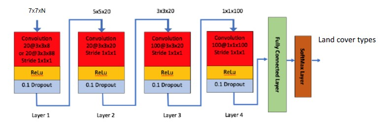
For this CNN-based method, we used the same structure that was used in our previous work [39]. Only the filter size in the first convolution layer was changed accordingly to be consistent with the input patch sizes. This CNN model has four convolutional layers, with various filter sizes and a fully connected layer with 100 hidden units as shown in Figure 1. When we designed the network, we tried different configurations for the number of layers and the size of each layer and selected the one that provided the best results. We did this for all the layers (convolutional and FC layers). The choice of “100 hidden units” was the outcome of our design studies. This model was also used for soil detection due to illegal tunnel excavation, as described in [48]. Each convolutional layer utilizes the Rectified Linear Unit (ReLu) as the activation function. The last fully connected layer uses the SoftMax function for classification. We added dropout layer for each convolutional layer with a dropout rate of 0.1 to mitigate overfitting [49]. It should be noted that the network size changes depending on the input size. In Figure 1, the network should be the same for 5 × 5 as for 7 × 7. The only difference would be that the first layer is deleted. For 3 × 3, the first two layers are deleted. The number of bands (N) in the input image can be any integer number.

2.2. CNN-3D

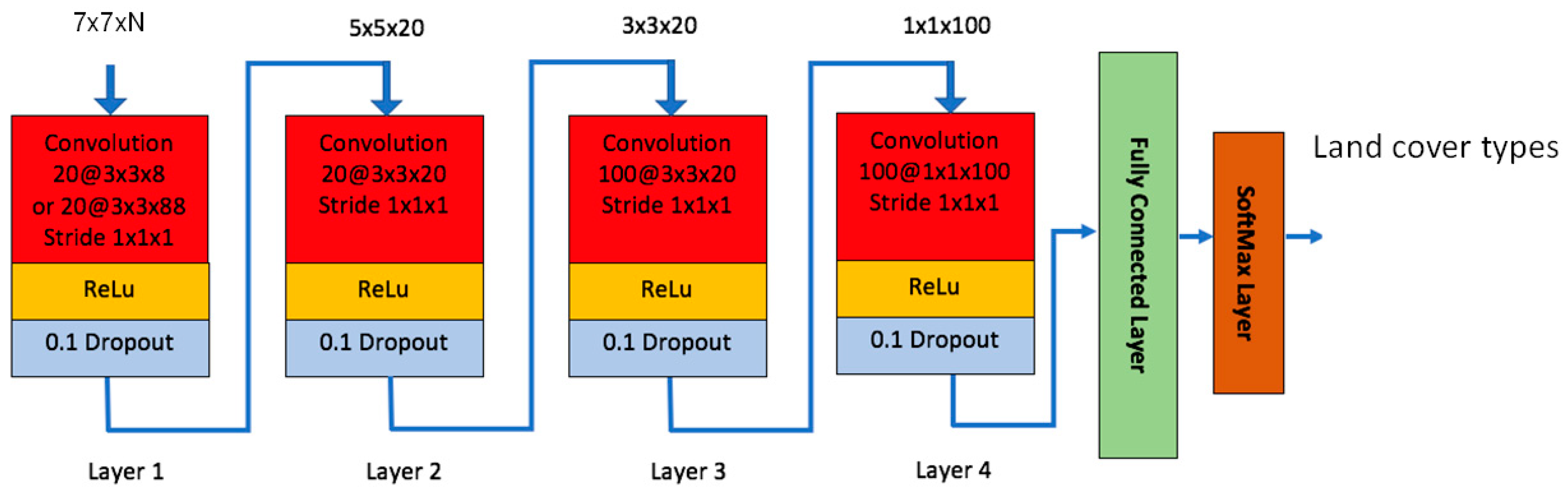
CNN-3D is a CNN-based method [50] with two convolutional layers and two fully connected layers. The two convolutional layers have pooling units and all of its four layers have ReLu units. Figure 2 shows the architecture of this second CNN-based method that is used for land cover classification. This network was used in hyperspectral pixel classification before. The details have been described by the authors of [50]. Due to the use of pooling layers, the patch size cannot be too small. Otherwise, the later layers will not have any impacts.

2.3. EMAP

For a grayscale image $f$ and a sequence of threshold levels $\{T{h}_1, T{h}_2, \dots T{h}_n\}$, the attribute profile (AP) of $f$ was obtained by applying a sequence of thinning and thickening attribute transformations to every pixel in $f$ as follows:

$$AP\left(f\right)=\{{\varphi }_1\left(f\right), {\varphi }_2\left(f\right), \dots {\varphi }_n\left(f\right),f, {\gamma }_1\left(f\right), {\gamma }_2\left(f\right), \dots {\gamma }_n\left(f\right)\}$$

(1)

where ${\varphi }_i$ and ${\gamma }_i \left(i=1, 2, \dots n\right)$ are the thickening and thinning operators at threshold $T{h}_i$, respectively. The EMAP of $f$ was then acquired by stacking two or more APs using any feature reduction technique on multispectral/hyperspectral data, such as purely geometric attributes (e.g., area, length of the perimeter, image moments, shape factors), or textural attributes (e.g., range, standard deviation, entropy) [36,39,40,41] as shown in (2). Further technical details about EMAP can be found in [36,39,40,41].

$$EMAP\left(f\right)=\left\{A{P}_1\left(f\right), A{P}_2\left(f\right) \dots A{P}_m\left(f\right)\right\}$$

(2)

When generating the EMAP-augmented bands in the conducted investigations, no feature dimension reduction process was applied to the hyperspectral data (such as Principal Component Analysis) because the hyperspectral bands of interest were only RGB+NIR instead of all the hyperspectral bands available. EMAP was directly applied to these limited number of bands (RGB+NIR) with the selected attribute profiles, which were the ‘area (a)’ and ‘length of the diagonal of the bounding box’ (d) [43]. The lambda parameters in EMAP for both ‘area’ and ‘length of the diagonal of the bounding box’ attributes were arbitrarily chosen. For the ‘area’ attribute, which is related to modeling spatial information, the higher number of extrema (lambda parameters) contains more detail, whereas the smaller number smooths out the input data. In this work, smoothing was favored and the lambda parameters for the area attribute of EMAP, which is a sequence of thresholds used by the morphological attribute filters, were set to 10 and 15, respectively. For the ‘length of the diagonal of the bounding box’ attribute, which is related to the shape of the regions, the lambda parameters were set to 50, 100, and 500. With these two attributes and their parameter settings, 10 augmented bands were generated for a single band image. The total number of image bands becomes 11 when including the original single band image, Because the resultant EMAP augmented bands were few in number, no feature dimension reduction process was applied to the augmented EMAP bands and all of the EMAP augmented bands were used with the deep learning classifiers.

2.4. Dataset

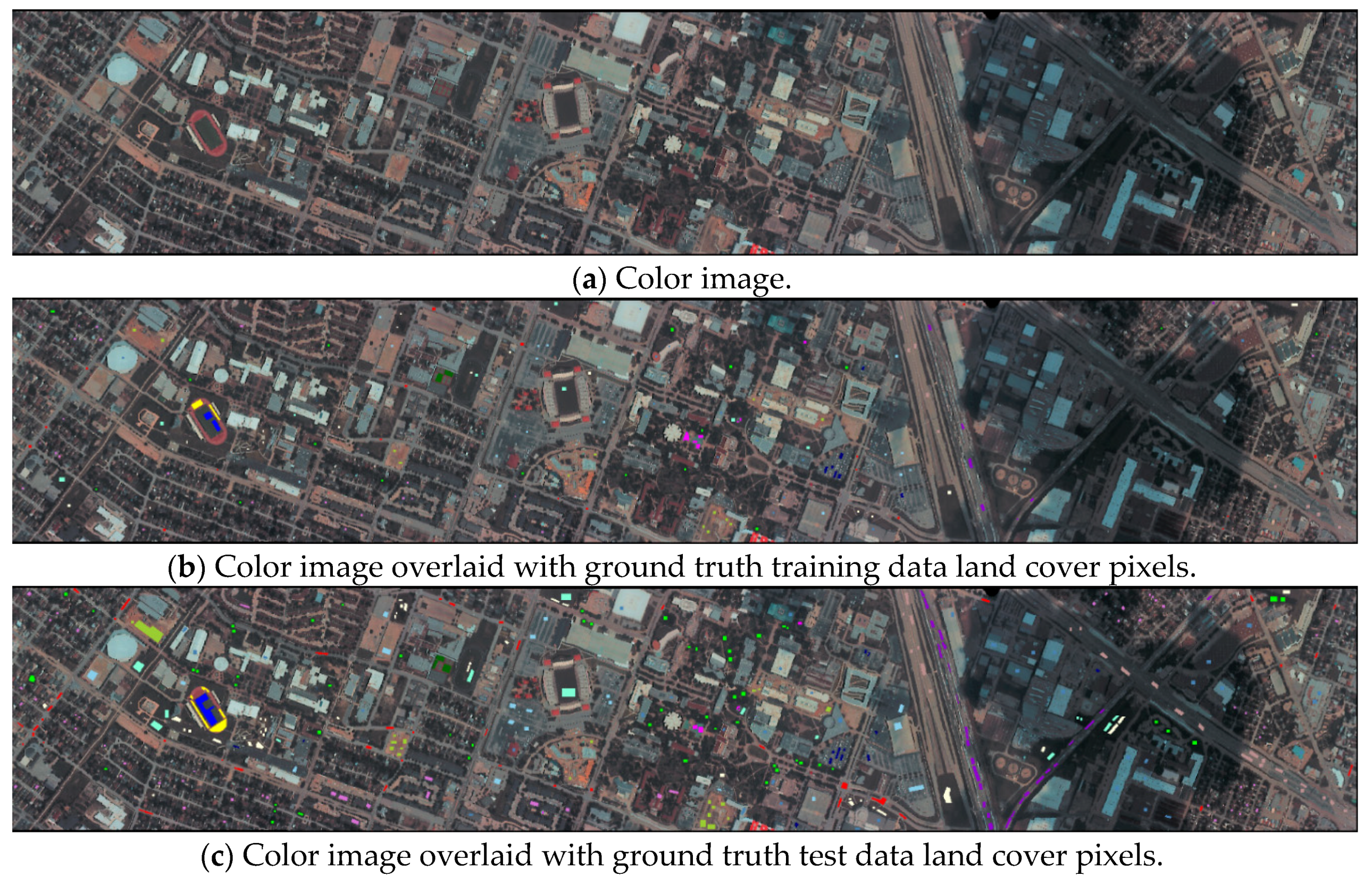
The hyperspectral image dataset for the University of Houston area and the corresponding LiDAR data were used in this paper. This dataset, together with its ground truth land cover maps, were obtained from the IEEE GRSS Data Fusion package [44] and were used in the 2013 IEEE Geoscience and Remote Sensing Society Data Fusion Contest. The hyperspectral data in this dataset contain 144 bands ranging in wavelength values from 380 mm to 1050 nm with a spectral width of 4.65 nm and a spatial resolution of 2.5 m per pixel. The LiDAR data contain the height information and have a resolution of 2.5 m per pixel.

Table 1. Number of pixels per class in the IEEE GRSS data. Total number of unlabeled pixels is 649,816, and total number of pixels is 664,845.

Class
Name	Number	Color Legend	Samples
			Train	Test
Healthy grass	1		198	1053
Stressed grass	2		190	1064
Synthetic grass	3		192	505
Tree	4		188	1056
Soil	5		186	1056
Water	6		182	143
Residential	7		196	1072
Commercial	8		191	1053
Road	9		193	1059
Highway	10		191	1036
Railway	11		181	1054
Parking lot 1	12		192	1041
Parking lot 2	13		184	285
Tennis court	14		181	247
Running track	15		181	473
	1–15		2832	12,197

displays the number of training and test data pixels per land cover class provided in this dataset. There were 15 land cover classes which were identified and named by the contest. These classes and their corresponding training and test datasets (each pixel in the training and test dataset had its own land cover class label) were fixed. The training data set included 2832 pixels and the test dataset includes the remaining 12,197 labeled pixels. Figure 3a shows the color image, and Figure 3b,c show the color image with ground truth land cover annotations for both the training and test dataset. The brightness and contrast of the color image in Figure 3 was adjusted for better visual assessment.

In the hyperspectral image, the investigations with the four bands (RGB+NIR) correspond to the narrow hyperspectral bands, which were directly retrieved from hyperspectral data. These bands are Red (R), Green (G), Blue (Blue), and NIR, and the band numbers in the hyperspectral data for RGB and NIR bands are (R), #30 (G), #22 (B), and #103 (NIR).

We would like to mention that there is another dataset known as Trento data that contains both hyperspectral and LiDAR images. However, the Trento dataset is no longer publicly available to researchers.

2.5. Performance Metrics

For classification performance evaluation of the deep learning methods with EMAP-augmented bands and all other band combinations, we used overall accuracy, OA, which is the ratio of the sum of correctly classified pixels from all classes to the total number of pixels in the test data. In addition to OA, we also generated average accuracy, AA, value which corresponds to the average of individual class accuracies, which is also known as ‘balanced accuracy’. The last performance metric was the well-known Kappa (K) coefficient [51].

3. Results

3.1. Our Customized CNN Results

Table 2. Classification results obtained by our customized CNN model for the considered test dataset with six different sets of image bands. Bold numbers indicate best performing datasets for each row.

Bands	4 Band		4 Band+Lidar		44 Band EMAP		55 Band EMAP		144 Band		144 Band+Lidar
Patch Size	3	5	3	5	3	5	3	5	3	5	3	5
OA (%)	0.7844	0.8108	0.7990	0.7990	0.8792	0.8602	0.8602	0.8429	0.8148	0.8050	0.7878	0.8097
AA (%)	0.8103	0.8364	0.8224	0.8264	0.8982	0.8830	0.8840	0.8670	0.8436	0.8365	0.8202	0.8365
K	0.7661	0.7947	0.7818	0.7825	0.8694	0.8487	0.8492	0.8304	0.8001	0.7898	0.7713	0.7949
(ID)-Class Type (%)
1-Healthy grass	0.8224	0.8234	0.8205	0.8224	0.8310	0.8310	0.8234	0.8310	0.8158	0.8262	0.8167	0.8234
2-Stressed grass	0.8449	0.8449	0.8421	0.8459	0.8393	0.8205	0.8487	0.7162	0.8449	0.8402	0.8355	0.8421
3-Synthetic grass	0.9426	0.9109	0.9485	0.8792	1.0000	1.0000	0.9941	0.9980	0.9861	0.9287	0.9762	0.9822
4-Trees	0.9252	0.9195	0.8958	0.9223	0.9896	0.9271	0.9574	0.9261	0.9157	0.9299	0.9271	0.9138
5-Soil	0.9792	0.9934	0.9735	0.9915	0.9943	1.0000	1.0000	0.9991	0.9848	0.9991	0.9886	0.9943
6-Water	0.8462	0.9301	0.8462	0.9231	0.9510	0.9580	0.9650	0.9021	0.9301	0.9441	0.9441	0.9021
7-Residential	0.8647	0.8918	0.8909	0.8386	0.8647	0.9347	0.8750	0.8675	0.7687	0.8349	0.7724	0.7817
8-Commercial	0.5404	0.6277	0.5850	0.6068	0.7873	0.6021	0.6135	0.5470	0.6638	0.6980	0.5252	0.7227
9-Road	0.6959	0.7866	0.7592	0.7460	0.8659	0.8234	0.8527	0.8036	0.7224	0.7063	0.8083	0.7545
10-Highway	0.5531	0.5010	0.6120	0.5154	0.6844	0.6400	0.6371	0.8070	0.6091	0.4952	0.4373	0.6004
11-Railway	0.6803	0.7021	0.6774	0.6812	0.8634	0.8966	0.8681	0.8662	0.7676	0.7078	0.7277	0.7457
12-Parking lot 1	0.7166	0.8444	0.7301	0.8309	0.9193	0.9462	0.9452	0.8674	0.8357	0.7800	0.7954	0.7032
13-Parking lot 2	0.8035	0.8737	0.8316	0.8596	0.8842	0.8702	0.8877	0.8737	0.8596	0.9088	0.8035	0.8807
14-Tennis Court	0.9798	0.9919	0.9676	0.9838	1.0000	1.0000	1.0000	1.0000	0.9879	0.9595	0.9960	0.9514
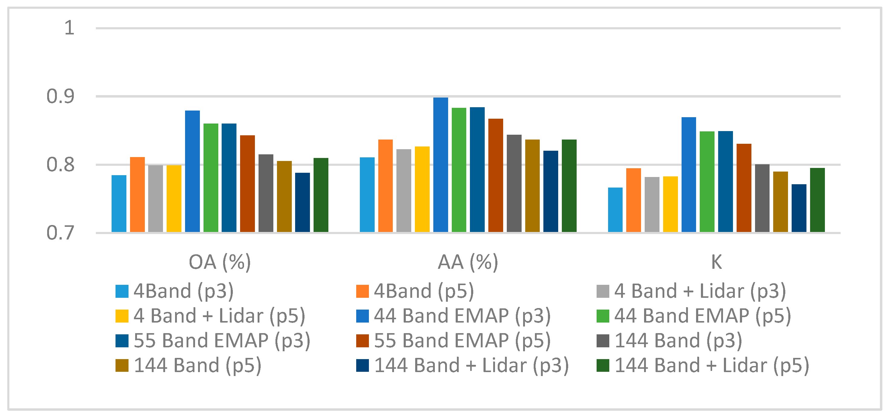
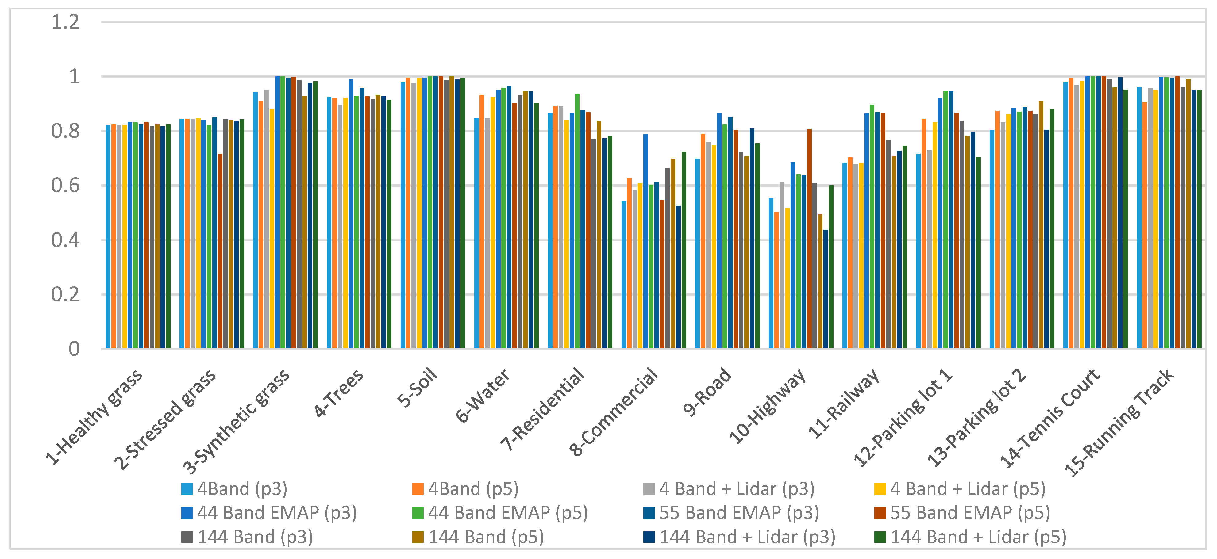
15-Running Track	0.9598	0.9049	0.9556	0.9493	0.9979	0.9958	0.9915	1.0000	0.9619	0.9894	0.9493	0.9493

shows our customized CNN model [48] classification results for the test dataset with six different sets of image bands. These six different sets of image bands are: (a) RGB+NIR (four bands), (b) RGB+NIR+LiDAR (5 bands), (c) 44 EMAP-augmented bands (RGB+NIR bands augmented to 44 bands with EMAP, 11 × 4 = 44), (d) 55 EMAP-augmented bands (RGB+NIR+LiDAR bands augmented to 55 bands with EMAP), (e) 144 hyperspectral bands, and (f) 144 hyperspectral bands+LiDAR (145 bands). The results in Table 2 consist of two parts. The first part corresponds to the resultant performance metrics (OA, AA, and Kappa), and the second part corresponds to the correct classification accuracy for each land cover type using the investigated band combinations with our customized CNN model. Figure 4 and Figure 5 show these results using bar chart type of plots. When applying the customized CNN model, two different patch sizes were investigated, 3 × 3 and 5 × 5, respectively. In Figure 4 and Figure 5, the value in parenthesis after the band combination type corresponds to patch size. As an example, (p3) indicates a patch size of 3 × 3.

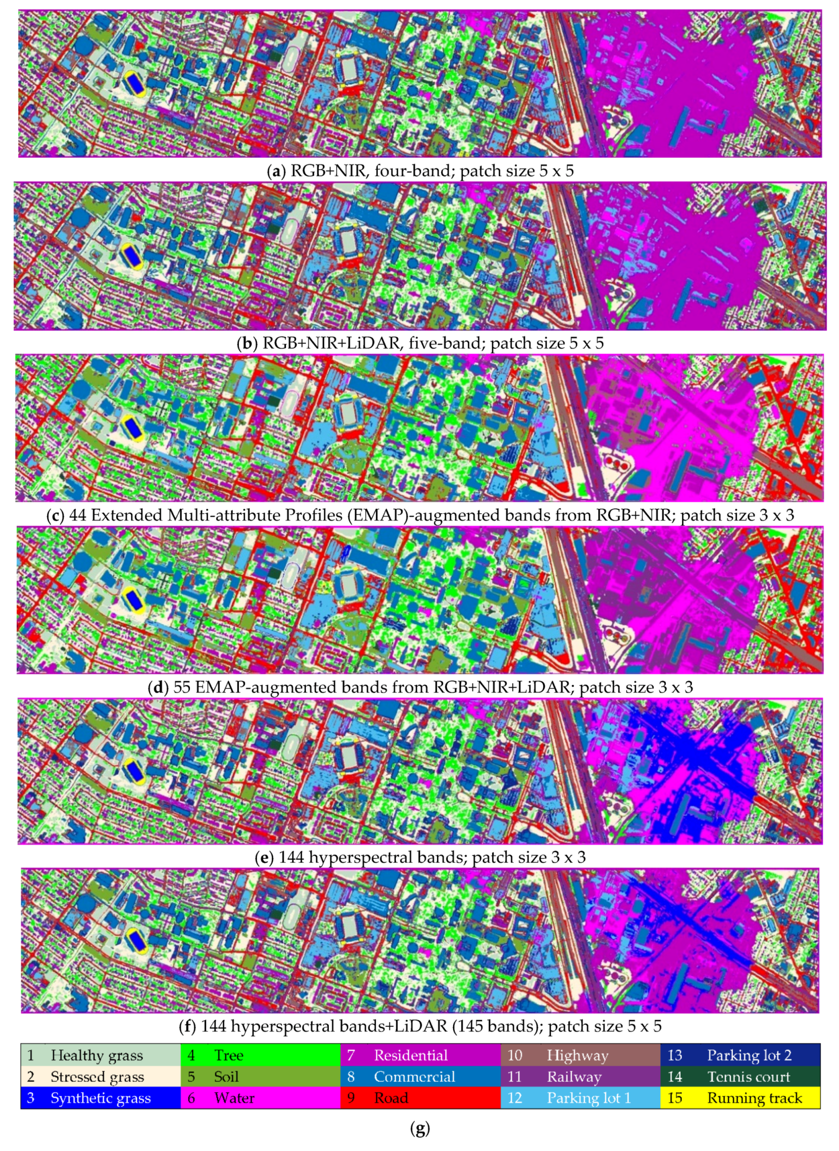
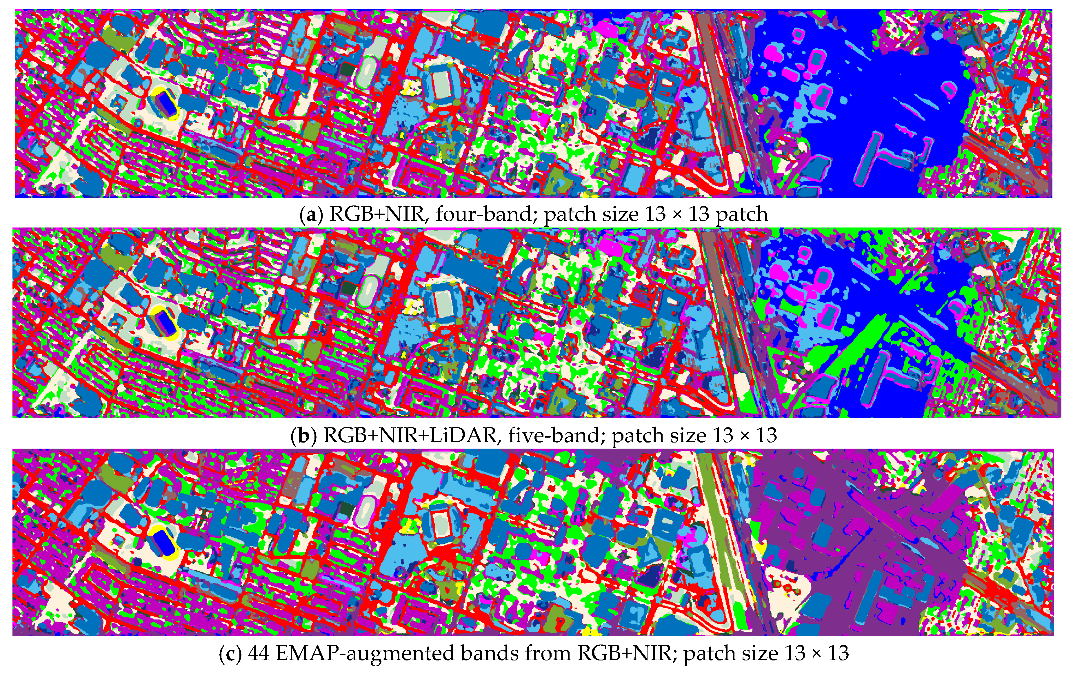
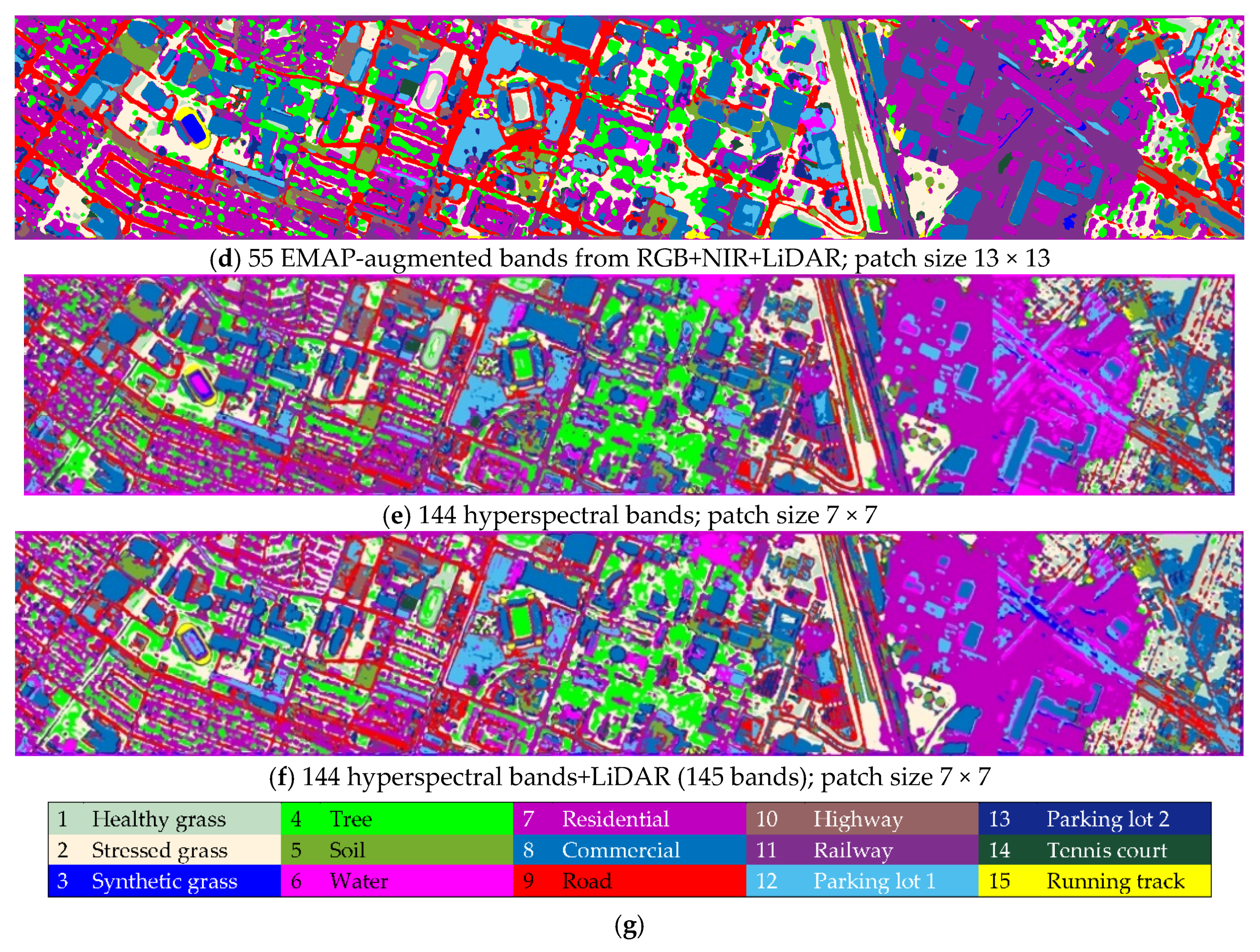
The highest classification accuracy was found to be with the 44 EMAP-augmented bands case using the 3 × 3 patch size, followed by the 55 EMAP-augmented bands case with 3 × 3 patch size. Among the 15 different land covers, two land covers, synthetic grass and tennis court, had perfect correct classification followed by close-to-perfect classification accuracy for soil land cover. The lowest classification accuracy was found to be for highway class. Figure 6 shows the estimated land cover maps for the whole image with our customized CNN model. The estimated land cover map with the highest overall accuracy for each image band set is shown in Figure 6.

3.2. CNN-3D (C3D) Results

Table 3. CNN-3D classification results for the test dataset with six different sets of image bands. Bold numbers indicate best performing datasets for each row.

Bands	4 Band		4 Band+Lidar		44 Band EMAP		55 Band EMAP		144 Band	144 Band +Lidar
Patch Size	13	17	13	17	13	17	13	17	7	7
OA (%)	0.7536	0.6179	0.7843	0.7066	0.8764	0.8634	0.8796	0.8755	0.8010	0.8000
AA (%)	0.7503	0.6767	0.7825	0.6933	0.8816	0.8530	0.8918	0.8756	0.8245	0.8243
K	0.7332	0.6634	0.7663	0.6824	0.8657	0.8515	0.8692	0.8648	0.7850	0.7840
(ID)-Class Type (%)
1-Healthy grass	0.8006	0.8224	0.8291	0.7930	0.8215	0.8405	0.8310	0.8357	0.8433	0.8471
2-Stressed grass	0.8365	0.8026	0.8571	0.8449	0.7641	0.7575	0.7961	0.7735	0.8496	0.8600
3-Synthetic grass	0.5782	0.4396	0.6277	0.4990	0.9901	0.9980	0.9921	0.9683	0.7881	0.7842
4-Trees	0.9375	0.8627	0.9261	0.8930	0.9271	0.9252	0.9129	0.9290	0.8892	0.8902
5-Soil	0.9299	0.9375	0.9574	0.9403	0.9867	0.9877	0.9934	0.9962	0.9858	0.9886
6-Water	0.8252	0.7762	0.9021	0.7552	0.8601	0.7832	0.9441	0.8741	0.9790	0.9441
7-Residential	0.8424	0.8312	0.8526	0.8256	0.9160	0.8937	0.9226	0.8909	0.8657	0.8554
8-Commercial	0.5954	0.5090	0.7056	0.5024	0.7787	0.8053	0.7255	0.7578	0.5812	0.5793
9-Road	0.7573	0.8083	0.8074	0.8215	0.9292	0.9424	0.9207	0.9396	0.7677	0.8017
10-Highway	0.5792	0.3842	0.6274	0.4151	0.6892	0.6641	0.6844	0.7008	0.5956	0.4884
11-Railway	0.6309	0.5066	0.5968	0.5313	0.9839	0.8975	0.9810	0.9592	0.6973	0.7116
12-Parking lot 1	0.7666	0.7003	0.8002	0.7493	0.9222	0.9577	0.9385	0.9712	0.8271	0.8204
13-Parking lot 2	0.8035	0.7579	0.8421	0.7404	0.8596	0.8421	0.8667	0.7860	0.9228	0.9088
14-Tennis Court	0.8664	0.8421	0.8097	0.8502	0.9919	0.7976	0.9798	0.9757	0.9231	0.8907
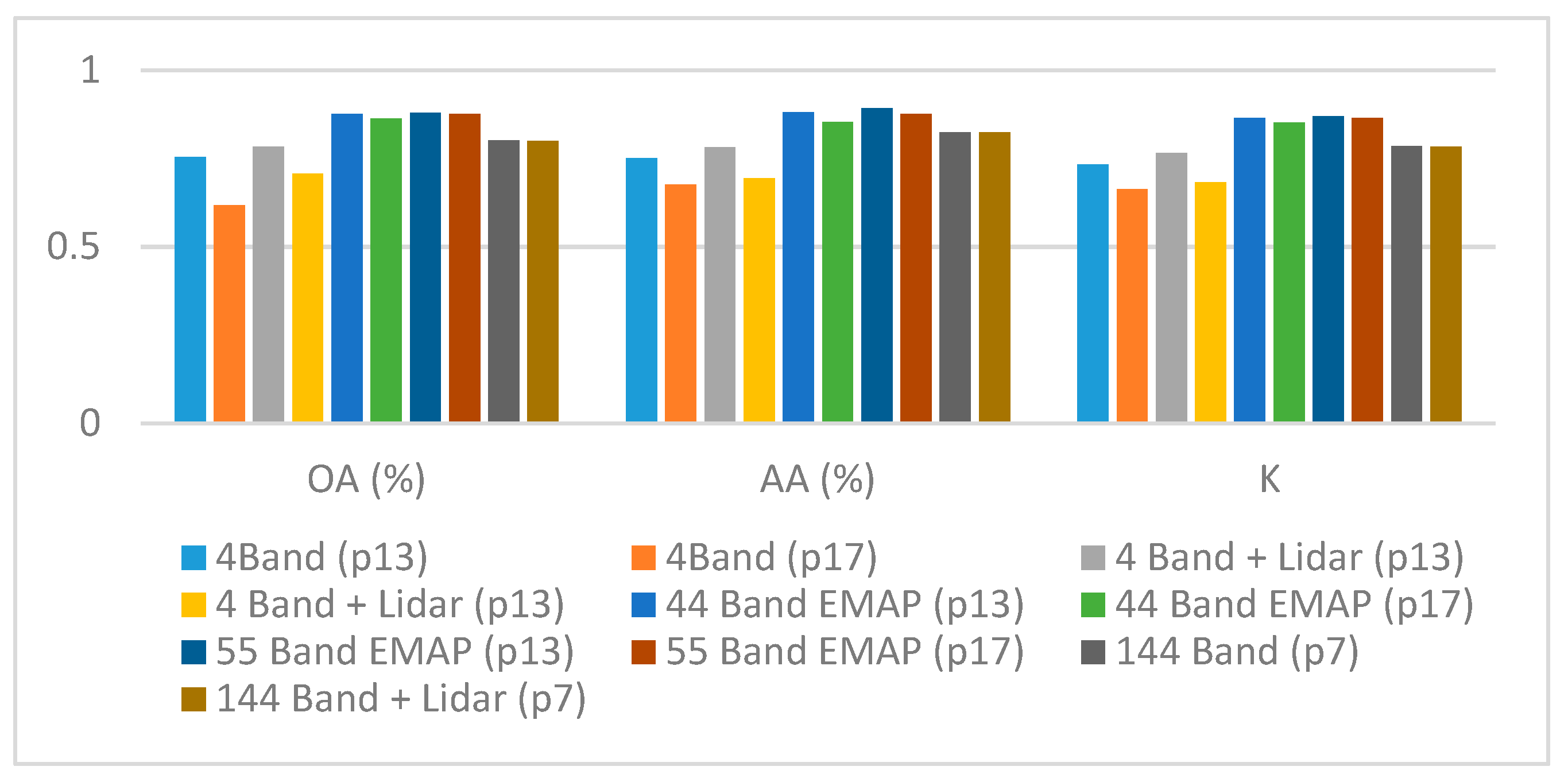
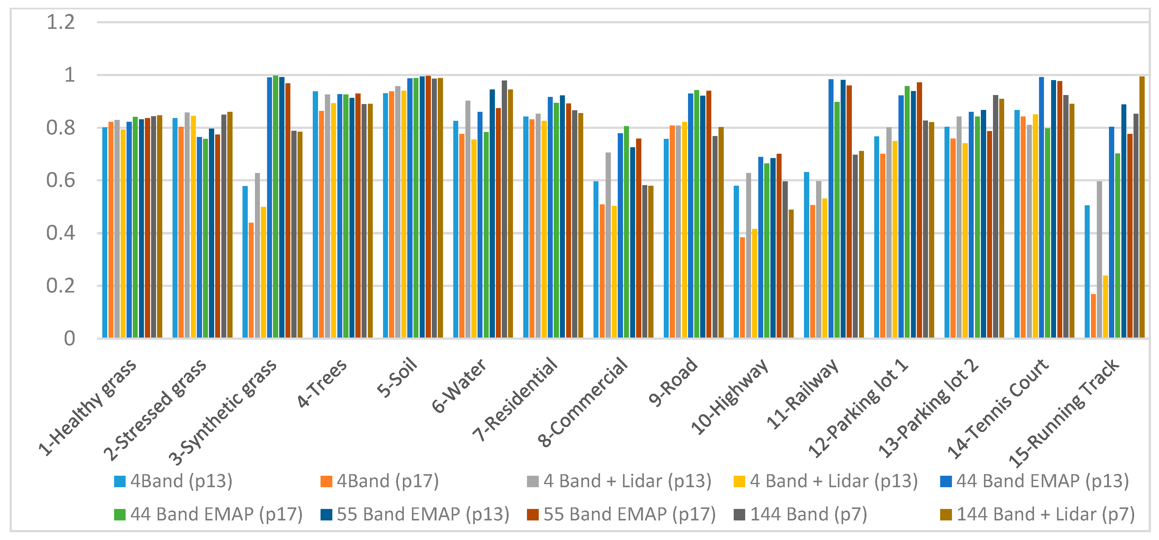
15-Running Track	0.5053	0.1691	0.5962	0.2389	0.8034	0.7019	0.8879	0.7759	0.8520	0.9937

shows the classification results of the CNN-3D method [49] for the test dataset with six different sets of image bands. With this method, two different patch sizes, 13 × 13 and 17 × 17, were investigated for three of the five sets of bands. As mentioned earlier, the patch sizes cannot be too small due to the pooling layers in C3D. For instance, if the patch size is 7 × 7, the patch size will drop to single digits after the first two layers, hence the network cannot function as desired. For the two remaining band sets, which were 144 hyperspectral bands and the 144 hyperspectral bands+LiDAR, the GPU memory was not sufficient for CNN-3D to run. Consequently, only the patch size of 7 × 7 was considered for 144 hyperspectral bands and the 144 hyperspectral bands+LiDAR cases. Even though comparing the 7 × 7 patch size results of these two image band sets with the 13 × 13 and 17 × 17 patch size results of the other three image band sets would not be fair, we still included these results in Table 3 to provide some rough idea about the impact of adding LiDAR band to the hyperspectral bands. Figure 7 corresponds to the bar chart of the resultant performance metrics (OA, AA, and Kappa), and Figure 8 shows the bar chart plot of the correct classification accuracy for each land cover type using the investigated band combinations with CNN-3D model in Table 3.

With CNN-3D, the highest classification accuracy was obtained with the 55 EMAP-augmented bands and 44 EMAP-augmented bands cases using a patch size of 13 × 13. The 55 EMAP-augmented bands case was observed to have slightly higher accuracy than the 44 EMAP-augmented bands case. The classification results with all other image band sets had relatively lower values. For the 55 EMAP-augmented bands case, the top three close-to-perfect correct classifications were for the soil, synthetic grass, and tennis court land covers, whereas the lowest classification accuracy was for highway class. In our customized CNN model results, similar observations were made with respect to the land covers with best top three and the worst classification accuracies. Figure 9 shows the estimated land cover maps with this method for the whole image. For image band sets with more than one investigated patch window size, the one providing better classification performance is shown in Figure 9.

3.3. Performance Comparison of Deep Learning Methods

Table 4. Classification performance comparison of the two deep learning methods for the test dataset with six different image band sets (best performances are highlighted in bold for each image band set).

CNN
Bands	4 Band		4 Band+LiDAR		44 Band EMAP		55 Band EMAP		144 Band		144 Band+ LiDAR
Patch Size	C3D-13	CNN-5	C3D-13	CNN-5	C3D-13	CNN-3	C3D-13	CNN-3	C3D-7	CNN-3	C3D-7	CNN-5
OA (%)	0.7536	0.8108	0.7843	0.7990	0.8764	0.8792	0.8796	0.8602	0.8010	0.8148	0.8000	0.8097
AA (%)	0.7503	0.8364	0.7825	0.8264	0.8816	0.8982	0.8918	0.8840	0.8245	0.8436	0.8243	0.8365
K	0.7332	0.7947	0.7663	0.7825	0.8657	0.8694	0.8692	0.8492	0.7850	0.8001	0.7840	0.7949

shows the highest classification accuracy values obtained with our customized CNN model and CNN-3D method for each of the six image band sets. In five of these six cases, our customized CNN method was observed to perform better than CNN-3D method. The CNN-3D performed better than our customized CNN method only in the 55 EMAP-augmented bands case.

Considering the best classification results from any of the two deep learning methods in each image band set, one interesting observation from Table 5 is that using RGB+NIR bands (four bands) without LiDAR and using hyperspectral bands (144 bands) without the LiDAR resulted in slightly better classification accuracies than the same cases which included LiDAR. For the 44 EMAP-augmented bands case and 55 EMAP-augmented bands case, a similar observation was made when the average accuracy and Kappa metrics were taken into consideration instead of the overall accuracy metric, since these two metrics were found to be slightly higher in the 44 EMAP-augmented bands case in comparison to the 55 EMAP-augmented bands case. For the overall accuracy metric, they were also very close to each other in value. Considering the results with and without LiDAR in these three cases, it was observed that including LiDAR did not seem to have a considerable impact with the deep learning methods. This is somewhat not intuitive, since LiDAR was expected to bring valuable information with respect to height. This could be because several of the 15 land covers in this dataset are surface-level type land covers, meaning they have similar heights with the exception of trees, residential, and commercial land covers. When looking at the classification accuracies of these three land cover classes for the LiDAR-added cases to see whether LiDAR had any impact, mixed results were also seen. It was anticipated that no significant impact of LiDAR would be observed with the two deep learning methods because their classification performances were already good when using RGB+NIR bands.

By comparing the classification maps of Figure 6 and Figure 9, it can be seen that our customized CNN results look crisper due to the use of small patch sizes. In a nutshell, the two CNNs differed only in the pooling layers. In our investigations, we found that the pooling layers did not help the overall classification performance.

3.4. Comparison with Conventional Methods

The deep learning methods’ best classification performances for 44 EMAP-augmented bands and 55 EMAP-augmented bands cases were compared with two conventional methods, Joint Sparse Representation (JSR) [14] and Support Vector Machine (SVM) [47], using the same two sets of EMAP-augmented bands (44 and 55). JSR is more computationally demanding, as it exploits neighborhood pixels for joint land type classification. In JSR, a 3 × 3 or 5 × 5 patch of pixels is used in the S target matrix. The parameter $s_0$ in Equation (13) of [52] is the design parameter, which controls the number of sparse elements. Details of the mathematics have been described by the authors of [52]. We chose that parameter to be 10e-4. There were two SVM parameters, the penalty factor C and the radial basis function (RBF) kernel width, $\gamma$, which were chosen to be 10 and 0.1, respectively. In addition to these two conventional methods, classification results reported by two papers, which used this same dataset with hyperspectral and LiDAR bands augmented with EMAP, were also considered for comparison as well. Details of the JSR and SVM results have been described by the authors of [52].

The resultant overall accuracies of these methods are shown in Table 5. The two conventional methods were observed to perform extremely close in accuracy to the deep learning methods for the 55 EMAP-augmented bands case. For the 44 EMAP-augmented bands case, on the other hand, the deep learning methods’ performances were considerably better than the conventional methods. From Table 5, it can be noticed that adding the LiDAR band to the RGB+NIR bands for EMAP augmentation made a significant impact in overall classification accuracy with the conventional classifiers, JSR and SVM, for land cover classification. However, no considerable impact was observed when adding the LiDAR band to the the EMAP augmentation with the deep learning methods as discussed before.

In [44], the authors investigated three different combinations of hyperspectral bands for land cover classification. Among these, the investigation which used the hyperspectral bands, additional bands from LiDAR data, and the EMAP-augmented hyperspectral bands resulted in an overall accuracy values of 90.65%, whereas the overall accuracy when using only the hyperspectral bands and EMAP-augmented hyperspectral bands was 84.40%. In another paper [53], a graph-based approach was proposed to fuse HS and LiDAR data for land cover classification. In [53], the authors used the same dataset with three different band combinations. Their investigation with hyperspectral bands only using SVM classifier had an accuracy of 80.72%. Our results using only hyperspectral bands are in line with this result, since we reached an accuracy of 81.48% using our customized CNN method, which provided slightly higher accuracy than their result. A second investigation described by the authors of [53] used the morphological profiles of hyperspectral and LiDAR bands and reached an accuracy of 86.39%.

In our case, even though only four bands (RGB+NIR) and five bands (RGB+NIR+LiDAR) were used with EMAP for augmentation, decent classification accuracies of 87.92% (Our CNN) and 87.96% (CNN-3D) were reached, respectively. These overall accuracy values are higher than the investigations described by the authors of [44,53], which used all hyperspectral bands and additional LiDAR bands together with EMAP augmentation. This is quite impressive considering that we augmented only four bands with EMAP instead of using all hyperspectral bands and additional bands from LiDAR and still reached an overall accuracy of 87.92%. Our work shows that with deep learning methods using a fewer number of bands and utilizing EMAP augmentation, it is possible to arrive at very decent correct classification accuracies for land cover classification, eliminating the need of using hundreds of hyperspectral bands. This could ultimately reduce computation and data storage needs.

Table 5. Comparison of the overall accuracies (%) of several methods.

Reference	Dataset Adopted	Algorithm Adopted	Overall Accuracy
[52]	44 EMAP (RGB+NIR)	JSR	80.77
[52]	44 EMAP (RGB+NIR)	SVM	82.64
This paper	44 EMAP (RGB+NIR)	Our CNN	87.92
This paper	44 EMAP (RGB+NIR)	CNN-3D	87.64
[52]	55 EMAP (RGB+NIR+LiDAR)	JSR	86.86
[52]	55 EMAP (RGB+NIR+LiDAR)	SVM	86.00
This paper	55 EMAP (RGB+NIR+LiDAR)	Our CNN	86.02
This paper	55 EMAP (RGB+NIR+LiDAR)	CNN-3D	87.96
[44]	Hyperspectral data; EMAP augmentation applied hyperspectral data (Xh + EMAP(Xh))	MLRsub	84.40
	Hyperspectral data; Additional bands from LiDAR data (Xh + AP(XL))	MLRsub	87.91
	Hyperspectral data; EMAP augmentation applied hyperspectral data; Additional bands from LiDAR data (Xh + AP(XL) + EMAP(Xh))	MLRsub	90.65
[53]	Hyperspectral data	SVM	80.72
	Morphological Profile of hyperspectral and LiDAR data (MPSHSLi)	SVM	86.39

Table 5. Comparison of the overall accuracies (%) of several methods.

Reference	Dataset Adopted	Algorithm Adopted	Overall Accuracy
[52]	44 EMAP (RGB+NIR)	JSR	80.77
[52]	44 EMAP (RGB+NIR)	SVM	82.64
This paper	44 EMAP (RGB+NIR)	Our CNN	87.92
This paper	44 EMAP (RGB+NIR)	CNN-3D	87.64
[52]	55 EMAP (RGB+NIR+LiDAR)	JSR	86.86
[52]	55 EMAP (RGB+NIR+LiDAR)	SVM	86.00
This paper	55 EMAP (RGB+NIR+LiDAR)	Our CNN	86.02
This paper	55 EMAP (RGB+NIR+LiDAR)	CNN-3D	87.96
[44]	Hyperspectral data; EMAP augmentation applied hyperspectral data (Xh + EMAP(Xh))	MLRsub	84.40
	Hyperspectral data; Additional bands from LiDAR data (Xh + AP(XL))	MLRsub	87.91
	Hyperspectral data; EMAP augmentation applied hyperspectral data; Additional bands from LiDAR data (Xh + AP(XL) + EMAP(Xh))	MLRsub	90.65
[53]	Hyperspectral data	SVM	80.72
	Morphological Profile of hyperspectral and LiDAR data (MPSHSLi)	SVM	86.39

Here, we compared the computational costs of different methods. We used a desktop PC with i7 quadcore CPU and a GPU (NVIDIA GeForce Titan X Pascal 12GB GDDR5X). The JSR and SVM results only used CPU, and the CNN and C3D used GPU.

Table 6. Computational times in minutes for different methods and datasets. CNN and C3D used GPU, whereas JSR and SVM used CPU only.

Computational Times (min)	4 Band	4 Band+LiDAR	44 Band EMAP	55 Band EMAP	144 Band	144 Band+LiDAR
CNN	<1	<1	~1.5	~1.5	~3	~3
C3D	<1	<1	~1	~1.5	~3	~3
JSR	629.23	891.71	2248.17	2198.56	2210.15	2310.42
SVM	5.32	3.76	0.69	0.47	1.30	1.41

summarizes the computational times in minutes. It can be seen that SVM were much faster than JSR because JSR needed a lot more time in minimizing the sparseness constraint. The CNN and C3D times are similar and less than three minutes, which might be misleading. It should be noted that the deep learning methods all used GPU, hence the computational times are less than those conventional methods.

4. Conclusions

In this paper, we investigated the classification performance of two deep learning methods for land cover classification, where only four bands (RGB+NIR) and five bands (RGB+NIR+LiDAR) were used in terms of EMAP augmentation. In the performance evaluations, the RGB+NIR bands and hyperspectral bands were used without EMAP as well. The results showed that, using deep learning methods and EMAP augmentation, RGB+NIR (four bands) or RGB+NIR+LiDAR (five bands) can produce very good classification performance, and these results are better than those obtained by conventional classifiers such as SVM and JSR. We observed that, even though adding LiDAR band to RGB+NIR bands for augmentation made a significant classification performance impact with respect to conventional classifiers (JSR and SVM), no significant impact was observed with the deep learning methods, since their classification performances were already very good when using RGB+NIR bands. This work demonstrated that using RGB+NIR (four bands) or RGB+NIR+LiDAR (five bands) with EMAP augmentation is feasible for land cover classification, as the resultant accuracies are only a few percentage points lower than some of the best performing methods in the literature which used the same dataset and utilized all the available hyperspectral bands.

The fusion of different classifiers using decision level fusion [54] or pixel level fusion [55] could be a good future direction. Parallel implementation of JSR and SVM using parallel processing techniques could be another future direction.

References

- Ayhan, B.; Kwan, C.; Jensen, J.O. Remote vapor detection and classification using hyperspectral images. In Proceedings of the SPIE 11010, Chemical, Biological, Radiological, Nuclear, and Explosives (CBRNE) Sensing XX, Baltimore, MD, USA, 14 May 2019; p. 110100U. [Google Scholar]
- Kwan, C.; Ayhan, B.; Chen, G.; Chang, C.; Wang, J.; Ji, B. A Novel Approach for Spectral Unmixing, Classification, and Concentration Estimation of Chemical and Biological Agents. IEEE Trans. Geosci. Remote Sens. 2006, 44, 409–419. [Google Scholar] [CrossRef]
- Harsanyi, J.C.; Chang, C.I. Hyperspectral image classification and dimensionality reduction: An orthogonal subspace projection approach. IEEE Trans. Geosci. Remote Sens. 1994, 32, 779–785. [Google Scholar] [CrossRef] [Green Version]
- Heinz, D.C.; Chang, C.I. Fully constrained least squares linear spectral mixture analysis method for material quantification in hyperspectral imagery. IEEE Geosci. Remote Sens. Soc. 2001, 39, 529–545. [Google Scholar] [CrossRef] [Green Version]
- Dao, M.; Kwan, C.; Ayhan, B.; Tran, T. Burn Scar Detection Using Cloudy MODIS Images via Low-rank and Sparsity-based Models. In Proceedings of the IEEE Global Conference on Signal and Information Processing (GlobalSIP), Washington, DC, USA, 7–9 December 2016; pp. 177–181. [Google Scholar]
- Veraverbeke, S.; Dennison, P.; Gitas, I.; Hulley, G.; Kalashnikova, O.; Katagis, T.; Kuai, L.; Meng, R.; Roberts, D.; Stavros, N. Hyperspectral remote sensing of fire: State-of-the-art and future perspectives. Remote Sens. Environ. 2018, 216, 105–121. [Google Scholar] [CrossRef]
- Wang, W.; Li, S.; Qi, H.; Ayhan, B.; Kwan, C.; Vance, S. Identify Anomaly Component by Sparsity and Low Rank. In Proceedings of the 7th Workshop on Hyperspectral Image and Signal Processing: Evolution in Remote Sensing (WHISPERS), Tokyo, Japan, 2–5 June 2015. [Google Scholar]
- Chang, C.-I. Hyperspectral Imaging; Springer: New York, NY, USA, 2003. [Google Scholar]
- Li, S.; Wang, W.; Qi, H.; Ayhan, B.; Kwan, C.; Vance, S. Low-rank Tensor Decomposition based Anomaly Detection for Hyperspectral Imagery. In Proceedings of the IEEE International Conference on Image Processing (ICIP), Quebec City, QC, Canada, 27–30 September 2015; pp. 4525–4529. [Google Scholar]
- Yang, Y.; Zhang, J.; Song, S.; Liu, D. Hyperspectral Anomaly Detection via Dictionary Construction-Based Low-Rank Representation and Adaptive Weighting. Remote Sens. 2019, 11, 192. [Google Scholar] [CrossRef] [Green Version]
- Qu, Y.; Guo, R.; Wang, W.; Qi, H.; Ayhan, B.; Kwan, C.; Vance, S. Anomaly Detection in Hyperspectral Images through Spectral Unmixing and Low Rank Decomposition. In Proceedings of the IEEE International Geoscience and Remote Sensing Symposium (IGARSS), Beijing, China, 10–15 July 2016; pp. 1855–1858. [Google Scholar]
- Li, F.; Zhang, L.; Zhang, X.; Chen, Y.; Jiang, D.; Zhao, G.; Zhang, Y. Structured Background Modeling for Hyperspectral Anomaly Detection. Sensors 2018, 18, 3137. [Google Scholar] [CrossRef] [Green Version]
- Qu, Y.; Qi, H.; Ayhan, B.; Kwan, C.; Kidd, R. Does Multispectral/Hyperspectral Pansharpening Improve the Performance of Anomaly Detection? In Proceedings of the IEEE International Geoscience and Remote Sensing Symposium (IGARSS), Fort Worth, TX, USA, 23–28 July 2017; pp. 6130–6133. [Google Scholar]
- Dao, M.; Kwan, C.; Koperski, K.; Marchisio, G. A Joint Sparsity Approach to Tunnel Activity Monitoring Using High Resolution Satellite Images. In Proceedings of the IEEE Ubiquitous Computing, Electronics & Mobile Communication Conference, New York, NY, USA, 19–21 October 2017; pp. 322–328. [Google Scholar]
- Radke, R.J.; Andra, S.; Al-Kofani, O.; Roysam, B. Image change detection algorithms: A systematic survey. IEEE Trans. Image Proc. 2005, 14, 294–307. [Google Scholar] [CrossRef]
- İlsever, M.; Unsalan, C. Two-Dimensional Change Detection Methods; Springer: Berlin, Germany, 2012. [Google Scholar]
- Zhou, J.; Kwan, C.; Ayhan, B.; Eismann, M. A Novel Cluster Kernel RX Algorithm for Anomaly and Change Detection Using Hyperspectral Images. IEEE Trans. Geosci. Remote Sens. 2016, 54, 6497–6504. [Google Scholar] [CrossRef]
- Bovolo, F.; Bruzzone, L. The time variable in data fusion: A change detection perspective. IEEE Geosci. Remote Sens. Mag. 2015, 3, 8–26. [Google Scholar] [CrossRef]
- Kwan, C.; Haberle, C.; Echavarren, A.; Ayhan, B.; Chou, B.; Budavari, B.; Dickenshied, S. Mars Surface Mineral Abundance Estimation Using THEMIS and TES Images. In Proceedings of the IEEE Ubiquitous Computing, Electronics & Mobile Communication Conference, New York, NY, USA, 8–10 November 2018. [Google Scholar]
- CRISM. Available online: http://crism.jhuapl.edu/ (accessed on 18 December 2019).
- Lindgren, D. Land Use Planning and Remote Sensing; Taylor & Francis: Milton Park, UK, 1984; Volume 2. [Google Scholar]
- Gu, Y.; Jin, X.; Xiang, R.; Wang, Q.; Wang, C.; Yang, S. UAV-Based Integrated Multispectral-LiDAR Imaging System and Data Processing. Sci. China Technol. Sci. 2020, 1–9. [Google Scholar] [CrossRef]
- Jahan, F.; Zhou, J.; Awrangjeb, M.; Gao, Y. Inverse Coefficient of Variation Feature and Multilevel Fusion Technique for Hyperspectral and LiDAR Data Classification. IEEE J. Sel. Top. Appl. Earth Obs. Remote Sens. 2020, 13, 367–381. [Google Scholar] [CrossRef] [Green Version]
- Wu, Y.; Zhang, X. Object-Based Tree Species Classification Using Airborne Hyperspectral Images and LiDAR Data. Forests 2020, 11, 32. [Google Scholar] [CrossRef] [Green Version]
- Hänsch, R.; Hellwich, O. Fusion of Multispectral LiDAR, Hyperspectral, and RGB Data for Urban Land Cover Classification. IEEE Geosci. Remote Sens. Lett. 2020. [Google Scholar] [CrossRef]
- Tusa, E.; Laybros, A.; Monnet, J.M.; Dalla Mura, M.; Barré, J.B.; Vincent, G.; Dalponte, M.; Feret, J.-P.; Chanussot, J. Fusion of hyperspectral imaging and LiDAR for forest monitoring. In Data Handling in Science and Technology; Elsevier: Amsterdam, The Netherlands, 2020; Volume 32, pp. 281–303. [Google Scholar]
- Du, Q.; Ball, J.E.; Ge, C. Hyperspectral and LiDAR data fusion using collaborative representation. Algorithms Technol. Appl. Multispectr. Hyperspectr. Imagery XXVI 2020, 11392, 1139208. [Google Scholar] [CrossRef]
- Zhang, M.; Li, W.; Du, Q.; Gao, L.; Zhang, B. Feature extraction for classification of hyperspectral and LiDAR data using patch-to-patch CNN. IEEE Trans. Cybern. 2018, 50, 100–111. [Google Scholar] [CrossRef]
- Mei, X.; Pan, E.; Ma, Y.; Dai, X.; Huang, J.; Fan, F.; Du, Q.; Zheng, H.; Ma, J. Spectral-spatial attention networks for hyperspectral image classification. Remote Sens. 2019, 11, 963. [Google Scholar] [CrossRef] [Green Version]
- Senecal, J.J.; Sheppard, J.W.; Shaw, J.A. Efficient Convolutional Neural Networks for Multi-Spectral Image Classification. In Proceedings of the International Joint Conference on Neural Networks (IJCNN), Budapest, Hungary, 14–19 July 2019; pp. 1–8. [Google Scholar]
- Zhang, X.; Han, L.; Han, L.; Zhu, L. How Well Do Deep Learning-Based Methods for Land Cover Classification and Object Detection Perform on High Resolution Remote Sensing Imagery? Remote Sens. 2020, 12, 417. [Google Scholar] [CrossRef] [Green Version]
- Audebert, N.; Saux, B.L.; Lefevre, S. Semantic Segmentation of Earth Observation Data Using Multimodal and Multi-scale Deep Networks. arXiv 2016, arXiv:1609.06846. [Google Scholar]
- Huang, B.; Zhao, B.; Song, Y. Urban land-use mapping using a deep convolutional neural network with high spatial resolution multispectral remote sensing imagery. Remote Sens. Environ. 2018, 214, 73–86. [Google Scholar] [CrossRef]
- Kemker, R.; Salvaggio, C.; Kanan, C. Algorithms for Semantic Segmentation of Multispectral Remote Sensing Imagery using Deep Learning. ISPRS J. Photogramm. Remote Sens. 2018, 145, 60–77. [Google Scholar] [CrossRef] [Green Version]
- Zheng, C.; Wang, L. Semantic Segmentation of Remote Sensing Imagery Using Object-Based Markov Random Field Model with Regional Penalties. IEEE J. Sel. Top. Appl. Earth Obs. Remote Sens. 2015, 8, 1924–1935. [Google Scholar] [CrossRef]
- Mura, M.D.; Benediktsson, J.A.; Waske, B.; Bruzzone, L. Extended profiles with morphological attribute filters for the analysis of hyperspectral data. Int. J. Remote Sens. 2010, 31, 5975–5991. [Google Scholar] [CrossRef]
- Shu, W.; Liu, P.; He, G.; Wang, G. Hyperspectral Image Classification Using Spectral-Spatial Features with Informative Samples. IEEE Access 2019, 7, 20869–20878. [Google Scholar] [CrossRef]
- Zaatour, R.; Bouzidi, S.; Zagrouba, E. Impact of Feature Extraction and Feature Selection Techniques on Extended Attribute Profile-based Hyperspectral Image Classification. In Proceedings of the 12th International Joint Conference on Computer Vision, Imaging and Computer Graphics Theory and Applications (VISIGRAPP 2017), Porto, Portugal, 27 February–1 March 2017; pp. 579–586. [Google Scholar]
- Bernabe, S.; Marpu, P.R.; Plaza, A.; Benediktsson, J.A. Spectral unmixing of multispectral satellite images with dimensionality expansion using morphological profiles. In Proceedings of the SPIE Satellite Data Compression, Communications, and Processing VIII, San Diego, CA, USA, 19 October 2012; Volume 8514, p. 85140Z. [Google Scholar]
- Mura, M.D.; Benediktsson, J.A.; Waske, B.; Bruzzone, L. Morphological attribute profiles for the analysis of very high resolution images. IEEE Trans. Geosci. Remote Sens. 2010, 48, 3747–3762. [Google Scholar] [CrossRef]
- Bernabe, S.; Marpu, P.R.; Plaza, A.; Mura, M.D.; Benediktsson, J.A. Spectral–spatial classification of multispectral images using kernel feature space representation. IEEE Geosci. Remote Sens. Lett. 2014, 11, 288–292. [Google Scholar] [CrossRef]
- Ghamisi, P.; Benediktsson, J.A.; Cavallaro, G.; Plaza, A. Automatic framework for spectral–spatial classification based on supervised feature extraction and morphological attribute profiles. IEEE J. Sel. Top. Appl. Earth Obs. Remote Sens. 2014, 7, 2147–2160. [Google Scholar] [CrossRef]
- Dao, M.; Kwan, C.; Bernabe, S.; Plaza, A.; Koperski, K. A Joint Sparsity Approach to Soil Detection Using Expanded Bands of WV-2 Images. IEEE Geosci. Remote Sens. Lett. 2019, 1–5. [Google Scholar] [CrossRef]
- Khodadadzadeh, M.; Li, J.; Prasad, S.; Plaza, A. Fusion of Hyperspectral and LiDAR Remote Sensing Data Using Multiple Feature Learning. IEEE J. Sel. Top. Appl. Earth Obs. Remote Sens. 2015, 8, 2971–2983. [Google Scholar] [CrossRef]
- Li, S.; Qiu, J.; Yang, X.; Liu, H.; Wan, D.; Zhu, Y. A novel approach to hyperspectral band selection based on spectral shape similarity analysis and fast branch and bound search. Eng. Appl. Artif. Intell. 2014, 27, 241–250. [Google Scholar] [CrossRef] [Green Version]
- Feng, F.; Li, W.; Du, Q.; Zhang, B. Dimensionality reduction of hyperspectral image with graph-based discriminant analysis considering spectral similarity. Remote Sens. 2017, 9, 323. [Google Scholar] [CrossRef] [Green Version]
- Burges, C. A Tutorial on Support Vector Machines for Pattern Recognition. Data Mining and Knowledge Discovery; Kluwer Academic Publishers: Boston, MA, USA, 1998; pp. 121–167. [Google Scholar]
- Perez, D.; Banerjee, C.; Kwan, M.; Dao, Y.; Shen, K.; Koperski, G.; Marchisio, G.; Li, J. Deep Learning for Effective Detection of Excavated Soil Related to Illegal Tunnel Activities. In Proceedings of the IEEE Ubiquitous Computing Electronics and Mobile Communication Conference, New York, NY, USA, 19–21 October 2017; pp. 626–632. [Google Scholar]
- Srivastava, N.; Hinton, G.; Krizhevsky, A.; Sutskever, I.; Salakhutdinov, R. Dropout: A simple way to prevent neural networks from overfitting. J. Mach. Learn. Res. 2014, 15, 1929–1958. [Google Scholar]
- Deep Learning for HSI Classification. Available online: https://github.com/luozm/Deep-Learning-for-HSI-classification (accessed on 21 April 2020).
- Cardillo, G. Cohen’s Kappa: Compute the Cohen’s Kappa Ratio on a 2 × 2 Matrix. Available online: https://www.github.com/dnafinder/Cohen (accessed on 22 April 2020).
- Kwan, C.; Gribben, D.; Ayhan, B.; Bernabe, S.; Plaza, A.; Selva, M. Improving Land Cover Classification Using Extended Multi-attribute Profiles (EMAP) Enhanced Color, Near Infrared, and LiDAR Data. Remote Sens. 2020, 26, 1392. [Google Scholar] [CrossRef]
- Liao, W.; Pižurica, A.; Bellens, R.; Gautama, S.; Philips, W. Generalized Graph-Based Fusion of Hyperspectral and LiDAR Data Using Morphological Features. IEEE Geosci. Remote Sens. Lett. 2015, 12, 552–556. [Google Scholar] [CrossRef]
- Safont, G.; Salazar, A.; Vergara, L. Multiclass alpha integration of scores from multiple classifiers. Neural Comput. 2019, 31, 806–825. [Google Scholar] [CrossRef] [PubMed]
- Kwan, C.; Chou, B.; Kwan, L.Y.M.; Larkin, J.; Ayhan, B.; Bell, J.F.; Kerner, H. Demosaicing enhancement using pixel-level fusion. SIViP 2018, 12, 749–756. [Google Scholar] [CrossRef]
Figure 1.
Our customized conventional neural network (CNN) model.
Figure 2.
CNN-3D [50].
Figure 3.
Color image for the University of Houston area with ground truth land cover annotations of test data.
Figure 4.
Performance metrics for the investigated band combinations with our customized CNN model.
Figure 5.
Classification accuracy for each land cover type with our customized CNN model using the investigated band combinations.
Figure 6.
Estimated land cover maps by our customized CNN method for the whole image.
Figure 7.
Performance metrics for the investigated band combinations with the CNN-3D model.
Figure 8.
Classification accuracy for each land cover type with CNN-3D model using the investigated band combinations.
Figure 9.
CNN-3D method estimated land cover maps for the whole image.