Generating Elevation Surface from a Single RGB Remotely Sensed Image Using Deep Learning
by
Emmanouil Panagiotou
1,*,†, 
Georgios Chochlakis
1,†,
Lazaros Grammatikopoulos
2 and
Eleni Charou
3 1
School of Electrical and Computer Engineering, National Technical University of Athens, 15780 Zografou, Greece
2
Department of Surveying and Geoinformatics Engineering, University of West Attica, 12243 Egaleo, Greece
3
Institute of Informatics and Telecommunications, National Centre for Scientific Research Demokritos, 15310 Aghia Paraskevi, Greece
*
Author to whom correspondence should be addressed.
†
These authors contributed equally to this work.
Remote Sens. 2020, 12(12), 2002; https://0-doi-org.brum.beds.ac.uk/10.3390/rs12122002
Submission received: 25 May 2020
/
Revised: 12 June 2020
/
Accepted: 18 June 2020
/
Published: 22 June 2020
(This article belongs to the Special Issue Feature Paper Special Issue: Large Spatial Scale Analysis and Intensive Data Use in Urban Social, Ecological, Economic, or Environmental System)
Abstract
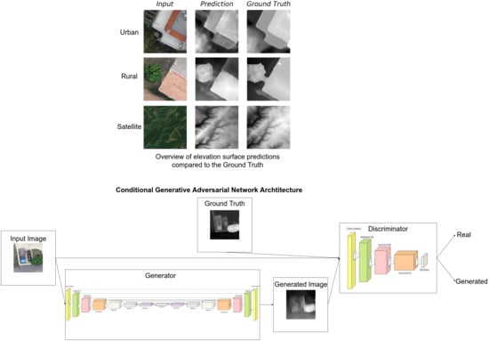
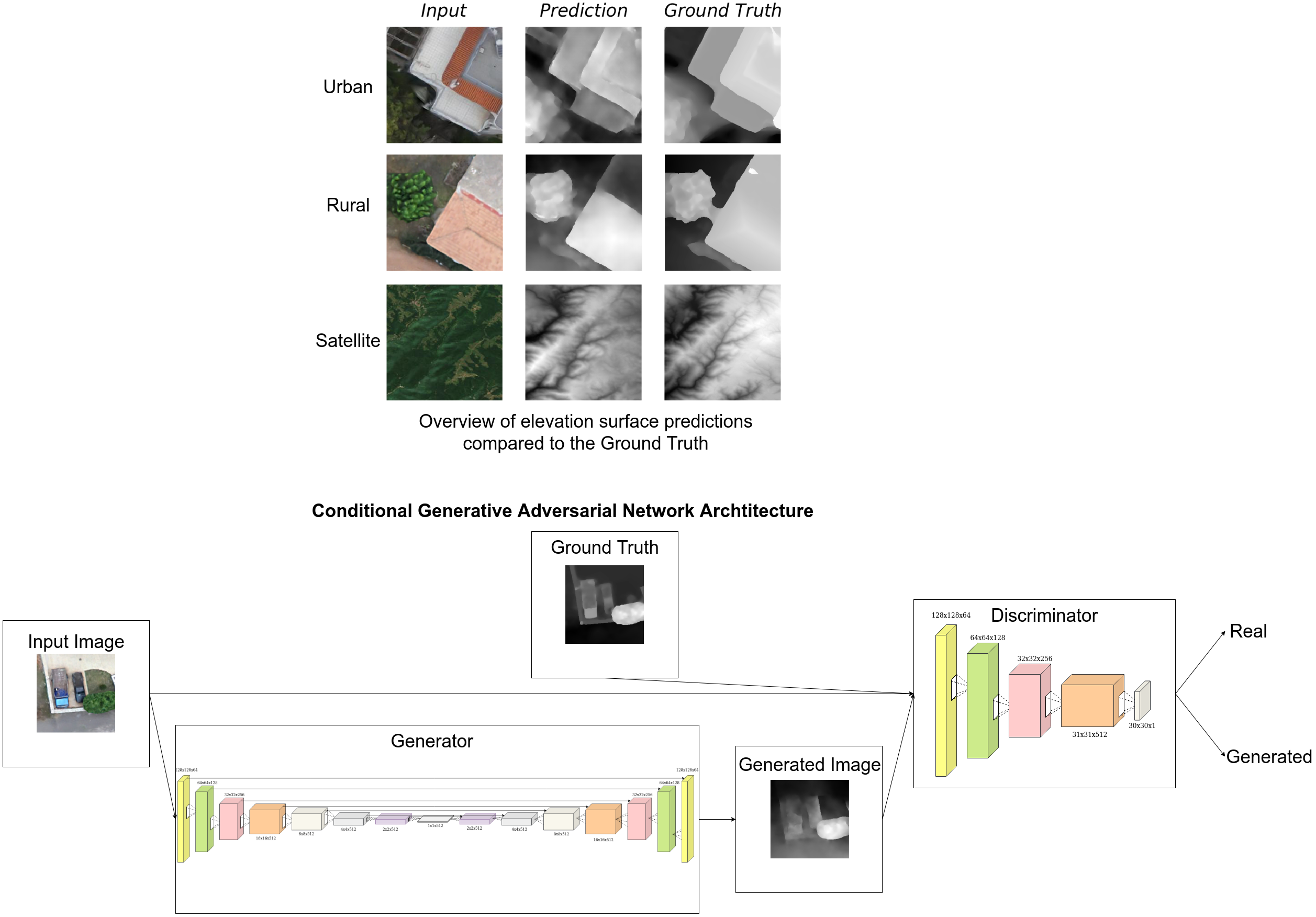
:Generating Digital Elevation Models (DEM) from satellite imagery or other data sources constitutes an essential tool for a plethora of applications and disciplines, ranging from 3D flight planning and simulation, autonomous driving and satellite navigation, such as GPS, to modeling water flow, precision farming and forestry. The task of extracting this 3D geometry from a given surface hitherto requires a combination of appropriately collected corresponding samples and/or specialized equipment, as inferring the elevation from single image data is out of reach for contemporary approaches. On the other hand, Artificial Intelligence (AI) and Machine Learning (ML) algorithms have experienced unprecedented growth in recent years as they can extrapolate rules in a data-driven manner and retrieve convoluted, nonlinear one-to-one mappings, such as an approximate mapping from satellite imagery to DEMs. Therefore, we propose an end-to-end Deep Learning (DL) approach to construct this mapping and to generate an absolute or relative point cloud estimation of a DEM given a single RGB satellite (Sentinel-2 imagery in this work) or drone image. The model has been readily extended to incorporate available information from the non-visible electromagnetic spectrum. Unlike existing methods, we only exploit one image for the production of the elevation data, rendering our approach less restrictive and constrained, but suboptimal compared to them at the same time. Moreover, recent advances in software and hardware allow us to make the inference and the generation extremely fast, even on moderate hardware. We deploy Conditional Generative Adversarial networks (CGAN), which are the state-of-the-art approach to image-to-image translation. We expect our work to serve as a springboard for further development in this field and to foster the integration of such methods in the process of generating, updating and analyzing DEMs.
1. Introduction
A Digital Elevation Model (DEM) is a 3D computer graphics representation of a terrain’s surface. The accessibility to precise DEMs is fundamental for multiple applications such as hydrology and geomorphology [1,2,3,4], water flow [5], 3D flight planning and collision avoidance [6,7], Geographic Information systems (GIS) [8], satellite navigation [9,10], auto-safety, autonomous driving and intelligent transportation systems [11,12,13], precision farming and forestry [14,15], and, of course, 3D visualizations and rectification of aerial photography. This variety of applications and disciplines establishes DEMs as an essential tool that ought to be readily available to researchers and experts. Unfortunately, standard methods for DEM generation, such as airborne Light detection and ranging (Lidar) or Interferometric Synthetic-Aperture Radar (inSAR), remain a bottleneck for such applications and analyses, due to time constraints and high operational cost. Recently, Unmanned Aerial Vehicles (UAVs) have been used to generate DEMs based on an automatic photogrammetric methodology, but although they excel in efficiency and ease, they impose several technical restrictions concerning the image capturing process. These constraints include the need for sophisticated equipment, the precise planning of the capturing mission, the specialized and laborious calibration operation [16], while, simultaneously, many factors have to be taken into consideration regarding the planning and the processing pipeline, such as image overlap, flight altitude, camera and lens characteristics among others [17,18,19].
At its core, the problem of generating DEMs can be formulated as a function G whose input is a representation of the terrain patch of interest (e.g., RGB satellite images) and its output is the DEM itself
where X is the domain of remotely sensed imagery and Y that of DEMs. All other forms of data incorporated in the DEM generation, such as multiple views, could be considered superfluous to the task, albeit mandatory for contemporary techniques. Under this interpretation of the process, an optimal generator would only rely on a single representation of the terrain to produce the correct DEM, assuming that this function is a bijection. While that assumption does not hold, since adding a small constant to the height map may not alter the remotely sensed image, it is an approximation that we assume holds locally, meaning we assume that the ground elevation of a tile has insignificant variation, and auxiliary data within the image, like shadows, can be harnessed to resolve the ambiguities. All that said, obtaining this mapping requires an involved rule-based approach that is impossible to “hard-code”, as the possible configurations of the terrain are effectively endless. On the other hand, Artificial Intelligence (AI) and Machine Learning (ML) can learn such rules in an automated, data-driven manner by building an internal model of the area of interest and its structure. In particular, Deep Learning (DL), the data-intensive version of ML, has recently been proven to be useful for many difficult and ill-posed tasks, such as natural language processing [20,21], computer vision [22,23,24], reinforcement learning [25,26], and many others. Multiple DL algorithms have surpassed human capabilities in areas like visual recognition [27], board games like chess and Go [28], etc. Given this groundbreaking advances, many remote sensing applications have increasingly started deploying DL [29] to improve on prior performance by eliminating “hard-coded” human heuristics from the process. Some general guidelines and approaches are presented in [30,31,32]. Some applications with widespread use involve remote sensing image segmentation and classification [33,34,35], and super-resolution for remote sensing data [36,37]. Few works have applied DL to DEMs, mostly for classification or correction [38,39,40]. Similar work is also carried out in depth estimation [41,42,43,44], where monocular images or video frames are used, and variants of the U-net [45] are deployed, possibly enhanced with residual blocks [46]. Recurrent Neural Networks (RNN) are also used to accommodate the processing of video frames where necessary.
We propose a DL approach for retrieving the aforementioned (approximate) one-to-one mapping, in the form of a point cloud, i.e., every point on the 2D grid of the remotely sensed image is assigned a third coordinate, its height, using Conditional Generative Adversarial Networks (CGAN) and, overall, the possibility of such techniques being an optimal solution for this problem, not necessarily confined within the realm of using just a single datum to produce the DEM. Our approach achieves production of sharp, robust results, whereas its quantitative performance is suboptimal. To compensate for this shortcoming, we thoroughly examine data augmentation techniques (Section 2.8), regularization techniques and perform ablation studies (Section 3.2) which indicate that quantitative performance depends on the amount of data, which we limit due to resource constraints.
2. Materials and Methods
In this section, we provide the necessary background for the utilized methods and describe our techniques and datasets. Readers uncomfortable with any introductory concepts presented below are referred to the excellent introductory, intermediate and advanced material in [47]. Note, however, that contemporary DL frameworks automatically handle many of these technical details and familiarity with them may not be necessary.
2.1. Typical Convolutional Architecture
A Convolutional Neural Network (CNN) is a (deep) neural network, consisting of an input, multiple hidden and an output layer. Every hidden layer is comprised of convolutional layers performing intermediate computations (hence the name hidden). They convolve the input by applying a dot product with a kernel consisting of trainable weights. The output is typically passed by a pooling layer that reduces the input dimensions for the next layer by aggregating local pixel-level information. Compared to standard feedforward neural networks, CNNs are able to make strong hypothesis regarding the nature and structure of the images by zeroing out connections between neurons that are further apart with respect to their position in the image with the use of small kernels and, thus, limiting the receptive fields of neurons, resulting in much fewer connections and parameters and in turn to computationally affordable training times [23].
2.2. Generative Adversarial Networks
Generative Adversarial Networks (GAN) [48] constitute a general framework for training generative models, i.e., models that can produce samples, not only differentiate between them. GANs consist of a generator G and a discriminator D, both modeled as artificial neural networks. The generator is optimized to reproduce the true data distribution , which can be fixed to the distribution of interest, by generating images (or any form of data) that are difficult for the discriminator to differentiate from the real images, namely the actual data distribution . Simultaneously, the discriminator is tasked with differentiating real images from synthetic data generated by G. Their training procedure is a minimax two-player game with the following objective function:
where z is a noise vector sampled from a prior noise distribution of choice , usually a uniform or a normal distribution, and x is a real image, from the data distribution . [48] prove that, given enough capacity, the generator can learn to replicate the true data distribution.
2.3. Conditional Generative Adversarial Networks
As suggested in [48] and first examined in [49], CGANs can extend GANs by incorporating additional information, like a class label or, analogous to our case, extracted features, in effect conditioning the generator and the discriminator to it. Denoting the additional conditioning variable as c, we can substitute and from Equation (1) with and , whereas the rest of the formulation remains the same:
2.4. Architecture Analysis
Deep CNNs have been heavily tested and therefore proven to work on image classification and generative tasks [50,51,52,54], thus we use CNNs for the generator and the discriminator networks.
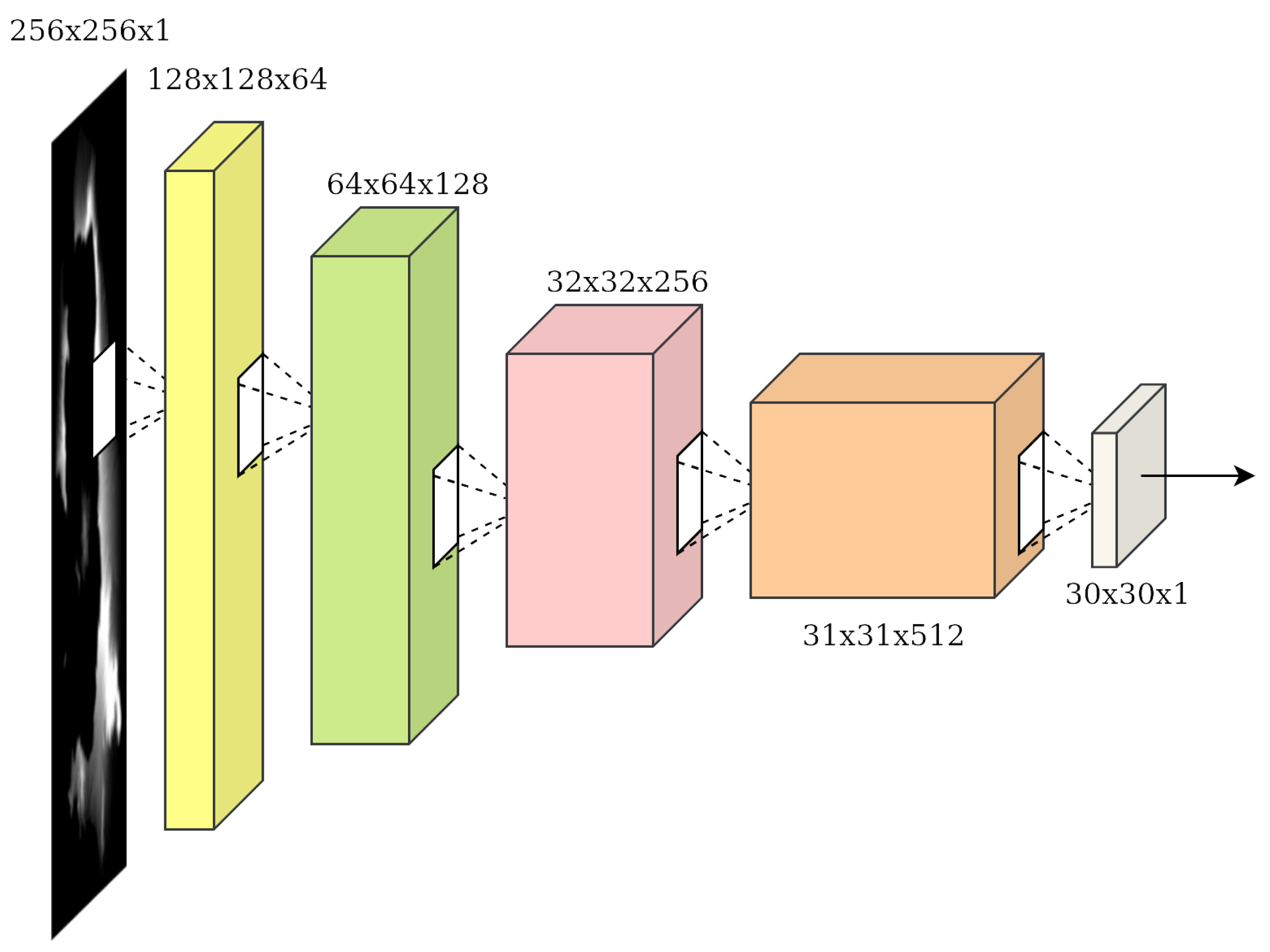
The discriminator’s objective is to utilize convolutional layers to reduce the dimensions of the input images, ending up with a binary output classifying the input images as real or fake (synthesised by the generator). In our case, a PatchGAN is used [55]. The main difference is that the traditional CNN architecture would come to a decision based on the whole input image, whereas the PatchGAN maps the image, in our case, to a square array of outputs. Each output “pixel” signifies whether the corresponding patch is real or fake. The final decision is derived by averaging over all the individual patches. The PatchGAN architecture can be seen in Figure 1.
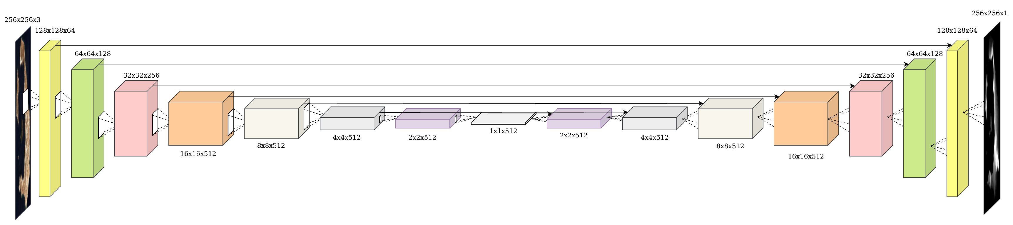
The generator, on the other hand, is a U-net [45], an encoder-decoder architecture. That is to say, the encoder downsamples the conditioning input (e.g., satellite) image down to a bottleneck layer (also denoted as code, hence the name encoder) using a series of convolutional layers. Afterwards, the decoder, through a series of deconvolutions, roughly the inverse operator of the convolution, the images are upsampled, decoding the bottleneck code to the size of the output image. Every convolutional layer in the encoder is connected with a skip connection to its respective deconvolutional layer in the decoder, by concatenating the encoder’s output to the decoder’s input channel-wise, helping the model to converge during training since it skips some layers by feeding the output of one layer as the input to next layers [56]. This facilitates training, provided the low-level structure, which can be thought of as the pixel-level structure, is the same between input and output, as is the case in our area of interest. Certain generators in GAN models, specifically the decoder, receive random noise as additional input, resulting in one-to-many relationships [57]. In our case, such a practice is not only unnecessary but actually detrimental, as we would like to construct a deterministic function, relying solely on the input condition to generate output images. The architecture of the U-net can be seen in Figure 2.
Ultimately, the CGAN we use is pix2pix [55], which combines the U-net and the PatchGAN for training in the CGAN framework. We again note that no noise is used in the architecture, as we model bijections, not one-to-many mappings. The dimensions of the intermediate representations during the training of the full-scale model (as opposed to diminished architecture used in other studies within the paper due to resource constraints) can be seen in Figure 1 and Figure 2. It is also worth mentioning that we use strided convolutions instead of pooling layers to perform the dimensionality reduction in the encoder. These translate to convolutional kernels with a stride, both for the encoder and the decoder. The composition of each block is complemented optionally by batch normalization [58], and a Leaky ReLU for the encoder or a plain ReLU for the decoder [59]. The Leaky ReLU’s coefficient is set to 0.2. We utilize the same convolutional blocks for PatchGAN, except for the last layer where the stride is set to the default .
To evaluate our results and to be consistent with the formulation utilized in [55], we deploy the mean absolute distance (mean L1 error) between each pixel of the generated DEM, , and the ground truth one, y,
Note that compared to other similar norms, the absolute distance weighs fine-grained details and discrepancies equally to larger incongruities, while [55] report that the squared distance yields blurry results. Additionally, to measure realism and punish collapses into coarse approximations, we visually inspect and present our results.
Incorporating the L1 metric into the CGAN framework, the final cost function we are trying to optimize is
which roughly translates, as far as it concerns the generator, to trying to fool the discriminator while also generating accurate DEMs with respect to the ground truth. controls their relative importance.
Note that regularization of the main model is solely achieved with the application of dropout (see Section 2.5 for details) in the first layers of the decoder of the generator, which are responsible for extracting and handling more abstract and high-level concepts and features. To further analyse the efficacy of the model, we conduct more experiments with lightweight and regularized models. To make several runs possible and get more robust results, we reduce the number of samples in the dataset and the size of the model even further.
In more detail, we apply L2 regularization, we punish, that is, the model for “wandering” to regions of the its parameter space where its parameters receive “big” values by adding to the original cost function (Equation (4)) the sum of the squared Frobenius norms of its weight matrices, multiplied by the hyperparameter , namely
where are the trainable parameters of the generator G. In practice, to get a decent understanding of how L2 regularization affects the model’s performance, it is advised to vary the exponent of the hyperparameter and, as an effect, its order of magnitude. Following this practice, we examine our approach’s performance by setting .
Furthermore, we try reducing the number of parameters in the model by reducing the number of layers, decreasing the number of parameters in certain layers or both. Reducing the number of parameters in the model abates its flexibility to adapt to training data, usually resulting in higher bias. However, given that some “smaller” model can confidently fit the training data, reducing the flexibility of the model can yield better validation results, restricting it from adopting ad-hoc behaviors to perfectly fit the training data, hurting generalization. We remove some of the bottleneck layers, symmetrically of course from both the encoder and the decoder of the generator, and/or reduce the filters/channels of each layer significantly.
2.5. Training
During training, our hyperparameters’ configuration follows the ones suggested by [55], i.e., is set to 100, we utilize the ADAM [60] optimizer with a learning rate of 0.0002 and equal to 0.5. We use batch normalization [58] wherever suggested to speed up the training process, along with skipping the bias term, dropout [61] to reduce overfitting. Our implementation uses Tensorflow [62], which is responsible for many of the hyperparameters by virtue of its default values. For more details, the code for our work has been made publicly available at https://github.com/Panagiotou/ImageToDEM.
2.6. Datasets
2.6.1. Satellite Imagery
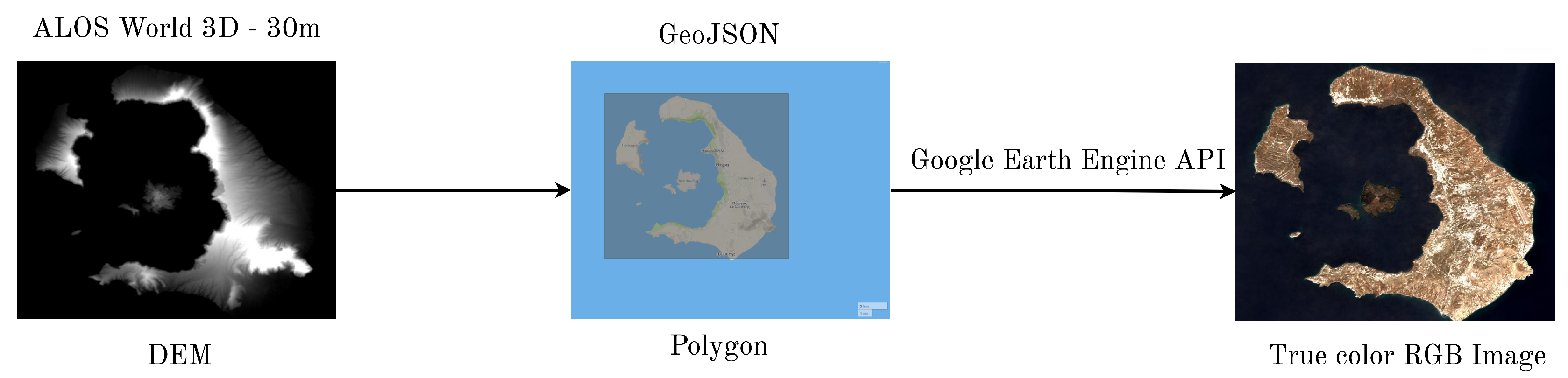
In order for a CNN architecture to be trained, a large-scale dataset is imperative, as well as computing power to process it, preferably with the parallel processing capabilities of a Graphics Processing Unit (GPU). Our task consists of performing an image-to-image translation from RGB satellite images to their corresponding DEMs. During this process the DEM is interpreted as a single band (grayscale) image. Evidently, a dataset of pairs of RGB satellite images and their corresponding DEM images is needed. As we were unable to acquire data containing both RGB and DEM images, we decide to build our own. To be more precise, a large area over Greece was selected as our region of interest (ROI). The DEM images corresponding to our ROI are provided by ALOS Global Digital Surface Model “ALOS World 3D-30 m (AW3D30)” [63] and can be granted with a request to the respective owners. We then split the DEMs into smaller tiles and, for each tile, a script obtains the corresponding RGB tile. In particular, the program extracts a GeoJSON polygon from the georeferenced DEM tile and feeds it to the Google Earth Engine API [64], which is publicly available. This, then, returns the true color bands [TCI_R, TCI_G, TCI_B] Sentinel-2 MSI, which, when stacked, yield the requested RGB satellite image corresponding to the input DEM. To get the final dataset we reshape our data so that all tiles are pixels. The code for the data acquisition is available in the aforementioned repository and can be easily modified to return whichever bands required. The overall process is graphically presented in Figure 3. Some pairs of the dataset can be seen at Figure 4. As a preprocessing step, we project the DEMs to the range, as each tile was scaled to the range according to the global minimum-maximum of the entire dataset.
2.6.2. Multispectral Extension of Satellite Imagery
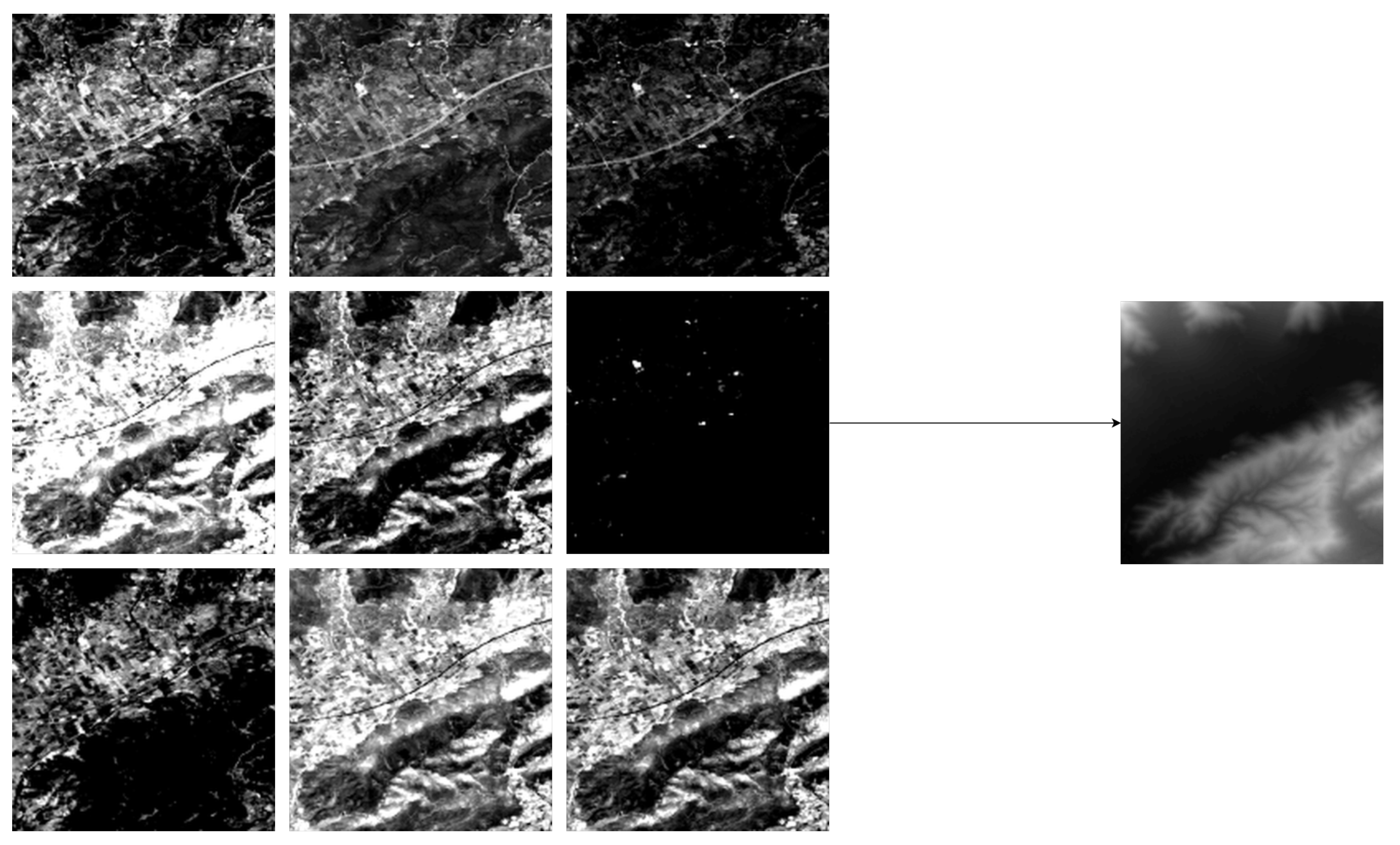
Although the scope of our work is to predict a DEM conditioned to an RGB image, it is meaningful to try to predict the DEM using a Sentinel-2 Multispectral input image. Due to the nature of the model we use, it is very straightforward to add more input channels as long as they retain the same dimensionality i.e., pixels. We utilize a modified version of our script to download and build a dataset of input Multispectral images containing the bands [B2, B3, B4, B5, B6, B7, B8, B8A, B11]. A succinct description of the bands as stated in the Earth Engine Data Catalog can be found at Table 1. A grayscale representation of the bands for a single satellite image along with the corresponding DEM are presented in Figure 5.
2.7. Urban and Rural Drone Imagery
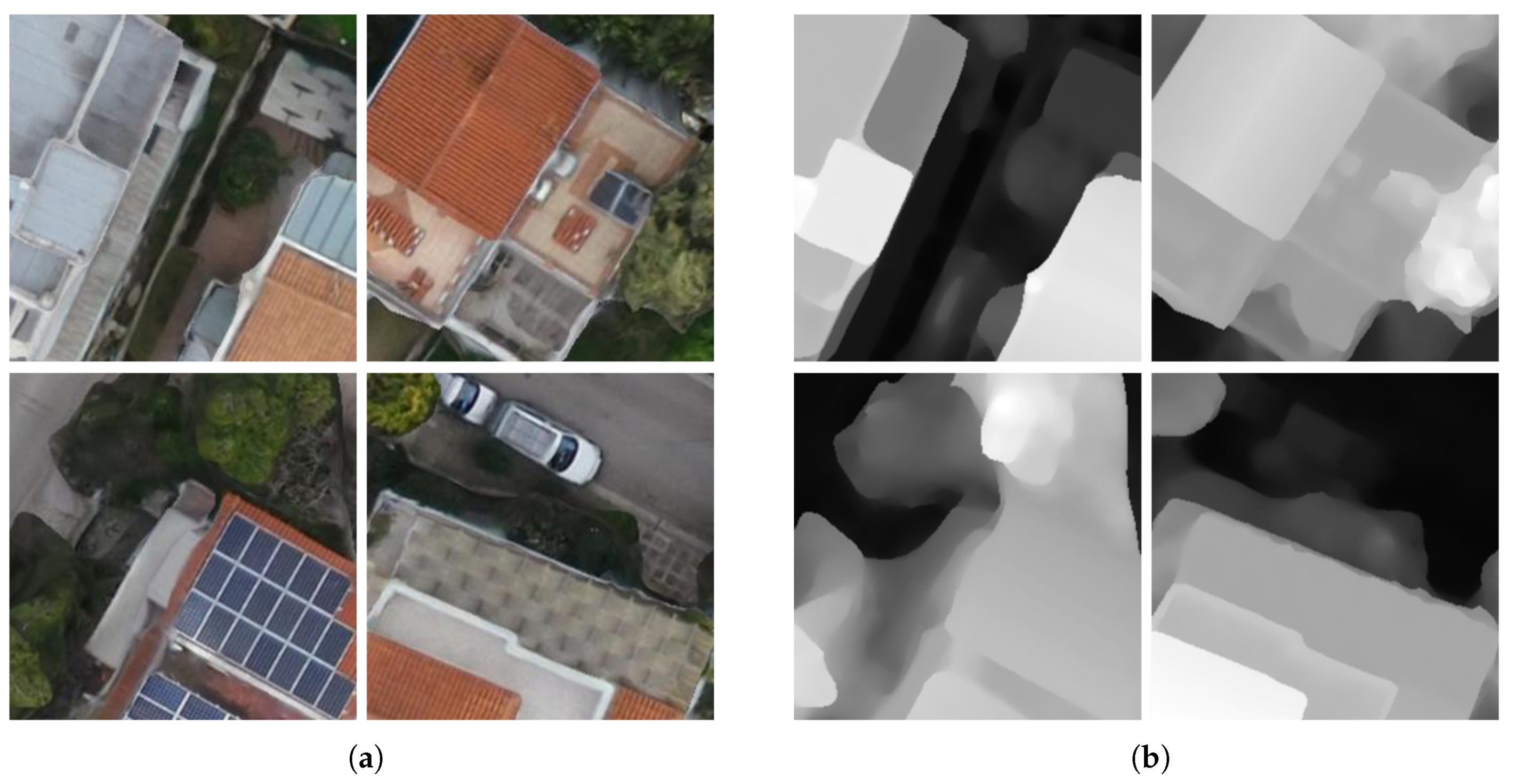
We also utilize the architecture to predict DEM data of urban and rural regions with higher resolution. To demonstrate our approach’s efficacy on this domain, we train on a dataset of drone images in an urban setting and on one in a rural setting. The datasets consist of RGB 8-bit orthophoto images with 5 cm spatial resolution as inputs and a Digital Surface Model (DSM), a height map of both natural and artificial structures, of the same resolution. Note that DEMs subsume DSMs. The datasets have been generated by Map Ltd. (Athens, Greece) [65], specifically for our work, employing a standard photogrammetric approach, based on vertical overlapping RGB images acquired by the drone “eBee plus” (senseFly, Lausanne, Switzerland). Each DSM tile is normalized to the range, based on the local minimum-maximum values of that tile. Higher resolution elevation models that can be captured via Drone or Lidar have much more detail than the DEMs provided by satellites. Therefore, the model has to learn the 3D geometry of more complex structures such as cars, houses, and trees. Samples of the urban and rural drone images are displayed in Figure 6 and Figure 7 respectively.
2.8. Data Augmentation
A useful regularization technique is data augmentation, i.e., augmenting the dataset with samples not originally present in it per se, but derived from the dataset altogether. This especially holds for the satellite-imagery dataset, where overfitting was detected. Namely, the model was unable to generalize its knowledge on previously unseen data in some cases (Section 2.9). The method we follow is: initially, we construct pairs of input-output images of size . Second, we partition those, into more than 4 overlapping tiles, thereby constructing an augmented dataset. In particular, by splitting 2500 satellite images of size into 26 smaller tiles each, we end up with a dataset with approximately 65,000 pairs. Obviously, such an inflation in data implies longer training times but also results in better generalization. Rotations and random crops are also frequently used, but we decided against that, as data interpolation techniques are necessary in these cases, putting the accuracy of the dataset in peril.
2.9. GAN Training and Evaluation Pitfalls
After a GAN is trained, it is essential to evaluate its performance to conclude whether it actually replicates the true data distribution correctly, namely the DEMs in our case. Our main approach is to ensure that the generator loss tends to zero, as it should, given enough training data and computing power. In supervised machine learning, evaluating a model solely on training data provides a heavily biased estimate of the generalization performance, rendering it unable to convey much meaningful information about generalization and overfitting. If and when overfitting occurs, the model is inadequate to generalize its predictions on unseen data. In general, machine learning models that tackle overfitting have low variance (gap between train and test performance) and low bias (train error), meaning that the model has learned rules that are strict enough to depict the learned aspects during training and generic enough to make good predictions on unseen test data. A countermeasure of paramount significance to prevent overfitting is using a multitudinous and miscellaneous dataset. Another approach would be to augment the existing data to extract substantially more overlapping tiles. Both require enormous computing power as the training process on a single GPU is very time-intensive. Having access to a GPU cluster compared to a single GPU can speed up the training duration from a matter of weeks to a few days [66]. Considering our data availability, computing power restrictions and the difficulty of the problem we are trying to solve, it is challenging to evaluate our results, as capturing the differences in distributions is an active and very important area of research in the field of GANs. Generated DEMs need to be both plausible representations of the target domain, as well as plausible 3D translations of the input images. As stated before, the total loss that our chosen model attempts to minimize is a linear combination of the adversarial loss of the discriminator model and the L1 loss of the generator model. To balance the significance of each term in the total loss, the L1 loss is multiplied by a constant hyperparameter . This was set to 100 as we would like to produce more precise results while maintaining the GAN framework and restricting unwanted aspects. Bringing the model to an equilibrium is the one of the most challenging issues in adversarial networks considering that even if the discriminator is totally confused, we have no guarantee that two distributions are sufficiently similar [67].
3. Results
We first present our results with pix2pix [55] on the satellite-imagery data and its multispectral extension. We then present our results on the Urban and Rural drone-imagery dataset. We continue by presenting some ablation and regularization studies. We conclude the section by presenting and briefly discussing on of the inverse problems, i.e., DEMs to satellite imagery, and comparison of pix2pix to two baselines, U-net [45] and CycleGAN [57].
3.1. Main Method Evaluation
We evaluate the pix2pix architecture on all the datasets to demonstrate its efficacy qualitatively.
3.1.1. Satellite Imagery
Combining the discriminator and the generator, the PatchGAN and U-net architectures respectively, we achieve remarkable results for such a complex problem. The generator starts producing blurred images during the first training epochs where the discriminator has the upper hand, being able to differentiate synthetic images with ease. This imbalance is quickly stabilized by the generator, by producing impressively detailed DEMs in later training epochs. After training pix2pix for a substantial amount of time, we witness the loss converging and images getting better at producing plausible DEMs with great detail. In most cases, the predictions of previously unseen validation data are very close to the original ground truth image, as is evident from Figure 8. However, as noted before, the quantitative performance is far from optimal and we present studies to compensate for these shortcomings (Section 3.2).
3.1.2. Multispectral Extension
The model fails to improve on average during training and evaluation using the multispectral dataset. However, we did notice it correcting some of the biases of the one trained on the RGB dataset that inevitably result from the fact that generalization on unseen data with distribution shifts is a challenging open problem in DL that requires special attention to be mitigated [68,69,70,71,72,73,74]. In particular, as shown in Figure 9, we observe that some river banks are assigned larger values than expected from the models, probably due to the coloration that resembles peaks, shaded slopes or snow. The model trained on the multispectral dataset receives more information and manages to partly correct the artifact.
3.1.3. Urban and the Rural Drone Imagery
Using the same architecture to train on a high resolution datasets of urban and rural regions proves the models ability to produce precise predictions of more complex elevation models. Due to the high resolution of the training data, shapes of common 3D objects like houses, cars and tree lines are visible and learned accurately. Indicative results can be seen in Figure 10. Some 3D visualizations for further comparison can be seen in Figure 11.
3.2. Ablation and Regularization Studies
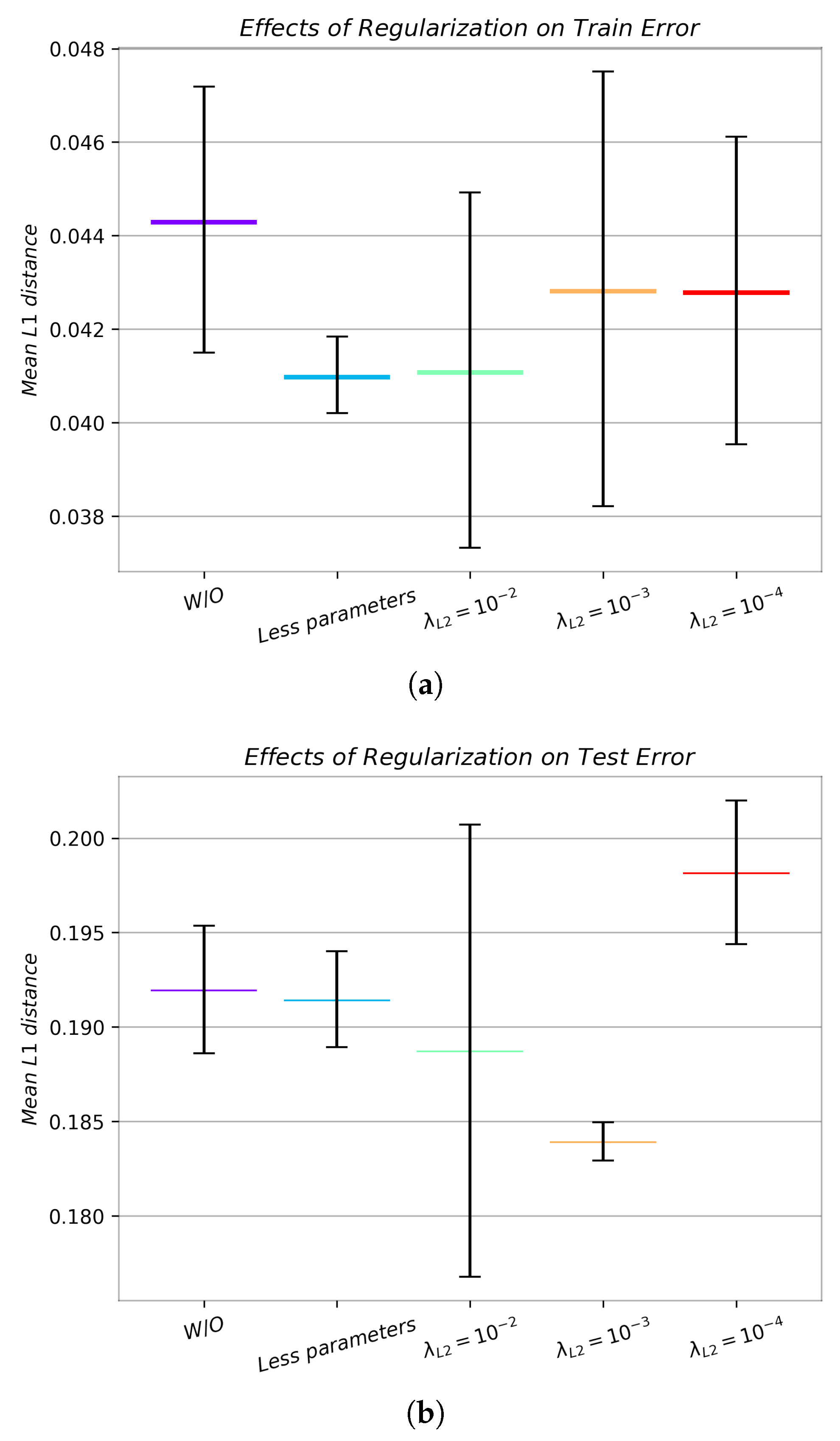
In an effort to combat the shortcomings of our main approach, and in the interest of demonstrating its true capabilities, we apply several regularization techniques to increase the validation and test accuracy of the pix2pix, thus reducing the variance of the model. We present our results after separately applying two different regularization techniques, described in Section 2.4, and varying their hyperparameters, in Figure 12 and Table 2. We observe various degrees of success.
The L2 regularization technique for the most part successfully reduces the validation/test error and improves accuracy. We observe faster convergence to plausible and relatively crisp results, and somewhat slower convergence to the errors achieved by the original architecture, implying that, indeed, the original architecture is superfluous given the magnitude of data we are able to effectively use.
As a whole, we observe that regularization techniques that were unnecessary in [55] do actually produce some promising results. The reason we examine these specific techniques, however, other than they are computationally less laborious to implement and stabilize, is that, according to several large-scale contemporary studies of regularization and consolidation of GANs [75,76,77], it is evident that more elaborate techniques are necessary to achieve better results while using GANs, while in [78], it is reported that an unregularized GAN yields better results that one regularized with L2 Regularization. Moreover, the current dogma in DL is to build deep and complex architectures and utilize regularization to avoid overfitting, and reducing the number of parameters is usually deterred and avoided.
To summarize, given that we have successfully demonstrated that regularization techniques inappropriate for GANs have successfully increased or at least not hurt performance, along with the performance on the training data, we have palpable evidence which suggest that the less-than-optimal performance of the original architecture can be attributed to the paucity of data and better generalization is to be expected. Note that our data augmentation method, albeit it provides a significant boost in performance, cannot be solely relied on to optimally solve the problem of overfitting. In fact, most of the contribution of data augmentation can be traced in allowing the generator to fool the discriminator in unseen test examples rather than reducing the L1 metric.
3.3. Inverse Problem and Generator
Given that DL algorithms are task agnostic, meaning that one can readily extend an algorithm or a model to accommodate another task, albeit some limitations exist, we can use the very same techniques to study the inverse problem, i.e., train the inverse operator, , to predict the surface coloration, meaning the RGB image, conditioned on a DEM. Note that simply “inverting” the generator G is not an option, as it is NP-hard to do so [79]. This generator is useful in itself, with applications like automated terrain generation (see Figure 13), but it is also useful as a regularization technique for our original generator. In more detail, several works [57,80] have deployed the inverse generator to force the original generator to preserve enough semantic information during the mapping between one domain to the other-in our case, from remotely sensed imagery to DEMs-so as to render the result informative enough for the inverse generator to be able to reconstruct the original input from it. In other words, we can use the generated DEM as input to the inverse generator and task it with mapping it to the original observation space, its corresponding remotely sensed image. We comment on the performance of such a technique, similar to the one presented in [57], in comparison to pix2pix and other baselines in Section 3.4.
3.4. Baselines
To demonstrate the efficacy of pix2pix, we compare its performance to two baselines, the plain U-net and CycleGAN. Our main goal is to justify our choice of generator-discriminator framework by comparing it to a strong CGAN baseline and demonstarting that a CNN augmented by the CGAN framework produces better results that a plain CNN by comparing pix2pix to the plain U-net.
3.4.1. CycleGAN
The CycleGAN architecture, as described in its original study and briefly alluded to in Section 3.3, is meant for unsupervised learning of meaningful bijections and was observed to perform better at such problems. However, due to the fact that we study an elaborate supervised learning task, we add to the original CycleGAN loss the pixel-wise L1 loss of the output of each generator,
where X is the domain of remotely sensed imagery, Y that of DEMs, G the original generator, and the inverse generator. We set and otherwise keep . This transforms the objective into a supervised one. The loss succinctly delineates the function of CycleGAN. We also deviate from the original paper in using the U-net to model the generators. Due to memory and resource constraints, it is unfortunately not possible for us to test generators of the same magnitude as pix2pix, as the generator is the costliest part of the procedure, as it ought to be, and we cannot support another model of similar magnitude. So, we test and compare with an architecture with sufficiently small generators. Even with our modifications to better guide training, we cannot get the networks to converge on a meaningful solution, probably due to the added complexity which allows the model to deviate from its original purpose and exert some of its capacity in preserving details for the input image reconstruction, along, of course, with the diminution of the number of parameters, which, as studied in Section 3.2, cannot be solely accountable for the deterioration in performance. Also, note that while training the inverse generator, predicting RGB images from DEMs, due to the increased degrees of freedom that this problem allows for, we noticed mode collapses and some moderate difficulty in convergence. The reconstructions presented in Figure 14 are indicative.
3.4.2. U-net
We also test the U-net, a staple in remote sensing, as remotely sensed imagery and DEMs have the same high-level structure. This could as well be an ablation study, as the U-net is, in effect, the generator used in every test in our work. However, its prevalence, along with the prevalence of traditional CNN architectures in remote sensing, renders it more appropriate as a baseline. We do not deviate in the number of parameters either, essaying to present as fair a comparison as possible. The advantage of pix2pix is clear, as presented in Figure 14. The deterioration of the qualitative performance can be attributed to the training framework, as it is the sole difference between this baseline and our chosen model. Our results demonstrate the ability of the GAN framework to guide the training of the U-net so as to maximally utilize its capacity instead of collapsing to the easy but unsatisfactory solution of smoothing the surface and producing its envelope or a local average in an effort to minimize error, remaining unable to capture the underlying structure. Similar effects are observed in [82].
4. Discussion
The idea of interpreting patterns in remotely sensed imagery to reconstruct the 3D geometry of a landscape is one of the most common fields of remote sensing known as photogrammetry. This method of acquiring high resolution 3D coordinates of objects requires a range of densely overlapping images and an image registration algorithm to align those images correctly. This range of images is granted by costly techniques like Lidar or other scanning methods. Our approach essays to overcome this obstacle, by using a single image as input to predict a plausible 3D representation of its surface, using a CGAN architecture. We observe that CGANs built for supervised tasks can begin to better approximate the true distribution of DEMs conditioned on remotely sensed images, providing realistic textures, compared to the other tested baselines, even with a paucity of data. Moreover, notice the difference in quality of the results between the Figure 8 and Figure 9, Figure 14, where data augmentation is used and not used respectively. These results, along with large-scale studies [83,84,85], suggest that, given the right amount of data and resources, CGANs can become a reliable tool in extracting 3D geometry from remotely sensed imagery. So, for our generative model to be successful at learning a correct mapping from remotely sensed images to elevation models, a high demand of data is required. Obviously, the capability of producing high quality 3D landscape predictions can be used, as is, in numerous applications of varying nature as aforementioned. Moreover, providing knowledge of a 3D point cloud description of the landscape as supplemental data to other DL models, working on remote sensing problems, has been proven to improve accuracy and the ability to generalize learned knowledge with greater accuracy on validation data [86]. Thus, such a model can be effective as a fully differentiable submodule in any other application. In fact, preliminary results in an urban image segmentation task where DSMs were unavailable during training and testing, predicting these DSMs with our proposed approach, trained in a nearby area, resulted in roughly 1% increase in the accuracy of the segmentation with no particular finetuning.
An issue that arises is that datasets of satellite or drone images and their corresponding DEMs are constructed by photogrammetric techniques. Consequently, the model learns the distribution of the output of such techniques rather than the “real-world” distribution of DEMs. However, in Figure 10, we observe that the ground truth DEMs can contain glaring inconsistencies, whereas the DL model seems to yield a more appropriate result. While this sample is not used during training but solely for evaluation, more such examples are expected to exist in the training sets, indicating that the model does not converge to pathological solutions nor does it “blindly” memorizes the training set. Another problem that can arise pertains the consistency of the color bands [87]. Even though that is an important issue, slight perturbations in the color of an image that may significantly alter the output of a network is a fundamental subject of study for the field of Adversarial Robustness [88,89,90] and therefore beyond the scope of this study and is left for future work.
Evaluating a generative model is an open and very difficult problem to solve. The same applies to comparing the performance of different architectures on the same problem. The essential problem is the absence of an error metric that describes if a generated image is a correct and realistic representation of the target domain of elevation models conditioned on the input image. If such a metric existed, it would be used in the loss function and, therefore, the model would be infallible after repeatedly iterating over the dataset during the training process. Traditional metrics such as Mean Square Error and L1 error, are not capable of measuring if a generated result captures the requested structure. Therefore, we mostly rely on human observation to evaluate our results.
It is also important to reiterate that, presumably due to resource constraints as we attempt to prove, the quantitative performance of our examined models cannot begin to compare with contemporary techniques. We view this shortcoming as an inevitable pitfall in the first attempt to solve this problem using solely AI and ML. More progress and more data is sure to ameliorate performance. Additionally, much research is carried out in 3D depth estimation [41,91,92] and specialized architectures are starting to emerge.
Evidently, due to the nature of the elevation data we are trying to predict, it is extremely challenging to capture the exact altitude of the objects existing in the image. It is more feasible to predict a representation of relative elevation points that accurately describes a three dimensional translation of the image provided. The empirical reason for this is that predicting the exact height map from an input image, is a very complex task to solve, as those values are computed on a global basis but only a local tile of information is provided. A more practical explanation, is that for CGANs to converge correctly and to be trained efficiently, the data fed to the network, must be normalized to a floating point range. Training on unbounded inputs would require vast amounts of data. Therefore, normalization is applied and the results are expected to be in the same range of values. To get to the true height values, knowledge of the true minimum and maximum altitude values of the validation data would be obligatory to rescale the predicted values to that range. That, naturally, limits the range of possible heights the model can predict.
5. Conclusions
In this work, we consider the problem of generating the Digital Elevation Model (DEM) of any given landscape. We model landscapes by their corresponding RGB remotely sensed images, and the relation between the two domains as an image-to-image translation function. We thoroughly examine novel end-to-end approaches to train a generator to approximate this function with state-of-the-art Deep Learning techniques, Conditional Generative Adversarial Networks (CGAN), to produce a DEM conditioned only on its corresponding RGB remotely sensed image. We validate the efficacy of the models mostly qualitatively but also quantitatively. We observe that [55] can truly begin to capture the underlying relation between remotely sensed imagery and DEMs compared to the other examined methods. It can yield plausible results on unseen data and can capture the intricate structure of surface elevation, producing sharp and complex textures, compared to the other methods that fail to do so. Our results demonstrate the ability of the CGAN framework to guide the training of the U-net [45] so as to maximally utilize its capacity instead of collapsing to the easy but unsatisfactory solution of smoothing the surface and producing its approximate envelope or a local average in order to minimize error, ultimately not capturing the underlying structure. Our method does not outperform other contemporary methods at the moment, but requires only a fraction of the data to operate once trained. Moreover, we show palpable evidence that the paucity of data is to blame for the decent but suboptimal generalization error and future work should be able to readily address this issue. Using an unbounded activation function in the final layer of the generator also constitutes a necessary development for the architecture so it can be deployed in useful applications, so that heights outside the range of the training dataset can be predicted.
Author Contributions
Conceptualization, E.P.; Data curation, E.P. and L.G.; Formal analysis, G.C.; Investigation, E.P. and G.C.; Methodology, E.P., G.C. and E.C.; Project administration, E.C.; Resources, E.P. and G.C.; Software, E.P. and G.C.; Supervision, E.C.; Validation, E.P., G.C., L.G. and E.C.; Visualization, E.P., G.C. and L.G.; Writing—original draft, E.P., G.C. and E.C.; Writing—review & editing, G.C. and Lazaros Grammatikopoulos. All authors have read and agreed to the published version of the manuscript.
Funding
This research received no external funding.
Conflicts of Interest
The authors declare no conflict of interest.
References
- Walker, J.P.; Willgoose, G.R. On the effect of digital elevation model accuracy on hydrology and geomorphology. Water Resour. Res. 1999, 35, 2259–2268. [Google Scholar] [CrossRef] [Green Version]
- Hancock, G.R. The use of digital elevation models in the identification and characterization of catchments over different grid scales. Hydrol. Process. Int. J. 2005, 19, 1727–1749. [Google Scholar] [CrossRef]
- Jaboyedoff, M.; Baillifard, F.; Couture, R.; Locat, J.; Locat, P. New insight of geomorphology and landslide prone area detection using digital elevation model (s). In Landslides: Evaluation and Stabilization; Balkema, Taylor & Francis Group: London, UK, 2004; pp. 191–198. [Google Scholar]
- Kenward, T.; Lettenmaier, D.P.; Wood, E.F.; Fielding, E. Effects of digital elevation model accuracy on hydrologic predictions. Remote Sens. Environ. 2000, 74, 432–444. [Google Scholar] [CrossRef]
- Wang, M.; Hjelmfelt, A.T. DEM based overland flow routing model. J. Hydrol. Eng. 1998, 3, 1–8. [Google Scholar] [CrossRef]
- Kharchenko, V.; Kuzmenko, N. Unmanned aerial vehicle collision avoidance using digital elevation model. Proc. Natl. Aviat. Univ. 2013, 1, 21–25. [Google Scholar] [CrossRef]
- Uijt_de_Haag, M.; Vadlamani, A. Flight test evaluation of various terrain referenced navigation techniques for aircraft approach guidance. In Proceedings of the 2006 IEEE/ION Position, Location, and Navigation Symposium, Coronado, CA, USA, 25–27 April 2006; pp. 440–449. [Google Scholar]
- Jenson, S.K.; Domingue, J.O. Extracting topographic structure from digital elevation data for geographic information system analysis. Photogramm. Eng. Remote Sens. 1988, 54, 1593–1600. [Google Scholar]
- Costa, E. Simulation of the effects of different urban environments on GPS performance using digital elevation models and building databases. IEEE Trans. Intell. Transp. Syst. 2011, 12, 819–829. [Google Scholar] [CrossRef]
- Hofmann-Wellenhof, B.; Lichtenegger, H.; Wasle, E. GNSS–Global Navigation Satellite Systems: GPS, GLONASS, Galileo, and More; Springer Science & Business Media: Berlin, Germany, 2007. [Google Scholar]
- Mercer, B.; Zhang, Q. Recent advances in airborne InSAR for 3D applications. In International Archives of the Photogrammetry, Remote Sensing and Spatial Information Sciences; ISPRS: Beijing, China, 2008; Volume XXXVII, Part B1; pp. 141–146. [Google Scholar]
- Quddus, M.A.; Zheng, Y. Low-Cost Tightly Coupled GPS, Dead-Reckoning, and Digital Elevation Model Land Vehicle Tracking System for Intelligent Transportation Systems; Technical Report; Transportation Research Board: Washington, DC, USA, 2011. [Google Scholar]
- Kaul, M.; Yang, B.; Jensen, C.S. Building accurate 3d spatial networks to enable next generation intelligent transportation systems. In Proceedings of the 2013 IEEE 14th International Conference on Mobile Data Management, Milan, Italy, 3–6 June 2013; Volume 1, pp. 137–146. [Google Scholar]
- Senay, G.B.; Ward, A.D.; Lyon, J.G.; Fausey, N.R.; Nokes, S.E. Manipulation of high spatial resolution aircraft remote sensing data for use in site-specific farming. Trans. ASAE 1998, 41, 489. [Google Scholar] [CrossRef]
- Lu, Y.C.; Daughtry, C.; Hart, G.; Watkins, B. The current state of precision farming. Food Rev. Int. 1997, 13, 141–162. [Google Scholar] [CrossRef]
- Grammatikopoulos, L.; Adam, K.; Petsa, E.; Karras, G. Camera Calibation using Multiple Unordered Coplanar Chessboards. Int. Arch. Photogramm. Remote Sens. Spat. Inf. Sci. 2019, 42, 59–66. [Google Scholar] [CrossRef] [Green Version]
- Leitão, J.P.; de Vitry, M.M.; Scheidegger, A.; Rieckermann, J. Assessing the quality of digital elevation models obtained from mini unmanned aerial vehicles for overland flow modelling in urban areas. Hydrol. Earth Syst. Sci. 2016, 20, 1637. [Google Scholar] [CrossRef] [Green Version]
- Ruiz, J.; Diaz-Mas, L.; Perez, F.; Viguria, A. Evaluating the accuracy of DEM generation algorithms from UAV imagery. Int. Arch. Photogramm. Remote Sens. Spat. Inf. Sci 2013, 40, 333–337. [Google Scholar] [CrossRef]
- Baselice, F.; Ferraioli, G.; Pascazio, V.; Schirinzi, G. Contextual information-based multichannel synthetic aperture radar interferometry: Addressing DEM reconstruction using contextual information. IEEE Signal Process. Mag. 2014, 31, 59–68. [Google Scholar] [CrossRef]
- Devlin, J.; Chang, M.W.; Lee, K.; Toutanova, K. Bert: Pre-training of deep bidirectional transformers for language understanding. arXiv 2018, arXiv:1810.04805. [Google Scholar]
- Seide, F.; Li, G.; Yu, D. Conversational speech transcription using context-dependent deep neural networks. In Proceedings of the Twelfth Annual Conference of the International Speech Communication Association, Florence, Italy, 27–31 August 2011. [Google Scholar]
- Iandola, F.N.; Han, S.; Moskewicz, M.W.; Ashraf, K.; Dally, W.J.; Keutzer, K. SqueezeNet: AlexNet-level accuracy with 50x fewer parameters and <0.5 MB model size. arXiv 2016, arXiv:1602.07360. [Google Scholar]
- Krizhevsky, A.; Sutskever, I.; Hinton, G.E. Imagenet classification with deep convolutional neural networks. In Advances in Neural Information Processing Systems; Curran Associates, Inc.: Red Hook, NY, USA, 2012; pp. 1097–1105. [Google Scholar]
- Szegedy, C.; Liu, W.; Jia, Y.; Sermanet, P.; Reed, S.; Anguelov, D.; Erhan, D.; Vanhoucke, V.; Rabinovich, A. Going deeper with convolutions. In Proceedings of the IEEE Conference on Computer Vision and Pattern Recognition, Boston, MA, USA, 7–12 June 2015; pp. 1–9. [Google Scholar]
- Mnih, V.; Kavukcuoglu, K.; Silver, D.; Graves, A.; Antonoglou, I.; Wierstra, D.; Riedmiller, M. Playing atari with deep reinforcement learning. arXiv 2013, arXiv:1312.5602. [Google Scholar]
- Mnih, V.; Kavukcuoglu, K.; Silver, D.; Rusu, A.A.; Veness, J.; Bellemare, M.G.; Graves, A.; Riedmiller, M.; Fidjeland, A.K.; Ostrovski, G.; et al. Human-level control through deep reinforcement learning. Nature 2015, 518, 529–533. [Google Scholar] [CrossRef]
- He, K.; Zhang, X.; Ren, S.; Sun, J. Delving deep into rectifiers: Surpassing human-level performance on imagenet classification. In Proceedings of the IEEE International Conference on Computer Vision, Santiago, Chile, 7–13 December 2015; pp. 1026–1034. [Google Scholar]
- Silver, D.; Hubert, T.; Schrittwieser, J.; Antonoglou, I.; Lai, M.; Guez, A.; Lanctot, M.; Sifre, L.; Kumaran, D.; Graepel, T.; et al. Mastering Chess and Shogi by Self-Play with a General Reinforcement Learning Algorithm. arXiv 2017, arXiv:cs.AI/1712.01815. [Google Scholar]
- Ma, L.; Liu, Y.; Zhang, X.; Ye, Y.; Yin, G.; Johnson, B.A. Deep learning in remote sensing applications: A meta-analysis and review. ISPRS J. Photogramm. Remote Sens. 2019, 152, 166–177. [Google Scholar] [CrossRef]
- Zhu, X.X.; Tuia, D.; Mou, L.; Xia, G.S.; Zhang, L.; Xu, F.; Fraundorfer, F. Deep learning in remote sensing: A comprehensive review and list of resources. IEEE Geosci. Remote Sens. Mag. 2017, 5, 8–36. [Google Scholar] [CrossRef] [Green Version]
- Zhang, L.; Zhang, L.; Du, B. Deep learning for remote sensing data: A technical tutorial on the state of the art. IEEE Geosci. Remote Sens. Mag. 2016, 4, 22–40. [Google Scholar] [CrossRef]
- Ball, J.E.; Anderson, D.T.; Chan, C.S. Comprehensive survey of deep learning in remote sensing: Theories, tools, and challenges for the community. J. Appl. Remote Sens. 2017, 11, 042609. [Google Scholar] [CrossRef] [Green Version]
- Kussul, N.; Lavreniuk, M.; Skakun, S.; Shelestov, A. Deep learning classification of land cover and crop types using remote sensing data. IEEE Geosci. Remote Sens. Lett. 2017, 14, 778–782. [Google Scholar] [CrossRef]
- Zou, Q.; Ni, L.; Zhang, T.; Wang, Q. Deep learning based feature selection for remote sensing scene classification. IEEE Geosci. Remote Sens. Lett. 2015, 12, 2321–2325. [Google Scholar] [CrossRef]
- Charou, E.; Felekis, G.; Stavroulopoulou, D.B.; Koutsoukou, M.; Panagiotopoulou, A.; Voutos, Y.; Bratsolis, E.; Mylonas, P.; Likforman-Sulem, L. Deep Learning for Agricultural Land Detection in Insular Areas. In Proceedings of the 2019 10th International Conference on Information, Intelligence, Systems and Applications (IISA), Patras, Greece, 15–17 July 2019; pp. 1–4. [Google Scholar]
- Lanaras, C.; Bioucas-Dias, J.; Galliani, S.; Baltsavias, E.; Schindler, K. Super-resolution of Sentinel-2 images: Learning a globally applicable deep neural network. ISPRS J. Photogramm. Remote Sens. 2018, 146, 305–319. [Google Scholar] [CrossRef] [Green Version]
- Yuan, Y.; Zheng, X.; Lu, X. Hyperspectral image superresolution by transfer learning. IEEE J. Sel. Top. Appl. Earth Obs. Remote Sens. 2017, 10, 1963–1974. [Google Scholar] [CrossRef]
- Torres, R.N.; Fraternali, P.; Milani, F.; Frajberg, D. A Deep Learning model for identifying mountain summits in Digital Elevation Model data. In Proceedings of the 2018 IEEE First International Conference on Artificial Intelligence and Knowledge Engineering (AIKE), Laguna Hills, CA, USA, 26–28 September 2018; pp. 212–217. [Google Scholar]
- Marmanis, D.; Adam, F.; Datcu, M.; Esch, T.; Stilla, U. Deep neural networks for above-ground detection in very high spatial resolution digital elevation models. ISPRS Ann. Photogramm. Remote Sens. Spat. Inf. Sci. 2015, 2, 103. [Google Scholar] [CrossRef] [Green Version]
- Kulp, S.A.; Strauss, B.H. CoastalDEM: A global coastal digital elevation model improved from SRTM using a neural network. Remote Sens. Environ. 2018, 206, 231–239. [Google Scholar] [CrossRef]
- Mou, L.; Zhu, X.X. IM2HEIGHT: Height estimation from single monocular imagery via fully residual convolutional-deconvolutional network. arXiv 2018, arXiv:1802.10249. [Google Scholar]
- Godard, C.; Mac Aodha, O.; Firman, M.; Brostow, G.J. Digging into self-supervised monocular depth estimation. In Proceedings of the IEEE International Conference on Computer Vision, Seoul, Korea, 27 October–2 November 2019; pp. 3828–3838. [Google Scholar]
- Zhou, T.; Brown, M.; Snavely, N.; Lowe, D.G. Unsupervised learning of depth and ego-motion from video. In Proceedings of the IEEE Conference on Computer Vision and Pattern Recognition, Honolulu, HI, USA, 21–26 July 2017; pp. 1851–1858. [Google Scholar]
- Abrevaya, V.F.; Boukhayma, A.; Torr, P.H.; Boyer, E. Cross-modal Deep Face Normals with Deactivable Skip Connections. arXiv 2020, arXiv:2003.09691. [Google Scholar]
- Ronneberger, O.; Fischer, P.; Brox, T. U-net: Convolutional networks for biomedical image segmentation. In Proceedings of the International Conference on Medical Image Computing and Computer-Assisted Intervention, Munich, Germany, 5–9 October 2015; Springer: Berlin, Germany, 2015; pp. 234–241. [Google Scholar]
- He, K.; Zhang, X.; Ren, S.; Sun, J. Deep residual learning for image recognition. In Proceedings of the IEEE Conference on Computer Vision and Pattern Recognition, Las Vegas, NV, USA, 27–30 June 2016; pp. 770–778. [Google Scholar]
- Goodfellow, I.; Bengio, Y.; Courville, A. Deep Learning; MIT Press: Cambridge, MA, USA, 2016; Available online: http://www.deeplearningbook.org (accessed on 12 June 2020).
- Goodfellow, I.; Pouget-Abadie, J.; Mirza, M.; Xu, B.; Warde-Farley, D.; Ozair, S.; Courville, A.; Bengio, Y. Generative adversarial nets. In Proceedings of the Advances in Neural Information Processing Systems, Montreal, QC, Canada, 8–13 December 2014; pp. 2672–2680. [Google Scholar]
- Mirza, M.; Osindero, S. Conditional generative adversarial nets. arXiv 2014, arXiv:1411.1784. [Google Scholar]
- Reed, S.; Akata, Z.; Yan, X.; Logeswaran, L.; Schiele, B.; Lee, H. Generative adversarial text to image synthesis. arXiv 2016, arXiv:1605.05396. [Google Scholar]
- Zhang, H.; Xu, T.; Li, H.; Zhang, S.; Wang, X.; Huang, X.; Metaxas, D.N. Stackgan: Text to photo-realistic image synthesis with stacked generative adversarial networks. In Proceedings of the IEEE International Conference on Computer Vision, Venice, Italy, 22–29 October 2017; pp. 5907–5915. [Google Scholar]
- Zhang, H.; Xu, T.; Li, H.; Zhang, S.; Wang, X.; Huang, X.; Metaxas, D.N. Stackgan++: Realistic image synthesis with stacked generative adversarial networks. IEEE Trans. Pattern Anal. Mach. Intell. 2018, 41, 1947–1962. [Google Scholar] [CrossRef] [Green Version]
- Higgins, I.; Matthey, L.; Glorot, X.; Pal, A.; Uria, B.; Blundell, C.; Mohamed, S.; Lerchner, A. Early visual concept learning with unsupervised deep learning. arXiv 2016, arXiv:1606.05579. [Google Scholar]
- Rawat, W.; Wang, Z. Deep convolutional neural networks for image classification: A comprehensive review. Neural Comput. 2017, 29, 2352–2449. [Google Scholar] [CrossRef]
- Isola, P.; Zhu, J.Y.; Zhou, T.; Efros, A.A. Image-to-image translation with conditional adversarial networks. In Proceedings of the IEEE Conference on Computer Vision and Pattern Recognition, Honolulu, HI, USA, 21–26 July 2017; pp. 1125–1134. [Google Scholar]
- Zhu, X.; Li, Z.; Zhang, X.; Li, H.; Xue, Z.; Wang, L. Generative Adversarial Image Super-Resolution through Deep Dense Skip Connections; Computer Graphics Forum; Wiley Online Library: Hoboken, NJ, USA, 2018; Volume 37, pp. 289–300. [Google Scholar]
- Zhu, J.Y.; Park, T.; Isola, P.; Efros, A.A. Unpaired image-to-image translation using cycle-consistent adversarial networks. In Proceedings of the IEEE international Conference on Computer Vision, Venice, Italy, 22–29 October 2017; pp. 2223–2232. [Google Scholar]
- Ioffe, S.; Szegedy, C. Batch normalization: Accelerating deep network training by reducing internal covariate shift. arXiv 2015, arXiv:1502.03167. [Google Scholar]
- Xu, B.; Wang, N.; Chen, T.; Li, M. Empirical evaluation of rectified activations in convolutional network. arXiv 2015, arXiv:1505.00853. [Google Scholar]
- Kingma, D.P.; Ba, J. Adam: A method for stochastic optimization. arXiv 2014, arXiv:1412.6980. [Google Scholar]
- Srivastava, N.; Hinton, G.; Krizhevsky, A.; Sutskever, I.; Salakhutdinov, R. Dropout: A simple way to prevent neural networks from overfitting. J. Mach. Learn. Res. 2014, 15, 1929–1958. [Google Scholar]
- Abadi, M.; Barham, P.; Chen, J.; Chen, Z.; Davis, A.; Dean, J.; Devin, M.; Ghemawat, S.; Irving, G.; Isard, M.; et al. Tensorflow: A system for large-scale machine learning. In Proceedings of the 12th {USENIX} Symposium on Operating Systems Design and Implementation ({OSDI} 16), Savannah, GA, USA, 2–4 November 2016; pp. 265–283. [Google Scholar]
- JAXA-EORC. ALOS Global Digital Surface Model “ALOS World 3D-30 m” (AW3D30). 2016. Available online: http://www.eorc.jaxa.jp/ALOS/en/aw3d30/index.htm (accessed on 25 May 2020).
- Gorelick, N.; Hancher, M.; Dixon, M.; Ilyushchenko, S.; Thau, D.; Moore, R. Google Earth Engine: Planetary-scale geospatial analysis for everyone. Remote Sens. Environ. 2017, 202, 18–27. [Google Scholar] [CrossRef]
- Map Ltd. Available online: http://map4u.gr/ (accessed on 23 May 2020).
- Karras, T.; Aila, T.; Laine, S.; Lehtinen, J. Progressive growing of gans for improved quality, stability, and variation. arXiv 2017, arXiv:1710.10196. [Google Scholar]
- Arora, S.; Ge, R.; Liang, Y.; Ma, T.; Zhang, Y. Generalization and equilibrium in generative adversarial nets (gans). In Proceedings of the 34th International Conference on Machine Learning-Volume 70. JMLR. org, Sydney, NSW, Australia, 6–11 August 2017; pp. 224–232. [Google Scholar]
- Ghifary, M.; Kleijn, W.B.; Zhang, M.; Balduzzi, D.; Li, W. Deep reconstruction-classification networks for unsupervised domain adaptation. In Proceedings of the European Conference on Computer Vision, Amsterdam, The Netherlands, 11–14 October 2016; Springer: Berlin, Germany, 2016; pp. 597–613. [Google Scholar]
- Liu, M.Y.; Tuzel, O. Coupled generative adversarial networks. In Proceedings of the Advances in Neural Information Processing Systems, Barcelona, Spain, 5–10 December 2016; pp. 469–477. [Google Scholar]
- Cao, Z.; Long, M.; Wang, J.; Jordan, M.I. Partial transfer learning with selective adversarial networks. In Proceedings of the IEEE Conference on Computer Vision and Pattern Recognition, Salt Lake City, UT, USA, 18–22 June 2018; pp. 2724–2732. [Google Scholar]
- Sankaranarayanan, S.; Balaji, Y.; Castillo, C.D.; Chellappa, R. Generate to adapt: Aligning domains using generative adversarial networks. In Proceedings of the IEEE Conference on Computer Vision and Pattern Recognition, Salt Lake City, UT, USA, 18–22 June 2018; pp. 8503–8512. [Google Scholar]
- Long, M.; Cao, Z.; Wang, J.; Jordan, M.I. Conditional adversarial domain adaptation. In Proceedings of the Advances in Neural Information Processing Systems, Montreal, QC, Canada, 3–8 December 2018; pp. 1640–1650. [Google Scholar]
- Reed, S.; Akata, Z.; Lee, H.; Schiele, B. Learning deep representations of fine-grained visual descriptions. In Proceedings of the IEEE Conference on Computer Vision and Pattern Recognition, Las Vegas, NV, USA, 26 June–1 July 2016; pp. 49–58. [Google Scholar]
- Tzeng, E.; Hoffman, J.; Saenko, K.; Darrell, T. Adversarial discriminative domain adaptation. In Proceedings of the IEEE Conference on Computer Vision and Pattern Recognition, Honolulu, HI, USA, 21–26 July 2017; pp. 7167–7176. [Google Scholar]
- Roth, K.; Lucchi, A.; Nowozin, S.; Hofmann, T. Stabilizing training of generative adversarial networks through regularization. In Proceedings of the Advances in Neural Information Processing Systems, Long Beach, CA, USA, 4–9 December 2017; pp. 2018–2028. [Google Scholar]
- Zhao, Z.; Singh, S.; Lee, H.; Zhang, Z.; Odena, A.; Zhang, H. Improved consistency regularization for gans. arXiv 2020, arXiv:2002.04724. [Google Scholar]
- Zhang, H.; Zhang, Z.; Odena, A.; Lee, H. Consistency Regularization for Generative Adversarial Networks. arXiv 2019, arXiv:1910.12027. [Google Scholar]
- Kurach, K.; Lucic, M.; Zhai, X.; Michalski, M.; Gelly, S. A large-scale study on regularization and normalization in GANs. arXiv 2018, arXiv:1807.04720. [Google Scholar]
- Lei, Q.; Jalal, A.; Dhillon, I.S.; Dimakis, A.G. Inverting Deep Generative models, One layer at a time. In Proceedings of the Advances in Neural Information Processing Systems, Vancouver, BC, Canada, 8–14 December 2019; pp. 13910–13919. [Google Scholar]
- Hoffman, J.; Tzeng, E.; Park, T.; Zhu, J.Y.; Isola, P.; Saenko, K.; Efros, A.A.; Darrell, T. Cycada: Cycle-consistent adversarial domain adaptation. arXiv 2017, arXiv:1711.03213. [Google Scholar]
- Perlin, K. An image synthesizer. ACM Siggraph Comput. Graph. 1985, 19, 287–296. [Google Scholar] [CrossRef]
- Zhu, L.; Chen, Y.; Ghamisi, P.; Benediktsson, J.A. Generative adversarial networks for hyperspectral image classification. IEEE Trans. Geosci. Remote Sens. 2018, 56, 5046–5063. [Google Scholar] [CrossRef]
- Nuha, F.U. Training dataset reduction on generative adversarial network. Procedia Comput. Sci. 2018, 144, 133–139. [Google Scholar] [CrossRef]
- Belkin, M.; Hsu, D.; Ma, S.; Mandal, S. Reconciling modern machine-learning practice and the classical bias–variance trade-off. Proc. Natl. Acad. Sci. USA 2019, 116, 15849–15854. [Google Scholar] [CrossRef] [Green Version]
- Sun, C.; Shrivastava, A.; Singh, S.; Gupta, A. Revisiting unreasonable effectiveness of data in deep learning era. In Proceedings of the IEEE International Conference on Computer Vision, Venice, Italy, 22–29 October 2017; pp. 843–852. [Google Scholar]
- Vetrivel, A.; Gerke, M.; Kerle, N.; Nex, F.; Vosselman, G. Disaster damage detection through synergistic use of deep learning and 3D point cloud features derived from very high resolution oblique aerial images, and multiple-kernel-learning. ISPRS J. Photogramm. Remote Sens. 2018, 140, 45–59. [Google Scholar] [CrossRef]
- Li, Z.; Zhu, H.; Zhou, C.; Cao, L.; Zhong, Y.; Zeng, T.; Liu, J. A Color Consistency Processing Method for HY-1C Images of Antarctica. Remote Sens. 2020, 12, 1143. [Google Scholar] [CrossRef] [Green Version]
- Goodfellow, I.J.; Shlens, J.; Szegedy, C. Explaining and harnessing adversarial examples. arXiv 2014, arXiv:1412.6572. [Google Scholar]
- Kurakin, A.; Goodfellow, I.; Bengio, S. Adversarial examples in the physical world. arXiv 2016, arXiv:1607.02533. [Google Scholar]
- Carlini, N.; Athalye, A.; Papernot, N.; Brendel, W.; Rauber, J.; Tsipras, D.; Goodfellow, I.; Madry, A.; Kurakin, A. On evaluating adversarial robustness. arXiv 2019, arXiv:1902.06705. [Google Scholar]
- Godard, C.; Mac Aodha, O.; Brostow, G.J. Unsupervised monocular depth estimation with left-right consistency. In Proceedings of the IEEE Conference on Computer Vision and Pattern Recognition, Honolulu, HI, USA, 21–26 July 2017; pp. 270–279. [Google Scholar]
- Liu, F.; Shen, C.; Lin, G. Deep convolutional neural fields for depth estimation from a single image. In Proceedings of the IEEE Conference on Computer Vision and Pattern Recognition, Boston, MA, USA, 7–12 June 2015; pp. 5162–5170. [Google Scholar]
Figure 1.
The discriminator architecture of choice: PatchGAN [55]. The discriminator decides whether its input is from the true data distribution based on local information by concentrating on the fidelity of individual image patches.
Figure 1.
The discriminator architecture of choice: PatchGAN [55]. The discriminator decides whether its input is from the true data distribution based on local information by concentrating on the fidelity of individual image patches.

Figure 2.
The generator architecture of choice: U-net [45]. It consists of an encoder that downsamples the input image using convolutional blocks up until the bottleneck layer, where the high-level semantic features of the input reside (for an explicit demonstration, see [53]). Thereafter, deconvolutional blocks upsample the image to the desired dimensions. The skip connections, denoted by pointed arrows between corresponding layers of the encoder and the decoder, facilitate training by providing crucial lower-level information from the encoder to the decoder. Given that the input and the output have the same low-level structure, these low-level features serve as the canvas that guides the decoder in the generation of the final output.

Figure 3.
Flow chart of the satellite-imagery dataset collection process using the Google Earth Engine API. The outermost points of the georeferenced DEM are selected as the boundary for the GeoJSON Polygon, which when fed into the API returns the corresponding RGB satellite image.
Figure 3.
Flow chart of the satellite-imagery dataset collection process using the Google Earth Engine API. The outermost points of the georeferenced DEM are selected as the boundary for the GeoJSON Polygon, which when fed into the API returns the corresponding RGB satellite image.

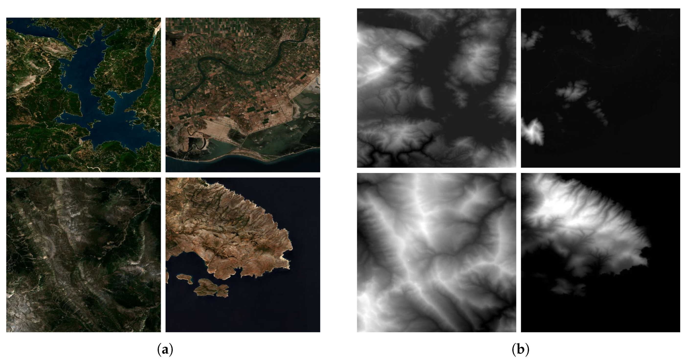
Figure 4.
Example (a) satellite images and (b) DEM tiles over different locations of Greece. The diversity of the landscape is apparent, highlighting the difficulty of the problem.
Figure 4.
Example (a) satellite images and (b) DEM tiles over different locations of Greece. The diversity of the landscape is apparent, highlighting the difficulty of the problem.

Figure 5.
An illustration of the 9-band input described at Table 1, presented from left to right and top to bottom. The higher variety in the input wavelengths provides auxiliary information for the DEM prediction.
Figure 5.
An illustration of the 9-band input described at Table 1, presented from left to right and top to bottom. The higher variety in the input wavelengths provides auxiliary information for the DEM prediction.

Figure 6.
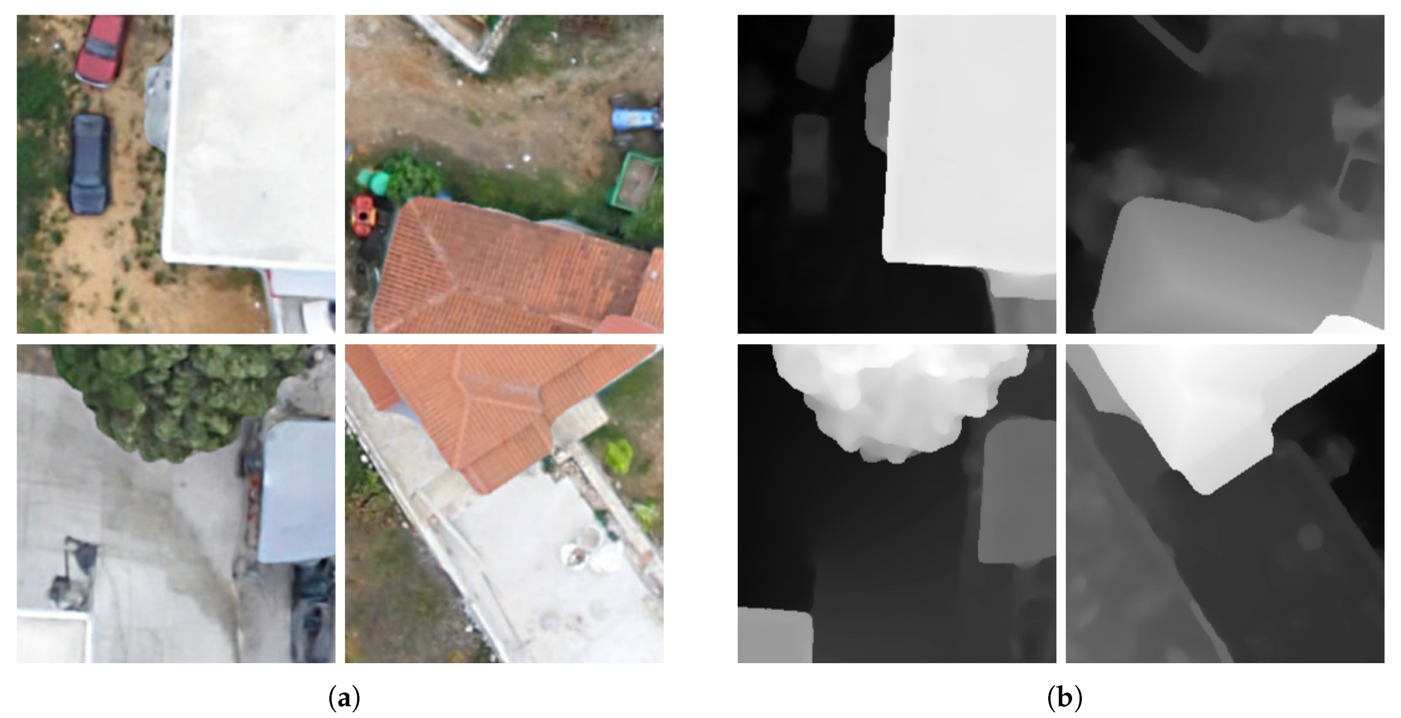
Urban dataset: Example (a) drone images and (b) DEM tiles taken over a Greek city. The target distribution is completely different compared to the satellite DEMs. The model will have to learn more complex structures such as trees, houses and cars.
Figure 6.
Urban dataset: Example (a) drone images and (b) DEM tiles taken over a Greek city. The target distribution is completely different compared to the satellite DEMs. The model will have to learn more complex structures such as trees, houses and cars.

Figure 7.
Rural dataset: Example (a) drone images and (b) DEM tiles taken over a Greek village. The target distribution is completely different compared to the satellite DEMs, but similar to the urban one (Figure 6).
Figure 7.
Rural dataset: Example (a) drone images and (b) DEM tiles taken over a Greek village. The target distribution is completely different compared to the satellite DEMs, but similar to the urban one (Figure 6).

Figure 8.
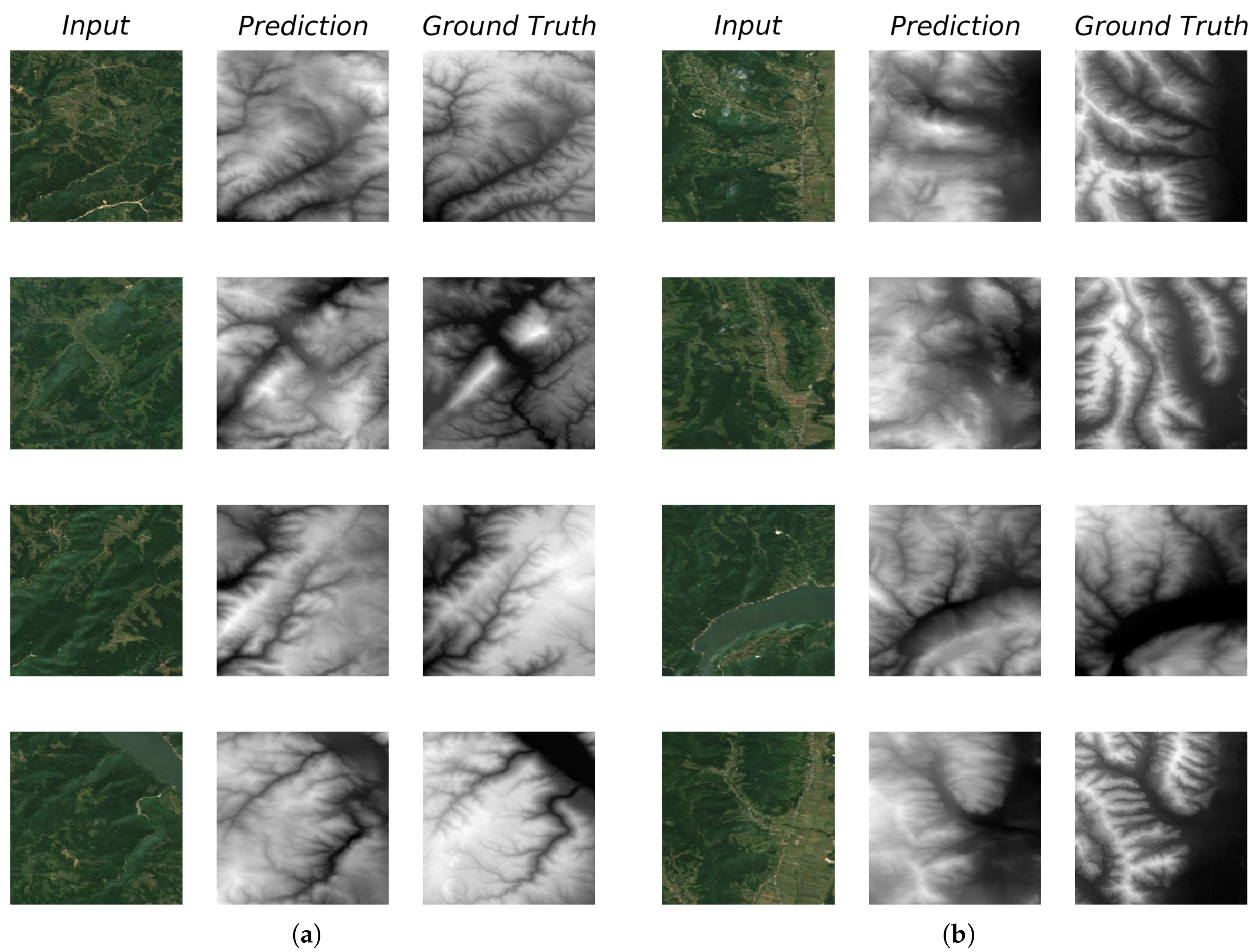
The generator’s results on previously unseen testing data. (a) In most cases it proves to have learned to capture the underlying relation between satellite imagery and DEMs, producing sharp results. (b) Even when reconstructions are poor, the model does not collapse to the easy solution of producing blurry results to approximate the result with minimum error, but manages to generate plausible representations in terms of DEM structure. Note that we used our data augmentation technique (Section 2.8).
Figure 8.
The generator’s results on previously unseen testing data. (a) In most cases it proves to have learned to capture the underlying relation between satellite imagery and DEMs, producing sharp results. (b) Even when reconstructions are poor, the model does not collapse to the easy solution of producing blurry results to approximate the result with minimum error, but manages to generate plausible representations in terms of DEM structure. Note that we used our data augmentation technique (Section 2.8).

Figure 9.
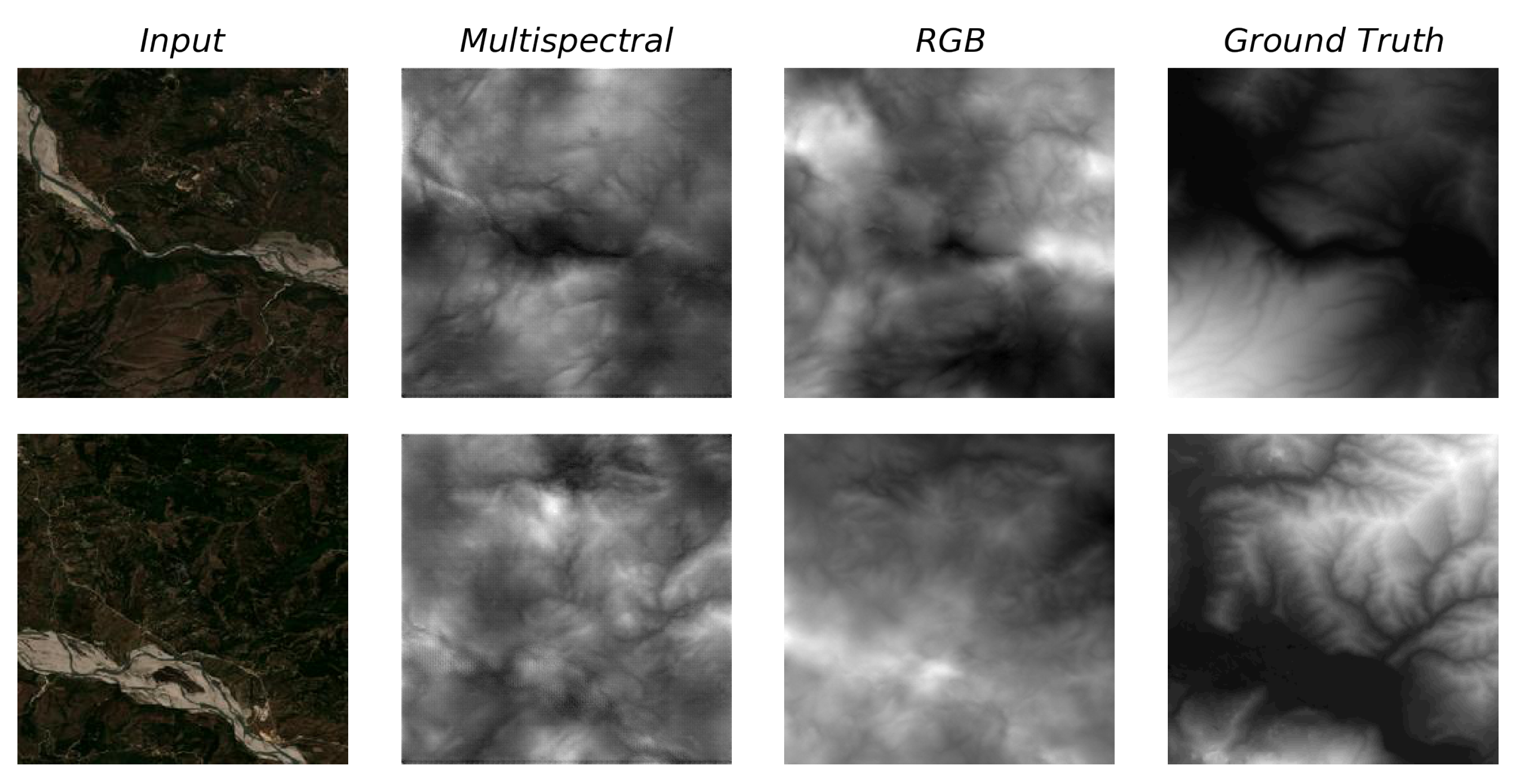
Some examples of the RGB model producing biased results, where river banks are treated as peaks. The model trained on multispectral dataset receives more enlightening information and partly corrects the artifact. Note that these models do not utilize data augmentation (Section 2.8), though we observe the same problem for the one trained as such on the RGB dataset.
Figure 9.
Some examples of the RGB model producing biased results, where river banks are treated as peaks. The model trained on multispectral dataset receives more enlightening information and partly corrects the artifact. Note that these models do not utilize data augmentation (Section 2.8), though we observe the same problem for the one trained as such on the RGB dataset.

Figure 10.
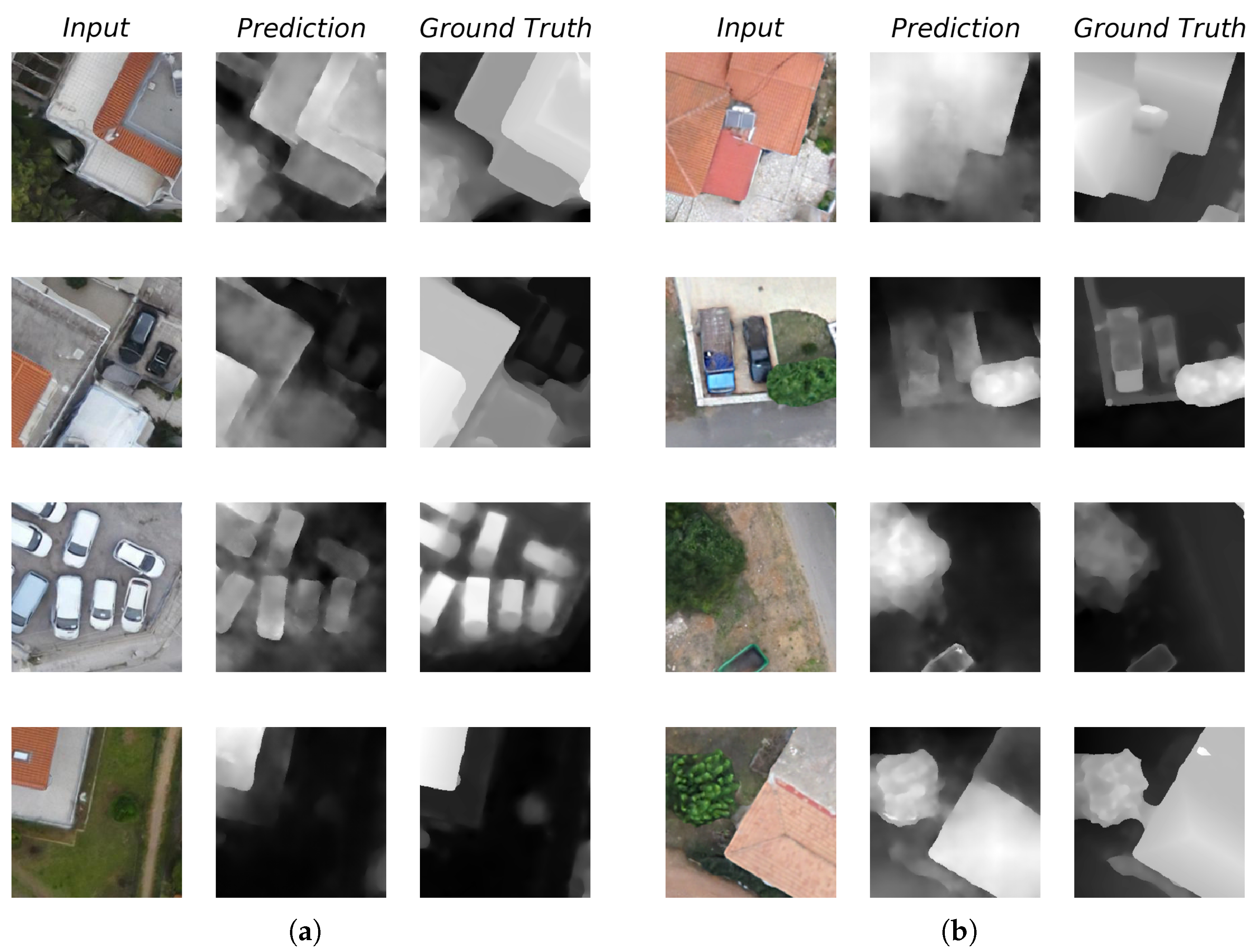
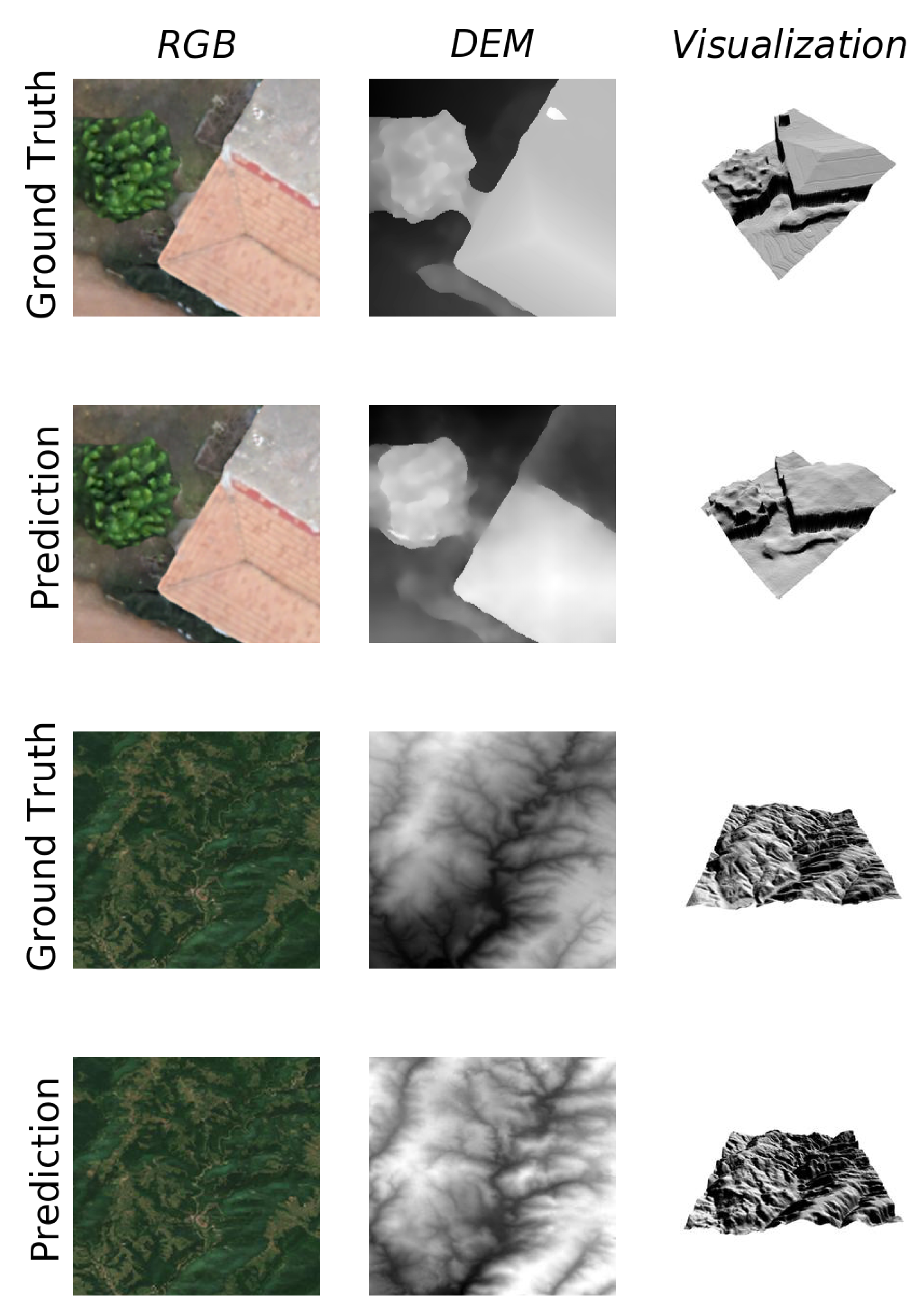
The generator’s results on previously unseen testing data of the (a) Urban and (b) Rural datasets. The model adequately captures the true data distribution, even though few examples are used during training. Notice that even though the ground truth DEM of the bottom row in (b) seems to contain an inaccuracy (the tree and the house appear connected), the generator’s prediction does not contain such an artifact.
Figure 10.
The generator’s results on previously unseen testing data of the (a) Urban and (b) Rural datasets. The model adequately captures the true data distribution, even though few examples are used during training. Notice that even though the ground truth DEM of the bottom row in (b) seems to contain an inaccuracy (the tree and the house appear connected), the generator’s prediction does not contain such an artifact.

Figure 11.
3D visualizations of the some predictions of pix2pix compared to the ground truths. The top two rows depict samples from the rural drone-borne dataset, while the last two from the satellite dataset. The input drone and satellite images are from the test set.
Figure 11.
3D visualizations of the some predictions of pix2pix compared to the ground truths. The top two rows depict samples from the rural drone-borne dataset, while the last two from the satellite dataset. The input drone and satellite images are from the test set.

Figure 12.
Quantitative effects of no regularization (W/O), L2 regularization () and diminished capacity (Less parameters) on train and test error of the normalized to satellite-imagery dataset. Absolute metrics can be seen in Table 2. All metrics represent distances in that range. Note that, due to resource constraints, we a priori reduce the capacity of all the models presented above, and no data augmentation (Section 2.8) is used. For more representative results of the unregularized model, refer to Figure 8. (a) We can see that, almost surprisingly, the training errors of the regularized models are on average better that the unregularized one, though all their ranges overlap. (b) We can observe statistically significant improvement of the error of some regularized models over the plain model. Note the large gap (variance) still in train and test performance, indicating overfitting. 2000 samples are used to calculate test error.

Figure 13.
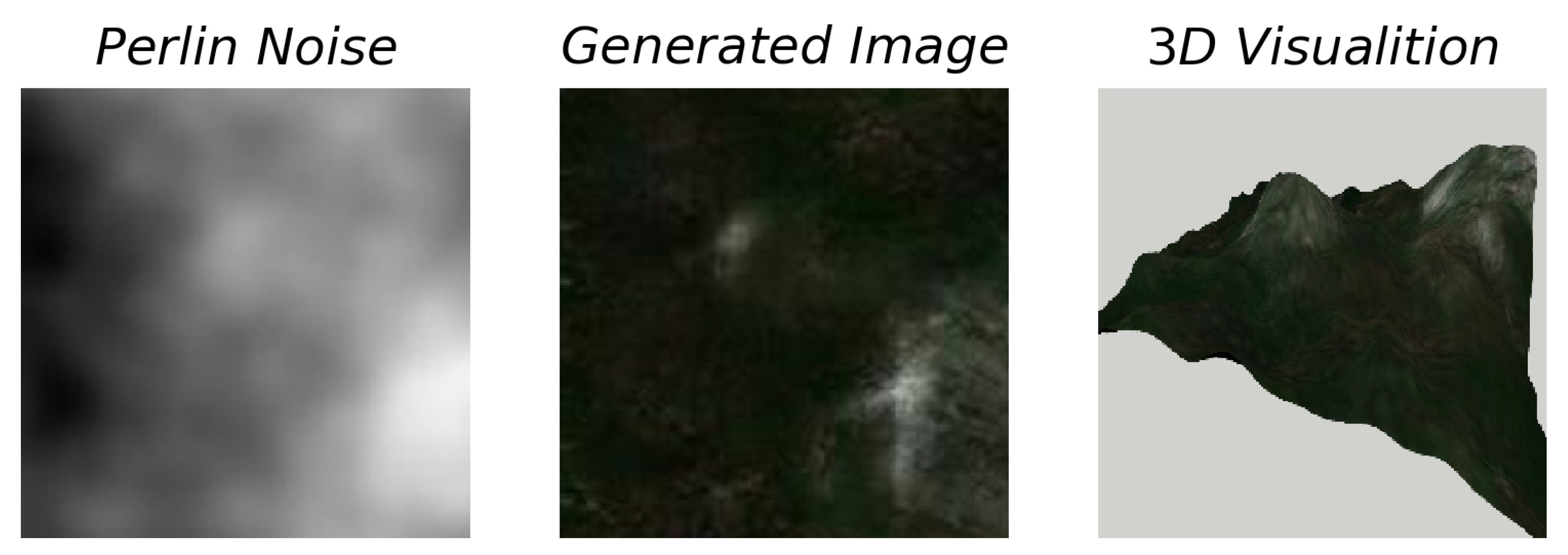
Given the inverse generator, , a model that produces RGB coloration conditioned on a DEM, on can artificially and automatically create and render plausible 3D environments. More precisely, we sample a DEM from a Perlin noise distribution [81], which is especially suited for generating plausible computer graphics imagery with peaks and valleys. By using this as input to the inverse generator, we are able to get a suitable coloration for it, yielding the above result. Provided this work does not study this problem, we have not optimized nor scrutinized the generator and present the result in the interest of demonstrating its applicability.
Figure 13.
Given the inverse generator, , a model that produces RGB coloration conditioned on a DEM, on can artificially and automatically create and render plausible 3D environments. More precisely, we sample a DEM from a Perlin noise distribution [81], which is especially suited for generating plausible computer graphics imagery with peaks and valleys. By using this as input to the inverse generator, we are able to get a suitable coloration for it, yielding the above result. Provided this work does not study this problem, we have not optimized nor scrutinized the generator and present the result in the interest of demonstrating its applicability.

Figure 14.
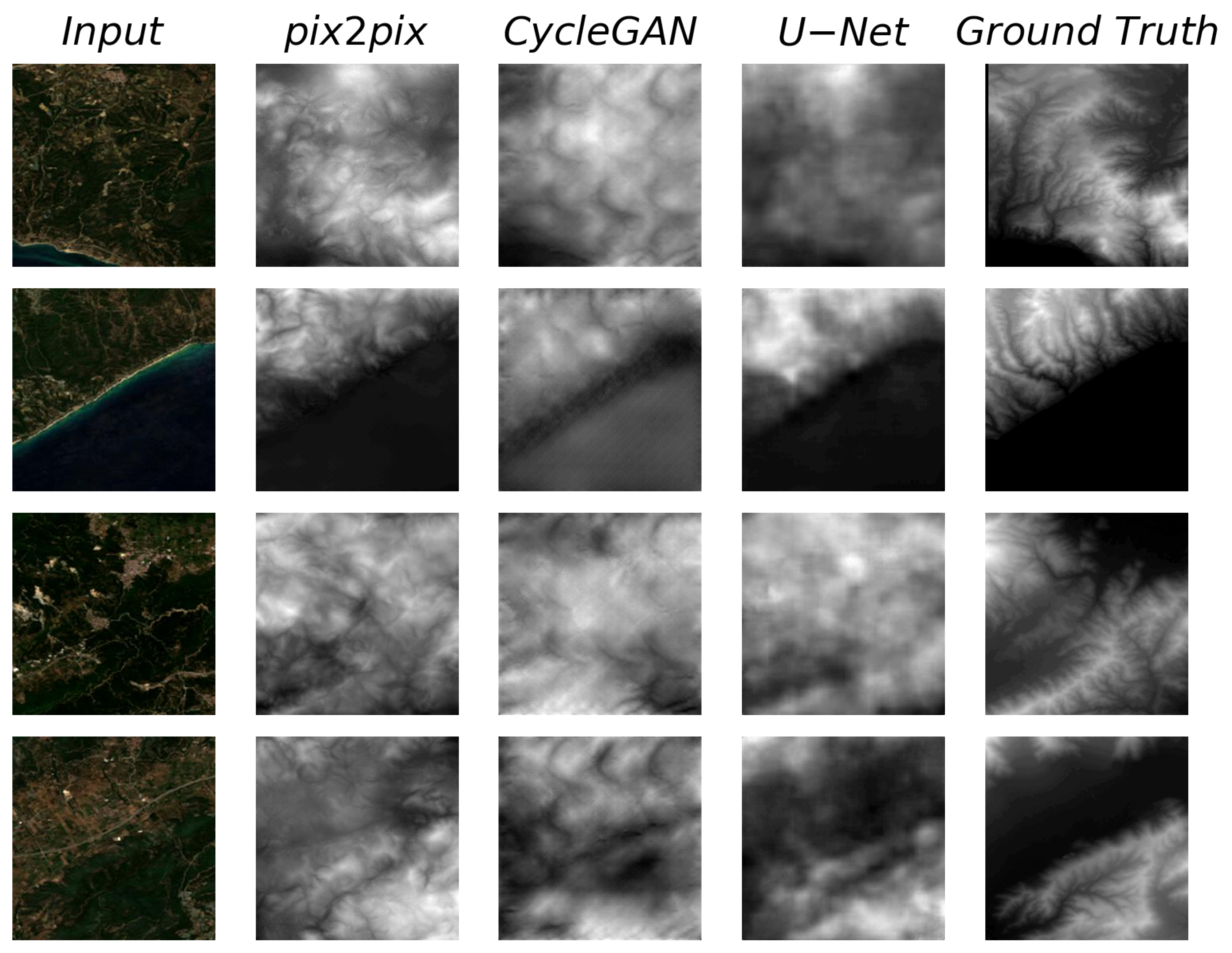
Qualitative comparison of performance on the test set for pix2pix [55], CycleGAN [57], and U-net [45]. To make the comparison as fair as possible, we present results after equal amounts of training time. Therefore, the ratio of epochs is roughly 1 : 0.6 : 0.17 for the U-net, pix2pix and CycleGAN respectively. It is evident that pix2pix achieves the most elaborate and accurate results compared to the competition. Note that the input satellite images were selected based on the complexity of the ground truth DEMs and not based on the performance of the models and that no data augmentation (Section 2.8) was used for this comparison. Therefore, these results are not indicative of an optimal state of the models and we have to extrapolate on the performance on bigger datasets. Representative results for pix2pix can be found in Figure 8. A quantitative comparison is presented in Table 3.
Figure 14.
Qualitative comparison of performance on the test set for pix2pix [55], CycleGAN [57], and U-net [45]. To make the comparison as fair as possible, we present results after equal amounts of training time. Therefore, the ratio of epochs is roughly 1 : 0.6 : 0.17 for the U-net, pix2pix and CycleGAN respectively. It is evident that pix2pix achieves the most elaborate and accurate results compared to the competition. Note that the input satellite images were selected based on the complexity of the ground truth DEMs and not based on the performance of the models and that no data augmentation (Section 2.8) was used for this comparison. Therefore, these results are not indicative of an optimal state of the models and we have to extrapolate on the performance on bigger datasets. Representative results for pix2pix can be found in Figure 8. A quantitative comparison is presented in Table 3.


Table 1.
Details of the bands used in the Multispectral extension of the satellite-imagery dataset.
| Band Name | Description | Wavelength |
|---|---|---|
| B2 | Blue | nm (S2A)/ nm (S2B) |
| B3 | Green | nm (S2A)/ nm (S2B) |
| B4 | Red | nm (S2A)/665 nm (S2B) |
| B5 | Red Edge 1 | nm (S2A)/ nm (S2B) |
| B6 | Red Edge 2 | nm (S2A)/ nm (S2B) |
| B7 | Red Edge 3 | nm (S2A)/ nm (S2B) |
| B8 | NIR | nm (S2A)/833 nm (S2B) |
| B8A | Red Edge 4 | nm (S2A)/864 nm (S2B) |
| B11 | SWIR 1 | nm (S2A)/ nm (S2B) |
Table 2.
Absolute (in meters) error and percentage error with respect to the total range of no regularization (W/O), L2 regularization () and diminished capacity (Less parameters) on test error of the satellite-imagery dataset. Note that the global maximum for the dataset was 3016 and the minimum . While at first glance the errors appear large, one has to take into consideration the fact that no ground truth elevation is provided to the model at inference time, so a added constant that does not alter the relative configuration of the terrain can result in large errors. Therefore, the model is successful in managing to restrict its output to a small range around the actual elevation while also preserving the relative geometry of the terrain. Note that we reduce the number of epochs per run to make several configurations and several runs for each possible.
| Method | Absolute Error (meters) | Percentage Error |
|---|---|---|
| W/O | % | |
| Less parameters | % | |
| % | ||
| % | ||
| % |
Table 3.
Absolute (in meters) error and percentage error with respect to the total range of the pix2pix, CycleGAN and U-net. To make the comparison as fair as possible, we present results after equal amounts of training time. Therefore, the ratio of epochs is roughly 1:0.6:0.17 for the U-net, pix2pix and CycleGAN respectively. Notice that producing sharp results (Figure 14) does not correlate well with quantitative performance, presumably due to overfitting. For the U-net especially, this can be attributed to the diminished capacity resulting from its simpler architecture, as we demonstrate in Section 3.2.
| Architecture | Absolute Error (meters) | Percentage Error |
|---|---|---|
| pix2pix | % | |
| CycleGAN | % | |
| U-net | % |
© 2020 by the authors. Licensee MDPI, Basel, Switzerland. This article is an open access article distributed under the terms and conditions of the Creative Commons Attribution (CC BY) license (http://creativecommons.org/licenses/by/4.0/).
Share and Cite
MDPI and ACS Style
Panagiotou, E.; Chochlakis, G.; Grammatikopoulos, L.; Charou, E. Generating Elevation Surface from a Single RGB Remotely Sensed Image Using Deep Learning. Remote Sens. 2020, 12, 2002. https://0-doi-org.brum.beds.ac.uk/10.3390/rs12122002
AMA Style
Panagiotou E, Chochlakis G, Grammatikopoulos L, Charou E. Generating Elevation Surface from a Single RGB Remotely Sensed Image Using Deep Learning. Remote Sensing. 2020; 12(12):2002. https://0-doi-org.brum.beds.ac.uk/10.3390/rs12122002
Chicago/Turabian StylePanagiotou, Emmanouil, Georgios Chochlakis, Lazaros Grammatikopoulos, and Eleni Charou. 2020. "Generating Elevation Surface from a Single RGB Remotely Sensed Image Using Deep Learning" Remote Sensing 12, no. 12: 2002. https://0-doi-org.brum.beds.ac.uk/10.3390/rs12122002
Note that from the first issue of 2016, this journal uses article numbers instead of page numbers. See further details here.