Persistent Vegetation Greening and Browning Trends Related to Natural and Human Activities in the Mount Elgon Ecosystem

Abstract

Many developing nations are facing severe food insecurity partly because of their dependence on rainfed agriculture. Climate variability threatens agriculture-based community livelihoods. With booming population growth, agricultural land expands, and natural resource extraction increases, leading to changes in land use and land cover characterized by persistent vegetation greening and browning. This can modify local climate variability due to changing land–atmosphere interactions. Yet, for landscapes with significant interannual variability, such as the Mount Elgon ecosystem in Kenya and Uganda, characterizing these changes is a difficult task and more robust methods have been recommended. The current study combined trend (Mann–Kendall and Sen’s slope) and breakpoint (bfast) analysis methods to comprehensively examine recent vegetation greening and browning in Mount Elgon at multiple time scales. The study used both Moderate Resolution Imaging Spectroradiometer (MODIS) Normalized Difference Vegetation Index (NDVI) and Climate Hazards group Infrared Precipitation with Stations (CHIRPS) data and attempted to disentangle nature- versus human-driven vegetation greening and browning. Inferences from a 2019 field study were valuable in explaining some of the observed patterns. The results indicate that Mount Elgon vegetation is highly variable with both greening and browning observable at all time scales. Mann–Kendall and Sen’s slope revealed major changes (including deforestation and reforestation), while bfast detected most of the subtle vegetation changes (such as vegetation degradation), especially in the savanna and grasslands in the northeastern parts of Mount Elgon. Precipitation in the area had significantly changed (increased) in the post-2000 era than before, particularly in 2006–2010, thus influencing greening and browning during this period. The greenness–precipitation relationship was weak in other periods. The integration of Mann–Kendall and bfast proved useful in comprehensively characterizing vegetation greenness. Such a comprehensive description of Mount Elgon vegetation dynamics is an important first step to instigate policy changes for simultaneously conserving the environment and improving livelihoods that are dependent on it.

1. Introduction

Vegetation plays very important roles in ecosystem processes, including the mitigation of climate change effects [1] and the regulation of land surface temperatures, carbon and energy cycles [2,3,4]. At the same time, significant changes in terrestrial vegetation have been reported in the recent past [5,6]. Previous studies have concluded that these changes are driven by (1) slowly-changing natural processes, such as regional climate change (e.g., changes in temperature, precipitation, etc.), nitrogen disposition and increasing atmospheric CO₂ concentrations [7], and (2) more rapid anthropogenic activities, including land-use and land-cover (LULC) change (e.g., deforestation [8,9], overcultivation and overgrazing [8], afforestation, expanding green areas in cities [1] among others). These processes do not operate in isolation [7] but rather interact at multiple scales, with global-scale drivers interacting with processes at the regional and local scales [10], thus making vegetation change dynamics a complex phenomenon to examine. Understanding vegetation dynamics has attracted substantial attention in the past years, specifically in the wake of climate change and variability [11]. As such, knowledge of vegetation response to climate change is critically important in the effort to maintain the supported processes as well as the human livelihoods derived from them [12]. Such an analysis has been difficult in the past, due in part to limited access to consistent data both in space and time. However, with recent developments in Earth observation (EO) technologies, spatio-temporally contiguous remote sensing (RS) data have been collected, making it possible to investigate vegetation dynamics accurately and comprehensively in terms of other environmental processes, at multiple scales.

The Normalized Difference Vegetation Index (NDVI), which is the normalized sum of the difference in reflectance between near infrared and red bands, has extensively been used [5,10,13] as an indicator of photosynthetic activity and vegetation amount [14]. Previous studies used this vegetation index (VI) to characterize vegetation processes such as productivity decline [6], phenology [15,16] and greening and browning [1,5,10,12,17,18]. Variability in NDVI generally follows patterns of climatic conditions, mainly precipitation [11,19,20,21,22]. The NDVI–precipitation relationship is largely a strong positive one, particularly in locations where total annual precipitation is less than 1000 mm [19,22]. This relationship is further compounded in space and time by site-specific factors such as existing LULC, vegetation structure and composition [22], topography [10] and soil type [23]. As a result, vegetation greenness response to climate has shown significant spatial and temporal variability. For instance, contrasting natures and strengths of the NDVI–precipitation relationship have been reported: a strong linear relationship in the Sahel [19] and a log-linear one in East Africa [22]. In other studies, seasonal precipitation with different lag times was found to correlate strongly with NDVI [13,22]. This complexity implies that (i) results from a specific regional analysis are not transferable to another region; (ii) any slight spatial and/or temporal misspecification may lead to misleading results about vegetation greenness–precipitation relationships and patterns; and (iii) understanding vegetation change requires multiple images (time series, TS) as opposed to the extensively used traditional classification and change detection methods.

East Africa depends heavily on rainfed agriculture, which puts food security and rural livelihoods at risk [24]. The importance of land in this region cannot be overemphasized [24], yet land holdings are small and steadily declining [24,25]. At the same time, populations have been increasing thus necessitating expansion of food production while also navigating the effects of climate change in the area. Over recent decades, therefore, East Africa has witnessed significant landscape transformation due to both human and natural drivers [6,26]. Generally, natural vegetation has been converted to farmlands, grazing lands and human settlements [25]. This LULC transformation has been reported in the Mount Elgon ecosystem (MEE), a major water catchment tower supplying water to three major lakes in East Africa (Lake Turkana, Kenya, Lake Kyoga, Uganda and Lake Victoria, Kenya, Uganda and Tanzania [27]). The MEE is dominated by croplands in most locations, mixed vegetation (primarily savanna, grasslands, and shrubs) in the northern portion and the Afromontane forest (Figure 1). The high population growth and densities in the area have translated into need for more land [28]. Coupled with political interference and corruption among park and reserve staff, the need for more land has resulted in forest encroachment and deforestation as ecologically fragile land is cleared for agriculture and settlement [28,29,30,31,32]. The changes in LULC have, in part, altered the functioning of the ecosystem [29] and, as a result, the mountain area has experienced more frequent landslides, prolonged droughts, and flooding [30,31]. Evidence of a changing climate has been reported [33] and this may result in increased frequency of these events. As such, the livelihoods of at least 2 million people [27,31] are threatened. Despite this, the complex MEE landscape is currently understudied. A key study of LULC change was conducted by Petersson, Vedeld, and Sassen [27] and employed institutional theory in analyzing processes that led to deforestation within protected areas (PAs) in the transboundary MEE. It was found that, especially on the Kenyan side, it was challenging to correctly quantify LULC change due to the overlap between bamboo, plantation and Shamba system farms. Other studies have been conducted on relatively smaller spatial scales, mostly on the Ugandan side. Such studies have focused on the effect of LULC change on landslide occurrence [28], soil organic carbon, food security and climate change vulnerability [34], carbon stocks and climate variability [35] among others. However, some of the studies have reported contradictory results especially about the magnitude of LULC change within the agricultural land-use class. This may be due to the complex LULC orientation, which leads to persistent greening and browning in the MEE, thus making it difficult to correctly characterize vegetation dynamics especially using traditional classification and change detection methods. More robust methods are therefore needed, and TS analysis has been applied to comprehensively examine spatio-temporal landscape changes, particularly for constantly variable landscapes like the MEE.

TS analysis of RS data has been used to characterize environmental phenomena by describing both trends and discrete change events [37]. In recent years, application of TS methods has increased and this has been driven by improved access to RS imagery (for instance, due to opening up of the Landsat archive in 2008 [38]), improvements in the integration of RS and GIS (Geographic Information Systems) and general advancements in computing power [39]. As such, analysis of LULC change, including vegetation greening and browning, has significantly evolved from the traditional bitemporal image analysis to using multiple and continuous observations. Common methods for TS analysis include Fourier analysis [40,41], principal components analysis, [42,43] and the Mann–Kendall statistic [44]. The Mann–Kendall statistic has been used to identify the presence and nature of monotonic trends in vegetation time series [5,10,45]. It is a non-parametric statistic; thus, data does not have to conform to any specific distribution [46]. Besides, Mann–Kendall compares relative magnitudes of sample data instead of raw data values and therefore missing values are allowed in the analysis. The Mann–Kendall analysis is often followed by the Sen’s slope estimator [47], which quantifies the strength of the monotonic trends [12,45]. The Sen’s slope estimator calculates the median of the set of slopes generated from Mann–Kendall [47]. Mann–Kendall and Sen’s slope have been found to be more robust for TS with outlying values as compared to parametric statistics like ordinary least squares [12]. These two statistics identify and quantify any overall trends in a time series and are therefore well suited for examining vegetation greening and browning. Previous studies have successfully used these methods in assessing the consistency of greening and browning patterns across spatio-temporal scales in northern India [12] and assessing variability in greening and browning patterns caused by use of different RS imagery in the boreal forest of central Canada [48]. However, the assumption that the vegetation trend preserves its change rate throughout the period of study means that some greening and browning changes are masked [5]. For instance, later greening in a consistently browning vegetation may not be detected using Mann–Kendall and Sen’s slope. To counter this issue, more TS decomposition methods have been proposed, including Breaks for Additive Season and Trend, bfast [16]. Using bfast, even subtle changes in vegetation can be monitored. This algorithm has successfully been used in delineating anthropogenic, fire and elephant damage within forest ecosystems in Kenya [49]. Complementing Mann–Kendall and Sen’s slope with bfast can therefore be valuable in examining vegetation greening and browning trends, especially in a dynamic environment like the MEE. In such an analysis, the latter can be used to characterize changes detected by the former. Vegetation trends can then be characterized in more detail and this can be the basis for understanding effects of climate on terrestrial ecosystems [5] and the development of ultimate strategies for the sustainable management of ecosystems [10].

The goal of this study was to characterize comprehensively, over multiple time scales, recent patterns and trends in MEE vegetation greening and browning. Here, the main objectives were; (1) to assess and quantify the nature and magnitude of change in MEE greenness for the period 2001–2018; and (2) to characterize trends and variability in MEE precipitation as a way to disentangle nature- versus human-driven vegetation greening and browning. It is hypothesized that (1) changes in climate have forced local communities in the MEE to expand croplands at the expense of the natural vegetation thus leading to deforestation and degradation; and (2) the high variability exhibited in the MEE landscape requires integration of both general (such as Mann–Kendall and Sen’s slope) and sequential (such as bfast) TS analysis methods to be fully characterized. To achieve these goals, the study analyzed spatio-temporal trends and patterns in Moderate Resolution Imaging Spectroradiometer (MODIS) NDVI (2001–2018) and Climate Hazards group Infrared Precipitation with Stations (CHIRPS) precipitation (1986–2018) at multiple temporal scales (dekadal (10-day), 16-day, seasonal), using an integration of Mann–Kendall, Sen’s slope and bfast algorithms. The study also incorporates inferences from a field study conducted in the MEE in 2019 to explain some of the vegetation change dynamics in the area. This analysis thus produces a more comprehensive characterization of vegetation dynamics in the MEE, which would not be possible using traditional classification and change detection methods. Results would help fill in some of the existing gaps in literature about nature and magnitude of LULC change and the stability of LULC in the MEE. Such a comprehensive description of MEE vegetation dynamics is an important first step to initiate dialogue aimed to instigate policy changes for simultaneously conserving the environment and improving livelihoods dependent on it.

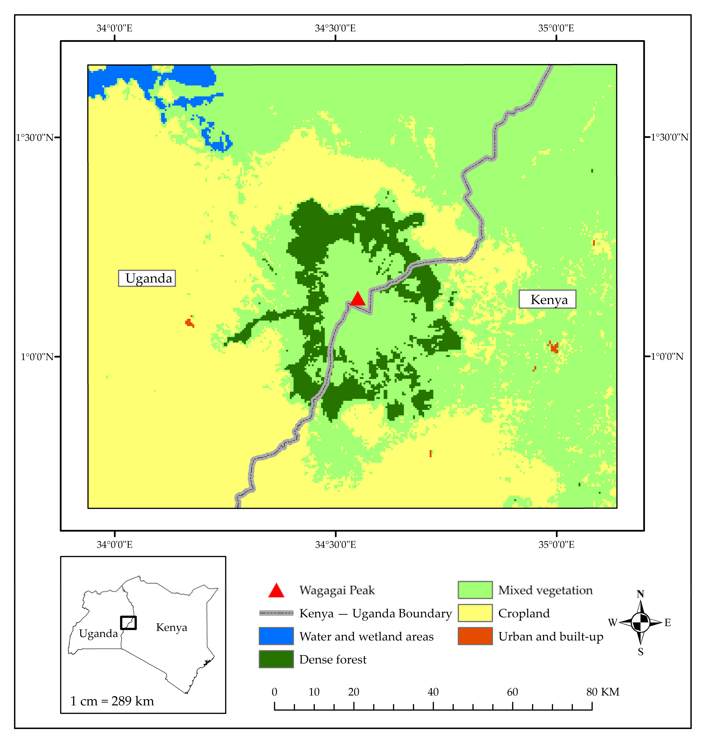
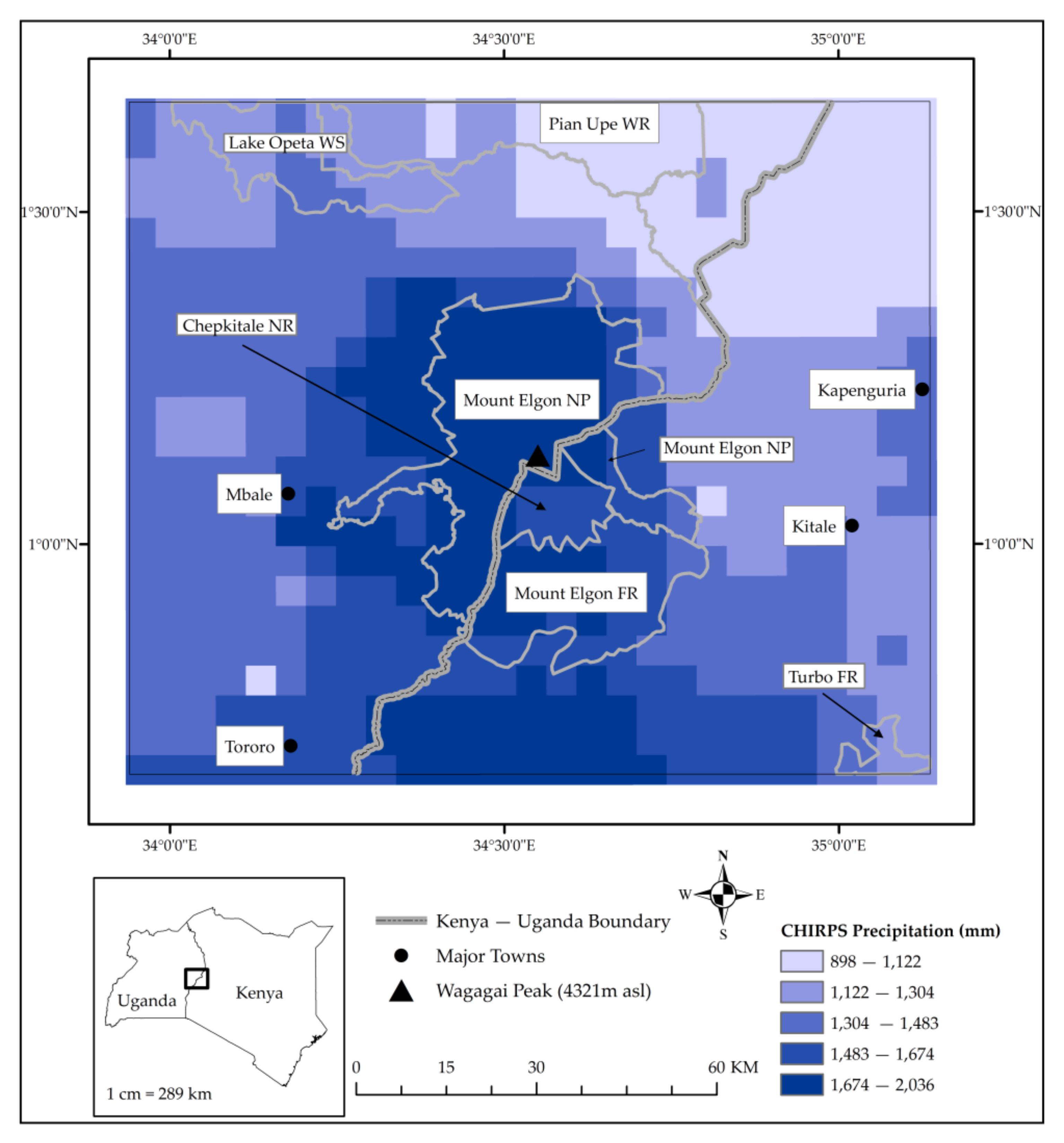
2. Study Area Description

The MEE is located in western Kenya and eastern Uganda (Figure 1 and Figure 2). The studied area covers approximately 15,000 km² and extends from 1°37′42.82″ N, 33°55′45.07″ E and 0°42′15.76″ N, 35°14′18.84″ E. Mount Elgon is a solitary volcano and is among the oldest in East Africa [28,32]. The highest point, Wagagai Peak, is 4321 m [28,50] and is found on the Ugandan side. This area rises from a plateau that lies 1850–2000 m in the east and 1050–1350 m to the west with a caldera that extends 8 km wide [50]. Vegetation in this area is zoned by altitude and mountain forest, farmland and Afro-Alpine heath and moorland are the common land covers [27]. Declared a protected area in 1968 and 1992 in Kenya and Uganda, respectively [31,51], Mount Elgon Forest, a montane rainforest [52], is home to many important indigenous tree species [27].

The MEE receives rainfall in a bimodal pattern (two rainy seasons) and, according to Mugagga, Kakembo and Buyinza [28], most of the rainfall is received between April and October on the Ugandan side (with mean annual amounts ranging from 1500 to 2000 mm). The Kenyan side receives long rains between March and June and short rains between September and November—average annual rainfall ranging from 1400 to 1800 mm [54,55]. There is minimal temperature variation for the area—an average minimum of 15°C and a maximum of 23°C on the Ugandan side [28] and 14 and 24°C on the Kenyan side [55]. However, temperatures and precipitation have a strong variation with changes in altitude [27].

3. Materials and Methods

The present study integrated Mann–Kendall, Sen’s slope and bfast in the analysis of NDVI and precipitation trends to characterize recent greening and browning patterns and trends within the MEE.

3.1. Data and Sources

This study utilized the following datasets (

Table 1. Description of original datasets used in the study.

Dataset	Spatial Resolution	Temporal Resolution	Duration	Source
MODIS MOD13Q1.V6	250 m	16-day	2001–2018	https://lpdaacsvc.cr.usgs.gov/appeears/
CHIRPS	5 km	5-day	1986–2018	https://earthengine.google.com/

) in the analysis of greening and browning trends in the MEE.

3.1.1. MODIS NDVI and CHIRPS Precipitation

This study used MODIS NDVI data in the TS analysis of spatio-temporal changes in MEE vegetation greenness signal. The 16-day NDVI composite MOD13Q1.V6 [56] with a 250-meter spatial resolution was obtained through AppEEARS (https://lpdaacsvc.cr.usgs.gov/appeears/) [57]. Data for the period 2001–2018 were used. While Landsat data [58] have a better spatial resolution and historical coverage, and are therefore better suited for this study, they were limited by the many data gaps in the TS over the MEE due to persistent cloud cover and Landsat’s long (16-day) revisit time. As such, MODIS NDVI, which has previously been used successfully in similar studies in East Africa [6,22,59], was used in this study. This study also used CHIRPS precipitation data [53]. These data have a spatial resolution of 5 km and provide global daily and pentad records from 1981 to present. For this study, these data for the period 1986–2018 were obtained and preprocessed within Google Earth Engine (GEE) [60]. It is worth noting here that there were no observation data to assess the accuracy of the CHIRPS dataset over the MEE. However, this dataset has been used extensively in similar studies [12,61,62]. Moreover, this dataset was recently validated [63] and the results showed that the CHIRPS data are reasonably accurate in estimating rainfall over east and South Africa.

NDVI preprocessing involved quality assessment using the associated VI quality files. Pixels with low quality, high aerosol content, cloud cover and possible shadows were excluded during this exercise. NDVI and precipitation composites for specific time scales were then generated. First computed were mean NDVI TS during the wet season for the period 2001–2018. Here, imagery in April, May and June was used. The TS of mean NDVI for each 16-day period during the season were also created. As a result, there were generally two TS for each month and were labeled h1 and h2 for TS created from NDVI composites recorded roughly in the first and second half of the month, respectively. For precipitation, the TS of total amount over the wet season were computed for different periods; 1986–2018 (33 years); 1986–1996 (first 11 years); 1997–2007 (median 11 years); 2008–2018 (last 11 years); 1986–2005 (first 20 years); 1999–2018 (last 20 years); and 2001–2018 (18 years, similar to the NDVI TS length). While the present study was aimed at characterizing changes in vegetation greenness from 2001 to 2018, analysis of longer precipitation TS was necessary to understand any longer-term precipitation patterns in the MEE that may influence the vegetation patterns. TS were also generated of total precipitation amounts for each dekad over the wet season. In this analysis, these dekads for the month of April were labelled April d1 (for dates 1–10), April d2 (for dates 11–20) and April d3 (for the rest of the month). The same nomenclature was used for dekad TS in May and June. These were used to assess nature and strength of relationship between vegetation greenness and precipitation variability over a shorter time scale, in which case results from dekad precipitation TS were compared to results from 16-day NDVI. The 16-day NDVI composites were used here due to unavailability of data to compute dekad NDVI composites. Finally, monthly precipitation composites were generated for the period 1986–2018, for use in analyzing breakpoints in MEE precipitation.

3.1.2. Field-Collected Data

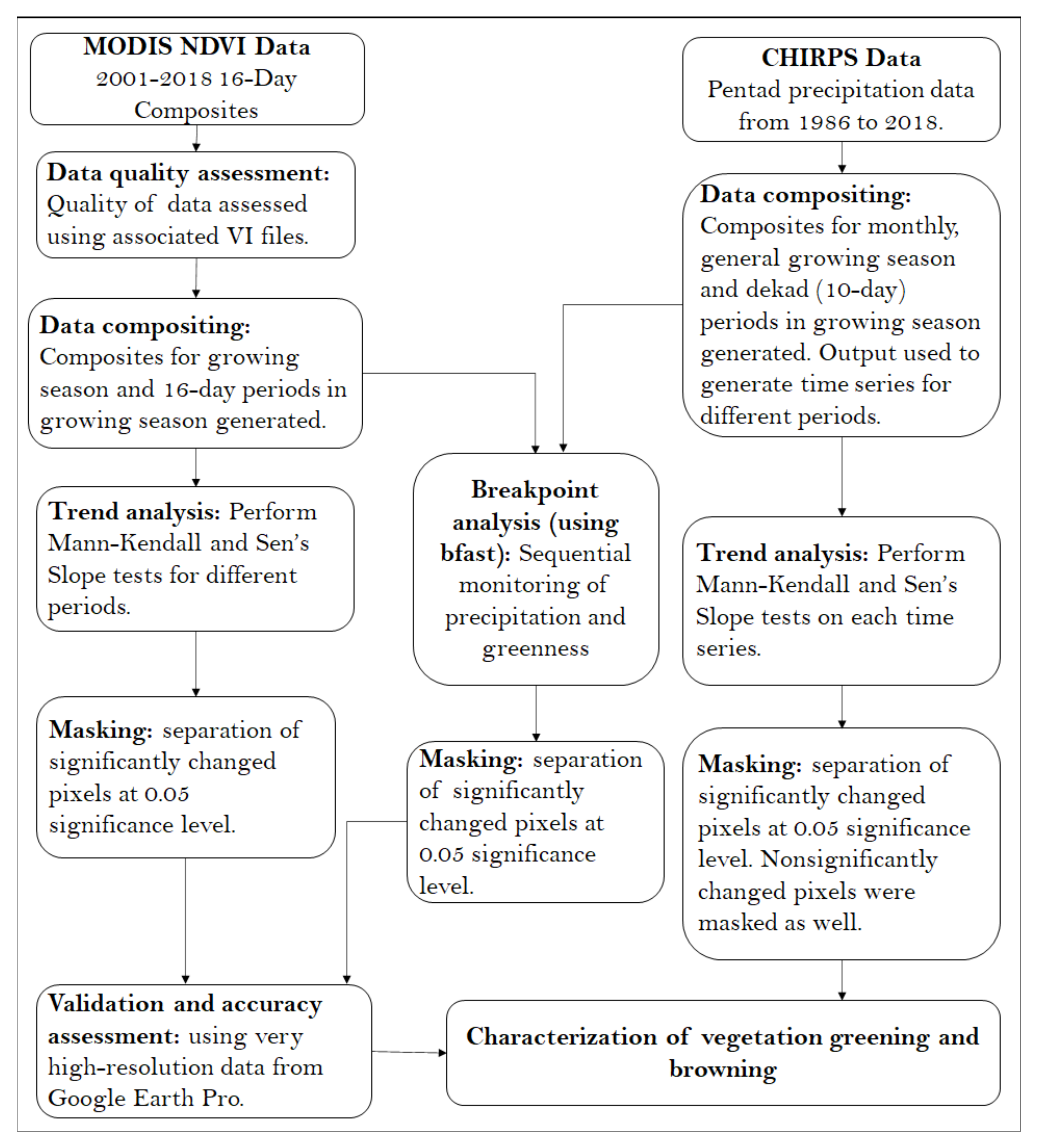
Environmental data from local communities and government officers within the MEE were collected using semi-structured interviews and direct observation in July–September 2019 (IRB Number: STUDY00002404). Most of the interviewees were from significantly changing landscapes (areas showing significant changes in vegetation greenness). The participants in this study were interviewed about perceptions of climate change and land-use change, and historical patterns of agriculture and land-use change. Interviews were conducted and written responses recorded using Qualtrics software [64]. The fusion of such qualitative data with quantitative RS data is important because indigenous and historical accounts of LULC change in such a constantly variable landscape can be used to fill in gaps that may not be fully explained using RS and GIS alone.

3.2. Methods

This section describes the methods and analyses performed on NDVI and precipitation TS to identify areas and characterize patterns of vegetation greening and browning within the MEE. These two analyses were performed in R [65] and trends were assessed at the 95% significance level. After analysis of monotonic trends in greenness and precipitation, it was necessary to perform breakpoint analysis on these time series, to detect any significant breaks within the data. These two types of analyses are described in more detail below. Figure 3 highlights major methods used in this study.

3.2.1. TS Analysis: Mann–Kendall and Sen’s Slope

To analyze initial spatiotemporal changes in vegetation greening and browning trends in the MEE, the current study borrowed from methodologies presented by Landmann and Dubovyk [6]. However, since NDVI TS often do not meet assumptions for parametric analysis [48], the current study used the nonparametric Mann–Kendall test rather than linear regression. To calculate the Mann–Kendall test statistic, data values are evaluated as an ordered TS [46] and each value is then compared to all subsequent values [46,66]. The Mann–Kendall S statistic is initially assumed to be 0 and a value of 1 is added to (subtracted from) the test statistic if the value of an observation is higher (lower) than that of the previous observation [46,66]. There is no change to the statistic if the values are equal. Equation (1) below shows the Mann–Kendall test equation. High positive and low negative values of S, respectively, indicate increasing and decreasing trends, but the strength of the trend is statistically quantified by computing probability associated with S and the size of the data sample [46].

$$\mathrm{S}={\displaystyle \sum }_{k=1}^{n-1}{\displaystyle \sum }_{j=k+1}^{n}sign\left(x_j-x_k\right)$$

(1)

where   $sign\left(x_j-x_k\right)$ = 1   if $x_j-x_k > 0$

           = 0   if $x_j-x_k = 0$

           = −1   if $x_j-x_k < 0$ Source: Khambhammettu [46]

The magnitude of the trends was quantified using Sen’s slope estimator [47]. These algorithms were used in this study first to characterize and quantify any general patterns in MEE greenness during the growing season (April, May, and June). The analysis then investigated more subtle changes in vegetation greenness over shorter (16-day) periods during the growing season. From these, areas of increasing (decreasing) greenness were mapped as areas of vegetation greening (browning).

To disentangle changes due to human and natural forcings, monotonic trends were assessed in the precipitation TS and magnitude of the trends quantified. The analysis was performed on precipitation series at different temporal scales—based on the length of the time series (including 33-, 20-, 18- and 11-year periods) and TS resolution (including dekad totals, and general growing season totals). From these analyses, areas with significant positive (negative) precipitation trends were mapped as areas experiencing significant and consistent wetting (drying) over the analysis period. A cross examination of results from greenness and precipitation trend analysis was conducted to distinguish any human- from nature-driven vegetation greening and browning. Using available very-high-resolution imagery from Google Earth Pro [67], the nature of LULC conversion was ascertained. Besides, the statistics of LULC change (including greening, browning pixels) were calculated.

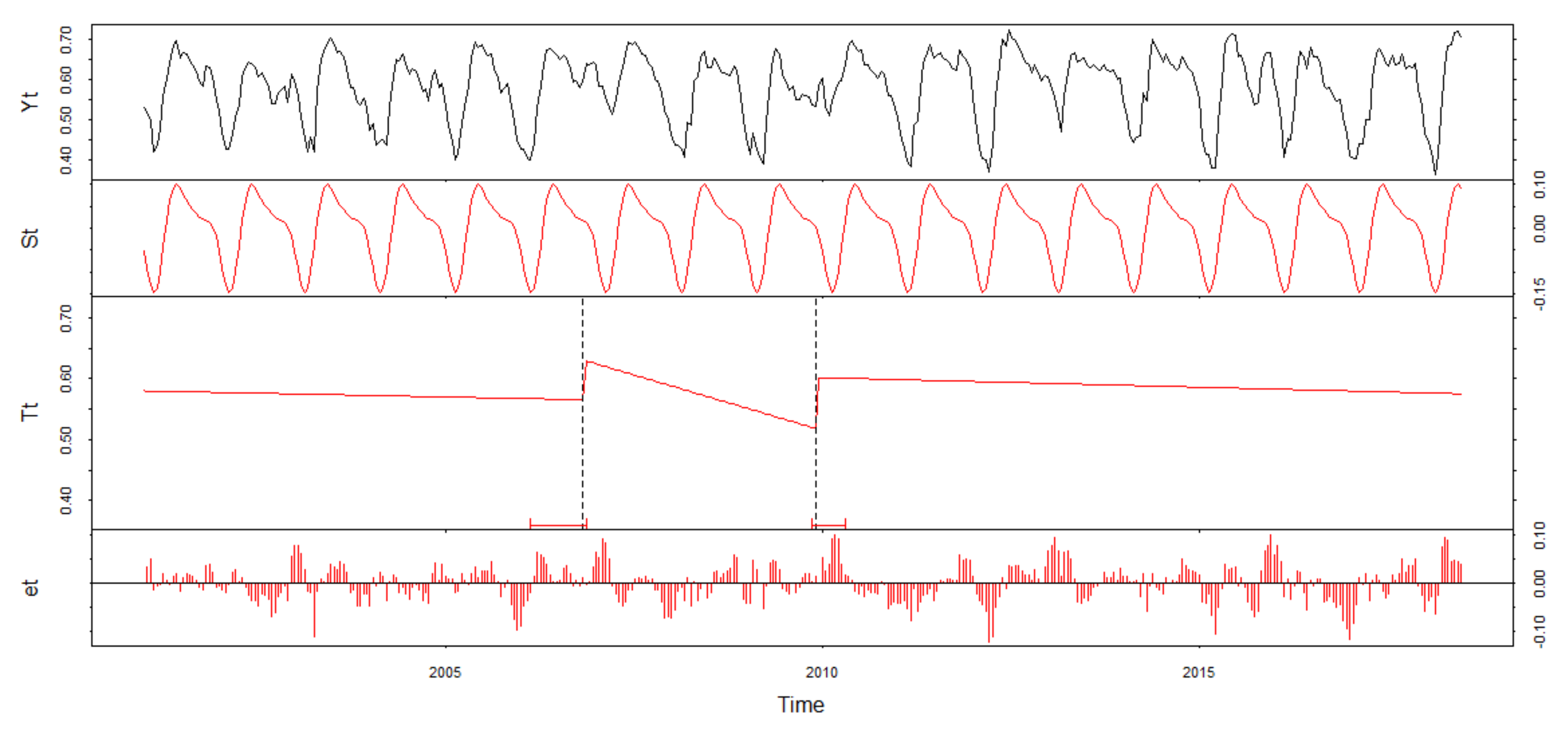
3.2.2. Breakpoint Analysis: bfast

To further understand any temporal patterns in MEE greenness and precipitation, the bfast algorithm was applied using the ‘bfastSpatial’ package (http://www.loicdutrieux.net/bfastSpatial/). There exists a predictable annual cycle of greening an browning in vegetation, and these coincide with the occurrence of rainy and dry seasons [49]. bfast, created by Verbesselt et al. [16] and Verbesselt and Zeileis [68], creates a best-fit seasonal regression model with a trend component for the time series [69]. This approach follows three main steps (i.) fitting a harmonic model based on a historical (‘stable’) period, (ii.) testing observations that follow the historical period for any structural breaks from the fitted model, and (iii.) calculating the magnitude of change which is the median residual between observed and expected values in the monitoring period [49,70]. While this approach has been applied on forested landscapes, the current study applied it to the whole of the MEE, whose LULC comprises forested, savanna, grassland, and cropland LULC (Figure 1). This was prompted by the unique LULC orientation in the MEE that makes it difficult to detect LULC changes via satellite image change detection analysis [27]. bfast breakpoint analysis can sequentially monitor vegetation change on a yearly basis, thus making it a suitable method for assessing changes in such LULC.

The models used in this part of the study were parameterized based primarily on the study by DeVries et al. [70]. First, the time series was divided into historical and monitoring periods. A minimum of two years for the historical period is recommended when using MODIS 16-day data [49,68]. In this study, therefore, the period 2001–2004 was used as the initial historical period and was assumed to be generally stable before the start of the monitoring period. First-, second- and third-order harmonic models were fit on the NDVI data, the results were assessed, and the first-order model was finally selected as the suitable instance to use. The single-order model has been used previously with the assumption that vegetation phenology generally follows a similar trend [70]:

$$y_t=\alpha +\gamma \sin (\frac{2\pi t}{f}+\delta )+{\epsilon }_t$$

(2)

where    yt   dependent variable

    t   independent variable

    f   temporal frequency

    α   model intercept

    γ   model amplitude

    δ   model phase

    ɛ_t   error term

As in the study by DeVries et al. [70], the trend component was excluded from the time series to reduce chances of yielding false breakpoints.

The change magnitude was calculated as the median of the residuals in the monitoring period. The median is thought of as a conservative measure, unlike the sum, that minimizes the chances of getting inflated magnitudes and therefore false breakpoints [70]. However, increasing the number of observations before and after a change event, by including long monitoring periods, yielded very high magnitudes and unrealistically numerous breakpoints. As such, this study elected to use sequential non-overlapping one-year-a-time monitoring periods. Here, the TS was trimmed to include the historical period plus one-year monitoring period. For monitoring the period from January to December 2005, for example, the TS for January 2001 to December 2005 was used, and the monitoring period was set to start in January 2005. This sequential monitoring approach is illustrated in DeVries et al. [70]. The approach is advantageous as it enables the assessment of subtle changes in vegetation within the MEE, especially alternating degradation and restoration that would go undetected using other methods. The default values for h, the minimal segment size between potentially detected breaks in the trend model given as a fraction relative to the sample size [49], were used in this study.

Breakpoint analysis was also performed on the monthly total precipitation TS. The analysis was performed on both 1986–2018 and 2001–2018 time series, to understand any longer-term patterns as well as recent changes in the precipitation. Here, the third-order harmonic model with the trend term was the best fit. While there was no direct application on record of bfast for precipitation breakpoint analysis, it is noted that the algorithm can be used for this purpose [71,72].

3.3. Validation of Results

A hybrid validation of analysis results was performed in this study. The collection of reference data borrowed from the methodology used previously by Landmann and Dubovyk [6]. The seasonal greening and browning map from Mann–Kendall and Sen’s slope analysis (Figure 4) was linked to very-high-resolution imagery in Google Earth Pro and both qualitative and quantitative accuracy assessment of the results was performed. Locations of greening, browning and no change were investigated by visually interpreting historical imagery in Google Earth Pro. The selection of these testing points was based on the minimum size of detectable change (at least 250 m, the size of a MODIS NDVI pixel) and the availability of sufficient imagery to interpret change. As such, only locations with very-high-resolution imagery in one of the three initial and final years (2001–2003, 2016–2018, respectively) were used. By visually assessing historical imagery spanning these periods, vegetation change, or lack thereof, could be observed. A total of 153 visually interpreted points (51 browned, 50 greened and 52 no change) were used. Greenness change in pixels at these locations was first recorded. The seasonal greening and browning map from Mann–Kendall and Sen’s slope analysis (Figure 4) was also reclassified into greened, browned and no change classes. The testing points were then compared to the reclassified raster and accuracy measures including overall, producer’s, and user’s accuracies were calculated. The final points were locations with pixels that indicated highly discernible change (like deforestation, reforestation etc.).

It was challenging to evaluate sequentially monitored vegetation change since it was not possible to gather testing points due to many temporal gaps in images in Google Earth Pro. In most instances, one can rarely find images for successive years, thus making it difficult to validate year-to-year change results. Since the bfast algorithm detects even subtle changes in vegetation greenness, changes could not be discerned with high confidence and therefore calculating accuracy assessment statistics would be misleading due to inconsistencies in testing data [73]. As such, these results were only visually and qualitatively assessed, and a general trend of change in the pixels was interpreted rather than year-to-year change. Evaluating such time series results has been found to be challenging previously [37,74]. In this study, inferences drawn from the field interviews were also qualitatively incorporated in this exercise to explain some of the trends detectable in both trend and breakpoint analyses.

4. Results

This study highlights and characterizes, using the Mann–Kendall, Sen’s slope and bfast algorithms, recent vegetation greening and browning trends and patterns in the MEE at multiple time scales. The results highlight portions of the MEE that experienced persistent and significant changes in vegetation greenness, as indicated by changing NDVI. The results from similar analyses of precipitation TS are also presented and, together, attempt to disentangle nature- from human-driven changes observed over the MEE landscape.

4.1. Trend Analysis Results

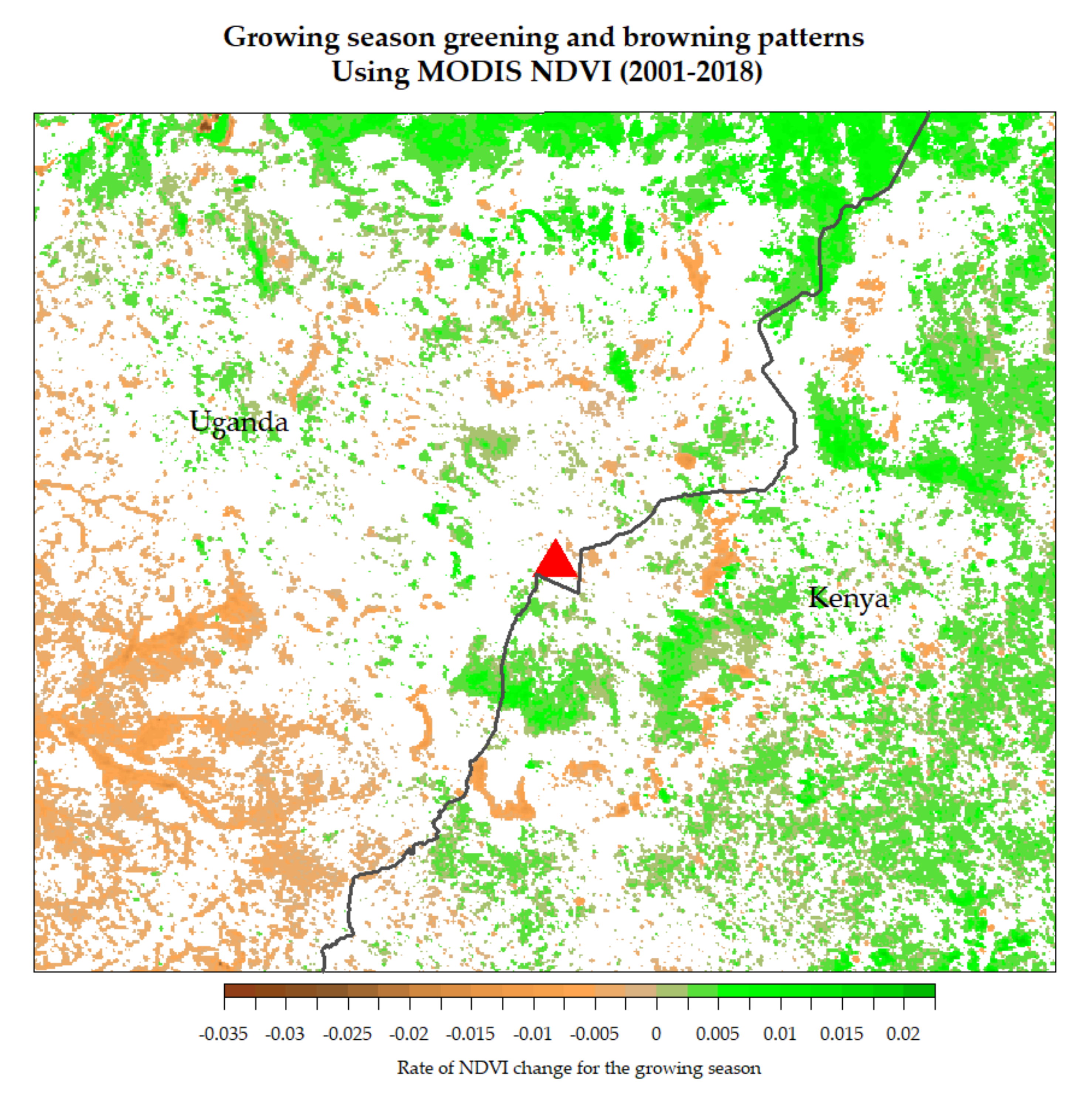
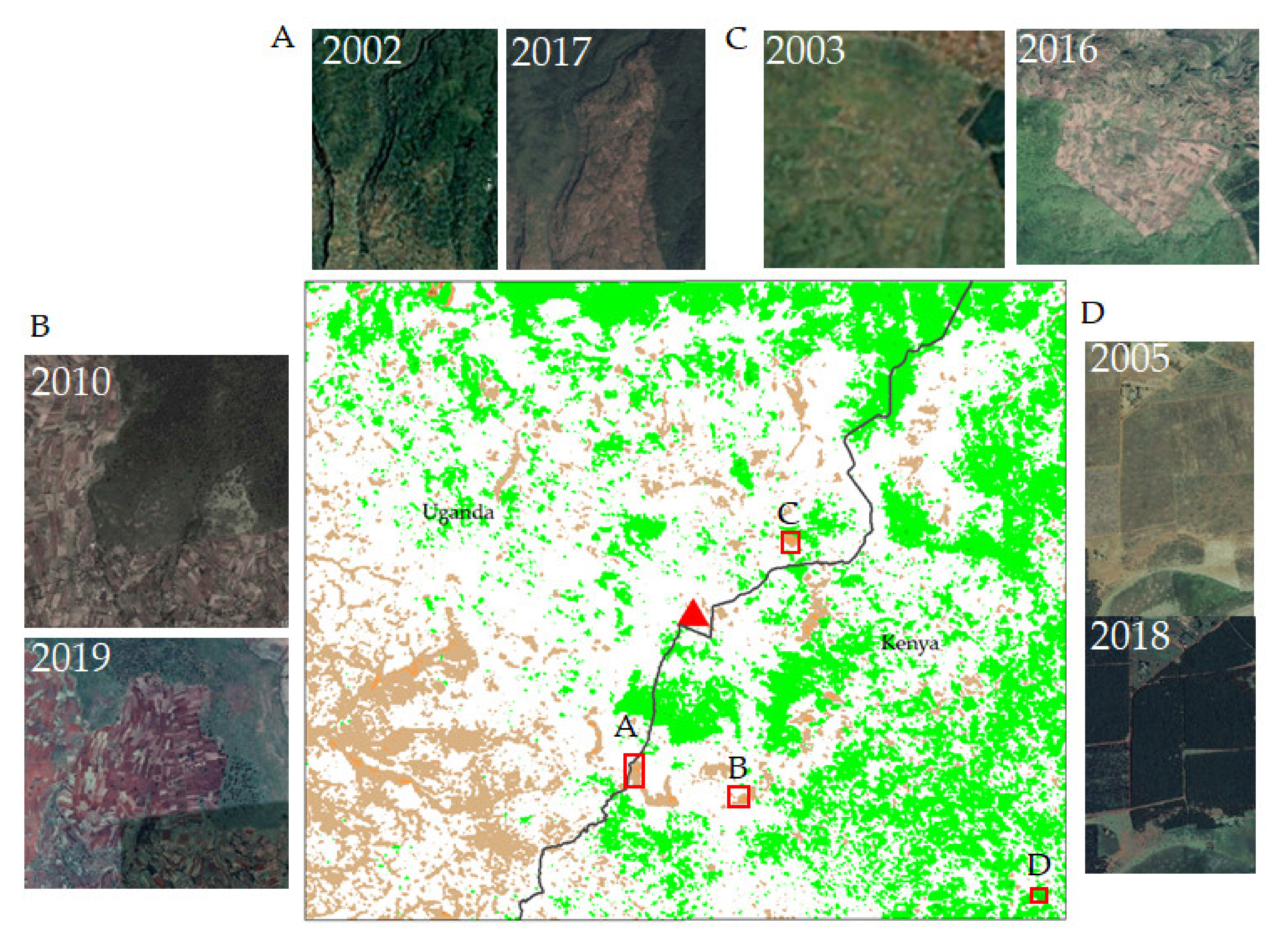
4.1.1. Persistent Vegetation Greening and Browning in the MEE

Greening (browning) was defined as any significant increase (decrease) in NDVI as shown by either Kendall τ (Mann–Kendall and Sen’s slope) or the magnitude of change (bfast). The results indicate various greening and browning patterns during the growing season (Figure 4) and near-half month (Figure 5) periods. During the growing season, greenness significantly increased in approximately 27% (3400 km²) of the study area. Here, NDVI increased at rates up to 0.025 per year. These locations were concentrated mostly within croplands, grasslands, and savanna (Figure 1). Significant browning was also evident, with NDVI in more than 1400 km² (about 11% of the total area) decreasing by up to 0.035 per year over the analysis period. These areas were mostly located in the southwestern part of the MEE in Uganda. This location includes the Namatala wetland, which has experienced intensive conversion to agriculture and settlement in the past years [75]. Browning was also evident in other locations around the Mount Elgon ecotone and elsewhere in the MEE. Based on our visual assessment, most of these corresponded to areas where deforestation occurred over the analysis period. No significant trends were found in the rest of the MEE (62%, 7800 km²).

Analysis of greening and browning trends in NDVI for every 16-day period in the months of April, May and June showed similar patterns; most browning occurred in the southwestern MEE and greening elsewhere. Most of the changed areas experienced greening and browning at rates of up to 0.03 and -0.04, respectively. The highest proportions of land where greening occurred was found in the month of May, especially the May h1 period, in which about 20% (2400 km²) of the MEE experienced significant greening (Figure 5). Greenness increased in more than 1600 km² (13%) of the study area during May h2. More greening was experienced in the June h2 and April h2 (9% of MEE greened during both periods). The greatest proportion of browned areas was observed in June h1, where about 600 km² (5%) of the MEE experienced vegetation greenness decline (Figure 5E). Most of the land within the MEE did not experience any significant change during these 16-day periods.

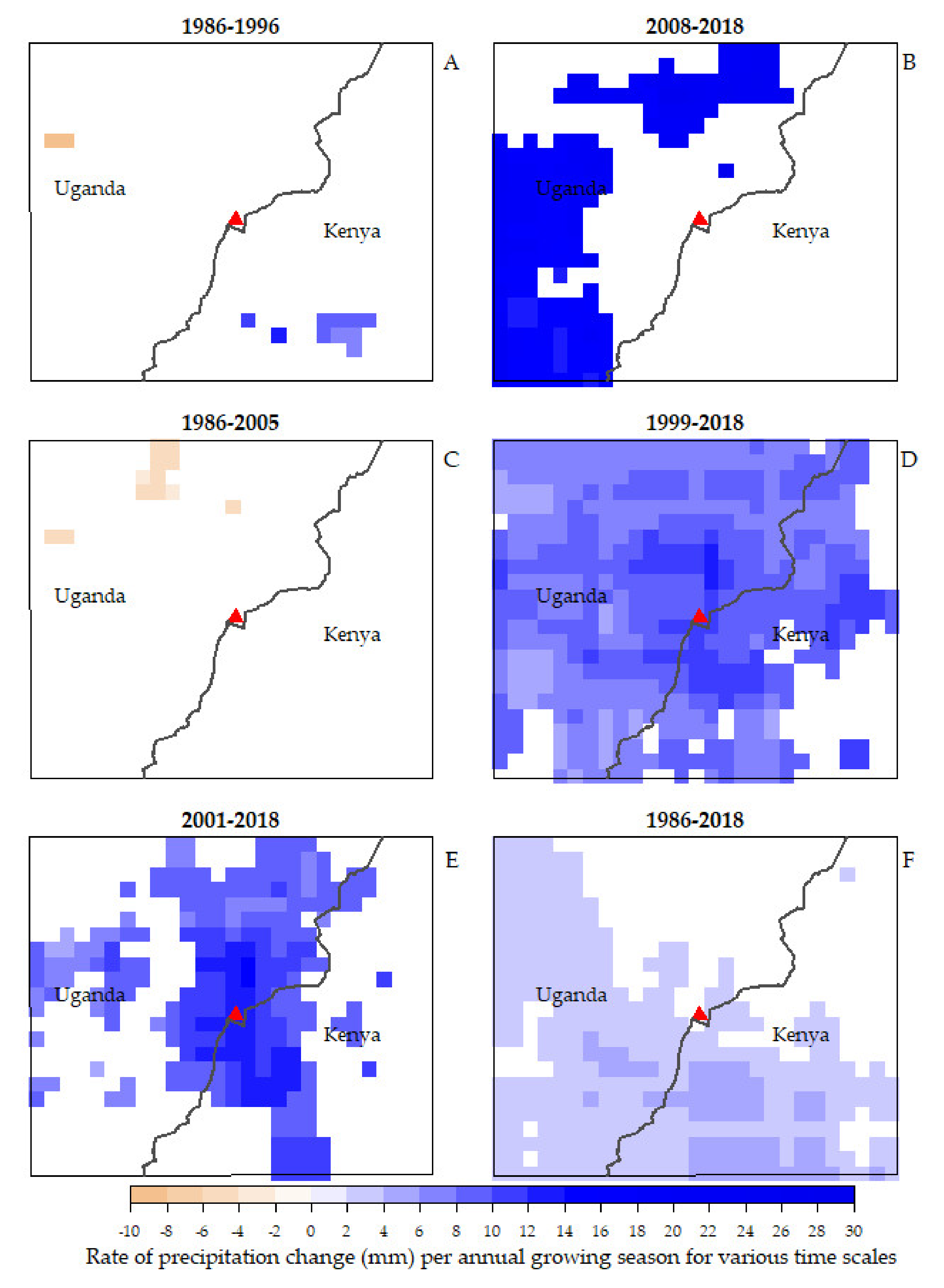
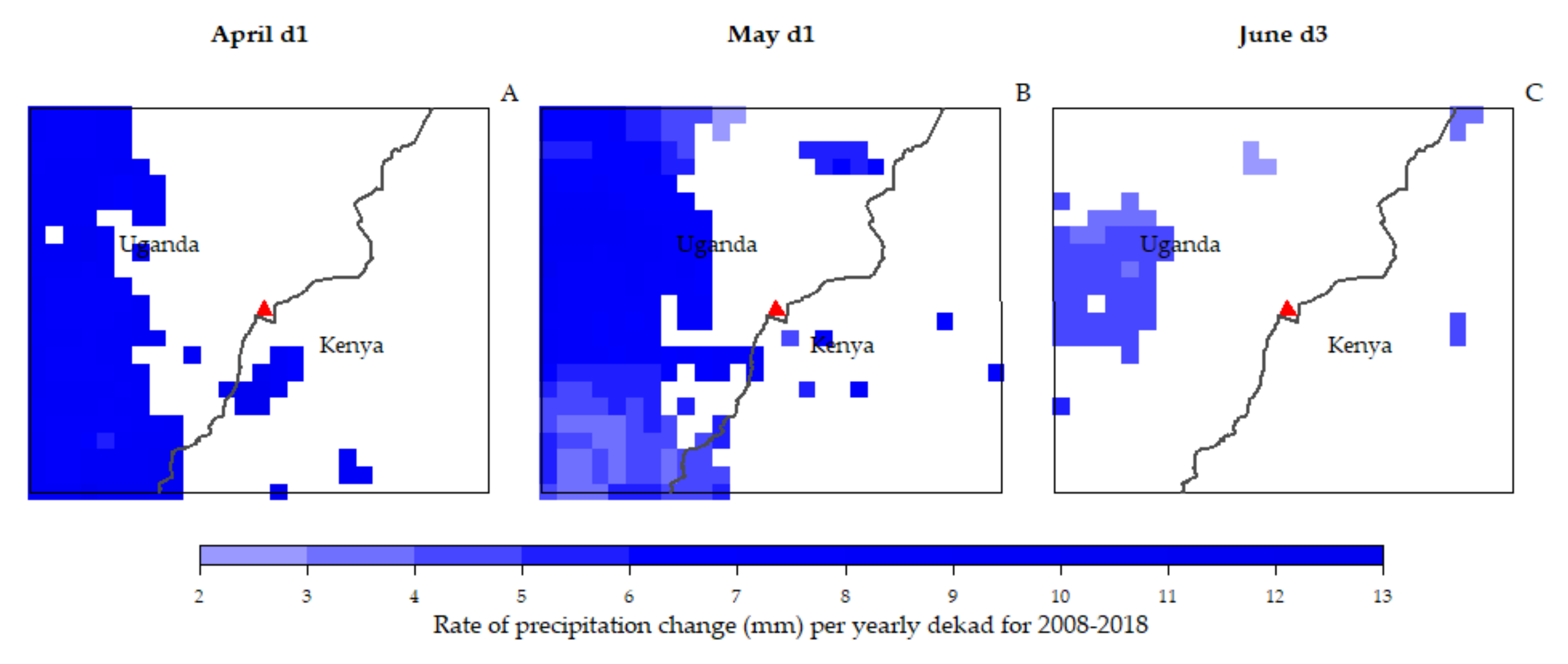
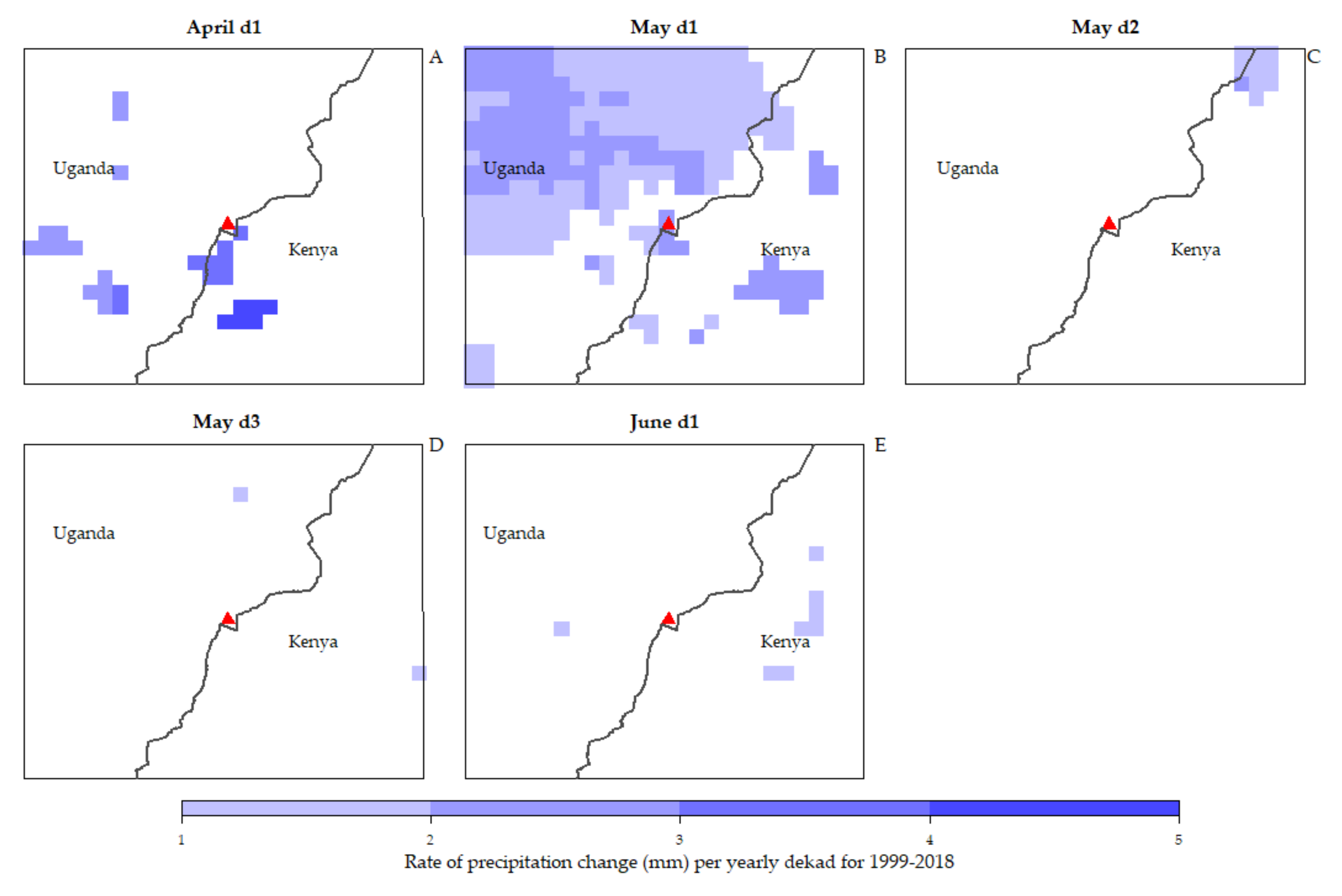
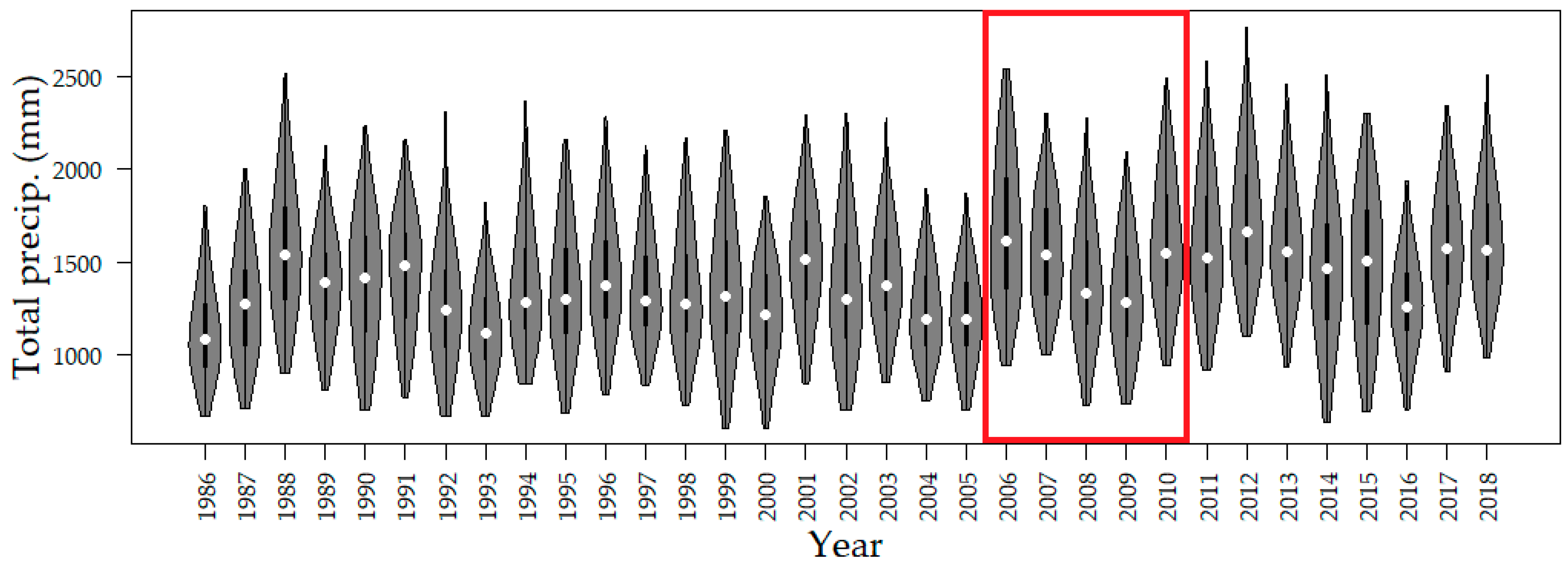
4.1.2. Precipitation Variability in the MEE

The test for monotonic trends in precipitation revealed various patterns of consistently increasing (wetting) and decreasing (drying) precipitation within the MEE (Figure 6). Most of the areas experienced increased precipitation over the years and only negligible proportions of the study area became drier. The greatest proportions of land during which consistently wetter conditions prevailed include 1999–2018, 1986–2018 and 2001–2018 (82%, 58% and 38%, respectively). The areas experiencing change covered approximately 10,300, 7200 and 4800 km², respectively. These periods also showed the greatest magnitude of change in precipitation amount. Here, precipitation increased by at least 13, 4, and 5 mm per year for 1999–2018, 1986–2018 and 2001–2018 periods. In addition, about 27% of the MEE also experienced wetter conditions during 2008–2018.

There were very small portions of the MEE with wetter conditions during the earlier years in the analysis; 1.61% of land (200 km²) recorded wetter conditions in 1986–1996 while there was no significant increase in precipitation during the 1986–2005 and 1997–2007 periods. Consistently drier conditions were observed in two time periods (1986–1996 and 1986–2005). However, only negligible proportions of land (up to about 2%) experienced this change, although at substantial magnitudes of up to 9 mm per year. Different spatial patterns existed from 2000; significantly increasing precipitation in 2008–2018 was observed mostly on the Ugandan side, and the mountain forest and wetland reserves seemed to be excluded (Figure 6B). In 2001–2018, the changed pixels were mostly found within the mountain area, in the north and some areas in the west (Figure 6E). On the other hand, areas in the northeastern portion of the study area did not experience changes in precipitation during the 1986–2018 period (Figure 6F). Lastly, the 1999–2018 period had significant increases in total seasonal precipitation with an exception of a few eastern and southeastern portions of the MEE (Figure 6D). Overall, there was an increase in precipitation for most areas in the study area, with an increasing magnitude of change, especially in the post-2000 era.

The trend analysis for each dekad in the growing season found that, based on rates of change, the 2008–2018 period recorded the highest change in precipitation in April d1 and May d1, at rates of up to 13 mm per yearly dekad, see Figure 7). Areas where this change was experienced were located mostly in western MEE. An increase in precipitation was also recorded in April d2 in 2001–2018, June d3 in 1986–1996 and June d3 in 2008–2018. Negative trends in MEE precipitation were also observed in some dekads, mostly in 1986–2005. During this period, precipitation decreased in April d1, May d2 and June d1, at the rate of up to 3 mm per annual dekad.

Based on the proportions of land with significant change in precipitation, the study found that most of MEE precipitation significantly changed during May d1 in 1986–2018 (90%, 11,300 km²) and May d1 in 1999–2018 (43%, 5400 km², Figure 8). From these results, some patterns are clear. For the months of May and June, annual dekad precipitation increased significantly for all time periods, although at varying rates and proportions. Precipitation in most of the MEE was more stable in the earlier years in the study (as in 1986–1996) or generally depicted significant and consistently drier conditions (as in 1986–2005). Based on these results and those in Figure 6 above, it was necessary to conduct a breakpoint analysis to provide a better characterization of any specific spatio-temporal breaks in precipitation and greenness trends.

4.2. Breakpoint Analysis Results: bfast

While breakpoint analysis was performed for both 1986–2018 and 2001–2018 precipitation TS, no significant breaks were found in the former. Therefore, results from 2001–2018 are presented in this study.

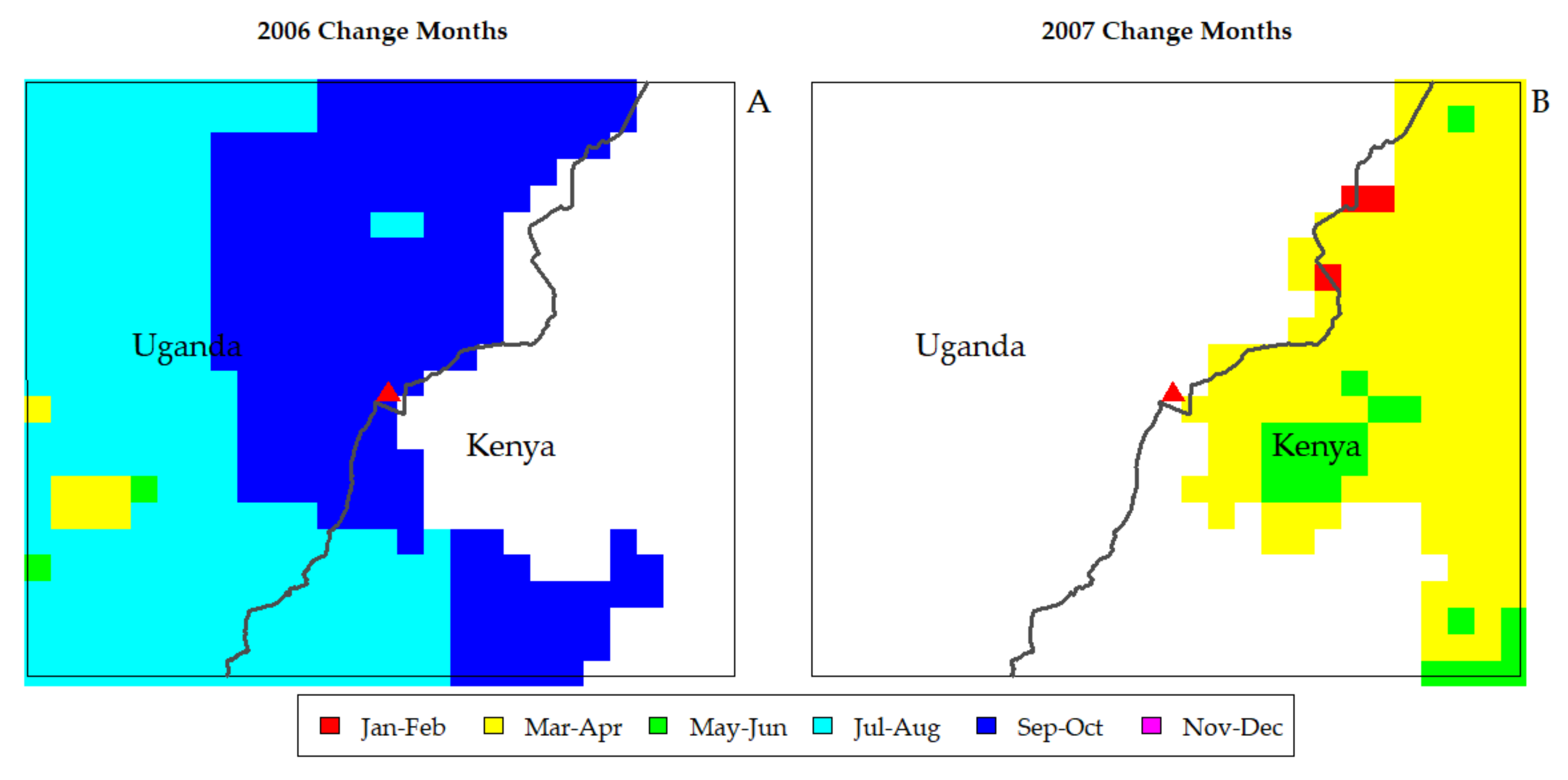
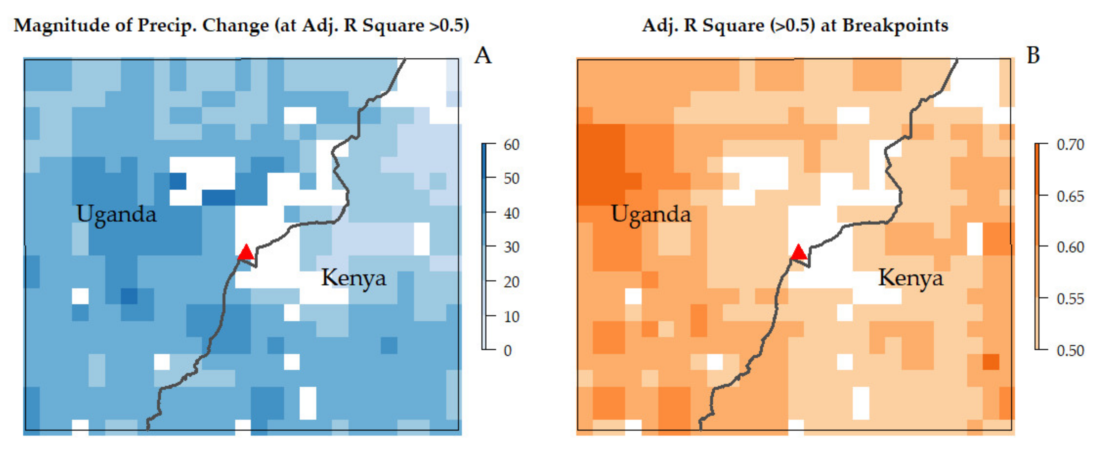
4.2.1. MEE Precipitation

The breakpoint analysis in bfast revealed no significant breaks in MEE average mean total monthly precipitation. However, breakpoints monitored for each pixel from January 2005 revealed very interesting patterns. In most configurations, the analysis revealed significant breakpoints in 2006 and 2007 for most of the MEE. To reduce the influence of post-change detection observations on change magnitude, the same analysis was performed for the period 2001–2008, with 2001–2004 set as the historical period. Therefore, change maps and statistics provided are based on this adjusted analysis. Precipitation changed significantly in the two years, with about 9800 km² (66% of the area) and 4800 km² (32%) of the MEE experiencing wetter conditions in 2006 and 2007, respectively (Figure 9). Most of the breakpoints in 2006 were detected in the months of July–October, while a great proportion of changes in 2007 were detected in March and April. Similar wetter conditions were detected in some locations in the months of May and June for both years. No drier conditions were detected. The magnitude of precipitation change ranged from approximately 10 to 53 mm during the monitored period (Figure 10A) and the bfast models used could explain up to 70% of the variance in the precipitation breakpoints (Figure 10B). Precipitation was also monitored sequentially for the period 2005–2018 and no breakpoints were detected except for a few pixels in 2005–2007.

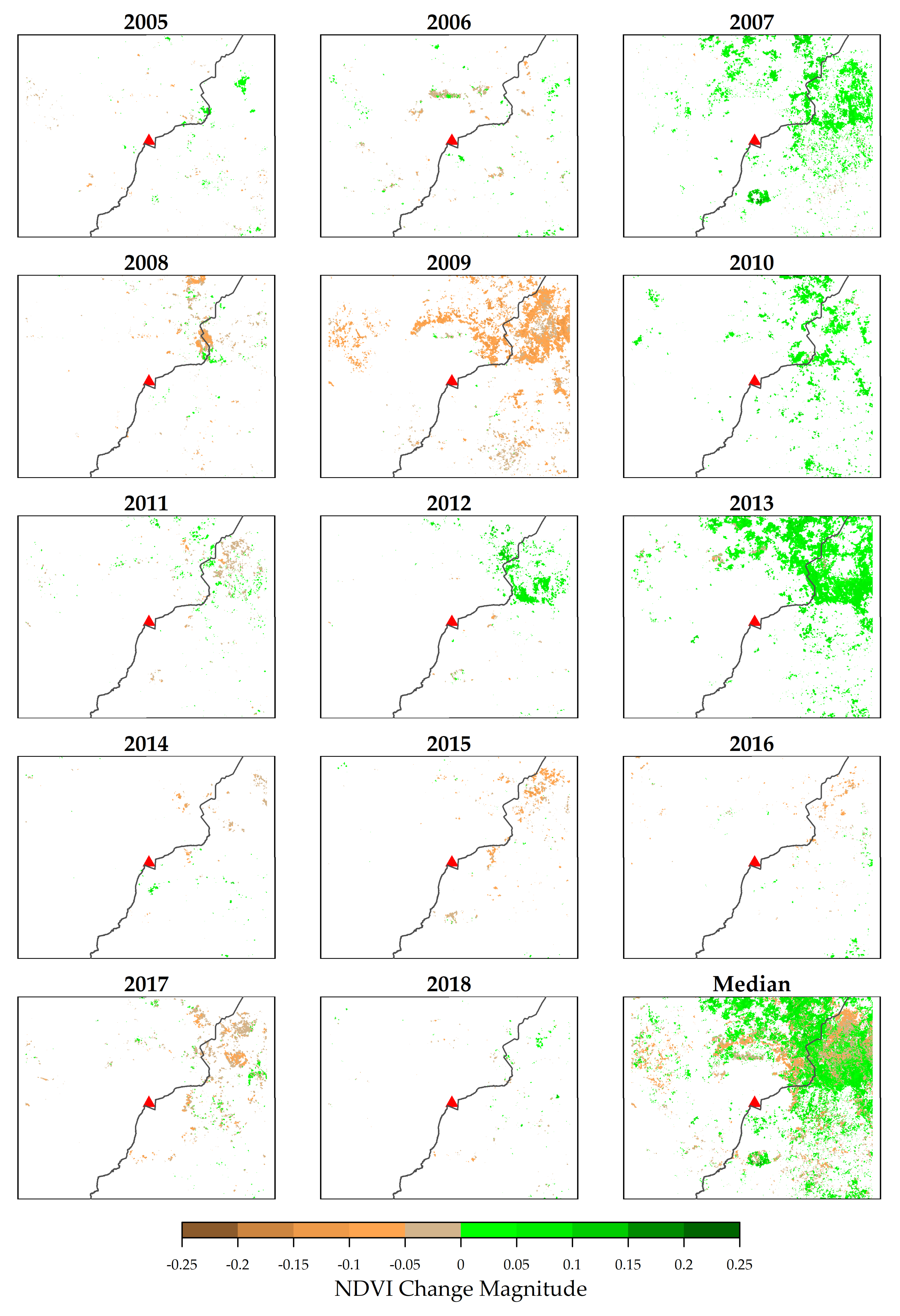
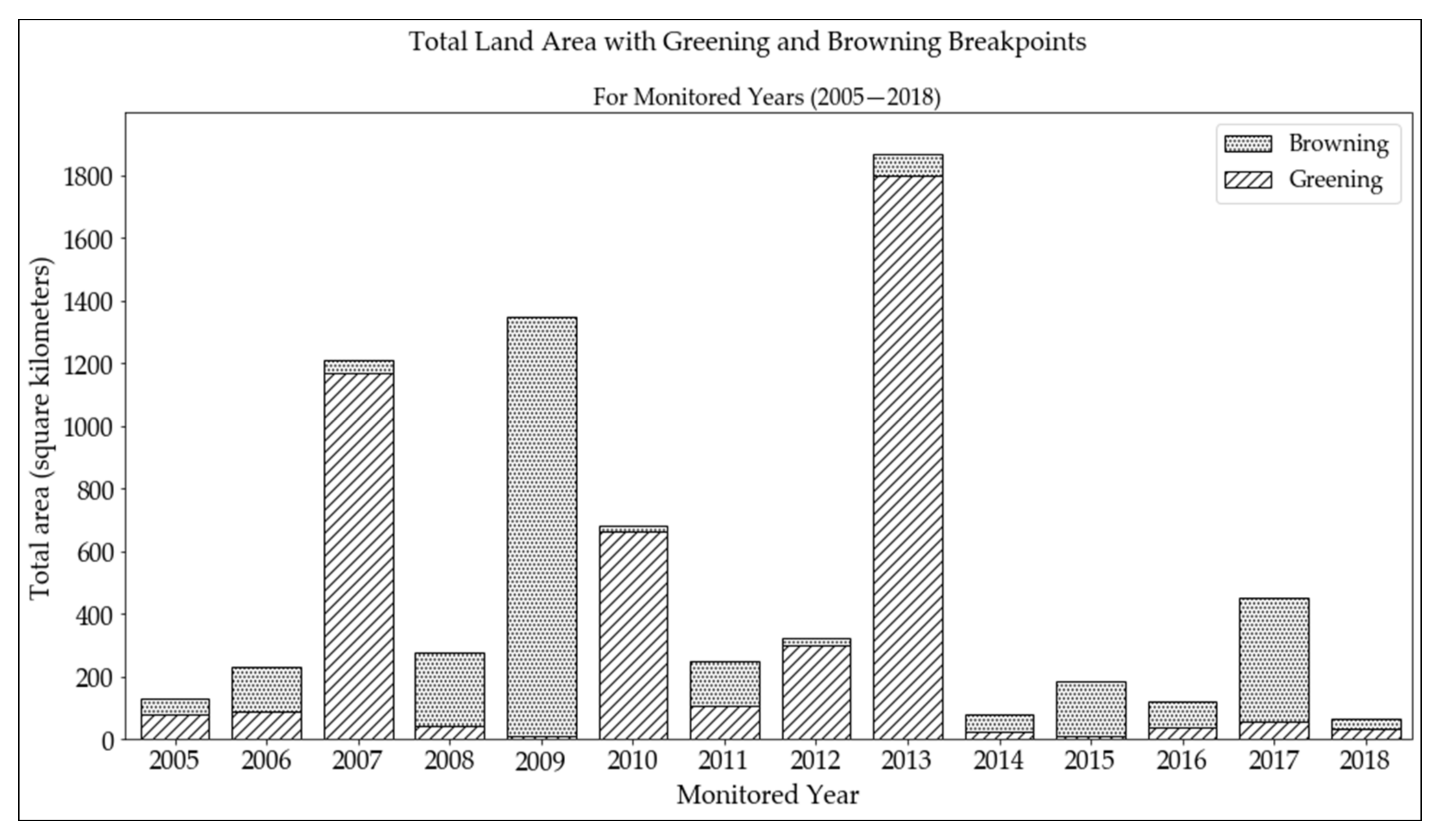
4.2.2. MEE Greenness

The analysis of breakpoints revealed that some significant breaks existed in the NDVI time series for each year (2005–2018). Having been sequentially monitored, the results include, for each monitored year, months when the breakpoints were observed, the magnitude of change at the breakpoints, the length of historical data used and adjusted R². In this analysis, only highly statistically significant changes (p < 0.05) are reported. This decision was based on two reasons: (i.) There were no ground data for validating results from sequentially monitored bfast. To ensure that only accurate results are reported, breakpoints from models with less than 50% adjusted R² were excluded. Thus, only breakpoints from models with average to high explanatory power were reported. This 50% threshold has been used elsewhere by Landmann and Dubovyk [6]. (ii.) Vegetation greenness in the MEE showed significant interannual variability. As such, to ensure a long-enough historical period used by ‘bfastSpatial’, the study excluded any breakpoints from models using a historical period of less than two years.

The ‘bfastSpatial’ model was able to detect changes in vegetation greenness, especially in the grasslands of the northeastern MEE (Figure 1 and Figure 11). The observed changes could be due to both natural factors (such as variability in precipitation) and/or human activities (for example, clearing of land for agriculture and settlement, deforestation for charcoal burning and construction etc.). The maximum magnitude of changes ranged from −0.24 and 0.21, thus indicating only subtle changes in the MEE vegetation. The breakpoints were detected in each of the years, but most of them were observed in 2013, 2007 and 2010 (greening) and 2009 and 2017 (browning), as shown in Figure 11. Overall, there were more areas where significant greening trends were detected compared to browning, with about 17% of the MEE (about 2500 km²) and 10% (about 1500 km²) showing greening and browning, respectively, over the monitoring period. These represent annual greening and browning rates of about 1.2% and 0.7%, respectively.

Based on the yearly changes, differentiated greening and browning patterns were observed during the monitoring period. Cumulatively, the greatest proportion of land with changed greenness was in 2013 in which significant breakpoints were observed in approximately 13% of the MEE (approximately 1850 km²). This was followed by 2009 (1350 km²), 2007 (1200 km²) and 2010 (650 km²) (Figure 12). For 2013, 2010 and 2007, the majority (over 95%) of the changed locations experienced greening. The year 2009 recorded browning in over 99% of the changed locations.

4.2.3. MEE Greenness vs Precipitation

There was an increase in precipitation in 2006 compared to previous years (Figure 13). There followed a steady decrease in 2007–2009 and finally an increase in 2010. Similar changes were observed in greenness during the five years. First, there was greening at most breakpoints in 2007 following the significant wetting in 2006. Significant browning followed, most of which occurred in 2009. This was also observable in an aspatial bfast breakpoint analysis performed on MEE mean NDVI, in which a sudden increase in NDVI was observed towards the end of 2006, followed by a consistently reducing trend until 2009/2010, in which another sudden increase was found (Figure 14). No significant breakpoints were found from a similar analysis using mean MEE precipitation. However, results from ‘bfastSpatial’ indicate that most of the MEE had very significant increases in precipitation in the second half of 2006 and the first half of 2007. Therefore, the corresponding changes in vegetation greenness can be attributed to this change in precipitation.

The significant and extensive browning observable mostly in 2009 (Figure 11) may be explained in terms of vegetation regaining its ‘normal’ greenness levels following sudden greening due to an above-normal precipitation. However, no significant breaks were found in precipitation around 2013, the year with the highest proportion of land with detected change in vegetation greenness. Thus, such browning and greening trends can be explained with regards to other factors, including temperature and anthropogenic activities that may have altered vegetation greenness during the monitoring period. The ‘bfastSpatial’ model did not find any significant breakpoints, in precipitation TS, in 2012. This may be due to the unstable historical data prior to the monitoring period. However, the violin plot (Figure 13) indicates that this year had some of the highest precipitation recordings. As such, there is a high chance that the greening following in 2013 was influenced by this increase in precipitation.

A visual inspection of these results in Google Earth Pro indicates that the subtle changes are indicative of various LULC changes. There was evidence of human settlement being introduced into the grasslands in the northeastern MEE. Information gathered from the field corroborates this finding and further explains the implications for landscape greenness. Inhabited by nomadic pastoralist communities, this part of the MEE is susceptible to degradation, especially when these communities move, driven by rainfall patterns, to settle within the grasslands. Based on fieldwork and data from Google Earth Pro, reduced natural vegetation and tree density were evident in these locations. In other instances, the new inhabitants converted natural vegetation to agriculture and, although this would result in environmental degradation, some planted crops were greener than the natural vegetation, and, therefore, these areas were shown to exhibit greening trends. In other locations outside of the grasslands, visible greening trends were indicative of some afforestation practices. Data from the field revealed that this kind of greening was driven by the cultivation of evergreen early maturing blue gum (Eucalyptus globulus) tree species, sometimes together with and other times in the place of the maize crop. This was especially common in the eastern and southeastern parts of the domain and parts of Uganda.

4.3. Accuracy Assessment

Validation of Man-Kendall and Sen’s slope results revealed an overall accuracy of 98.04% and user’s accuracies of 100%, 98% and 96.2% for browned, greened, and unchanged locations, respectively (

Table 2. Mann–Kendall and Sen’s slope accuracy assessment statistics.

	Browned	Greened	No Change	User’s Accuracy
Browned	50	0	0	100
Greened	0	49	1	98
No change	1	1	51	96.2
Producer’s Accuracy	98	98	98.1
Overall Accuracy				98.04

). Producer’s accuracies of 98% (for both browned and greened locations) and 98.1% (no change) were also obtained. The visual inspection of bfast results using Google Earth Pro also revealed that most of the detected subtle changes occurred. However, no more detailed information like year of change could be discerned due to the lack of available high-resolution imagery.

5. Discussion

5.1. Precipitation and Vegetation Change in the MEE

Climate change continues to affect economies in most developing nations, especially those relying heavily on natural processes for their livelihoods. Agriculture remains the backbone of many of these nations [76,77,78,79,80,81,82], yet agriculture’s vulnerability to climate change effects cannot be contested. Climate-related natural hazards, including extensive flooding, extended droughts [83], landslides [28] among others, have significantly impacted agricultural production and endangered lives. The frequency of these events shows an increasing trend [84,85], thus trapping many agriculture-dependent communities in an unending struggle for survival. Therefore, existing food insecurity in these developing nations can be attributed to their overreliance on rainfed agriculture [83]. Moreover, the high population growth and densities in these nations and elsewhere have translated into need for more agricultural land [28]. Coupled with political interference and corruption among forest park and reserve staff, this need for more land has resulted in forest encroachment and deforestation as ecologically fragile land is cleared for agriculture and settlement [28,29,30,31,32]. Therefore, understanding the major drivers of landscape change is an important first step to inform better decisions to simultaneously conserve the natural environment and improve the livelihoods dependent on it. First, being able to separate nature- from human-induced landscape changes would be valuable in this endeavor.

Changes in the landscape occur at varying rates and magnitudes across space and time, from very subtle tree damages to forest clearings [49]. In this study, two major forms of landscape change—browning (areas of declining vegetation) and greening (areas of increasing vegetation) [12]—were studied. The results show that MEE greenness exhibited substantial variability, and some form of the greening and browning change was recorded each year. As expected, these changes varied by scale, with the highest proportions of greened and browned locations observed over the growing season rather than any of the individual 16-day periods. Importantly, there was a lot of activity in areas bordering the mountain forest, as expected. Clearly, both greening and browning trends were observable, particularly on the Kenya side. Significant deforestation occurred as a result of encroaching fertile land on the high slopes of the mountain, for agriculture and settlement (examples in Figure 15). This finding has been reported in previous studies [27,28]. The Shamba system, thought of as a win-win arrangement, enabled local communities to farm in protected areas while tending to the growing trees in their early stages of growth [27]. This was a government effort originally meant to convert native to plantation forests and later to replant trees on harvested forest land. However, the Shamba system farms overlap with plantation forest and bamboo vegetation thus making it more difficult to conclusively identify, characterize and quantify the nature and magnitude of LULC change, especially by the use of traditional classification and change detection methods [27]. The significant and consistent browning in the southwestern MEE are attributed to the conversion of the Namatala wetland to agriculture (mostly paddy rice farming) and settlement (due to the growth of Mbale town) [75]. Since the early 2000s, 80–90% of this wetland has been converted. The wetland area is an Important Bird Area (IBA) [86] and therefore the reported LULC conversion caused many nature–human and human–human conflicts, including, respectively, bird poisoning and competition among people to own and utilize the wetland.

Disentangling nature- from human-induced vegetation change is an important yet complex task. In this study, patterns of change in precipitation varied with the TS duration (33-, 11-, 20- and 18-years) and resolution (dekad, seasonal). Previous studies indicated that precipitation in the area exhibited significant temporal variability, with both positive [63] and negative [80] trends observed over time. It can be inferred that precipitation had changed more (increased) over the period after 2000 than earlier. This implies that some of the vegetation greening and browning should be linked to this MEE wetting. This is true for the period 2006–2010, where bfast reveals that greening and browning events in the MEE follow significant wetting and drying events. However, a visual interpretation of Mann–Kendall analysis maps for both MODIS NDVI and CHIRPS precipitation did not show much similarity. Besides, bfast did not reveal any breakpoints in precipitation around 2013, the year when most breakpoints in greenness were detected. While this may be a fault in the bfast model used (because of, for instance, instability in historical data used), precipitation alone may not be a reliable predictor of vegetation change [49]. Davenport and Nichols [22] concluded that the NDVI–precipitation relationship varies both spatially and temporally, is not linear, generally exhibits a three-month lag, and depends on underlying LULC types. Therefore, it is likely that these complex relationships were not well revealed in both analyses in this study. Besides, the observed greening and browning patterns may be driven by other climate factors (such as temperature), which were not examined in this study, due in part to data unavailability for the MEE. Moreover, the spatial scale mismatch between the CHIRPS and MODIS data make more quantitative comparisons challenging.

Visual inspections of the results from both analyses revealed the applicability of Mann–Kendall and bfast methods in detecting changes in vegetation greenness. Most people in the MEE are small-scale farmers, owning sometimes less than an acre (0.4 hectares) of land. This represents less than 10 percent of the pixel size used (250 by 250-meter MODIS), meaning that some subtle land conversions were missed. The choice to use these data was necessitated by the frequent availability of MODIS NDVI data. The ability of Mann–Kendall and bfast in delineating areas of change in the MEE using this coarse imagery is important, as free finer RS imagery like Landsat is limited by both cloud cover across tropical regions and their coarse temporal resolutions. Looking forward, combining Sentinel-2 and Landsat imagery may help address this issue, but this will not resolve the problem for historical studies like this one.

The use of Mann–Kendall and bfast algorithms proved to be a valuable integration. Mann–Kendall performed well in mapping locations that had experienced significant change in the entire TS (2001–2018). Consistently greened and browned locations were mapped with high confidence (95% significance level) and similar patterns existed for both 16-day and average growing season periods: significant and consistent browning in southwestern MEE and greening elsewhere. The best and most accurate results were obtained using average growing season NDVI TS. Here, browned locations (especially around mountain boundaries and southwestern MEE) and greening elsewhere were clearly demarcated. This indicates that the growing season period, rather than the shorter 16-day period, is the best temporal scale for monitoring vegetation change in the MEE. bfast on the other hand performed well in mapping changed greenness locations for sequentially monitored periods from 2005 to 2018. This part of the analysis revealed only subtle changes in vegetation greenness in most locations, indicative of vegetation degradation rather than deforestation [70]. Importantly, areas with breakpoints across multiple years were effectively identified, a finding that would likely be omitted if using traditional post-classification change detection methods. These findings demonstrate that the process of vegetation greening and browning can be studied more thoroughly by fusing these two methods. Using Mann–Kendall and Sen’s Slope, one can assess and quantify monotonic trends in their TS to get the general picture in the series. This can be complimented with an assessment of the temporal occurrence of significant breaks in the series using bfast. Using this integrated approach, vegetation greening and browning can be fully characterized and understood to provide more information for better decision making.

5.2. Sources of Uncertainty

Due to a lack of ground precipitation measurements, the present study did not validate the CHIRPS data over the MEE. The GHCN data [87] would potentially be used, but only one data point existed in the study area and was therefore deemed insufficient for this task. While this is a potential source of uncertainty, these data have been used extensively in similar studies. Moreover, CHIRPS data are based on ground station data since they are created through “smart interpolation” procedures that incorporate both satellite information and gauge data [53] thus making daily CHIRPS imprecise, and reliable only at dekad or higher aggregations. Validation of bfast results was also not possible due to a similar lack of data. Frequent, high-resolution imagery was not freely available to download and process, and the study relied on imagery from Google Earth Pro which had a lot of spatial and temporal gaps. While no accuracy statistics were calculated for these results, the results were interpreted based in part on data collected from the MEE field study.

6. Conclusions

The MEE of eastern Uganda and western Kenya was found to exhibit significant variability in vegetation dynamics and precipitation regimes. This variability was attributed to the existing LULC orientation especially in eastern MEE and climate change and variability. As such, it is highly probable that analysis of only a few images to ascertain MEE landscape change would yield inconsistent results. In this study, greening and browning in the MEE was examined using both TS trend and breakpoint analysis methods. The MEE had experienced significant and persistent greening and browning at different time scales and this change was attributed to both natural factors (including changing precipitation) and anthropogenic factors (especially the vegetation-to-cropland conversion). The southwestern MEE had consistently browned due to the conversion of the Namatala swamp to paddy rice farming and settlement. A lot of activity was also observed around the mountain forest boundary as people encroached and converted the forest LULC to agriculture and settlement. There were breakpoints in the vegetation greenness TS, particularly in the savanna and grassland land covers in northeastern MEE. The breakpoints were detected in each of the monitored years (2005–2018), but most of them were observed in 2013, 2007 and 2010 (greening) and 2009 and 2017 (browning). The study also concluded that MEE precipitation had significantly changed (increased) in the post-2000 era. More specifically, total precipitation significantly increased in 2006 and 2009–2010 with a consistently decreasing trend in between. We therefore concluded that these precipitation changes influenced significant greening and browning patterns observed in the same period. The greenness–precipitation relationship was weak in other periods as greening and browning changes were not strongly influenced by changing precipitation. This may be attributed to the complex nature of the MEE landscape and/or the spatial and temporal scale mismatch between MODIS NDVI and CHIRPS precipitation data. The integration of Mann–Kendall, Sen’s slope and bfast proved useful in comprehensively characterizing recent changes in vegetation greenness within the MEE. Having a comprehensive description of vegetation change is an important first step, especially for such a variable landscape, to effect policy changes aimed at simultaneously conserving the environment and improving livelihoods that are dependent on it.

References

1. Gemitzi, A.; Banti, M.; Lakshmi, V. Vegetation greening trends in different land use types: Natural variability versus human-induced impacts in Greece. Environ. Earth Sci. 2019, 78, 1–10. [Google Scholar] [CrossRef]
2. Alavipanah, S.; Wegmann, M.; Qureshi, S.; Weng, Q.; Koellner, T. The role of vegetation in mitigating urban land surface temperatures: A case study of Munich, Germany during the warm season. Sustainability 2015, 7, 4689–4706. [Google Scholar] [CrossRef] [Green Version]
3. Forzieri, G.; Alkama, R.; Miralles, D.G.; Cescatti, A. Response to Comment on “Satellites reveal contrasting responses of regional climate to the widespread greening of Earth”. Science 2018, 360, 1180–1184. [Google Scholar] [CrossRef] [PubMed] [Green Version]
4. Ballantyne, A.; Smith, W.; Anderegg, W.; Kauppi, P.; Sarmiento, J.; Tans, P.; Shevliakova, E.; Pan, Y.; Poulter, B.; Anav, A.; et al. Accelerating net terrestrial carbon uptake during the warming hiatus due to reduced respiration. Nat. Clim. Chang. 2017, 7, 148–152. [Google Scholar] [CrossRef]
5. Pan, N.; Feng, X.; Fu, B.; Wang, S.; Ji, F.; Pan, S. Increasing global vegetation browning hidden in overall vegetation greening: Insights from time-varying trends. Remote Sens. Environ. 2018, 214, 59–72. [Google Scholar] [CrossRef]
6. Landmann, T.; Dubovyk, O. Spatial analysis of human-induced vegetation productivity decline over eastern Africa using a decade (2001-2011) of medium resolution MODIS time-series data. Int. J. Appl. Earth Obs. Geoinf. 2014, 33, 76–82. [Google Scholar] [CrossRef]
7. Zhu, Z.; Piao, S.; Myneni, R.B.; Huang, M.; Zeng, Z.; Canadell, J.G.; Ciais, P.; Sitch, S.; Friedlingstein, P.; Arneth, A.; et al. Greening of the Earth and its drivers. Nat. Clim. Chang. 2016, 6, 791–795. [Google Scholar] [CrossRef]
8. Olsson, L.; Eklundh, L.; Ardö, J. A recent greening of the Sahel - Trends, patterns and potential causes. J. Arid Environ. 2005, 63, 556–566. [Google Scholar] [CrossRef]
9. Le Quéré, C.; Raupach, M.R.; Canadell, J.G.; Marland, G.; Bopp, L.; Ciais, P.; Conway, T.J.; Doney, S.C.; Feely, R.A.; Foster, P.; et al. Trends in the sources and sinks of carbon dioxide. Nat. Geosci. 2009, 2, 831–836. [Google Scholar] [CrossRef]
10. Mishra, N.B.; Mainali, K.P. Greening and browning of the Himalaya: Spatial patterns and the role of climatic change and human drivers. Sci. Total Environ. 2017, 587–588, 326–339. [Google Scholar] [CrossRef]
11. Fensholt, R.; Langanke, T.; Rasmussen, K.; Reenberg, A.; Prince, S.D.; Tucker, C.; Scholes, R.J.; Le, Q.B.; Bondeau, A.; Eastman, R.; et al. Greenness in semi-arid areas across the globe 1981-2007—An Earth Observing Satellite based analysis of trends and drivers. Remote Sens. Environ. 2012, 121, 144–158. [Google Scholar] [CrossRef]
12. Murthy, K.; Bagchi, S. Spatial patterns of long-term vegetation greening and browning are consistent across multiple scales: Implications for monitoring land degradation. L. Degrad. Dev. 2018, 29, 2485–2495. [Google Scholar] [CrossRef]
13. Chamaille-Jammes, S.; Fritz, H.; Murindagomo, F. Spatial patterns of the NDVI-rainfall relationship at the seasonal and interannual time scales in an African savanna. Int. J. Remote Sens. 2006, 27, 5185–5200. [Google Scholar] [CrossRef]
14. Tucker, C.J. Red and photographic infrared linear combinations for monitoring vegetation. Remote Sens. Environ. 1979, 8, 127–150. [Google Scholar] [CrossRef] [Green Version]
15. Vrieling, A.; de Beurs, K.M.; Brown, M.E. Variability of African farming systems from phenological analysis of NDVI time series. Clim. Change 2011, 109, 455–477. [Google Scholar] [CrossRef] [Green Version]
16. Verbesselt, J.; Hyndman, R.; Zeileis, A.; Culvenor, D. Phenological change detection while accounting for abrupt and gradual trends in satellite image time series. Remote Sens. Environ. 2010, 114, 2970–2980. [Google Scholar] [CrossRef] [Green Version]
17. Guan, Q.; Yang, L.; Pan, N.; Lin, J.; Xu, C.; Wang, F.; Liu, Z. Greening and browning of the Hexi Corridor in northwest China: Spatial patterns and responses to climatic variability and anthropogenic drivers. Remote Sens. 2018, 10, 1270. [Google Scholar] [CrossRef] [Green Version]
18. Emmett, K.D.; Renwick, K.M.; Poulter, B. Disentangling Climate and Disturbance Effects on Regional Vegetation Greening Trends. Ecosystems 2019, 22, 873–891. [Google Scholar] [CrossRef] [Green Version]
19. Malo, A.R.; Nicholson, S.E. A study of rainfall and vegetation dynamics in the African Sahel using normalized difference vegetation index. J. Arid Environ. 1990, 19, 1–24. [Google Scholar] [CrossRef]
20. Schmidt, H.; Gitelson, A. Temporal and spatial vegetation cover changes in Israeli transition zone: AVHRR-based assessment of rainfall impact. Int. J. Remote Sens. 2000, 21, 997–1010. [Google Scholar] [CrossRef]
21. Fabricante, I.; Oesterheld, M.; Paruelo, J.M. Annual and seasonal variation of NDVI explained by current and previous precipitation across Northern Patagonia. J. Arid Environ. 2009, 73, 745–753. [Google Scholar] [CrossRef]
22. Davenport, M.L.; Nicholson, S.E. On the relation between rainfall and the Normalized Difference Vegetation Index for diverse vegetation types in East Africa. Int. J. Remote Sens. 1993, 14, 2369–2389. [Google Scholar] [CrossRef]
23. Farrar, T.J.; Nicholson, S.E.; Lare, A.R. The influence of soil type on the relationships between NDVI, rainfall, and soil moisture in semiarid Botswana. I. NDVI response to rainfall. Remote Sens. Environ. 1994, 50, 107–120. [Google Scholar] [CrossRef]
24. Guzha, A.C.; Rufino, M.C.; Okoth, S.; Jacobs, S.; Nóbrega, R.L.B. Impacts of land use and land cover change on surface runoff, discharge and low flows: Evidence from East Africa. J. Hydrol. Reg. Stud. 2018, 15, 49–67. [Google Scholar] [CrossRef]
25. Maitima, J.M.; Mugatha, S.M.; Reid, R.S.; Gachimbi, L.N.; Majule, A.; Lyaruu, H.; Pomery, D.; Mathai, S.; Mugisha, S. The linkages between land use change, land degradation and biodiversity across East Africa. African J. Agric. Res. 2009, 3, 310–325. [Google Scholar]
26. Vrieling, A.; De Leeuw, J.; Said, M.Y. Length of growing period over africa: Variability and trends from 30 years of NDVI time series. Remote Sens. 2013, 5, 982–1000. [Google Scholar] [CrossRef] [Green Version]
27. Petursson, J.G.; Vedeld, P.; Sassen, M. An institutional analysis of deforestation processes in protected areas: The case of the transboundary Mt. Elgon, Uganda and Kenya. For. Policy Econ. 2013, 26, 22–33. [Google Scholar] [CrossRef]
28. Mugagga, F.; Kakembo, V.; Buyinza, M. Land use changes on the slopes of Mount Elgon and the implications for the occurrence of landslides. Catena 2012, 90, 39–46. [Google Scholar] [CrossRef]
29. Muhweezi, A.B.; Sikoyo, G.M.; Chemonges, M. Introducing a Transboundary Ecosystem Management Approach in the Mount Elgon Region. Mt. Res. Dev. 2007, 27, 215–219. [Google Scholar] [CrossRef]
30. EAC; UNEP; GRID-Arendal. Sustainable Mountain Development in East Africa in a Changing Climate; EAC: Arusha, Tanzania, 2016; ISBN 9788277011547. [Google Scholar]
31. Nakakaawa, C.; Moll, R.; Vedeld, P.; Sjaastad, E.; Cavanagh, J. Collaborative resource management and rural livelihoods around protected areas: A case study of Mount Elgon National Park, Uganda. For. Policy Econ. 2015, 57, 1–11. [Google Scholar] [CrossRef]
32. Bamutaze, Y.; Tenywa, M.M.; Majaliwa, M.; Vanacker, V.; Bagoora, F.; Magunda, M.; Obando, J.; Wasige, J.E. Infiltration characteristics of volcanic sloping soils on Mount Elgon, Eastern Uganda. Catena 2010, 80. [Google Scholar] [CrossRef]
33. Myhren, S.M. Rural Livelihood and Forest Management in Mount Elgon, Kenya; Norwegian University of Life Sciences: Ås, Norway, 2007. [Google Scholar]
34. Barasa, B.; Kakembo, V. The Impact of Land Use/Cover Change on Soil Organic Carbon and Its Implication on Food Security and Climate Change Vulnerability on the Slopes of Mt. Elgon, Eastern Uganda; Nelson Mandela Metropolitan University: Port Elizabeth, South Africa, 2013. [Google Scholar]
35. Mugagga, F.; Nagasha, B.; Barasa, B.; Buyinza, M. The Effect of Land Use on Carbon Stocks and Implications for Climate Variability on the Slopes of Mount Elgon, Eastern Uganda. Int. J. Reg. Dev. 2015, 2, 58. [Google Scholar] [CrossRef]
36. Sulla-Menashe, D.; Friedl, M.A. User Guide to Collection 6 MODIS Land Cover (MCD12Q1 and MCD12C1) Product; USGS: Reston, VA, USA, 2018. [Google Scholar]
37. Gómez, C.; White, J.C.; Wulder, M.A. Optical remotely sensed time series data for land cover classification: A review. ISPRS J. Photogramm. Remote Sens. 2016, 116, 55–72. [Google Scholar] [CrossRef] [Green Version]
38. Woodcock, C.E.; Allen, R.; Anderson, M.; Belward, A.; Bindschadler, R.; Cohen, W.; Gao, F.; Goward, S.N.; Helder, D.; Helmer, E.; et al. Free Access to Landsat Imagery. Science 2008, 320, 1011–1012. [Google Scholar] [CrossRef] [PubMed]
39. Badjana, H.M.; Helmschrot, J.; Selsam, P.; Wala, K.; Flugel, W.-A.; Afouda, A.; Akpagana, K. Land Cover Changes assessment using object-based image analysis in the Binah River watereshed (Togo and Benin). Earth Sp. Sci. 2015, 2, 403–416. [Google Scholar] [CrossRef] [Green Version]
40. Bradley, B.A.; Jacob, R.W.; Hermance, J.F.; Mustard, J.F. A curve fitting procedure to derive inter-annual phenologies from time series of noisy satellite NDVI data. Remote Sens. Environ. 2007, 106, 137–145. [Google Scholar] [CrossRef]
41. Hermance, J.F.; Jacob, R.W.; Bradley, B.A.; Mustard, J.F. Extracting phenological signals from multiyear AVHRR NDVI time series: Framework for applying high-order annual splines with roughness damping. IEEE Trans. Geosci. Remote Sens. 2007, 45, 3264–3276. [Google Scholar] [CrossRef]
42. Crist, E.P.; Cicone, R.C. A Physically-Based Transformation of Thematic Mapper Data-The TM Tasseled Cap. IEEE Trans. Geosci. Remote Sens. 1984, 22, 256–263. [Google Scholar] [CrossRef]
43. Anyamba, A.; Eastman, J.R. Interannual variability of ndvi over africa and its relation to el niño/southern oscillation. Int. J. Remote Sens. 1996, 17, 2533–2548. [Google Scholar] [CrossRef]
44. Mann, H.B. Nonparametric Tests Against Trend. Econometrica 1945, 13, 245–259. [Google Scholar] [CrossRef]
45. Lamchin, M.; Lee, W.K.; Jeon, S.W.; Wang, S.W.; Lim, C.H.; Song, C.; Sung, M. Long-term trend of and correlation between vegetation greenness and climate variables in Asia based on satellite data. MethodsX 2018, 5, 803–807. [Google Scholar] [CrossRef]
46. Khambhammettu, P. Annual Groundwater Monitoring Report, Appendix D - Mann-Kendall Analysis for the Fort Ord Site; HydroGeoLogic, Inc.: Monterey County, CA, USA, 2005. [Google Scholar]
47. Sen, P.K. Estimates of the Regression Coefficient Based on Kendall’s Tau. J. Am. Stat. Assoc. 1968, 63, 1379–1389. [Google Scholar] [CrossRef]
48. Alcaraz-Segura, D.; Chuvieco, E.; Epstein, H.E.; Kasischke, E.S.; Trishchenko, A. Debating the greening vs. browning of the North American boreal forest: Differences between satellite datasets. Glob. Chang. Biol. 2010, 16, 760–770. [Google Scholar] [CrossRef]
49. Morrison, J.; Higginbottom, T.P.; Symeonakis, E.; Jones, M.J.; Omengo, F.; Walker, S.L.; Cain, B. Detecting vegetation change in response to confining elephants in forests using MODIS time-series and BFAST. Remote Sens. 2018, 10, 1075. [Google Scholar] [CrossRef] [Green Version]
50. Hamilton, A.C.; Perrott, R.A. A study of altitudinal zonation in the montane forest belt of Mt. Elgon, Kenya/Uganda. Plant Ecol. 1981, 45, 107–125. [Google Scholar] [CrossRef]
51. The Struggle over Land in Africa: Conflicts, Politics and Change; Anseeuw, W.; Alden, C. (Eds.) HSRC Press: Cape Town, South Africa, 2010; ISBN 9780796923226. [Google Scholar]
52. Doumenge, C.; Gilmour, D.; Pérez, M.R.; Blockhus, J. Tropical Montane Cloud Forests: Conservation Status and Management Issues. In Tropical Montane Cloud Forests; Springer: New York, NY, USA, 1995; pp. 24–37. [Google Scholar]
53. Funk, C.; Peterson, P.; Landsfeld, M.; Pedreros, D.; Verdin, J.; Shukla, S.; Husak, G.; Rowland, J.; Harrison, L.; Hoell, A.; et al. The climate hazards infrared precipitation with stations—A new environmental record for monitoring extremes. Sci. Data 2015, 2, 1–21. [Google Scholar] [CrossRef] [PubMed] [Green Version]
54. Okello, S.V.; Nyunja, R.O.; Netondo, G.W.; Onyango, J.C. Ethnobotanical study of medicinal plants used by the Sabaots of Mt. Elgon, Kenya. African J. Tradit. Contemp. Altern. Med. 2010, 7, 1–10. [Google Scholar] [CrossRef] [PubMed] [Green Version]
55. Musau, J.; Sang, J.; Gathenya, J.; Luedeling, E. Hydrological responses to climate change in Mt. Elgon watersheds. J. Hydrol. Reg. Stud. 2015, 3, 233–246. [Google Scholar] [CrossRef] [Green Version]
56. Didan, K. MOD13Q1 MODIS/Terra Vegetation Indices 16-Day L3 Global 250m SIN Grid V006; NASA EOSDIS Land Processes DAAC: Sioux Falls, SD, USA, 2015. [Google Scholar]
57. AppEEARS. AppEEARS Team Application for Extracting and Exploring Analysis Ready Samples (AppEEARS); LP DAAC: Sioux Falls, SD, USA, 2019. [Google Scholar]
58. USGS Landsat Satellite Missions. Available online: https://www.usgs.gov/land-resources/nli/landsat/landsat-satellite-missions?qt-science_support_page_related_con=2#qt-science_support_page_related_con (accessed on 12 May 2020).
59. Hawinkel, P.; Thiery, W.; Lhermitte, S.; Swinnen, E.; Verbist, B.; Van Orshoven, J.; Muys, B. Vegetation response to precipitation variability in East Africa controlled by biogeographical factors. J. Geophys. Res. Biogeosci. 2016, 121, 2422–2444. [Google Scholar] [CrossRef] [Green Version]
60. Gorelick, N.; Hancher, M.; Dixon, M.; Ilyushchenko, S.; Thau, D.; Moore, R. Google Earth Engine: Planetary-scale geospatial analysis for everyone. Remote Sens. Environ. 2017, 202, 18–27. [Google Scholar] [CrossRef]
61. Georganos, S.; Abdi, A.M.; Tenenbaum, D.E.; Kalogirou, S. Examining the NDVI-rainfall relationship in the semi-arid Sahel using geographically weighted regression. J. Arid Environ. 2017, 146, 64–74. [Google Scholar] [CrossRef]
62. Chen, C.; Li, T.; Li, J.; Fu, W.; Wang, G. Vegetation Change Analyses Considering Climate Variables and Anthropogenic Variables in the Three-River Headwaters Region. EPiC Ser. Eng. 2018, 3, 419–427. [Google Scholar]
63. Muthoni, F.K.; Odongo, V.O.; Ochieng, J.; Mugalavai, E.M.; Mourice, S.K.; Hoesche-Zeledon, I.; Mwila, M.; Bekunda, M. Long-term spatial-temporal trends and variability of rainfall over Eastern and Southern Africa. Theor. Appl. Climatol. 2019, 137, 1869–1882. [Google Scholar] [CrossRef] [Green Version]
64. Qualtrics LLC. Qualtrics; Qualtrics: Provo, UT, USA, 2019. [Google Scholar]
65. R Core Team. R: A Language and Environment for Statistical Computing; R Core Team: Vienna, Austria, 2018. [Google Scholar]
66. De Beurs, K.M.; Henebry, G.M. A land surface phenology assessment of the northern polar regions using MODIS reflectance time series. Can. J. Remote Sens. 2010, 36, S87–S110. [Google Scholar] [CrossRef]
67. Google LLC. Google Earth Pro; Google LLC: Menlo Park, CA, USA, 2020. [Google Scholar]
68. Verbesselt, J.; Zeileis, A.; Herold, M. Near real-time disturbance detection using satellite image time series. Remote Sens. Environ. 2012, 123, 98–108. [Google Scholar] [CrossRef]
69. Smith, V.; Portillo-Quintero, C.; Sanchez-Azofeifa, A.; Hernandez-Stefanoni, J.L. Assessing the accuracy of detected breaks in Landsat time series as predictors of small scale deforestation in tropical dry forests of Mexico and Costa Rica. Remote Sens. Environ. 2019, 221, 707–721. [Google Scholar] [CrossRef]
70. DeVries, B.; Verbesselt, J.; Kooistra, L.; Herold, M. Robust monitoring of small-scale forest disturbances in a tropical montane forest using Landsat time series. Remote Sens. Environ. 2015, 161, 107–121. [Google Scholar] [CrossRef]
71. Verbesselt, J.; Herold, M.; Hyndman, R.; Zeileis, A.; Culvenor, D. A robust approach for phenological change detection within satellite image time series. In Proceedings of the 2011 6th International Workshop on the Analysis of Multi-Temporal Remote Sensing Images, Multi-Temp 2011 - Proceedings, Trento, Italy, 12–14 July 2011; pp. 41–44. [Google Scholar]
72. Verbesselt, J.; Hyndman, R.; Newnham, G.; Culvenor, D. Detecting trend and seasonal changes in satellite image time series. Remote Sens. Environ. 2010, 114, 106–115. [Google Scholar] [CrossRef]
73. Foody, G.M. Status of land cover classification accuracy assessment. Remote Sens. Environ. 2002, 80, 185–201. [Google Scholar] [CrossRef]
74. Kennedy, R.E.; Yang, Z.; Cohen, W.B. Detecting trends in forest disturbance and recovery using yearly Landsat time series: 1. LandTrendr - Temporal segmentation algorithms. Remote Sens. Environ. 2010, 114, 2897–2910. [Google Scholar] [CrossRef]
75. Ministry of Water and Environment Uganda. Uganda Wetlands Atlas; Ministry of Water and Environment Uganda: Kampala, Uganda, 2016; Volume II.
76. FEWS Net. Kenya Food Security Brief; USAID: Washington, DC, USA, 2013. [Google Scholar]
77. Getachew Tesfaye Ayehu, S.A. Land Suitability Analysis for Rice Production: A GIS Based Multi-Criteria Decision Approach. Am. J. Geogr. Inf. Syst. 2015, 4, 95–104. [Google Scholar]
78. UNEP. Green Economy Sector Study on Agriculture in Kenya; UNEP: Nairobi, Kenya, 2015. [Google Scholar]
79. Salami, A.O.; Kamara, A.B.; Brixiova, Z. Smallholder Agriculture in East Africa: Trends, Constraints and Opportunities. In Working Paper Series; African Development Bank Group: Abidjan, Côte d’Ivoire, 2010. [Google Scholar]
80. Wanyama, D.; Koti, F. A Spatial Analysis of Climate Change Effects on Maize Productivity in Kenya; University of North Alabama: Florence, AL, USA, 2017. [Google Scholar]
81. Wanyama, D.; Mighty, M.; Sim, S.; Koti, F. A spatial assessment of land suitability for maize farming in Kenya. Geocarto Int. 2019. [Google Scholar] [CrossRef]
82. NAAIAP; KARI. Soil Suitability Evaluation for Maize Production in Kenya; Ministry of Agriculture Kenya: Nairobi, Kenya, 2014.
83. Kotikot, S.M.; Flores, A.; Griffin, R.E.; Sedah, A.; Nyaga, J.; Mugo, R.; Limaye, A.; Irwin, D.E. Mapping threats to agriculture in East Africa: Performance of MODIS derived LST for frost identification in Kenya’s tea plantations. Int. J. Appl. Earth Obs. Geoinf. 2018, 72, 131–139. [Google Scholar] [CrossRef]
84. Li, C.; Chai, Y.; Yang, L.; Li, H. Spatio-temporal distribution of flood disasters and analysis of influencing factors in Africa. Nat. Hazards 2016, 82, 721–731. [Google Scholar] [CrossRef]
85. Ayugi, B.; Tan, G.; Rouyun, N.; Zeyao, D.; Ojara, M.; Mumo, L.; Babaousmail, H.; Ongoma, V. Evaluation of meteorological drought and flood scenarios over Kenya, East Africa. Atmosphere 2020, 11, 307. [Google Scholar] [CrossRef] [Green Version]
86. BirdLife International Important Bird and Biodiversity Areas (IBAs). Available online: https://www.birdlife.org/worldwide/programme-additional-info/important-bird-and-biodiversity-areas-ibas (accessed on 1 May 2020).
87. National Centers for Environmental Information. Global Historical Climatology Network—Daily (GHCN-Daily); National Centers for Environmental Information: Asheville, NC, USA, 2012.
Figure 1. Mount Elgon ecosystem (MEE) land-use and land-cover (LULC) in 2018. This map was created by reclassifying Moderate Resolution Imaging Spectroradiometer (MODIS) land-cover data (MCD12Q1) created by the University of Maryland [36]. Mixed vegetation includes savanna, grasslands, and shrubs. Cropland includes cropland and the cropland-vegetation mosaic classes. The black-gray line represents the boundary between Kenya and Uganda and the red triangle is Wagagai Peak, the highest point on Mount Elgon (4321 m above sea level).
Remotesensing 12 02113 g001
Figure 2. Map of the MEE in eastern Uganda and western Kenya showing long-term (1986–2018) mean annual total precipitation (CHIRPS [53]). Generally, the driest parts are the grasslands in northeastern MEE. The study area is wettest in the south and around the mountain region. Major protected areas and towns are shown for reference. FR is shorthand for forest reserve, NR is national reserve, NP is national park, WS is wetland system and WR is wildlife reserve.
Remotesensing 12 02113 g002
Figure 3. Flowchart of analysis methods used in the study.
Remotesensing 12 02113 g003
Figure 4. Map of significant changed (greened and browned) locations during the growing season. Slope values (Kendall τ), indicative of magnitude of change per time step, are shown here. White pixels indicate no significant change.
Remotesensing 12 02113 g004
Figure 5. (AF) Greening and browning trends in the Normalized Difference Vegetation Index (NDVI) for every 16-day period in the months of April, May and June for 18 years (2001–2018).
Remotesensing 12 02113 g005
Figure 6. (AF) Maps of precipitation change for each analyzed time period.
Remotesensing 12 02113 g006
Figure 7. (AC) Significantly changed precipitation for dekads in the period 2008 to 2018.
Remotesensing 12 02113 g007
Figure 8. (AE) Significantly changed precipitation for dekads in the period 1999 to 2018.
Remotesensing 12 02113 g008
Figure 9. (A,B) Months when major breaks were detected in the precipitation time series (2001–2008) when the period 2005–2008 was monitored.
Remotesensing 12 02113 g009
Figure 10. (A,B) Adjusted R2 (greater than 0.5) and magnitude of change in the precipitation time series (2001–2008) using 2005–2008 as the monitoring period.
Remotesensing 12 02113 g010
Figure 11. Greening and browning in the MEE. The results from bfastSpatial using NDVI time series (2001–2018) while sequentially monitoring each year in 2005–2018. These maps show magnitudes of change for pixels with significant breakpoints.
Remotesensing 12 02113 g011
Figure 12. Greening and browning in the MEE. The results from bfastSpatial using NDVI time series (2001–2018) while sequentially monitoring each year in 2005–2018. The graphs show the total area of land that experienced greening and browning for each monitored year.
Remotesensing 12 02113 g012
Figure 13. Violin plot of average total annual precipitation in the MEE. The red box highlights the period 2006–2010.
Remotesensing 12 02113 g013
Figure 14. bfast mean 16-day NDVI time series decomposition (2001–2018). Breakpoints in trend were found between 2006 and 2010.
Remotesensing 12 02113 g014
Figure 15. (AD) Some of the greened and browned areas identified by Mann–Kendall and Sen’s slope. Images (AC) indicate the conversion of natural vegetation (mostly forest) to cropland and settlement. Image (D) indicates afforestation. Source: Google Earth Pro [67].
Remotesensing 12 02113 g015