An Anisotropic Scattering Analysis Method Based on the Statistical Properties of Multi-Angular SAR Images

Abstract
:
1. Introduction
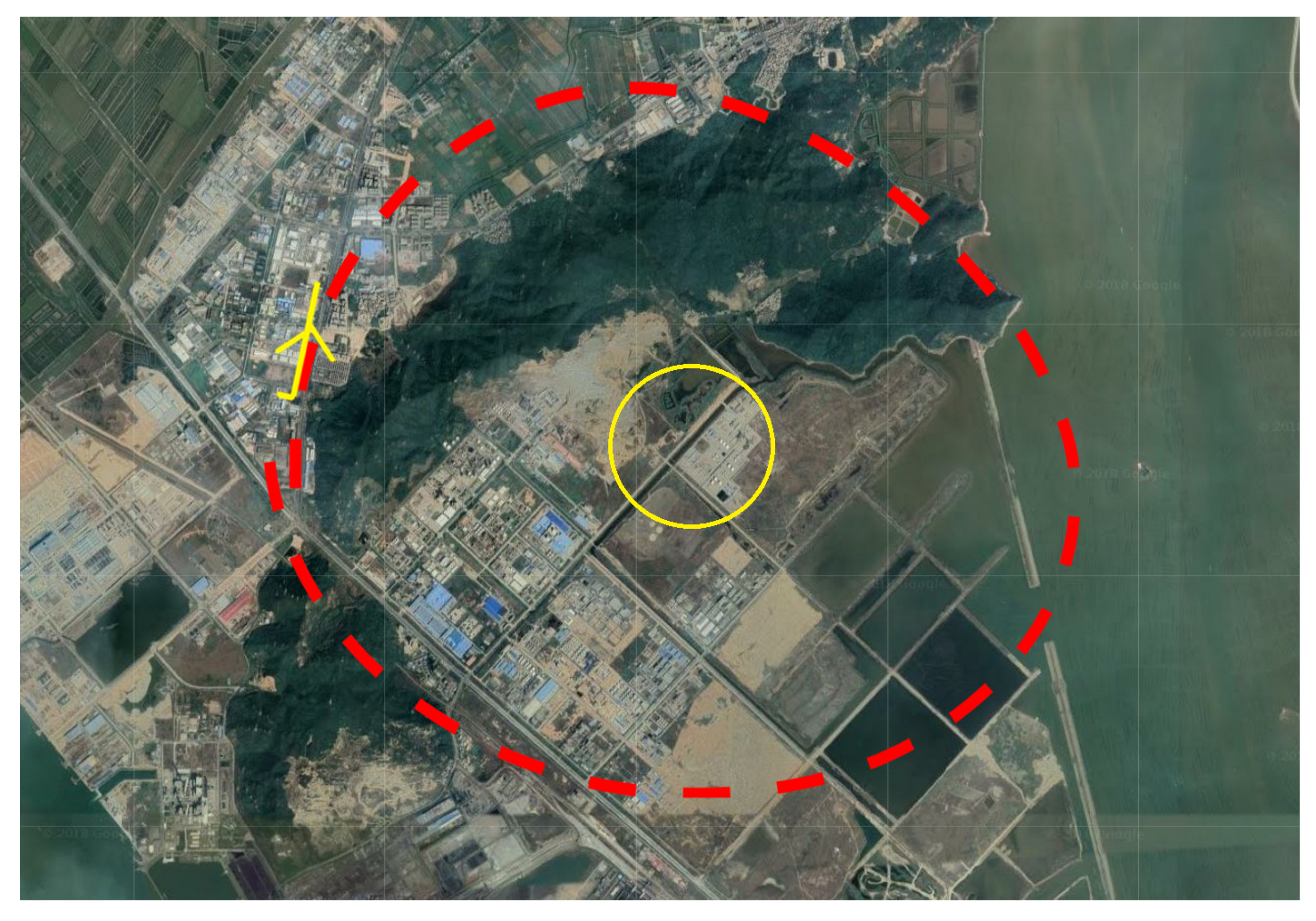
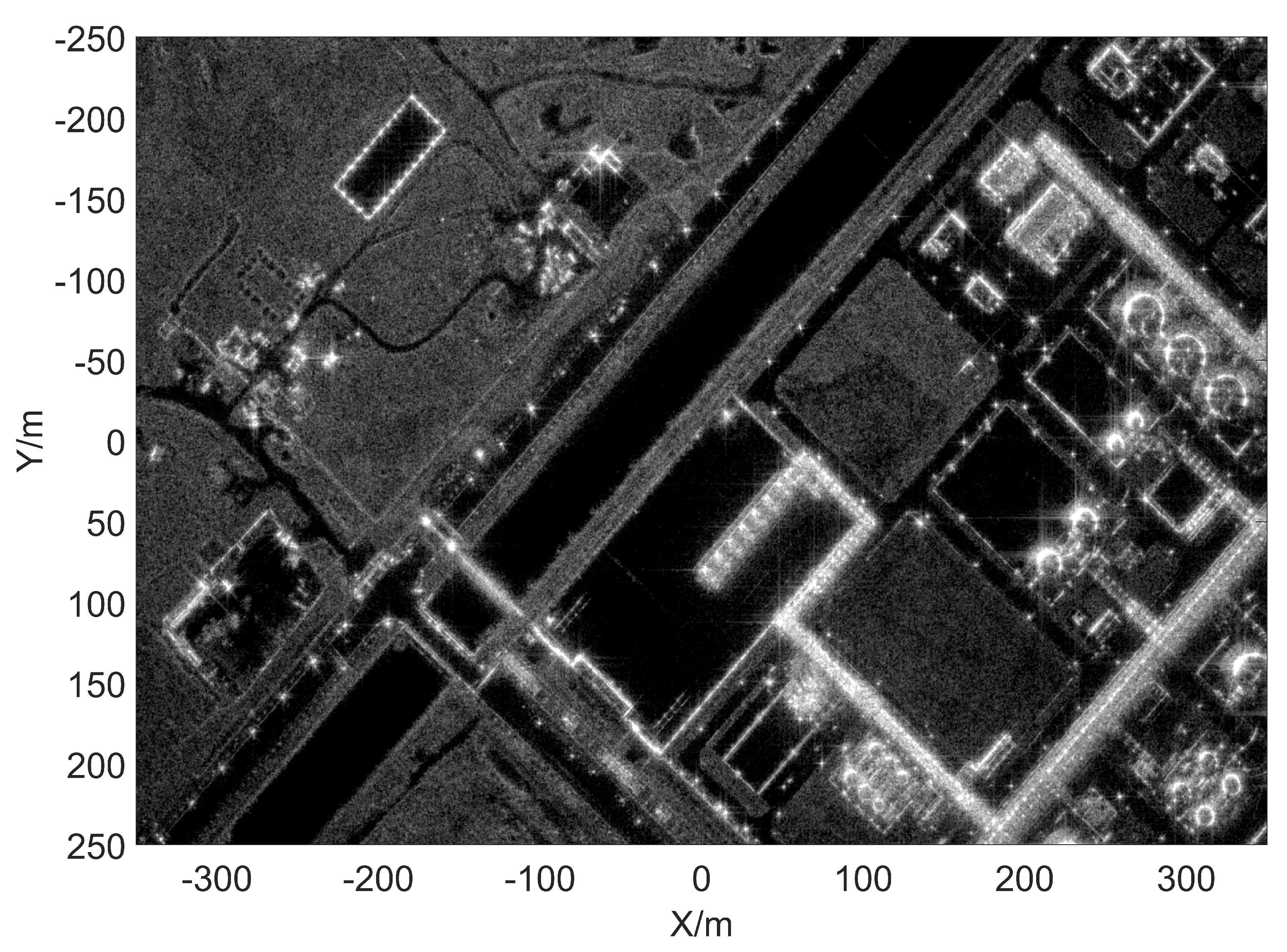
2. Datasets
3. The Multi-Angular Statistical Property Analysis
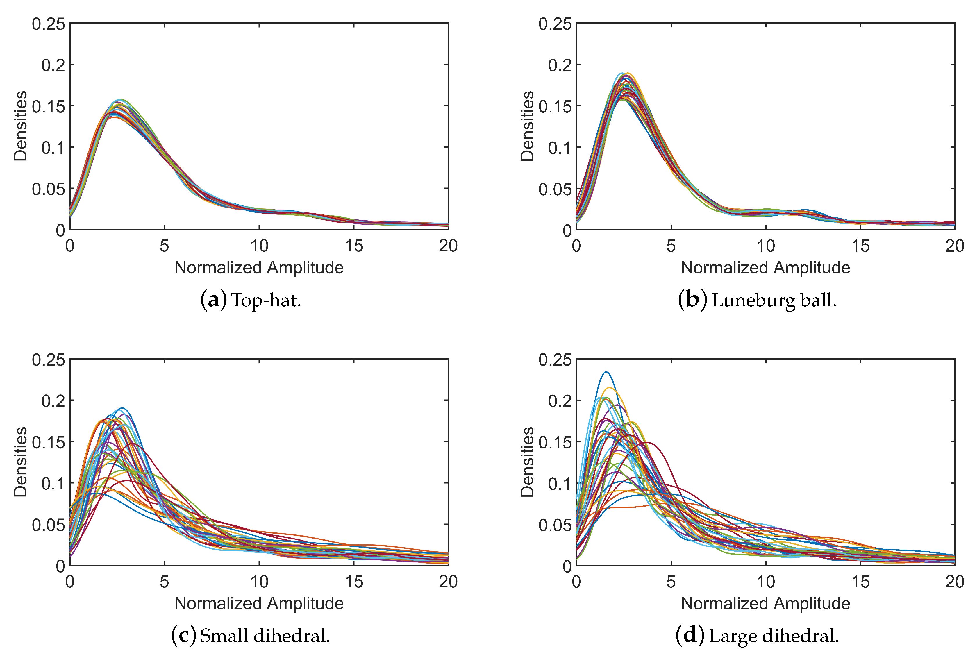
3.1. The Statistical Property of Anisotropic and Isotropic Scatterings
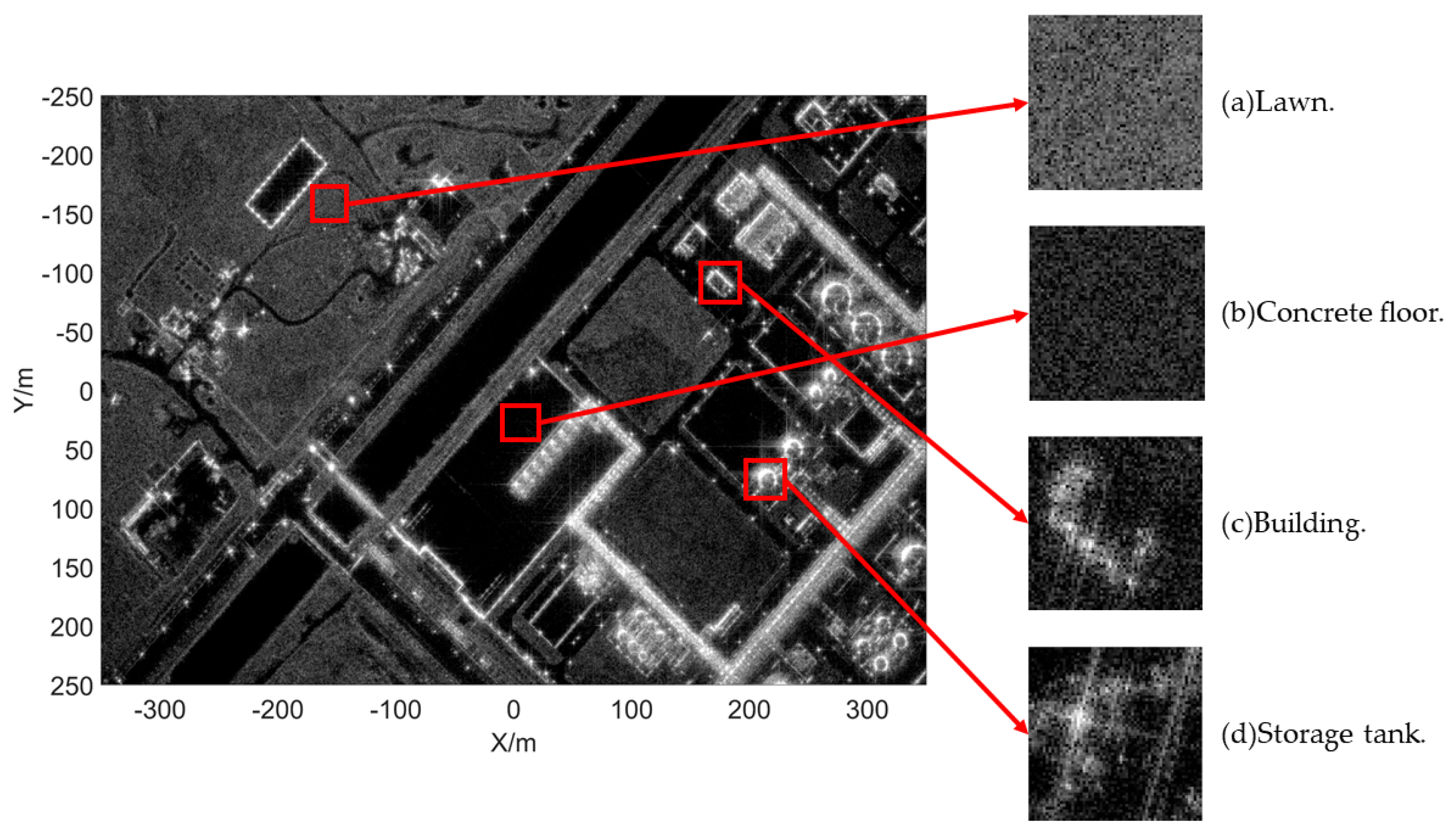
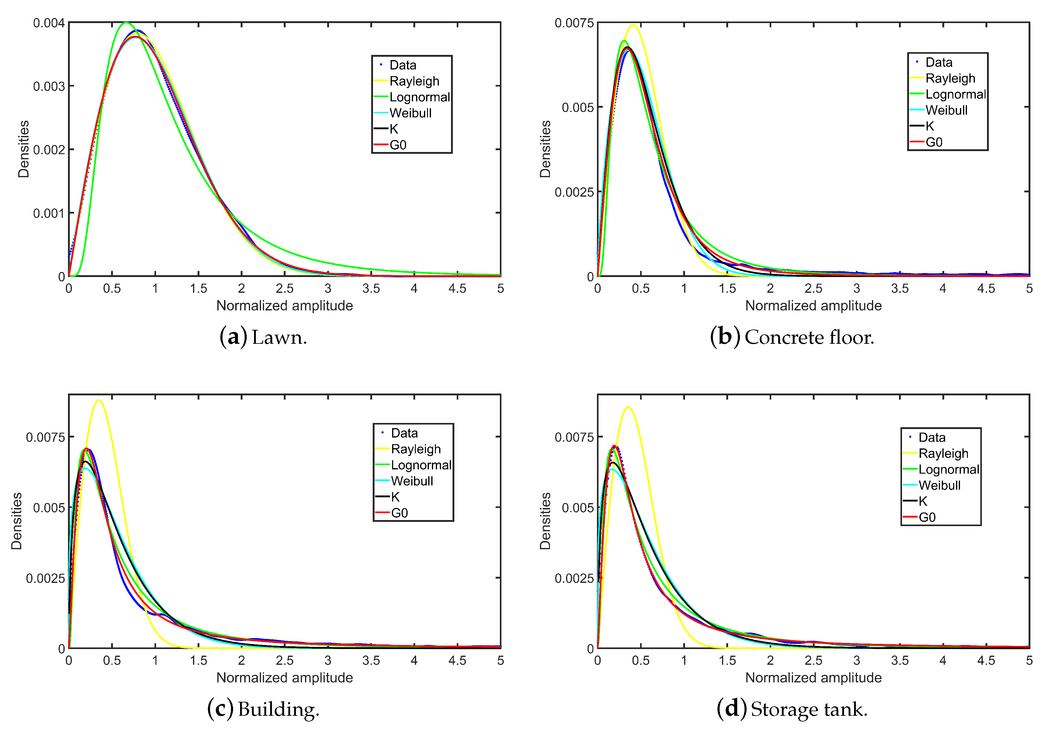
3.2. The Statistical Model of the High-Resolution Multi-Angular SAR Images
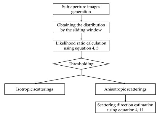
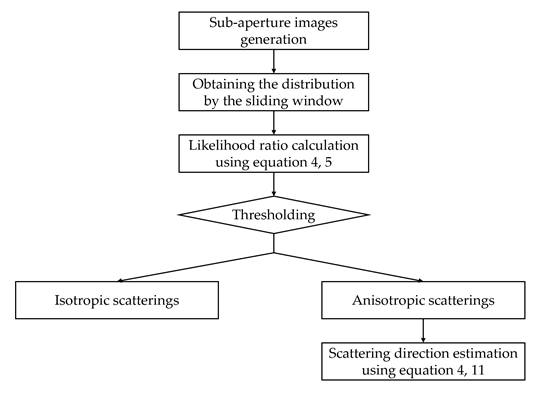
4. Methodology
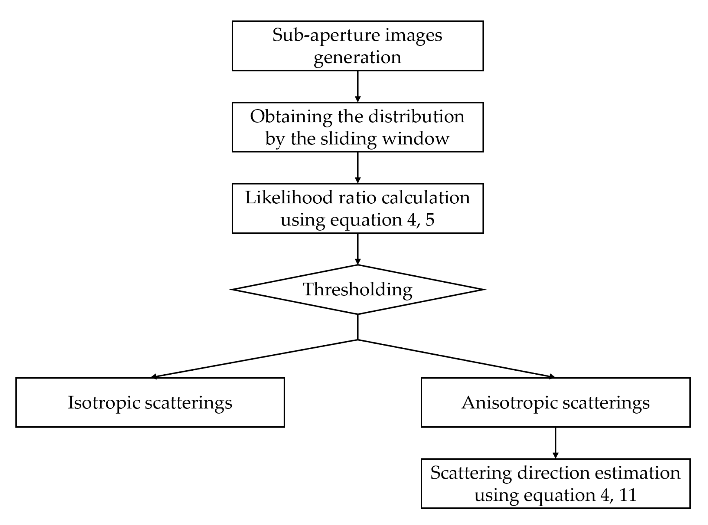
4.1. Anisotropic Scattering Analysis Method
4.2. Method Used for Comparison
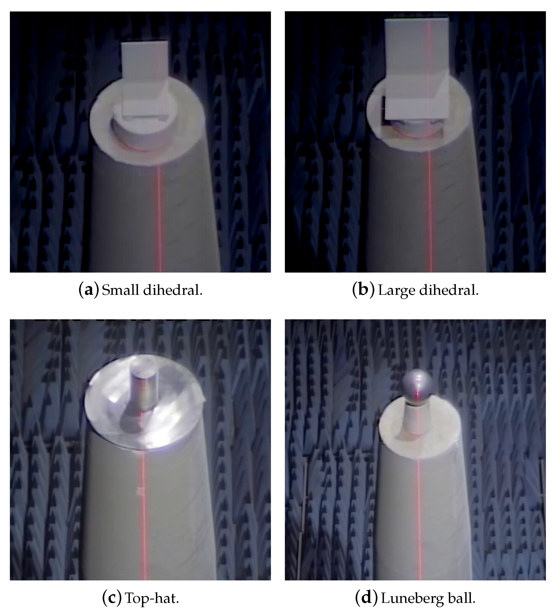
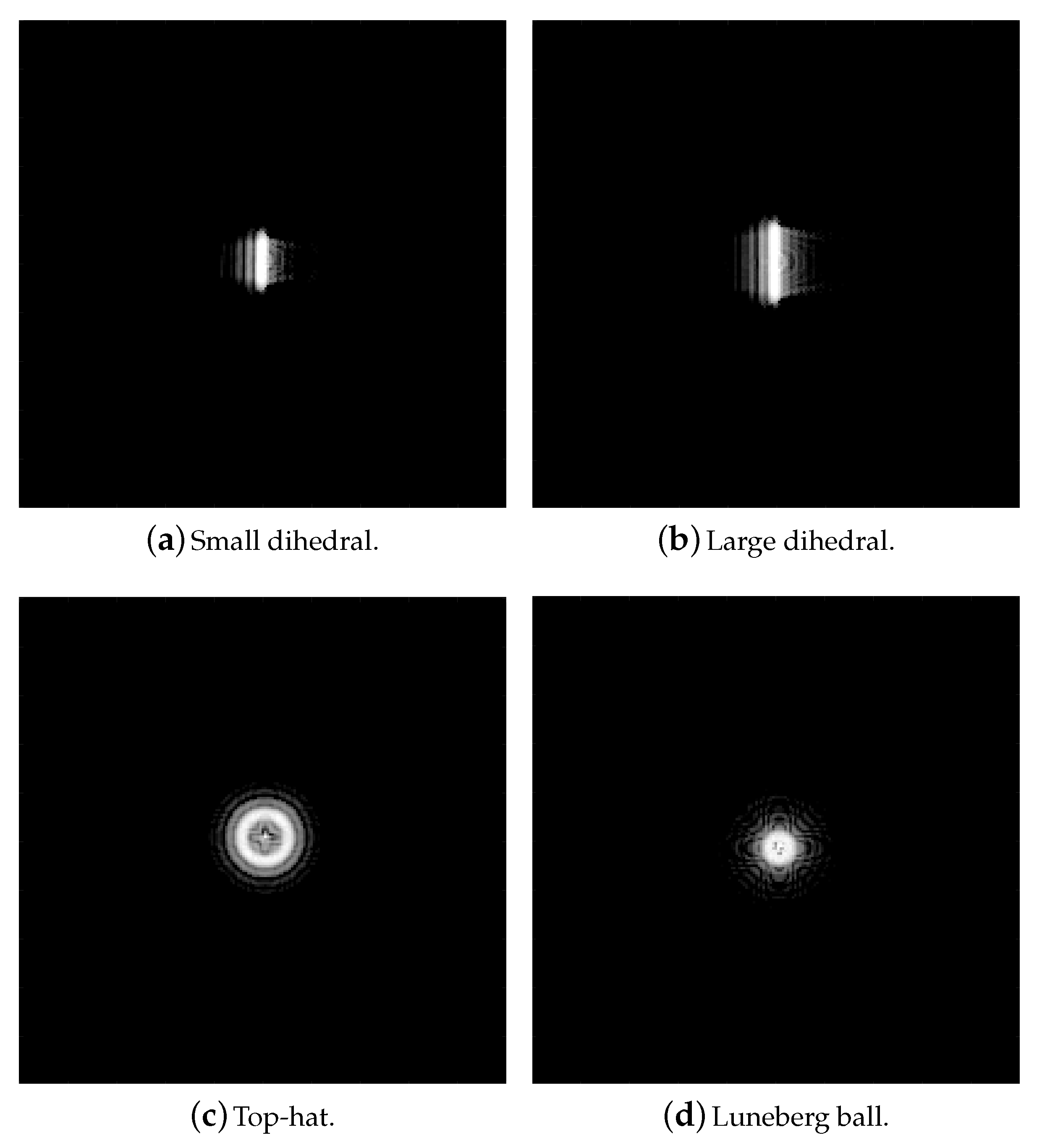
5. Experiment and Results
6. Discussion
7. Conclusions
Author Contributions
Funding
Conflicts of Interest
References
- Thompson, P.; Wahl, D.E.; Eichel, P.H.; Ghiglia, D.C.; Jakowatz, C.V.J. Spotlight-Mode Synthetic Aperture Radar: A Signal Processing Approach; Springer: Berlin/Heidelberg, Germany, 1996; Volume 26, pp. 330–332. [Google Scholar]
- Munson, D.C.; Visentin, R.L. A signal processing view of strip-mapping synthetic aperture radar. IEEE Trans. Acoust. Speech Signal Process. 1989, 37, 2131–2147. [Google Scholar] [CrossRef]
- Margarit, G.; Tabasco, A. Ship Classification in Single-Pol SAR Images Based on Fuzzy Logic. IEEE Trans. Geosci. Remote Sens. 2011, 49, 3129–3138. [Google Scholar] [CrossRef]
- Duquenoy, M.; Ovarlez, J.P.; Ferro-Famil, L.; Pottier, E.; Vignaud, L. Characterization of scatterers by their anisotropic and dispersive behavior. In Proceedings of the IEEE International Geoscience & Remote Sensing Symposium, Barcelona, Spain, 23–28 July 2007. [Google Scholar]
- Ferro-Famil, L.; Reigber, A.; Pottier, E.; Boerner, W.M. Scene characterization using subaperture polarimetric sar data. IEEE Trans. Geosci. Remote Sens. 2003, 41, 2264–2276. [Google Scholar] [CrossRef]
- Gherboudj, I.; Magagi, R.; Berg, A.A.; Toth, B. Soil moisture retrieval over agricultural fields from multi-polarized and multi-angular RADARSAT-2 SAR data. Remote Sens. Environ. 2011, 115, 33–43. [Google Scholar] [CrossRef]
- Schmitt, M.; Maksymiuk, O.; Magnard, C.; Stilla, U. Radargrammetric registration of airborne multi-aspect SAR data of urban areas. ISPRS J. Photogramm. Remote Sens. 2013, 86, 11–20. [Google Scholar] [CrossRef]
- Ash, J.; Ertin, E.; Potter, L.C.; Zelnio, E. Wide-Angle Synthetic Aperture Radar Imaging: Models and algorithms for anisotropic scattering. Signal Process. Mag. IEEE 2014, 31, 16–26. [Google Scholar] [CrossRef]
- Zhao, Y.; Hong, W.; Lin, Y.; Yu, L. Adaptive imaging of anisotropic target based on circular-SAR. Electron. Lett. 2016, 52, 1406–1408. [Google Scholar] [CrossRef]
- Yue, Z.; Yun, L.; Ping, W.Y.; Wen, H.; Yu, L. Target multi-aspect scattering sensitivity feature extraction based on Circular-SAR. In Proceedings of the IGARSS 2016—2016 IEEE International Geoscience and Remote Sensing Symposium, Beijing, China, 10–15 July 2016. [Google Scholar]
- Xue, F.; Lin, Y.; Hong, W.; Yin, Q.; Zhang, B.; Shen, W.; Zhao, Y. Analysis of Azimuthal Variations Using Multi-Aperture Polarimetric Entropy with Circular SAR Images. Remote Sens. 2018, 10, 123. [Google Scholar] [CrossRef] [Green Version]
- Li, Y.; Qiang, Y.; Yun, L.; Wen, H. Anisotropy Scattering Detection From Multiaspect Signatures of Circular Polarimetric SAR. IEEE Geosci. Remote Sens. Lett. 2018, 15, 1575–1579. [Google Scholar] [CrossRef]
- Barber, J. A Generalized Likelihood Ratio Test for Coherent Change Detection in Polarimetric SAR. IEEE Geosci. Remote Sens. Lett. 2015, 12, 1873–1877. [Google Scholar] [CrossRef]
- Krylov, V.A.; Moser, G.; Voisin, A.; Serpico, S.B.; Zerubia, J. Change detection with synthetic aperture radar images by Wilcoxon statistic likelihood ratio test. In Proceedings of the ICIP International Conference on Image Processing, Orlando, FL, USA, 30 September–3 October 2012. [Google Scholar]
- Xiong, B.; Chen, J.M.; Kuang, G. A change detection measure based on a likelihood ratio and statistical properties of SAR intensity images. Remote Sens. Lett. 2012, 3, 267–275. [Google Scholar] [CrossRef]
- Schneider, R.Z.; Papathanassiou, K.; Hajnsek, I.; Moreira, A. Polarimetric and interferometric characterization of coherent scatterers in urban areas. IEEE Trans. Geosci. Remote Sens. 2006, 44, 971–984. [Google Scholar] [CrossRef]
- D’Hondt, O.; Lopez-Martinez, C.; Ferro-Famil, L.; Pottier, E. Spatially Nonstationary Anisotropic Texture Analysis in SAR Images. IEEE Trans. Geosci. Remote Sens. 2008, 45, 3905–3918. [Google Scholar] [CrossRef]
- Xue, F.T.; Yang, L.; Yun, L.; Qiang, Y.; Wen, H. An improved detection and feature retrieval method of anisotropic scattering for multi-aspect PolSAR data processing based on DRIA framework. In Proceedings of the 2016 IEEE International Geoscience and Remote Sensing Symposium (IGARSS), Beijing, China, 10–15 July 2016. [Google Scholar]
- Cantalloube, H.; Koeniguer, E.C. Assessment of physical limitations of High Resolution on targets at X-band from Circular SAR experiments. In Proceedings of the 7th European Conference on Synthetic Aperture Radar, Friedrichshafen, Germany, 2–5 June 2008. [Google Scholar]
- Soumekh, M. Reconnaissance with slant plane circular SAR imaging. IEEE Trans. Image Process. A Publ. IEEE Signal Process. Soc. 1996, 5, 1252–1265. [Google Scholar] [CrossRef] [Green Version]
- Chan, T.K.; Kuga, Y.; Ishimaru, A. Experimental studies on circular SAR imaging in clutter using angular correlation function technique. Geosci. Remote Sens. IEEE Trans. 1999, 37, 2192–2197. [Google Scholar] [CrossRef]
- Yun, L.; Wen, H.; Tan, W.; Wang, Y.; Xiang, M. Airborne circular SAR imaging: Results at P-band. In Proceedings of the 2012 IEEE International Geoscience and Remote Sensing Symposium, Munich, Germany, 22–27 July 2012. [Google Scholar]
- Pinheiro, M.; Prats, P.; Scheiber, R.; Nannini, M.; Reigber, A. Tomographic 3D Reconstruction From Airborne Circular SAR. In Proceedings of the 2009 IEEE International Geoscience and Remote Sensing Symposium, IGARSS 2009, Cape Town, South Africa, 12–17 July 2009. [Google Scholar]
- Palm, S.; Oriot, H.M.; Cantalloube, H.M. Radargrammetric DEM Extraction Over Urban Area Using Circular SAR Imagery. IEEE Trans. Geosci. Remote Sens. 2012, 50, 4720–4725. [Google Scholar] [CrossRef]
- Knott, E.F. Radar Cross Section Measurements. Proc. IEEE 2005, 75, 498–516. [Google Scholar]
- Paladini, R.; Martorella, M.; Berizzi, F. Classification of Man-Made Targets via Invariant Coherency-Matrix Eigenvector Decomposition of Polarimetric SAR/ISAR Images. IEEE Trans. Geosci. Remote Sens. 2011, 49, 3022–3034. [Google Scholar] [CrossRef]
- Duquenoy, M.; Ovarlez, J.P.; Vignaud, L.; Ferro-Famil, L.; Pottier, E. Classification based on the polarimetric dispersive and anisotropic behavior of scatterers. In Proceedings of the International Workshop on Science & Applications of Sar Polarimetry & Polarimetric Interferometry, Frascati, Italy, 22–26 January 2007; Volume 644. [Google Scholar]
- Ulander, L.M.H.; Hellsten, H.; Stenstrom, G. Synthetic-aperture radar processing using fast factorized back-projection. IEEE Trans. Aerosp. Electron. Syst. 2003, 39, 760–776. [Google Scholar] [CrossRef] [Green Version]
- Ponce, O.; Prats, P.; Rodriguez-Cassola, M.; Scheiber, R.; Reigber, A. Processing Of Circular SAR Trajectories With Fast Factorized Back-Projection. In Proceedings of the IEEE International Geoscience and Remote Sensing Symposium (IGARSS), Vancouver, BC, Canada, 24–29 July 2011. [Google Scholar]
- Jakeman, E.; Pusey, P. A model for non-Rayleigh sea echo. Antennas Propag. IEEE Trans. 1976, 24, 806–814. [Google Scholar] [CrossRef]
- Jao, J. Amplitude distribution of composite terrain radar clutter and the K-Distribution. IEEE Trans. Antennas Propag. 1984, 32, 1049–1062. [Google Scholar]
- Lee, J.S.; Hoppel, K.; Mango, S.; Miller, A. Intensity and phase statistics of multilook polarimetric and interferometric SAR imagery. IEEE Trans. Geosci. Remote Sens. 1994, 32, 1017–1028. [Google Scholar]
- Ulaby, F.T. Textural information in SAR images. IEEE Trans. Geosci. Remote Sens. 1986, 24, 235–245. [Google Scholar] [CrossRef]
- Magee, L. R2 Measures Based on Wald and Likelihood Ratio Joint Significance Tests. Am. Stat. 1990, 44, 250–253. [Google Scholar]
- Willmott, C.; Matsuura, K. Advantages of the mean absolute error (MAE) over the root mean square error (RMSE) in assessing average model performance. Clim. Res. 2005, 30, 79–82. [Google Scholar] [CrossRef]
- Mittlböck, M.; Waldhör, T. Adjustments for R2-measures for Poisson regression models. Comput. Stat. Data Anal. 2000, 34, 461–472. [Google Scholar] [CrossRef]
- Kuruoglu, E.E.; Zerubia, J. Modeling SAR Images With a Generalization of the Rayleigh Distribution. IEEE Trans. Image Process. 2004, 13, 527–533. [Google Scholar] [CrossRef]
- Szajnowski, W.J. Estimators of Log-Normal Distribution Parameters. IEEE Trans. Aerosp. Electron. Syst. 1977, AES-13, 533–536. [Google Scholar] [CrossRef]
- Fernandes, D. Segmentation of SAR images with Weibull distribution. In Proceedings of the 1998 IEEE International Geoscience and Remote Sensing Symposium Proceedings, Seattle, WA, USA, 6–10 July 1998. [Google Scholar]
- Wang, H.; Ouchi, K. Accuracy of the K-Distribution Regression Model for Forest Biomass Estimation by High-Resolution Polarimetric SAR: Comparison of Model Estimation and Field Data. IEEE Trans. Geosci. Remote Sens. 2008, 46, 1058–1064. [Google Scholar] [CrossRef]
- MLAFrery, A.C.; Muller, H.J. A model for extremely heterogeneous clutter. IEEE Trans. Geosci. Remote Sens. 1997, 35, 648–659. [Google Scholar]
- Gambini, J.; Mejail, M.E.; Jacobo-Berlles, J.; Frery, A.C. Accuracy of edge detection methods with local information in speckled imagery. Stat. Comput. 2008, 18, 15–26. [Google Scholar] [CrossRef]
- Vasconcellos, K.L.P.; Frery, A.C.; Silva, L.B. Improving estimation in speckled imagery. Comput. Stat. 2005, 20, 503–519. [Google Scholar] [CrossRef] [Green Version]
- Freitas, C.C.; Frery, A.C.; Correia, A.H. The polarimetric G distribution for SAR data analysis. Environmetrics 2005, 16, 13–31. [Google Scholar] [CrossRef]
- Feng, S.; Lin, Y.; Wang, Y.; Yang, Y.; Shen, W.; Teng, F.; Hong, W. DEM Generation With a Scale Factor Using Multi-Aspect SAR Imagery Applying Radargrammetry. Remote Sens. 2020, 12, 556. [Google Scholar] [CrossRef] [Green Version]


| Parameter | Description |
|---|---|
| Carrier frequency | 15 GHz |
| Bandwidth | 600 MHz |
| Azimuthal sampling interval | |
| Look-down angle |
| Parameter | Description |
|---|---|
| Carrier frequency | 5.4 GHz |
| Bandwidth | 560 MHz |
| PRF | 2358 Hz |
| Look-down angle | |
| Flight height | 3 km |
| Flight Radius | 5 km |
| Adjusted R-Square | Lawn | Concrete Floor | Building | Storage Tank |
|---|---|---|---|---|
| Rayleigh | 0.9977 | 0.9542 | 0.7120 | 0.8305 |
| Lognormal | 0.9732 | 0.9767 | 0.9758 | 0.9857 |
| Weibull | 0.9983 | 0.9793 | 0.9314 | 0.9655 |
| K | 0.9989 | 0.9835 | 0.9501 | 0.9792 |
| G | 0.9989 | 0.9907 | 0.9908 | 0.9959 |
| RMSE | Lawn | Concrete Floor | Building | Storage Tank |
|---|---|---|---|---|
| Rayleigh | 0.0100 | 0.0766 | 0.1364 | 0.0971 |
| Lognormal | 0.0344 | 0.0528 | 0.0395 | 0.0282 |
| Weibull | 0.0087 | 0.0547 | 0.0665 | 0.0439 |
| K | 0.0070 | 0.0460 | 0.0567 | 0.0340 |
| G | 0.0070 | 0.0345 | 0.0244 | 0.0150 |
© 2020 by the authors. Licensee MDPI, Basel, Switzerland. This article is an open access article distributed under the terms and conditions of the Creative Commons Attribution (CC BY) license (http://creativecommons.org/licenses/by/4.0/).
Share and Cite
Teng, F.; Lin, Y.; Wang, Y.; Shen, W.; Feng, S.; Hong, W. An Anisotropic Scattering Analysis Method Based on the Statistical Properties of Multi-Angular SAR Images. Remote Sens. 2020, 12, 2152. https://0-doi-org.brum.beds.ac.uk/10.3390/rs12132152
Teng F, Lin Y, Wang Y, Shen W, Feng S, Hong W. An Anisotropic Scattering Analysis Method Based on the Statistical Properties of Multi-Angular SAR Images. Remote Sensing. 2020; 12(13):2152. https://0-doi-org.brum.beds.ac.uk/10.3390/rs12132152
Chicago/Turabian StyleTeng, Fei, Yun Lin, Yanping Wang, Wenjie Shen, Shanshan Feng, and Wen Hong. 2020. "An Anisotropic Scattering Analysis Method Based on the Statistical Properties of Multi-Angular SAR Images" Remote Sensing 12, no. 13: 2152. https://0-doi-org.brum.beds.ac.uk/10.3390/rs12132152