Article

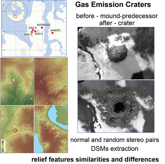
Gas Emission Craters and Mound-Predecessors in the North of West Siberia, Similarities and Differences

1
Cryolithology and Glaciology Department, Faculty of Geography, Lomonosov Moscow State University, 119991 Moscow, Russia
2
Earth Cryosphere Institute Tyumen Scientific Centre SB RAS, 625000 Tyumen, Russia
3
Cartography and Geoinformatics Department, Faculty of Geography, Lomonosov Moscow State University, 119991 Moscow, Russia
4
SCANEX Group, 121059 Moscow, Russia
5
OpenWeatherMap, Inc., Lake Success, NY 11042, USA
6
Agrarian-Technological Institute, Peoples’ Friendship University of Russia, 117198 Moscow, Russia
7
TOTAL S.A., CSTJF, 64018 Pau CEDEX, France
8
Russian Center for Arctic Development, 629007 Salekhard, Russia
9
TOTAL S.A., Place Jean Millier, 92078 Paris La Défense CEDEX, France
*
Author to whom correspondence should be addressed.
Remote Sens. 2020, 12(14), 2182; https://0-doi-org.brum.beds.ac.uk/10.3390/rs12142182
Submission received: 26 May 2020 / Revised: 28 June 2020 / Accepted: 6 July 2020 / Published: 8 July 2020
(This article belongs to the Section Remote Sensing in Geology, Geomorphology and Hydrology)

Abstract

:
Detailed analysis of five gas emission craters (GEC) found in the north of West Siberia is presented. Remote sensing data used in the study is verified by field surveys. Previous studies show that all of the GECs were preceded by mounds 2 to 6 m high and 20 to 55 m in diameter. GECs initially were 20–25 m in diameter, which increased in the first years of their existence. GECs are found in various environmental (shrublands or moss-grass tundra) and geomorphic (river valley, terrace, slopes) conditions. The objective of the paper is to identify common and differing geomorphologic and environmental characteristics of all the five GEC, and their mound-predecessors. The study is based on a compilation of DSMs before and after the GEC formation using very high-resolution satellite imagery stereo pairs compared to ArcticDEM project data. Diversity of terrain and environmental settings along with rather a narrow range of GEC and mound-predecessor morphometric parameters allows concluding that the mechanism of GEC formation is most likely similar for all the GEC and is controlled rather by internal geologic and cryolithologic structure than by any surface properties.

Graphical Abstract

1. Introduction

Gas emission craters (GECs) comprise a recently observed phenomenon in the permafrost zone. The first known GEC was discovered in the central part of the Yamal Peninsula in the summer of 2014. This discovery prompted studies of this feature and a search for similar craters. Information from local residents helped to discover other GECs. As of now, just a few features of this kind have been surveyed in the northern part of West Siberia (Figure 1). Although some researchers also depict other GECs [1,2], there are no published findings from comprehensive operations similar to those carried out on GECs shown in Figure 1. For that reason, other GECs will not be considered in this paper.
Initially we obtained information on the GECs position from field and helicopter observations. We compiled multi-temporal digital surface models (DSM) for an area around each GEC to reveal changes in the relief caused by mound and GEC formation. We established earlier that GEC-1 and AntGEC were preceded by mounds of various height [3,4,5]. These two GECs appeared to differ substantially in terms of their geomorphic position. AntGEC is located on the edge of a terrace; GEC-1 is located at the foot of a gentle slope.
Data on the morphometric properties of GEC-2 and GEC-3 have not been published thus far. Publications [1,6] only provided fragments of satellite images showing the state of the area before and after several GECs formation. Bogoyavlensky et al. [7] analyzed SeYkhGEC development by reviewing the event itself, and the resulting landforms, as well as remote sensing data before and after SeYkhGEC formation.
Due to a limited number of GECs, statistical analysis of GEC morphometry is not appropriate, yet an overview can be applied along with a qualitative/semi-quantitative classification of the environment in known GEC locations, including relief and microrelief, vegetation, hydrology, cryolithology, cryogenic processes, and landforms. Similar studies were performed by Khilimonyuk et al. [8] and Buldovicz et al. [9]. However, only a single GEC-1 was under study and those findings cannot be extrapolated to GECs located in other environmental and geomorphic conditions.
Special attention is paid to quantitative analysis of morphometric properties of mound-predecessors and GECs occurring in their place. Such an analysis can be done by processing satellite imagery and requires no field observations that are no longer possible once GECs had formed and flooded in a year. Accordingly, such analysis can provide the basis for identifying mounds with a similar nature and successive growth.
The objective of this study is to identify the common and differing geomorphic and environmental features of all GECs surveyed. We looked at (1) terrain features in GEC locations, (2) environmental surroundings of GECs, (3) morphometric parameters of mound-predecessors, (4) morphometric parameters of successive GECs, and (5) terrain changes caused by GEC formation.
Morphometric analysis is based on results from the processing of multi-temporal remote sensing satellite data and derivatives of the latter, as well as the field survey. Field survey has provided data on morphometric parameters of the terrain in key locations, their landscape, and geobotanic structure. Furthermore, the pattern of scattering of material ejected out of GEC was identified as supplemental information on the expelling force. It can be assumed that varying parameters are of little relevance for GEC formation, while common parameters can be considered as probable controls of GEC formation.
Considering the unavailability of actual detailed topographic maps, local DSM covering study sites are needed to access the current changes in relief. Depending on the size of the studied landforms (in plan and height), the necessary and sufficient detail level of such DSMs is selected. Taking into account the tasks of a retrospective analysis of changes in the relief with dimensions of a few meters in height and the higher availability of optical satellite imagery data with a sub-meter resolution, we selected these materials as a source for DSM extraction. We tried to get the most detailed models performing the data processing, and as a result, DSMs with a high node density of 1 m were obtained.
We have sampled and analyzed remote sensing data for four GECs in the Yamal Peninsula and 1 GEC in the Gydan Peninsula (Figure 1). Additionally, field data of various thoroughness were obtained for GEC-1, GEC-2, and GEC-3 in Yamal and AntGEC in Gydan. We did not visit SeYkhGEC infield, but it is necessary to include it in our research as an object with a similar mechanism, but the contrast in geomorphic position as it is located in the riverbed. For this GEC, we did not create a DSM but only used the ArcticDEM data [10] and multi-temporal satellite imagery. We also relied on published findings from a field survey of SeYkhGEC [7,11].

2. Study Area, Materials, and Methods

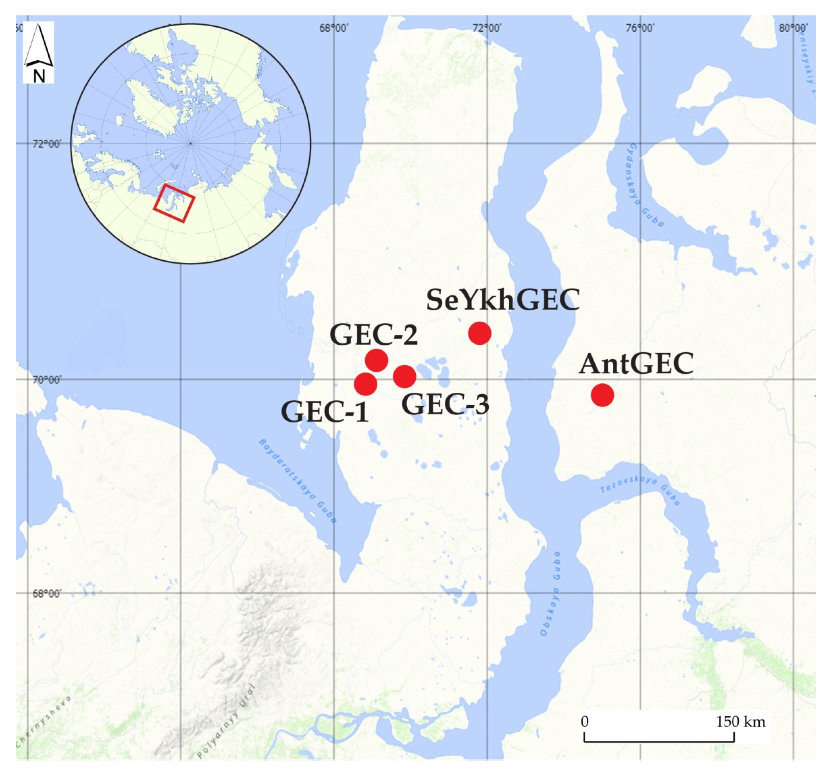
2.1. An Overview of the Study Area

All known GECs are located in the northern part of West-Siberian Lowland. This region is characterized by continuous permafrost with rather low ground temperature (−4 to −7 °C on average) [12], thick layers of tabular ground ice in the geological section, and methane in the form of both gas and gas clathrates in the upper 120 m of the section [13,14,15]. The relief in the study area consists of several geomorphic units including a floodplain 0–5 m high, and a series of fluvial-lacustrine-marine plains and terraces within the height interval of 7–85 m, dissected by rivers, lakes, drained lake basins (khasyreys), and thermoerosion ravines and gullies. High-centered sand polygons and polygonal peat plateaus often occupy flat hilltops of the plains, otherwise represented by hummocky tundra landscapes. High willow shrub thickets mainly cover concave slopes while dwarf birch shrubs dominate convex slopes.
Immediate surroundings of the GECs under study represented by a square 25 km2 in area have been identified as key sites. For these areas, stereo pairs of very-high resolution satellite imagery were ordered, DSMs created, and fieldwork carried out. There are certain differences in the geomorphic structure of key sites, identified by the analysis of field data and DSM interpretation.

2.2. Field Survey

Field studies have provided data on environmental characteristics of GEC locations (key sites), their cryolithology, and more [16,17,18,19]. The range of methods included photo documentation and sampling of ground ice and enclosing deposits, with a description of the surrounding landscape structure and occurrences of relief-forming cryogenic processes. Thematic interpretation of remote sensing data was carried out in the field as well. Several repetitive measurements of GEC rim and wall retreat due to the thaw and collapse of icy sediments were performed. The spatial position of frozen blocks ejected during GEC formation was identified during fieldwork as well. Findings from a field survey of SeYkhGEC and GEC-2 photographs taken from a helicopter in 2012 [20] were used to interpret the cryolithologic structure of ejected blocks and to confirm the presence of in-situ ice in walls of these GECs.

2.3. Remote Sensing Data Processing

To obtain morphometric properties of key sites and to identify changes in terrain associated with GEC formation, multi-temporal DSMs characterizing surface conditions before and after crater formation have been plotted and analyzed. An alternative is the analysis of the publicly available ArcticDEM circumpolar product [21]. Contemporary studies of Arctic regions rely extensively on ArcticDEM data for analyses of surface changes and morphometry of landforms. The Discussion below assesses the applicability of these data [10] to resolve tasks set in this study. Paper use the following ArcticDEM Stripes [10]: 1) based on images dated 19 April 2016 for SeYkhGEC, 2) based on images dated 09 June 2013 for GEC-1, 3) based on images dated 16 June 2016 for GEC-2.
A common issue for all key sites is poor availability of very-high-resolution (<1 m) images, especially stereo pairs. Thus, an important part of the research included approbation of a methodology for DSM extraction out of stereo pairs, obtained by different sensing systems as well as multi-temporal acquisitions (random stereo pairs).
We had chosen the semi-global matching (SGM) method for DSM extraction from stereo image data, based on past studies where stereo pairs compiled from multi-temporal images were processed [22,23]. SGM was first proposed by Hirshmuller with a detailed exposition in a 2005 paper [24] and subsequently refined [25,26]. Due to the metrics that are used, and innovative proximity computation techniques, this method yields dense points cloud extraction, even when multi-temporal images are taken at different illumination, spatial resolution, and low base to height ratio.
Remote data processing comprised a succession of the following stages:
  • Selecting satellite imagery closest to the determined time interval of the study GECs formation.
  • Photogrammetric processing of stereo pairs and DSM extraction.
  • DSM analysis, including computing the amount of ejected material and identifying changes in terrain.

2.3.1. Selecting Stereo Pairs of Satellite Images for DSM Extraction

At the first stage, we determined the date of formation for the GECs with known coordinates. To perform this task, we used available satellite imagery (Table 1). Formation dates of AntGEC and SeYkhGEC only were reported by observers (local residents).
At the next stage, we searched for very-high resolution images based on the established time of GEC formation and implemented them to compose stereo pairs and DSM. Stereo pairs were supplemented by available scenes (Table 2): (a) normal stereo pairs, (b) individual scenes from different orbits, including images from different satellites. The above-mentioned method was tested for the GEC-2 key site by composing a stereo pair from images taken by different camera systems over a multi-year timeframe (GeoEye-1 on 30 July 2010, and WorldView-2 on 11 September 2011), while the stereo pair for GEC-3 was composed of images acquired by a single WorldView-1 system but on different dates (5 June and 9 June 2011).

2.3.2. Photogrammetric Processing of Satellite Imagery

Compiled stereo pairs underwent photogrammetric processing with the ScanEx IMAGE Processor software package using a method described earlier [4]. The following sequence of operations was carried out: (1) alignment of images with each other using third-order rational polynomial coefficients (RPC); (2) automatic tie point measurement; (3) generation of a normalized stereo pair (transforming images into an epipolar plane); (4) generation of DSMs automatically; (5) post-processing of the resulting DSMs, filling over voids and artifacts, resulting from incorrect parallax computation in occlusions during automated stereo matching; (6) transformation of the resulting models into orthographic projection; (7) orthorectification of the left and right stereo images.
After the aggregated stereo image pairs were processed (Table 2), DSMs were created with a 1-m resolution in the Universal Transverse Mercator (UTM) projection with orthometric heights relative to the EGM2008 geoid.
The relative precision of DSM in terms of height was assessed using a method described and tested earlier [5]. This estimate is based on satellite orientation and scanning and relies on automated stereo matching methods providing sub-pixel precision (penultimate column in Table 2).
Tundra vegetation is mainly presented by grass and low shrub communities with height not exceeding 0.5 m above the surface. This height is within DSM relative height accuracy. Therefore, we exclude vegetation cover from the analysis of DSM as a possible reason for the relief change. All changes in DSM between various time slices we consider as changes in relief.
Source satellite imagery was subjected to orthorectification based on DSMs compiled in this study. We used the orthorectification algorithm of Sonyushkin [27], which preserves photometric properties of source images, a crucial factor for automated thematic interpretation. Due to detailed DSMs (1-m resolution), the quality of resulting orthophotomaps allows us to compare them at the pixel level.

2.3.3. Computations from DSM

Considering that relative height accuracy values are close enough (mainly between 0.35 and 0.55 m) for all multi-temporal DSMs (Table 2), a comparison can be performed across key sites. Changes in relief were computed as a difference between DSMs before and after GEC formation. When performing the analysis of the DSM difference, the confidence level was introduced. The confidence level values for each DSM pair was calculated as the square root of the sum of the squared accuracy of each DSM in pair since the accuracy values obtained can be considered independent values (Table 2, last column). Thus, relief changes not exceeding this level were excluded.
The slope value of the surface surrounding mound-predecessors was calculated using the average maximum technique [28]. Mound-predecessor location steepness was characterized by slope angle values from the nearest pixels around mound foot. A range of values was listed in case the slope angle varied in the vicinity of the mound.

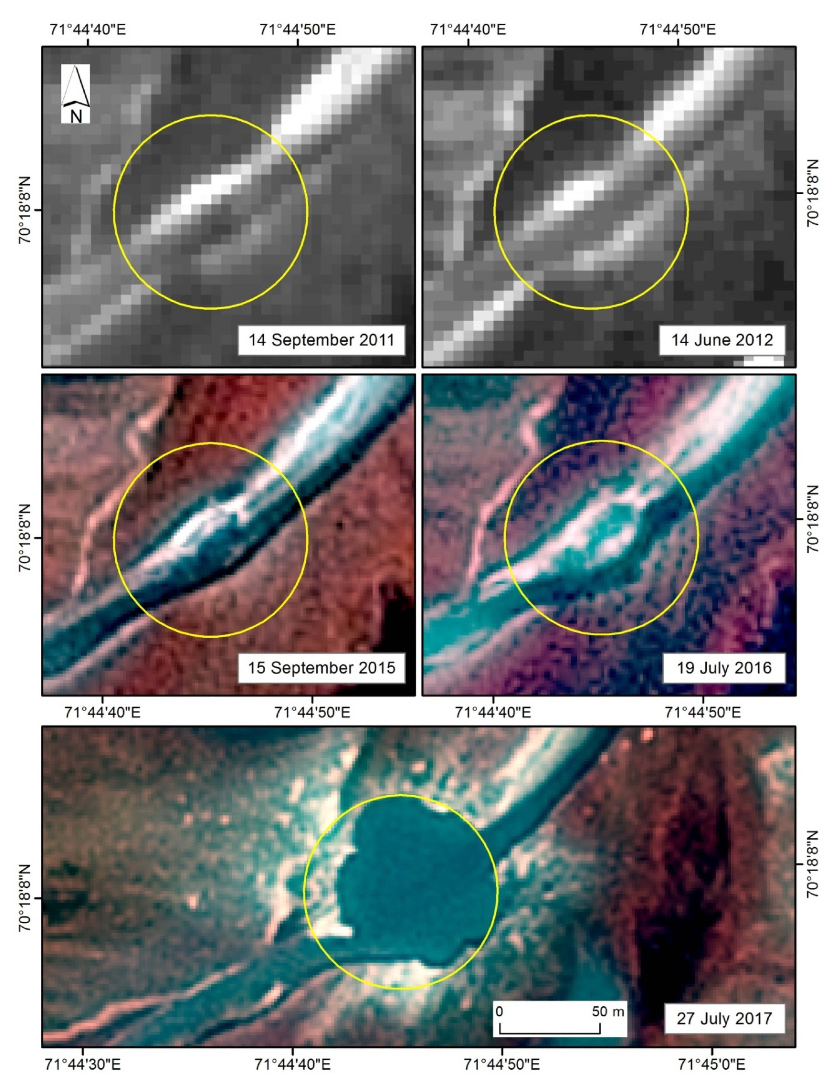
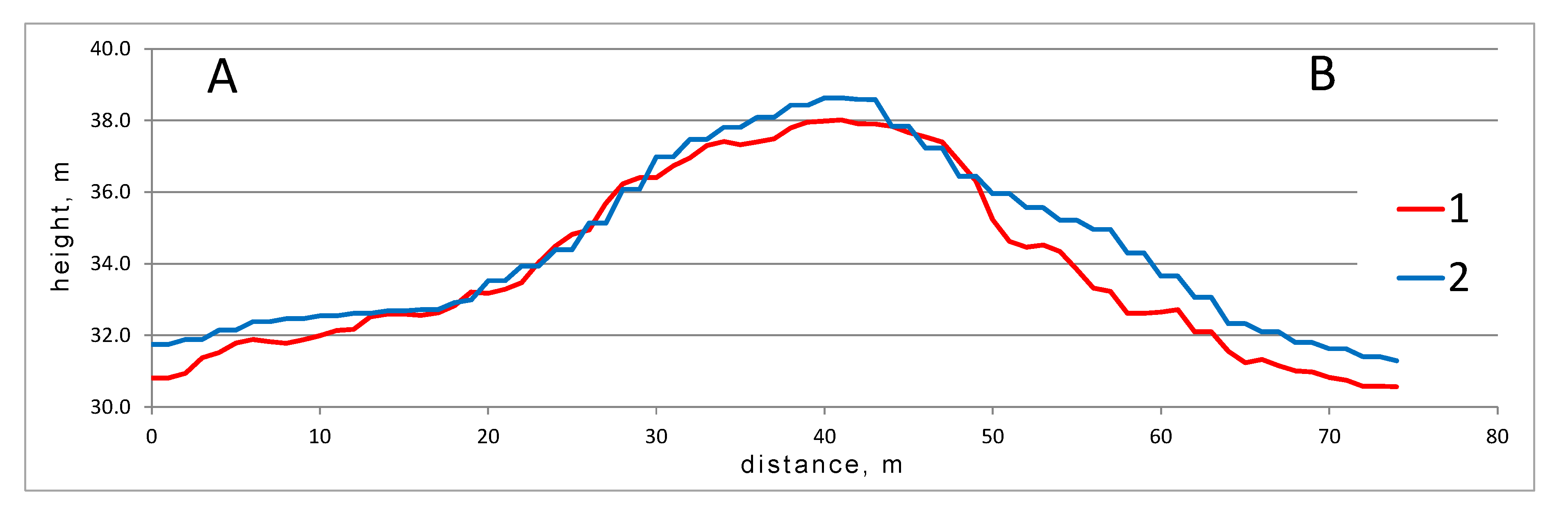
2.3.4. Analyzing Dynamics of the SeYkhGEC Mound-Predecessor Growth

The SeYkhGEC mound-predecessor formed in such a short time (three–four years) that its growth fits entirely into a time interval for which high-resolution images are available. Landforms from multi-temporal imagery were interpreted to identify the dynamics of mound-predecessor growth. A historical analysis of SPOT5 imagery from 2011 and 2012 and SPOT7 imagery from 2015, 2016, and 2017, allowed us to identify clearly observable lateral riverbed deformation in the location of mound-predecessor. The dimensions of the resulting mound and its growth dynamics are calculated using riverbed deformation values.

3. Results

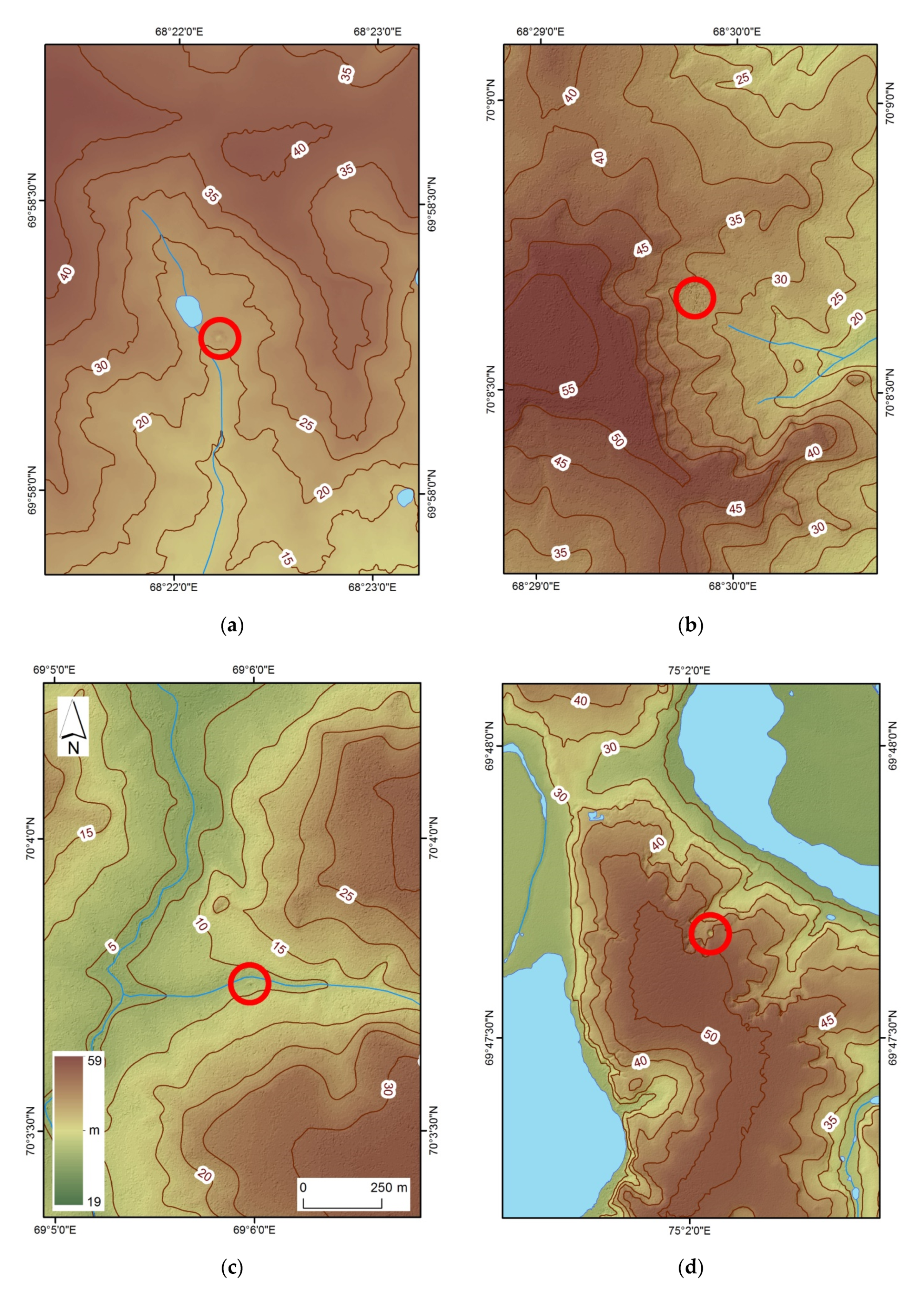
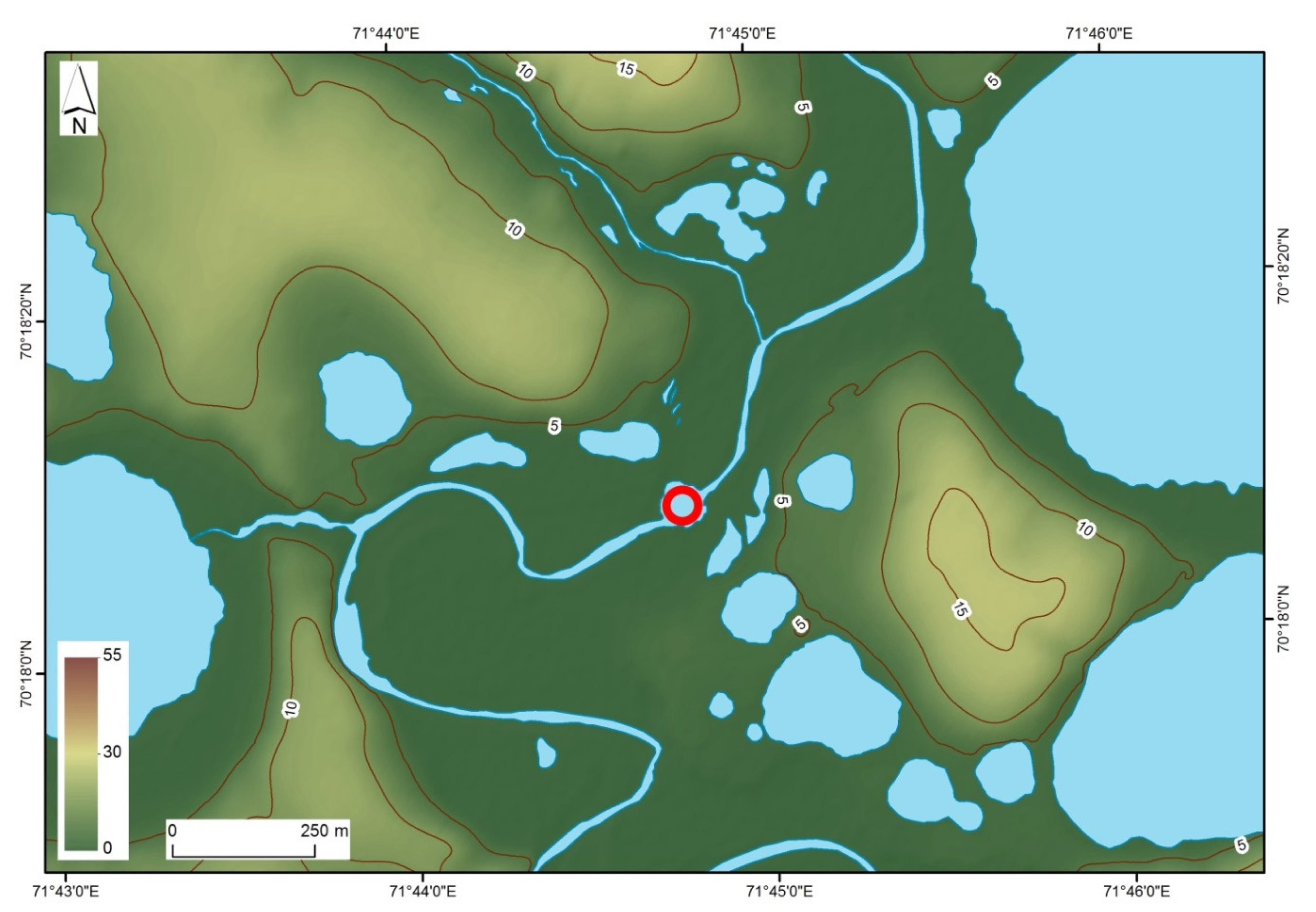
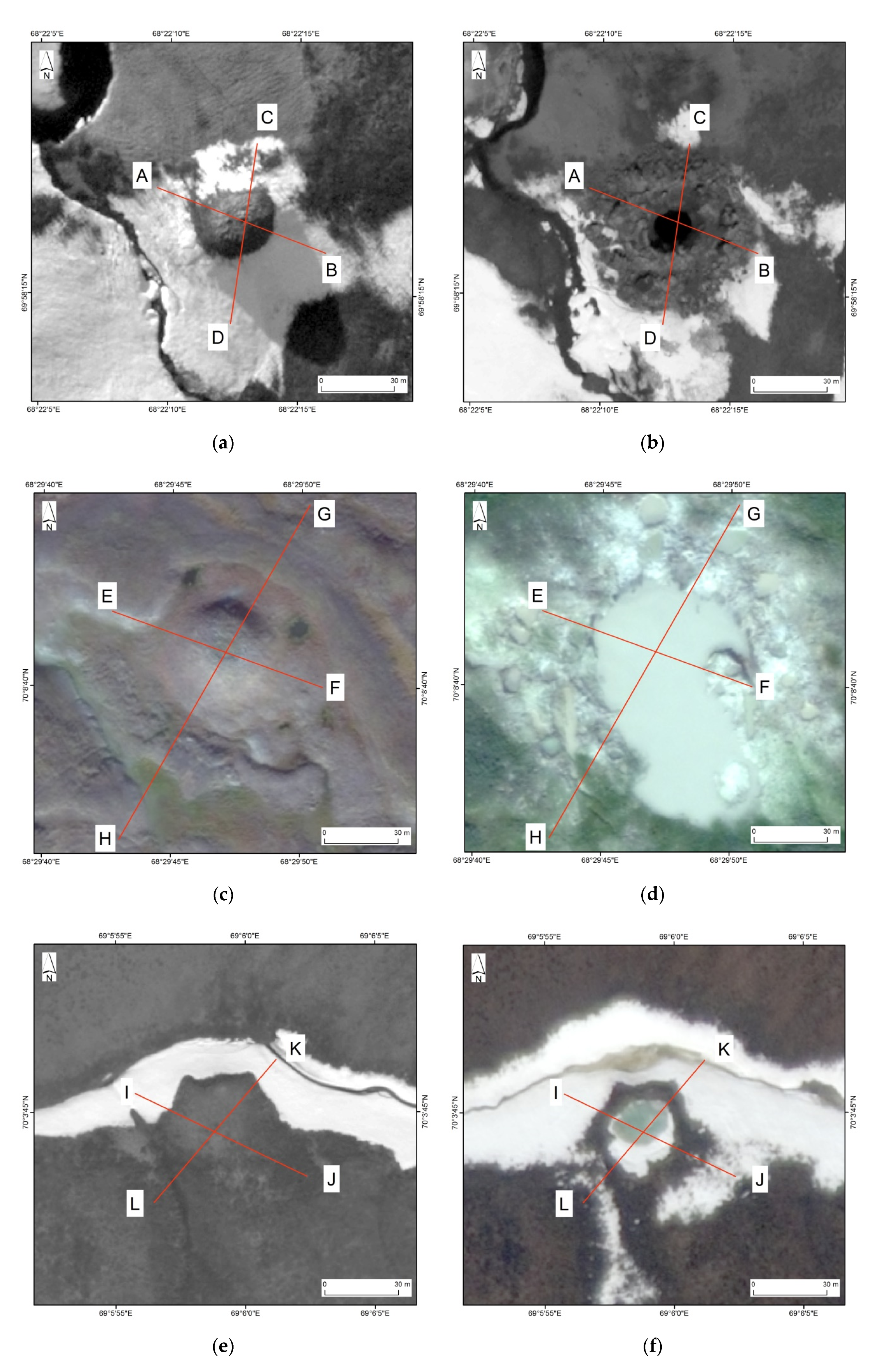
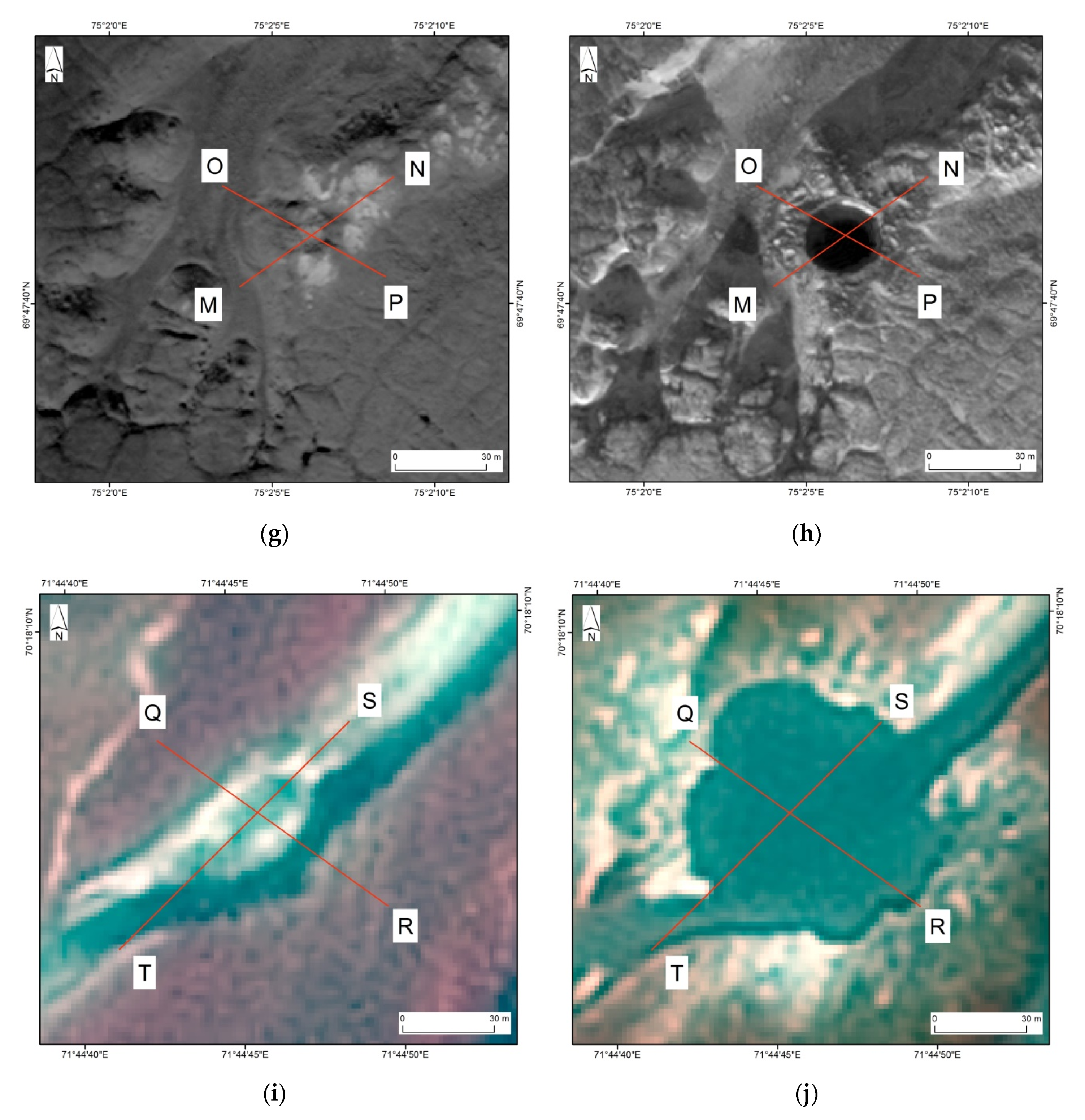
3.1. Geomorphic and Environmental Characteristics of Gas Emission Crater Key Sites

Analysis of available field data on environmental and geocryological settings of key sites, together with the respective DSMs, allowed to identify both similarities and significant dissimilarities in the geomorphic properties of GECs location. The characteristics detailed below encompass each key site as a whole, while Figure 2 only shows fragments immediately adjacent to the GEC.
GEC-1 key site: surfaces adjacent to the watershed are represented by lowered remnant hills presumptively belonging to the IVth Kazantsevskaya Plain [29], 40–50 m high, substantially dissected by thermoerosion and thermokarst features that are strongly turfed and waterlogged. Peripheral areas of hilltops are characterized by a polygonal microrelief experiencing various stages of degradation. Lakes and drained-lake depressions are associated with bottoms of erosion valleys. Small (80 to 240 m in diameter) lakes occur in upper portions of valleys and on slopes (Figure 2a). Cryogenic landslides are abundant along lakeshores and in valleys. Narrow remnants of rather a low (19 to 22 m) terrace occur in the northern part of the key site. While tundra vegetation with low shrubs dominates watershed surfaces, tall willow thickets occur at slope foot and in the valleys. Sandy-loamy deposits enclosing rather thick layers of ground ice are exposed in the walls of active thermocirques. GEC-1 is located at the foot of a gentle slope overgrown with shrubs next to a drained-lake depression.
GEC-2 key site: Terrain dominating the area is represented by surfaces 54 to 66 m high, highly dissected, gently sloping at 1–3° from narrow watersheds of the IVth Kazantsevskaya Plain 60 to 400 m wide to erosion valleys and drained-lake depressions (Figure 2b). Cryogenic landslides occur widely on slopes. Vegetation is very much the same as in the GEC-1 key site; moreover, landslide-affected slopes are overgrown with tall dense shrub-willow thickets. GEC-2 is located in the upper part of a thermoerosion-thermokarst valley opening into the drained-lake depression with Nyudimdato residual lake.
GEC-3 key site: Similar to previously described key sites, only a small portion of the area is occupied by watersheds of the IVth Kazantsevskaya Plain. Valley bottoms are narrow with a 20 to 30-m wide floodplain. Unlike other areas, the proportion of relatively steep slopes of 7–15° is more frequent because they are densely and deeply dissected by thermoerosion (Figure 2c). Immediately around GEC-3, within a radius of 1000 m, watershed surfaces 36 to 50 m high are represented by rolling hills. Willow thickets occur in narrow river valleys. GEC-3 is associated with the foot of a hummocky slope 3° to 7° steep. The slope is descending to a narrow, flat bottom of the river valley.
AntGEC key site: hilltops are represented by remnants of the IIIrd fluvial-marine plain [29] ranging between 40 and 53 m in height, dissected by thermoerosion and thermokarst. Terrace-like hilltops are surrounded by low river terraces and floodplain of the Yuribey river and its tributaries featuring oxbow lakes (Figure 2d). Terrace-like surfaces are covered differently from previous Yamal sites by grass-dwarf shrub-moss-lichen tundra growing on sandy-loamy soils. The exterior parts of these remnant hills feature wind-blown sand depressions. Valley bottoms are overgrown with grass-moss vegetation and only occasional willow shrubs. AntGEC occupies the periphery of a watershed of the IIIrd plain, contacting with a slope of a gully dissecting the hill and is surrounded by polygonal microrelief and windblown sands with sparse vegetation.
SeYkhGEC key site: hilltops 10 to 18 m in height are represented by fragments of the Ist marine-lagoonal terrace and lowered by denudation remnants of the IInd marine lagoonal terrace [30]. Hilltops are considerably reworked by thermokarst and occur fragmentarily. Thermokarst lakes are abundant. Floodplain with ridges and oxbow likes are typical features of the bottom of the meandering Myudriyakha River (Figure 3). Surfaces show a well-developed polygonal microrelief associated with thawing out of polygonal ice wedges, as well as wind-blown sands. Moss and grass vegetation complexes cover slopes, while point bars along the river channel are barren. SeYkhGEC is located on a bare surface adjacent to the former riverbed of Myudriyakha after the river had changed its course.

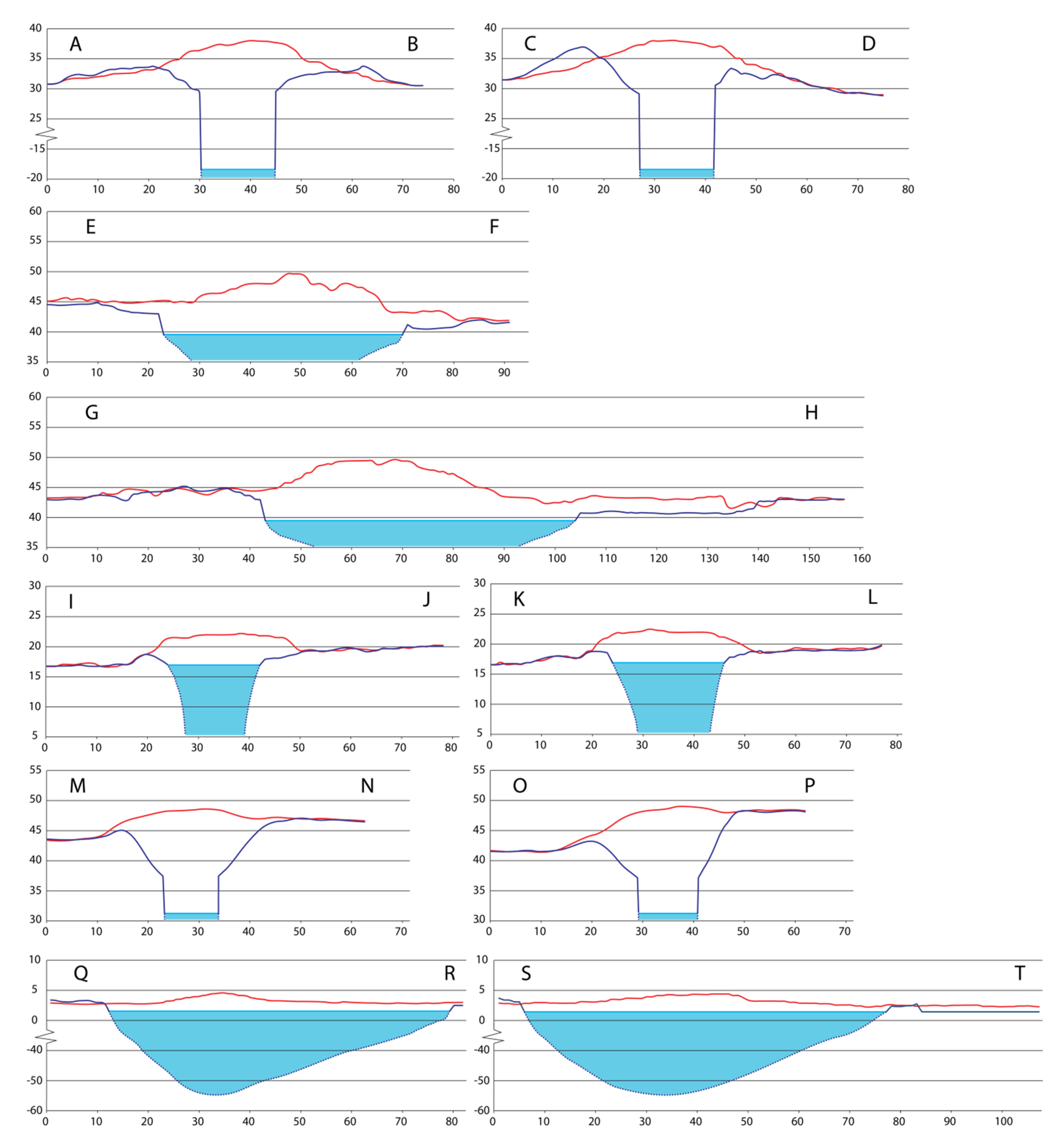
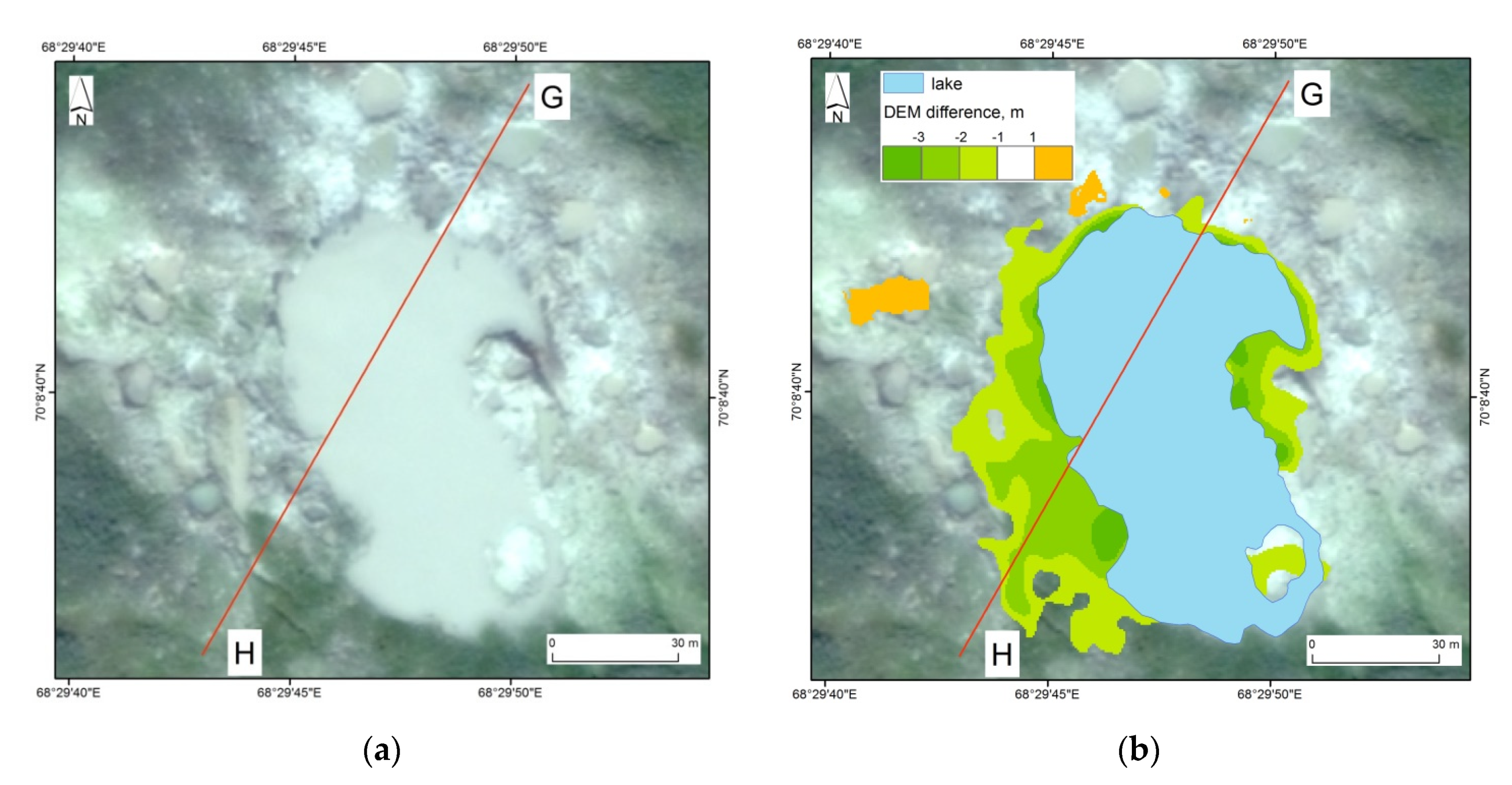
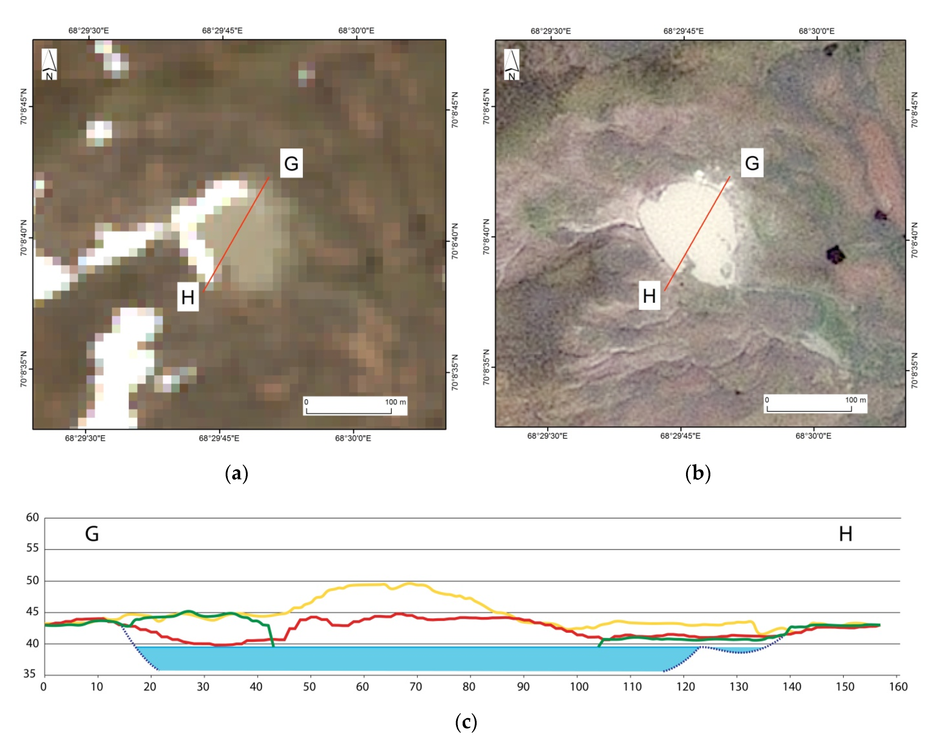
3.2. DSM Interpretation

Field surveys and photographs taken from helicopter prove that GEC-1, GEC-2, and AntGEC have a similar internal structure characterized by a funnel-shaped upper part and a cylindrical lower part [3,4,19,31]. There are no data on the structure of GEC-3 and SeYkhGEC due to the lack of observations, as well as no DSMs covering the timeframe between the formation and inundation of these GECs (GEC-3 was flooded by atmospheric waters and thawing permafrost, and SeYkhGEC was flooded by river waters before first observation was made possible, on 1 July 2017). Diameters across the top edge of the funnel-shaped part of GECs measured at the earliest convenience are presented in Table 3.
Mound-predecessors and the resulting GECs appearance on satellite imagery are presented in Figure 4, as well as the position of transects along which elevation profiles characterizing relief variations are plotted.
Mound-predecessor dimensions were measured using DSMs and elevation profiles derived from DSMs presented in Figure 5. Profile locations are shown in Figure 4. Table 3 presents the morphometric properties of mound-predecessors, their heights ranging between 1.7 and 6 m.
Mounds’ base ranges between 20 to 55 m in diameter. The diameter of SeYkhGEC mound-predecessor was evaluated using the magnitude of the Myudriyakha river channel deformation. In 2016, a year before the GEC appeared, the river channel had formed a meander of about 55 m at a longer axis. Using the ArcticDEM dated 19 April 2016, the difference in heights at the top and foot of mound-predecessor was as high as 1.7 m. Given that snow cover can get thicker downhill at this time of the year, the mound was almost certainly higher than 1.7 m.

3.3. Evaluating Relief Changes—An Estimate of Ejected Material Volume

We have computed the amount of material ejected from GEC-1 and deposited around the perimeter in the form of an accumulative parapet [3]. Our computation relied on the difference between DSMs of 2013 and 2014 (Table 1). The volume of the partially destroyed mound and blocks of frozen deposits thrown out of the GEC are equal to 11,200 m3 while the resulting parapet has a volume of 1940 m3 [3]. The difference between the void volume inside the crater and the volume of the accumulative parapet around the GEC is explained by a significant amount of ice in the ejected frozen blocks that thawed away next summer.
Thus far, GEC-1 remains the only feature promptly surveyed by researchers while still exposed to observation. Among other things, records of key morphometric properties of the resulting GEC were made including its depth. As far as there are no depth data from field surveys on other GECs, we believe it would be incorrect to compute the amount of ejected material and to compare various GECs using this parameter. Depths of resulting GECs cannot be assessed when analyzing stereo pairs of satellite imagery due to the occlusion depending on camera system orientation angles, lighting conditions, and geometry of GECs themselves. We suggest various proxies to estimate the volume of ejected material, such as the volume of the parapet.
Helicopter photographs obtained soon after the formation of GEC-2 clearly show an accumulative parapet in its surroundings together with individual blocks of frozen deposits and ice ejected to the surface [19]. Due to the absence of very-high-resolution stereo pairs showing the parapet at the time of its formation prior to its washing out and inundation of GEC-2, only visual estimates of the parapet volume can be made. Width, average height, and shape of the parapet were measured in field, on photos, and imagery and then approximate volume calculated. Roughly, ejected material was 1/3 to 1/2 less in volume than that for GEC-1.
A comparison of DSMs for the GEC-2 key site before and after the formation of the GEC reveals a zone where the elevation of the surface has decreased (Figure 6). This zone occurs south-west and east of the GEC-2 inner lake. The difference in height between surfaces of different age stands at 2–3 m (GH profile in Figure 5 and Figure 6), which exceeds the relative height accuracy for differences between DSMs (Table 2, last column) to consider this difference as significative. The GEC-2 inner lake measuring 108 × 65 m in size in the photograph dated 21 July 2013, significantly exceeds GEC dimensions of 32 to 35 m in diameter estimated on helicopter photographs from 14 November 2012 [19] and satellite imagery.
There are no field photographs for GEC-3 close to its formation time. DSMs difference confidence level (Table 2) and residual snow accumulations make it impossible to estimate the volume of the accumulative parapet. Yet, we consider that the amount of ejected deposits (excluding melted ice) was less than in the case of GEC-1 and GEC-2. There is no pronounced parapet. Impact landforms do not show up as would have been as a result of the ejection of large frozen blocks.
Lack of information on SeYkhGEC DSM and field data time series does not allow to estimate terrain changes and the amount of ejected material.
Relief changes associated with AntGEC formation were analyzed using DSMs generated earlier [4,5]. Superficial sandy deposits occur widely around AntGEC. It is surrounded by a blanket of ejected sand observed in the field and visible on imagery. No accumulative landforms thicker than 0.9 m were observed. Once thawed, ejected blocks of sand and ice did not leave any clear accumulative forms. Field observation has recorded just blurred spots of sand atop the vegetative cover. For this reason, we were unable to determine the amount of ejected out of this GEC material.
Based on provided data we believe that among all GECs surveyed, GEC-3 and AntGEC had the least amount of material ejected upon their formation.

4. Discussion

4.1. Gas Emission Craters Formation Dates

Landforms under discussion are extremely dynamic. Time span between GEC formation and the closest time of acquisition matters a lot in terms of the crater size, degree of its flooding, and state of the frozen blocks ejected. The fact that this time span differs for various GECs make it complicated to conclude on relations between the parameters of the mound-predecessor and the resulting crater.
The GEC-1 formation timeframe was estimated to be between 9 October and 1 November 2013 (Table 2) based on the analysis of Landsat 8 imagery [16]. Our interpretation of imagery was guided by the following considerations. According to the measurements taken during the field survey on 16 July 2014 [31], as well as interpretation of WorldView-1 images dated 15 June 2014, the rim of GEC-1 was 25–29 m in diameter. As far as this GEC formed in the fall of 2013, since then its rim had retreated from its original size due to the thaw and collapse of its frozen icy walls. Based on a series of multi-temporal images, we suggest that a small (1.5 × 1.5 pixel) dark patch (with low reflectivity) is a GEC that can be interpreted with confidence in images starting 1 November 2013 [3,16]. Simultaneously, a light (high-reflectivity) patch appears on these images. Its spatial position coincides with the accumulative parapet clearly visible on later, very-high-resolution images from the summer of 2014. The expansion of the dark patch until 3 April 2014, can be explained by the fast melting of a thin layer of snow over the accumulative hillocks within the parapet that formed in the fall, 2013. These forms, clearly visible, were the first to expose from the snow.
A publication by Sizov [1] offers another viewpoint concerning GEC-1 formation time using the same Landsat imagery. Sizov concluded that GEC-1 had formed between 21 February and 3 April 2014. Different readings of identical images arise due to small dimensions of the newly formed object relative to image resolution (15 m per pixel). It would be impossible to validate any viewpoint using more detailed imagery as none is found in global operators’ catalogs. Thus, the difference in GEC-1 formation dates remains within the range of 9 October 2013, to 3 April 2014, i.e., the GEC was formed between fall 2013 and spring 2014.
Sizov [1] pointed out that GEC-2 had formed no later than 2 May 2013, by highlighting a depression on a snow-covered Landsat image. Images listed above (Table 2) have enabled to narrow considerably the GEC-2 formation timeframe down to 16 days—between 24 September and 15 October 2012.
The wide GEC-3 formation timeframe between 22 October 2012 and 10 June 2013 (Table 2) is due to a lack of cloud-free images between identified dates with a resolution sufficient for confident interpretation of the newly formed GEC (no more than 15 m per pixel).
There are no discussions concerning AntGEC and SeYkhGEC formation dates in literature, the only source being reports from local citizens pointing particular dates of 27 September 2013, and 28 June 2017, respectively (Table 2).

4.2. Geomorphic and Environmental Patterns Associated with Gas Emission Craters

GECs under study reveal an extremely wide range of geomorphic settings (Table 3). All GECs in the Yamal Peninsula are associated with geodynamic accumulation zones, such as slope foot adjacent to valleys of permanent or temporary streams (GEC-1, GEC-2, GEC-3), or a river channel (SeYkhGEC). Slopes are rather gentle since they are never steeper than 7°. All these areas are low and wet, with increased snow accumulation in winter. In that respect, the only known GEC in the Gydan Peninsula (AntGEC) is different. It is located at the border between a denudation zone and a transit zone downslope, on the edge of a watershed surface. This terrain inflection is sloping at 7–15°, several times steeper than slopes of surfaces where Yamal GECs had formed. AntGEC is the only GEC to form on a well-drained surface with sandy deposits. However, none of the known craters is located in the central part of the watershed surfaces.
Differences noted in the GEC position regarding terrain contradicts the hypothesis proposed in [7,9] stating that the GEC form by exploding of perennial frost mound (known as a bulgunniakh, or pingo, resulting from freezing of a drained lake talik) in a closed system. The existence of such a talik can be assumed under a lake in the area of GEC-1 (even though this GEC is located at the foot of a slope). However, the location of all other GECs (GEC-2, GEC-3, SeYkhGEC, AntGEC) on slopes or in the river channel is not appropriate to the formation of a closed talik that could yield a frost mound upon freezing over.
The height of the mound-predecessors correlates well with the diameter of their base. The exception is the mound-predecessor of SeYkhGEC. Perhaps the overestimated diameter of this mound is since it was determined by ArcticDEM Stripes, based on images dated 19 April 2016, and the foot of the mound was covered with snow.
GECs are actively expanding due to the thaw and collapse of frozen icy walls, and are flooded by water from melted ground ice, snow accumulating inside the craters in winter, and rainfalls. GEC diameters across their rims were determined after different times elapsed after their formation. All the studied GECs have closely matching diameter values within 25–37 m (Table 3). Based on field observations, satellite imagery analysis, and the period between the formation of the GECs and the date the measurements were taken, we believe that all GECs were initially 20–25 m in diameter. It should also be noted that the diameter of the crater is not related to the size of the mound-predecessor. AntGEC had the smallest mound-predecessor with relative height and diameter two to three times less than in other GECs, but the diameter of the resulting crater was the same. Perhaps the similarity of the diameters of the GECs is explained not only by the pressure of gas that led to the formation of the mound-predecessors but also by the mechanical properties of the deformed frozen rocks when bending deformation occurs.
The SeYkhGEC is unique as its mound-predecessor was located immediately next to the Myudriyakha river channel. At SPOT5 images from 2011 and 2012, the river course in the study area is stable and virtually straight with a small indentation on the south-eastern bank (Figure 7). SPOT7 images from 2015 and 2016 showed extensive dynamics of mound growing and river channel bending. After the GEC had formed on 28 June 2017, it was immediately flooded.
Analyzing multi-temporal imagery for SeYkhGEC we suppose that the life cycle of a GEC, including the growth and explosion of its mound-predecessor, can be as short as three–five years (and even shorter for SeYkhGEC; from 2015 to 2017). Similar estimates were made by other researchers who suggested that ground surface deformation started in this area in 2013 with most active motion having occurred between 2015 and 2017 [7]. In comparison, the life cycle of GEC-1 was calculated using dendrochronology at around 65 years [32]. The SeYkhGEC crater appearance supports our conclusion that the extremely warm summer of 2012 was a trigger of several GEC formations. This warming, probably, was insufficient for the blow out of SeYkhGEC mound-predecessor, but only for its growth. Probably, this mound-predecessor experienced “heat-struck” once again during an even warmer summer of 2016, which caused its explosion.
A significant diameter of the Myudriyakha river course expansion observed on a satellite image one month after SeYkhGEC formation can be explained, first, by a considerable force behind material ejection and formation of a huge GEC in the place of a mound-predecessor; and second, by intense destruction of SeYkhGEC walls due to river erosion. Bogoyavlensky et al. [7] mentioned riverbank erosion rates as high as 1.47 m per day immediately after GEC formation.
It should be noted that we disagree with the mechanism of the formation of a mound-predecessor in a river channel proposed in the paper being a frost mound (pingo) [7]. A classical pingo with an ice core is driven by cryostatic or hydraulic pressure. Such conditions do not exist in a river channel where there is a warming effect of water. Talik in the river bottom does not freeze back in winter; thus, cryostatic or hydraulic pressure is not produced. Talik beneath the riverbed would not allow the formation of an ice core through migration or intrusion mechanism. We believe that a positive landform (GEC mound-predecessor) results from surface deformation affected by gas migration and expansion. This process has no relation to classic pingo growth schemes [33,34,35]. Misusing the term “frost mound” (“pingo”) in this case would cause terminology confusion and wrong understanding of the particular origin of the phenomenon under consideration. Better explaining our feature is the term “gas hydrate pingo” used in literature when discussing sea-floor landform-predecessors of pockmarks [36].
The internal structure of GECs was observed in GEC-1, GEC-2, and AntGEC. However, we assume the nature of all GECs to be identical in mechanisms and triggers. Thus, as they were not observed before inundation, SeYkhGEC and GEC-3 most likely had the same structure of cylindrical lower part and funnel-shaped upper part.
The presence of tabular ground ice in GEC walls is a common feature of all GECs. Ice is an important control of GEC formation [17,18,37,38,39]. The release of methane from permafrost (including gas hydrate decomposition) is likely caused by rising air and ground temperature over the past decades. The formation of all GECs was preceded by anomalously warm summers [40,41]. Gas may accumulate in cryopegs below tabular ground ice layers serving as traps [16,42,43]. Irregularities in the tabular ground ice body together with its rough base yield favorable conditions for gas concentration that later causes deformation of ice and overlaying deposits thus forming a mound-predecessor.
We revealed the effect of lowering the surrounding surface only in the vicinity of GEC-2 (Figure 6). A comparison of the DSMs before and after the formation of GEC-2 for this area showed a negative change in height up to 2–3 m (Figure 6b). Part of this area was flooded by lake water. This subsidence of the surface within a radius of 80 m from the crater occurred in the first six months after the formation of GEC-2. During the same half-year, a big lake appeared due to flooding of the crater, with a diameter six–seven times larger than the initial diameter of the crater [20]. Since then, the lake has been increasing in size only due to the thawing and retreat of the steep lake shore in the northern part of the lake [7]. In the southern part of the lake, the shore has not eroded and is represented by a flooded, gently sloping towards the center of the lake surface with grass vegetation emerging through the water (Figure 6a). The position of the shoreline in this part of the lake remained stable as confirmed by comparison of field survey in September 2017 and the 2013 satellite image. Such surface flooding is possible only if a portion of a valley where lake is forming has a reverse sloping of valley profile. We assume that during the explosion of the mound-predecessor in the fall of 2012, gas released and a cavity left in which gas had accumulated beneath the ice layer serving as a trap [17]. Probably, during the explosion, cracks formed in the upper horizons of the frozen deposits, and the blocks settled into the cavity freed from the gas and gas hydrates.

4.3. Applicability of Remote Sensing Data

We conducted raw image processing with DSM extraction. Since various products of satellite images post-processing are in open access, it became necessary to assess the applicability of various types of data to solve our tasks.
DSM relative height accuracy (0.35–1.01 m for GEC-3 and AntGEC, see Table 2) makes up 12–34% for rather low mounds 23 m in height preceding formation of GEC-3 and AntGEC (Table 3). For GEC-1 and GEC-2 mound-predecessors are 4 to 6 m high (Table 3), while the relative height accuracy (0.35–0.45 m) of DSM comprises only 7–10% of their height. Thus, DSMs’ relative height accuracy is crucial for the estimation of lower mounds height, which is rather close to the height accuracy itself.
We also considered the usability of the ArcticDEM covering the Arctic region to identify features linked to GEC formation. ArcticDEM v3.0 with a 2-m spatial resolution is available currently. The comparison between our DSM compiled for GEC-1 (see Table 2) and the ArcticDEM Stripes data, based on the same images, both allowed to identify the mound-predecessor and to determine its morphometric properties (Figure 8). Both products render the mound in a very similar manner with differences only in representing microrelief due to higher spatial resolution of authors’ DSMs. Considering that an example in Figure 8 confirms the local accuracy of mound-predecessor identification, we believe that ArcticDEM Stripes can be used when searching for other mound-predecessors or predicting the occurrence of new GECs.
However, there are limitations concerning the use of this data. These limitations arise due to the automated process used for generating the ArcticDEM without a thorough spatial analysis for possible artifacts on the resulting surfaces. Such artifacts may take place from stereo matching errors in the presence of clouds, cloud shades, and errors associated with waterway surfaces (both open waters and icebound). It is furthermore important to consider the season when stereo pairs for the compilation of ArcticDEM Stripes were obtained as snow cover may camouflage the relief of the initial surface.
For instance, for the GEC-2 site, one may end up with an erroneous conclusion that a new mound had formed in summer 2016 (see Figure 9c, red line) when analyzing multi-temporal data from ArcticDEM Stripes. Remote sensing data (Figure 9) obtained during August 2016 field surveys indicated that there was no mound, while a lake that had formed in the GEC site in 2013 had continued to expand. A Sentinel-2 optical image obtained on the same date as the source images used for ArcticDEM Stripes (16 June 2016) provides a reliable indication of lake water surface with residual signs of snow cover on the western coast (Figure 9a). The lake appears as well on a higher spatial resolution SPOT6 image dated 15 July 2016 (Figure 9b). Thus, the “mound” in ArcticDEM does not match the reality. Though ArcticDEM can generally be used when searching for mound-predecessors, it should be taken into consideration that this DSM in some cases may comprise an artifact most likely caused by errors in the processing of a signal reflected from the water surface.
Multi-temporal ArcticDEM Stripes allows identifying areas with relief changes. If these changes are expressed in the form of appearing or disappearing mounds, then such sites require special attention and thorough analysis. One of the instruments for such an analysis is DSMs compiled from random stereo pairs. They can be used to refine the rate and magnitude of changes in elevation that are fixed in ArcticDEM.
We can state that surface settings, which are confidentially interpreted on satellite imagery, cannot be considered strong attributes characterizing an area of the probable mound and GEC formation. A joint analysis of remote sensing data and the study of the cryolithologic structure infield is required.

5. Conclusions

After the direct observation of gas-emission craters and determining their coordinates, we compiled detailed DSM based on very-high resolution satellite images. We performed a retrospective analysis of changes in the relief, which determined the size and shape of mound-predecessors now ruined by GEC formation. Established are the following similar features of the study objects: (1) all GECs formed in the place of mound-predecessors 2–6 m high and 20–55 m in the base diameter; (2) all mound-predecessors were located on gentle slopes 1 to 15° steep; (3) immediately after formation, GECs were characterized in shape by the lower cylindrical portion and the upper funnel-shaped portion; (4) initial diameter of the upper funnel-shaped portion ranged around 20–25 m; (5) both in the GEC walls and in frozen blocks ejected from the crater, tabular ground ice is observed. Differing features are (1) localization in different elements of relief and a variety of vegetation types; (2) some GECs have accumulative parapet expressed in relief, while others do not; (3) some GECs have impact landforms resulting from huge frozen blocks fallen on the ground surface, while others do not; (4) while GECs 1, 2, and 3 had formed within the clayer deposits, AntGEC and SeYkhGEC appeared within the areas with sandy deposits.
We successfully applied a method of DSM extraction out of random stereo pairs, obtained by different sensing systems as well as from multi-temporal acquisitions. Such random stereo pairs are of high value for retrospective analysis of the study landforms considering a limited number of normal stereo pairs. Using this technique, a series of DSM can be compiled with a frequency exceeding that of ArcticDEM, compiled in an automatic mode based on normal stereo pairs. Relatively small features under study require high-resolution images to compile DSM suitable for obtaining their morphometric parameters with sufficient accuracy.
The rate of mound growth is very high, several years (less than five years for SeYkhGEC mound-predecessor) to several decades (GEC-1 mound-predecessor). That is an additional reason why the high-temporal-resolution DSM time series can help identify the rate of growth and separate the mound-predecessors of GECs from other mounds.
We assume that constantly updated ArcticDEM Stripes’ coverage can be used as a valuable source for automatic detection of both mound-predecessors and gas emission craters because the metric properties of these DSMs are sufficient to indicate changes in the relief, comparable in size with the analyzed objects. Yet, the use of these data has several limitations associated with automatic data processing, which in some cases leads to artifacts. In this regard, mandatory verification of identified objects using optical range images is necessary.
Known gas emission craters are located in a wide range of terrain and environmental conditions—from the drained edge of the terrace, to the foot of the gentle slope, to the bottoms of thermoerosion gullies and river channels. Such variations tentatively indicate a small role of surface conditions including modern relief. Common to the studied gas emission craters is the internal geologic and cryolithologic structure with the presence of tabular ground ice in the crater walls. A combination of tabular ground ice close to the surface with continuous permafrost saturated with methane, and saline deposits below the ice bodies (cryopegs) are altogether a necessary condition for the gas emission craters formation, which is a specific feature of the North of West Siberia only. Probably, for this reason, such GECs are not found elsewhere in permafrost areas ashore.
Thus, a small number of discovered GECs, the importance of geological structure, not quite well detected using remote-sensing, and the little role of environmental settings best indicated by remote-sensing are limitations in the implementation of an algorithm for automatic detection of mounds-predecessors and prediction of new GEC formation.

Author Contributions

Conceptualization, writing—original draft preparation, A.K. (Alexander Kizyakov) and M.L.; methodology, formal analysis, M.Z. and A.S.; investigation, Y.D. and A.K. (Artem Khomutov); project administration, review and editing, D.D., E.C., and Y.S.; funding acquisition, V.P. All authors have read and agreed to the published version of the manuscript.

Funding

Cartographic image analyses and SeYkhGEC data processing as well as APC were funded by the Russian Foundation for Basic Research (RFBR) Project No. 18-05-60221. SPOT5 data for GEC formation timeframe finding were obtained from the shared-use equipment center “Geoportal,” Faculty of Geography, M.V. Lomonosov Moscow State University. GEC-1 satellite imagery were purchased and analyzed as a result of our initiative study supported by the Russian Center for Arctic Development [3]. GEC-2 and GEC-3 satellite imagery were purchased and analyzed under a joint project with energy company Total SA (France) and the Russian Center for Arctic Development. AntGEC data were obtained and processed as a part of the Russian Science Foundation project No.16-17-10203 [4,5]. Terrain dynamics analysis was funded by the Russian Foundation for Basic Research (RFBR) Project No. 18-05-60080. The field data have partially been processed with the support of the “RUDN University programme 5-100”.

Acknowledgments

The authors thank “Russian Center for Arctic Development” for organizing and supporting field work. We thank anonymous reviewers for valuable comments and improvements to the manuscript.

Conflicts of Interest

The authors declare no conflict of interest.

References

  1. Sizov, O.S. Remote sensing data analysis of the consequences of gas releases in the north of Western Siberia. Geomatica 2015, 1, 53–68. [Google Scholar]
  2. Bogoyavlenskiy, V.I.; Sizov, O.S.; Bogoyavlenskiy, I.V.; Nikonov, R.A. Remote identifications of areas of surface gas and gas emissions in the Arctic: Yamal Peninsula. Arct. Ecol. Econ. 2016, 3, 4–15. [Google Scholar]
  3. Kizyakov, A.I.; Sonyushkin, A.V.; Leibman, M.O.; Zimin, M.V.; Khomutov, A.V. Geomorphological conditions of the gas-emission crater and its dynamics in Central Yamal. Earth’s Cryosph. 2015, 19, 13–22. [Google Scholar]
  4. Kizyakov, A.I.; Zimin, M.V.; Sonyushkin, A.V.; Dvornikov, Y.A.; Khomutov, A.V.; Leibman, M.O. Comparison of gas emission crater geomorphodynamics on Yamal and Gydan peninsulas (Russia), based on repeat very-high-resolution stereopairs. Remote Sens. 2017, 9, 1023. [Google Scholar] [CrossRef] [Green Version]
  5. Kizyakov, A.I.; Sonyushkin, A.V.; Khomutov, A.V.; Dvornikov, Y.A.; Leibman, M.O. Assessment of the relief-forming effect of the Antipayuta gas emission crater formation using satellite stereo pairs. Curr. Probl. Remote Sens. Earth Space 2017, 14, 67–75. [Google Scholar] [CrossRef]
  6. Bogoyavlenskiy, V.I.; Bogoyavlenskiy, I.V.; Nikonov, R.A. Results of aerial, space and field investigations of large gas blowouts near Bovanenkovo field on Yamal peninsula. Arct. Ecol. Econ. 2017, 3, 4–17. [Google Scholar] [CrossRef]
  7. Bogoyavlensky, V.I.; Sizov, O.S.; Bogoyavlensky, I.V.; Nikonov, R.A.; Kargina, T.N. Earth degassing in the arctic: Comprehensive studies of the distribution of frost mounds and thermokarst lakes with gas blowout craters on the Yamal Peninsula. Arct. Ecol. Econ. 2019, 4, 52–68. [Google Scholar] [CrossRef] [Green Version]
  8. Khilimonyuk, V.Z.; Ospennikov, E.N.; Buldovicz, S.N.; Gunar, A.Y.; Gorshkov, E.I. Geocryological conditions of Yamal crater location. In Proceedings of the 5th Russian Conference on Geocryologists, Lomonosov Moscow State University, Moscow, Russia, 14–17 June 2016; pp. 245–255. (In Russian). [Google Scholar]
  9. Buldovicz, S.N.; Khilimonyuk, V.Z.; Bychkov, A.Y.; Ospennikov, E.N.; Vorobyev, S.A.; Gunar, A.Y.; Gorshkov, E.I.; Chuvilin, E.M.; Cherbunina, M.Y.; Kotov, P.I.; et al. Cryovolcanism on the Earth: Origin of a Spectacular Crater in the Yamal Peninsula (Russia). Sci. Rep. 2018, 8, 13534. [Google Scholar] [CrossRef]
  10. ArcticDEM Data. Available online: https://www.pgc.umn.edu/data/arcticdem/ (accessed on 17 February 2020).
  11. Bogoyavlenskiy, V.I.; Bogoyavlenskiy, I.V.; Nikonov, R.A.; Sizov, O.S. Technologies for remote detection and monitoring of the Earth degassing in the Arctic: Yamal Peninsula, Neito Lake. Arct. Ecol. Econ. 2018, 30, 83–93. [Google Scholar] [CrossRef]
  12. Dubikov, G.I. Composition and Cryogenic Structure of the Western Siberia Permafrost, 2nd ed.; GEOS: Moscow, Russia, 2002. [Google Scholar]
  13. Yakushev, V.S. Natural Gas and Gas Hydrates in Cryolithozone; VNIIGAZ: Moscow, Russia, 2009. [Google Scholar]
  14. Vasiliev, A.A.; Streletskaya, I.D.; Melnikov, V.P.; Oblogov, G.E. Methane in ground ice and frozen quaternary deposits of Western Yamal. Dokl. Earth Sci. 2015, 465, 1289–1292. [Google Scholar] [CrossRef]
  15. Kraev, G.N.; Schulze, E.D.; Yurova, A.; Kholodov, A.; Chuvilin, E.M.; Rivkina, E.M. Cryogenic displacement and accumulation of biogenic methane in frozen soils. Atmosphere 2017, 6, 105. [Google Scholar] [CrossRef] [Green Version]
  16. Leibman, M.O.; Kizyakov, A.I.; Plekhanov, A.V.; Streletskaya, I.D. New permafrost feature—Deep crater in Central Yamal (West Siberia, Russia) as a response to local climate fluctuations. Geogr. Environ. Sustain. 2014, 7, 68–79. [Google Scholar] [CrossRef]
  17. Streletskaya, I.D.; Leibman, M.O.; Kizyakov, A.I.; Oblogov, G.E.; Vasiliev, A.A.; Khomutov, A.V.; Dvornikov, Y.A. Ground ice and its role in the formation of gas-emission crater in the Yamal peninsula. Mosc. Univ. Bull. Ser. 5geogr. 2017, 2, 91–99. [Google Scholar]
  18. Leibman, M.O.; Kizyakov, A.I.; Streletskaya, I.D. Yamal crater—A new natural and permafrost phenomenon. In Proceedings of the XXI International conference on Marine Geology: Geology of seas and oceans, Moscow, Russia, 16–20 November 2015; IO RAS: Moscow, Russia, 2015; pp. 273–277. [Google Scholar]
  19. Leibman, M.O.; Dvornikov, Y.A.; Khomutov, A.V.; Babkin, E.M.; Babkina, E.A.; Vanshtein, B.G.; Kizyakov, A.I.; Oblogov, G.E.; Semenov, P.B.; Streletskaya, I.D. Hydro-chemical features of water in lakes and gas-emission craters embedded in the marine deposits of West-Siberian North. In Proceedings of the XXII International Conference on Marine Geology: Geology of Seas and Oceans, Moscow, Russia, 20–24 November 2017; Lisitsyn, A.P., Politova, N.V., Shevchenko, V.P., Eds.; IO RAS: Moscow, Russia, 2017; pp. 117–120. [Google Scholar]
  20. Kizyakov, A.I.; Khomutov, A.V.; Zimin, M.V.; Khairullin, R.R.; Babkina, E.A.; Dvornikov, Y.A.; Leibman, M.O. Microrelief associated with gas emission craters: Remote-sensing and field-based study. Remote Sens. 2018, 10, 677. [Google Scholar] [CrossRef] [Green Version]
  21. Porter, C.; Morin, P.; Howat, I.; Noh, M.-J.; Bates, B.; Peterman, K.; Keesey, S.; Schlenk, M.; Gardiner, J.; Tomko, K.; et al. ArcticDEM. Available online: https://dataverse.harvard.edu/dataset.xhtml?persistentId=doi:10.7910/DVN/OHHUKH (accessed on 2 November 2019).
  22. Zimin, M.V.; Sonyushkin, A.V. Automated System for VHR Satellite imagery processing. L. Manag. Cadastrel. Monit. 2014, 1, 38–43. [Google Scholar]
  23. Sonyushkin, A.V. Comparison of DSM creation methods from high spatial resolution stereopairs. Izv. Vuzov. Geod. Aerophotosurveying 2015, 1, 43–52. [Google Scholar]
  24. Hirshmuller, H. Accurate and efficient stereo processing by semi-global matching and mutual information. In Proceedings of the IEEE Conference on Computer Vision and Pattern Recognition (CVPR), San-Diego, CA, USA, 20–26 June 2005; pp. 807–814. [Google Scholar]
  25. Hirshmuller, H. Stereo processing by semi-global matching and mutual information. IEEE Trans. Pattern Anal. Mach. Intell. 2008, 2, 328–341. [Google Scholar] [CrossRef]
  26. Hirshmuller, H.; Buder, M.; Ernst, I. Memory efficient semi-global matching. In Proceedings of the XXII Congress of the International Society for Photogrammetry and Remote Sensing, Melbourne, Australia, 25 August–1 September 2012; pp. 371–376. [Google Scholar]
  27. Sonyushkin, A.V. Improving the Technology for Orthophoto Creating from High-Resolution Space Images. Ph.D. Thesis, Moscow State University of Geodesy and Cartography (MIIGAiK), Moscow, Russia, 2015. [Google Scholar]
  28. Burrough, P.A.; McDonell, R.A. Principles of Geographical Information Systems; Oxford University Press: New York, NY, USA, 1998. [Google Scholar]
  29. Bochkarev, V.S.; Braduchan, Y.V.; Voronin, A.S.; Generalov, P.P.; Kovrigina, E.K.; Kulakhmetov, N.K.; Mitusheva, V.S.; Stavitsky, B.P.; Faybusovich, Y.E.; Shemraeva, S.V. State Geological Map of the Russian Federation. Scale 1:1,000,000 (New Series). Sheet R-43-(45)—Gydan-Dudinka. Explanatory Note; VSEGEI: St. Petersburg, Russia, 2000; 187p. (In Russian) [Google Scholar]
  30. Vasilchuk, Y.K.; Trofimov, V.T.; Badu, Y.B. East-Yamal region. In Geocryology of USSR. Western Siberia; Ershov, E.D., Ed.; Nedra: Moscow, Russia, 1989; pp. 172–180. [Google Scholar]
  31. Leibman, M.O.; Plekhanov, A.V. The Yamal gas emission crater: Results of preliminary survey. KholodOK 2014, 2, 9–15. [Google Scholar]
  32. Arefyev, S.P.; Khomutov, A.V.; Ermokhina, K.A.; Leibman, M.O. Dendrochronologic reconstruction of gas-inflated mound formation at the Yamal crater location. Earth’s Cryosph. 2017, 5, 89–100. [Google Scholar] [CrossRef]
  33. Van Everdingen, R. Multi-Language Glossary of Permafrost and Related Ground-Ice Terms, 2nd ed.; National Snow and Ice Data Center: Boulder, CO, USA, 2005. [Google Scholar]
  34. French, H. The Periglacial Environment, 4th ed.; Hoboken, N.J., Ed.; Wiley-Blackwell: Oxford, UK, 2017; ISBN 9781119132790. [Google Scholar]
  35. Romanovsky, V.E.; Isaksen, K.; Drozdov, D.S.; Anisimov, O.; Instanes, A.; Leibman, M.O.; McGuire, A.D.; Shiklomanov, N.; Smith, S.; Walker, D. Changing permafrost and its impacts. In Snow, Water, Ice and Permafrost in the Arctic (SWIPA); Arctic Monitoring and Assessment Programme (AMAP): Oslo, Norway, 2017; pp. 65–102. [Google Scholar]
  36. Serié, C.; Huuse, M.; Schødt, N.H. Gas hydrate pingoes: Deep seafloor evidence of focused fluid flow on continental margins. Geology 2012, 3, 207–210. [Google Scholar] [CrossRef]
  37. Leibman, M.; Dvornikov, Y.; Khomutov, A.; Kizyakov, A.; Vanshtein, B. Main results of 4-year gas-emission crater study. In Proceedings of the 5 th European Conference On Permafrost—Book of Abstracts, Chamonix, France, 23 June–1 July 2018; Deline, P., Bodin, X., Ravanel, L., Eds.; Laboratoire EDYTEM, CNRS, Université Savoie Mont-Blanc: Le Bourget, France; pp. 293–294. [Google Scholar]
  38. Leibman, M.O.; Dvornikov, Y.A.; Kizyakov, A.I.; Khairullin, R.R.; Khomutov, A.V. Principles and cartographic modeling of the danger associated with of gas emission craters occurrence on the Yamal Peninsula. In Proceedings of the XXIII International conference on Marine Geology: Geology of seas and oceans, Moscow, Russia, 18–22 November 2019; IO RAS: Moscow, Russia, 2019; pp. 263–267. [Google Scholar]
  39. Leibman, M.O.; Kizyakov, A.I.; Dvornikov, Y.A.; Khairullin, R.R.; Khomutov, A.V.; Babkina, E.A.; Streletskaya, I.D. Gas-emission craters puzzle—4 years of investigations. In Proceedings of the Solving the puzzles from Cryosphere: Program, Abstracts, Pushchino, Russia, 15–18 April 2019; pp. 27–28. [Google Scholar]
  40. Khomutov, A.V.; Leibman, M.O.; Gubarkov, A.A.; Dvornikov, Y.A.; Mullanurov, D.R.; Babkin, E.M.; Babkina, E.A. Monitoring of permafrost zone: New data from Cenyral Yamal and arrangement of observation on Gydan. Nauchniy Vestn. Yamalo-Nenetskogo Avton. Okruga 2016, 4, 17–19. [Google Scholar]
  41. Babkina, E.A.; Leibman, M.O.; Dvornikov, Y.A.; Fakashchuk, N.Y.; Khairullin, R.R.; Khomutov, A.V. Activation of cryogenic processes in central Yamal as a result of regional and local change in climate and thermal state of permafrost. Russ. Meteorol. Hydrol. 2019, 44, 283–290. [Google Scholar] [CrossRef]
  42. Leibman, M.O.; Kizyakov, A.I. A new natural phenomenon in permafrost. Priroda 2016, 2, 15–24. [Google Scholar]
  43. Dvornikov, Y.A.; Leibman, M.O.; Khomutov, A.V.; Kizyakov, A.I.; Semenov, P.B.; Bussmann, I.; Babkin, E.M.; Heim, B.; Portnov, A.; Babkina, E.A.; et al. Gas-emission craters of the Yamal and Gydan peninsulas: A proposed mechanism for lake genesis and development of permafrost landscapes. Permafr. Periglac. Process. 2019, 146–162. [Google Scholar] [CrossRef] [Green Version]
Figure 1. Gas emission craters location map.
Remotesensing 12 02182 g001
Figure 2. Differences in the geomorphic setting of gas emission craters identified through DSM analysis. Key site DSM fragments: (a) GEC-1, (b) GEC-2, (c) GEC-3, (d) AntGEC. Red circles indicate GEC location.
Remotesensing 12 02182 g002
Figure 3. SeYkhGEC location on ArcticDEM fragment (red circle). The river pattern was digitized using the SPOT7 image dated 27 July 2017.
Remotesensing 12 02182 g003
Figure 4. Satellite images before (left frame) and after (right frame) gas emission craters formation. GEC-1: (a) WorldView-1 image dated 09 June 2013 (pan) (mound in the center); (b) WorldView-1 image dated 15 June 2014 (pan) (crater with parapet in the center). GEC-2: (c) WorldView-2 image dated 11 September 2011 (synthesis of Red+Green+Blue) (mound in the center); (d) WorldView-2 image dated 21 July 2013 (synthesis of Red+Green+Blue) (inner lake in the center). GEC-3: (e) WorldView-1 image dated 09 June 2011 (pan) (mound in the center); (f) WorldView-2 image dated 10 June 2013 (synthesis of Red+Green+Blue) (inner lake in the center). AntGEC: (g) WorldView-2 image dated 21 August 2013 (pan) (mound in the center); (h) WorldView-1 image dated 11 October 2014 (pan) (crater in the center). SeYkhGEC: (i) SPOT7 image dated 19 July 2016 (synthesis of NIR+Red+Green) (mound in the center); (j) SPOT7 image dated 27 July 2017 (synthesis of NIR+Red+Green) (riverbed expansion in the center). Red lines indicate a position and letter designation of elevation profiles shown in Figure 5.
Remotesensing 12 02182 g004aRemotesensing 12 02182 g004b
Figure 5. Elevation profiles across mound-predecessors and gas emission craters. Profile locations are shown in Figure 4. Profiles were plotted across GEC-1 (AB, CD), GEC-2 (EF, GH), GEC-3 (IJ, KL), and AntGEC (MN, OP) using the created DSMs, listed in Table 1. Profiles across SeYkhGEC (QR, ST) were plotted using 2-m spatial resolution ArcticDEM Stripes created based on images dated 19 April 2016 and 27 June 2017. The red line reflects the morphology of mound-predecessors, and the cyan line shows the morphology of GEC on dates closest to GEC formation as shown in Table 1. The light-blue shaded area presents a lake formed inside the GEC. Lake depth is obtained in the field. SeYkhGEC in the riverbed of the Myudriyakha river is shown to exceed 50 m in depth according to [7].
Remotesensing 12 02182 g005
Figure 6. The difference between DSMs obtained “before” (2010–2011) and “after” (2013) GEC-2 formation): (a) WorldView-2 image dated 21 July 2013; (b) A fragment of DSM difference. Differences in elevation predominantly occur in a well-defined area, located southwest of the lake. See the GH profile in Figure 5.
Remotesensing 12 02182 g006
Figure 7. Changes in the morphology of the Myudriyakha river channel associated with the mound-predecessor growth and formation of SeYkhGEC. The upper row shows fragments of SPOT5 satellite imagery (5 m GSD, pan) while the middle and lower rows show imagery from SPOT7 (1.5 m GSD, synthesis of NIR+Red+Green).
Remotesensing 12 02182 g007
Figure 8. A comparison of elevation profiles plotted using the author’s DSM for GEC-1 (1), with ArcticDEM (2). Both lines are not smoothened. Figure 2a shows the spatial position of the profile AB across the GEC-1 mound-predecessor.
Remotesensing 12 02182 g008
Figure 9. Validating the reliability of a “mound” observed in the GEC-2 location using ArcticDEM Stripe of 2016: (a) Surface conditions on 16 June 2016, based on Sentinel-2 image; (b) Surface conditions on 15 July 2016, based on SPOT6 image; (c) Elevation profiles: the red line is the surface plotted using ArcticDEM Stripe extracted from a 16 June 2016 imagery; the yellow line is the mound-predecessor surface “before” GEC formation extracted from multi-temporal stereo pair of 2010–2011 (Table 1); the green line is the surface “after” GEC formation on 21 July 2013 (Table 1); water surface boundaries are shown as of SPOT6 image dated 15 July 2016.
Remotesensing 12 02182 g009
Table 1. Gas emission craters formation timeframe.
Time FrameDateSensorPan Ground Sample Distance (GSD), m
GEC-1 (Yamal Peninsula)
before09 October 2013Landsat 815
after01 November 2013Landsat 815
GEC-2 (Yamal Peninsula)
before24 September 2012SPOT55.5
after15 October 2012SPOT55.3
GEC-3 (Yamal Peninsula)
before22 October 2012SPOT52.5
after10 June 2013WorldView-20.5
SeYkhGEC GEC (Yamal Peninsula)
formed on 28 June 2017 defined by observation
AntGEC (Gydan Peninsula)
formed on 27 September 2013 defined by observation
Table 2. Satellite imagery used for digital surface model (DSM) extraction.
SensorDateMean Scan Azimuth AngleMean Scan Elevation AngleOrbit Height (H), kmPan Ground Sample Distance (GSD), mEstimated Relative Height Accuracy of the DSMs, mDSMs Difference Confidence Level, m
GEC-1 (Yamal Peninsula)
WorldView-19 June 2013307.964.94400.5800.450.57
WorldView-19 June 2013196.867.44400.563
WorldView-115 June 2014184.166.54400.5400.35
WorldView-115 June 201437.464.04400.579
GEC-2 (Yamal Peninsula)
GeoEye-130 July 201050.372.07700.4500.390.52
WorldView-211 September 2011258.971.17700.506
WorldView-221 July 2013230.362.87700.5510.35
WorldView-221 July 20132.968.97700.514
GEC-3 (Yamal Peninsula)
WorldView-105 June 201160.872.64400.5401.011.07
WorldView-109 June 2011114.984.64400.509
WorldView-210 June 2013357.958.97700.5780.36
WorldView-210 June 2013253.661.87700.557
AntGEC (Gydan Peninsula)
WorldView-221 August 201327.577.07700.480.350.65
WorldView-221 August 2013205.860.07700.55
WorldView-111 October 2014335.964.84400.580.55
WorldView-111 October 2014258.163.64400.62
Table 3. Comparison of geomorphic and environmental characteristics of studied landforms.
CharacteristicsGEC-1GEC-2GEC-3SeYkhGECAntGEC
Before GEC Formation
Mound height, m5–64–631.72
Mound diameter, m45–4840–5536–465520
Mound interpretation on imagesSemi-spheric structure. Represented by a high-center polygon that rises above the surrounding polygonal surface
Local relief featuresThe gentle slope foot of a hill next to the drained lake depressionThe upper portion of the erosion- thermokarst valleySlope foot, close to the poorly expressed river floodplainPoint barThe edge of the terrace bending into the slope of the thermoerosion hollow
Slope angle1–7°1–3°3–7°1–3°7–15°
After GEC Formation
Dates of GEC formationFall 2013Fall 2012Fall 2012–spring 2013Summer 2017Fall 2013
GEC edge diameter, m25–2932–3535–3776–88 125–28
GECs’ inner structureThe lower cylindrical portion and the upper funnel-shaped portionNo dataThe lower cylindrical portion and the upper funnel-shaped portion
Tabular ground iceExposed in GEC wallsSeen on photographs of ejected materialNo dataSeen on photographs of ejected materialExposed in GEC walls
1 River course expansion diameter.

