TROPOMI NO₂ Tropospheric Column Data: Regridding to 1 km Grid-Resolution and Assessment of their Consistency with In Situ Surface Observations

Abstract

This work presents a regridding procedure applied to the nitrogen dioxide (NO₂) tropospheric column data, derived from the Copernicus Sentinel 5 Precursor Tropospheric Monitoring Instrument (S5P/TROPOMI). The regridding has been performed to provide a better comparison with punctual surface observations. It will be demonstrated that TROPOMI NO₂ tropospheric column data show improved consistency with in situ surface measurements once the satellite retrievals are scaled to 1 km spatial sampling. A geostatistical technique, i.e., the ordinary kriging, has been applied to improve the spatial distribution of Level 2 TROPOMI NO₂ data, which is originally sparse and uneven because of gaps introduced by clouds, to a final spatial, regular, sampling of 1 km × 1 km. The analysis has been performed for two study areas, one in the North and the other in the South of Italy, and for May 2018-April 2020, which also covers the period January 2020-April 2020 of COVID-19 diffusion over the Po Valley. The higher spatial sampling NO₂ dataset indicated as Level 3 data, allowed us to explore spatial and seasonal data variability, obtaining better information on NO₂ sources. In this respect, it will be shown that NO₂ concentrations in March 2020 have likely decreased as a consequence of the lockdown because of COVID-19, although the far warmest winter season ever recorded over Europe in 2020 has favored a general NO₂ decrease in comparison to the 2019 winter. Moreover, the comparison between NO₂ concentrations related to weekdays and weekend days allowed us to show the strong correlation of NO₂ emissions with traffic and industrial activities. To assess the quality and capability of TROPOMI NO₂ observations, we have studied their relationship and correlation with in situ NO₂ concentrations measured at air quality monitoring stations. We have found that the correlation increases when we pass from Level 2 to Level 3 data, showing the importance of regridding the satellite data. In particular, correlation coefficients of Level 3 data, which range between 0.50–0.90 have been found with higher correlation applying to urban, polluted locations and/or cities.

1. Introduction

Nitrogen dioxide (NO₂) and nitrogen oxide (NO), together indicated as nitrogen oxides (NOx = NO + NO₂), are significant trace gases in the Earth’s atmosphere. They are emitted in the atmosphere because of natural (lightning, fires, soil microbial processes) and anthropogenic (traffic, biomass and fuel combustion) processes and/or activities. In the presence of sunlight, NO is converted into NO₂ through a photochemical process involving ozone (O₃) on a time scale of minutes. For this reason, NO₂ can be considered as a robust measure for concentrations of NOx [1]. NO₂ is a trace gas present in both the troposphere and stratosphere. The tropospheric NO₂ is a pollutant, which can severely affect air quality; hence, human health [2]. The gas has a strong reactivity, especially in the presence of OH, and contributes to the formation of tropospheric ozone and aerosol [3,4,5].

In the stratosphere, NO₂ is mainly produced from the oxidation of nitrous oxide (N₂O). The stratospheric NO₂ enters important catalytic reactions, which can destroy the ozone layer [6] but can also suppress ozone depletion by converting hydrogen compounds into unreactive reservoir species such as nitric acid (HNO₃), that constitutes one of the significant aerosol sources. Tropospheric NO₂ is mainly present in polluted regions, where it can account for 50%–90% of the total column amount [7].

Moreover, we know (e.g., [8,9,10,11,12,13,14,15,16]) that the daily evolution of the Planetary Boundary Layer (PBL) height can affect the vertical mixing ration profile of NO₂ and its diurnal cycle. The PBL height can at most reach an altitude of 1–3 km (e.g., [11,12]); usually, it rapidly increases in the morning because of sunlight and tends to stay at or below ≈1000 m at night. Above the PBL, NO₂ concentrations approach zero (e.g., [11]). Apart from short-time scale events such as tropospheric lightning and aviation traffic, the main sources of NO₂ are at or near the ground. As a result of the evolving PBL and the intense photochemical activity of nitrogen dioxide, its concentration near the surface tends to decrease in sunlight.

For this reason, satellite observations need to discriminate between tropospheric and stratospheric nitrogen dioxide to get a better insight into detecting pollution in the lower atmosphere. In this respect, satellite observations are usually performed in the UV–VIS spectral regions to exploit the absorption mode remote sensing, which has weighting functions, which do not drop to zero at the surface. Examples of instrument sensing the near-surface in absorption mode include the Global Ozone Monitoring Experiment (GOME), onboard the European Remote Sensing 2 (ERS-2) satellite [17,18], the Scanning imaging Absorption Spectrometer for Atmosphere Chemistry (SCIAMACHY), aboard the Envisat satellite, launched in 2002 [19]. Today, tropospheric NO₂ is monitored from space with a series of instruments, such as the Ozone Monitoring Instrument or OMI, launched aboard the Earth Observing System (EOS)—Aura in 2004 [20], the GOME-2 instruments onboard EUMETSAT’s Meteorological Operational Satellites (MetOp) A, B and C launched in 2006, 2012 and 2018, respectively [21] and the TROPOMI instrument, in orbit aboard the Sentinel 5 Precursor in 2017 [22].

As regards the NO₂ data obtained by the predecessors of TROPOMI, such as the OMI instrument, various downscaling techniques have been introduced to improve their spatial resolution. In [23], for example, a downscaling technique applied to OMI NO₂ vertical column density (VCD) data has been developed, using regional air quality model information and also applying averaging kernel (AK) information to adjust the vertical structure. Results have shown best agreement with ground-based observations when downscaling and AK are applied to OMI NO₂, with a correlation coefficient of R $=0.89$. In [24] an approach to improve the spatial resolution of OMI NO₂ data, by applying local scaling factors from a global three-dimensional model, has been presented. Validation results show that the correlation between OMI-derived surface NO₂ and the ground-based measurements, above all in polluted areas, is significant ($R^2\cong 0.86$). Moreover, there are several works based on regression techniques. For example, in [25] a land-use regression technique to OMI NO₂ data has been applied. In particular, in situ concentration measurements and information about surrounding land-uses to estimate concentrations for non-measurement locations were used. In [26] a land-use regression technique was also used for estimating within-urban variability in air pollution at a spatial resolution of 100 m. In [27] the spatial resolution of OMI NO₂ was improved through the combined use of a geostatistical technique, the universal kriging, and a land-use regression technique. Other studies, instead, exploit the information relating to the air mass factor, a value needed to convert the slant column measurement into a vertical column amount, to obtain a high resolution of NO₂ data. Between these, in [28] a high spatial resolution model simulation was used, constrained by in situ aircraft observations, to calculate tropospheric air mass factors and to better estimate tropospheric NO₂ data. All the above studies demonstrated that downscaled NO₂ data better capture the spatial variability compared to the original datasets.

In this work, a regridding technique has been, instead, applied to the newly available Sentinel-5P/TROPOMI NO₂ tropospheric column data. In particular, month averaged NO₂ data have been re-gridded from the TROPOMI spatial resolution (7 km × 3.5 km at the sub-satellite point) to the finer resolution of 1 km × 1 km, obtaining Level 3 data, to possibly improve their accuracy and capture the spatial variability to an even more appreciable spatial sampling. The chosen regridding technique is the ordinary kriging, a geostatistical technique that respect to other approaches, provide several advantages, such as the capability to provide both data estimations and associated errors and of giving satisfactory results also in the presence of few input data. Moreover, the main advantage of the kriging with respect to other deterministic techniques lies in the fact that not only information from geometric distribution of the known points is used, but also the knowledge of the spatial structure of the correlation between observations. The results allowed us to analyze the monthly variability of NO₂ concentration concerning two study areas, one in the North and the other in the South of Italy, and also to highlight different levels of NO₂ comparing weekdays and weekend days, and, finally, COVID-19 (Corona Virus Disease 2019) to non-COVID-19 times.

In addition, the correlation between satellite-based NO₂ data and in situ NO₂ concentrations measured by different air quality monitoring stations have also been analyzed. Recent work has already dealt with this issue finding a significant correlation ($R^2=0.68$) between Level 2 TROPOMI NO₂ products and ground-based observations and a weekend NO₂ level smaller than those observed during weekdays by about 30% in Helsinki [29]. OMI NO₂ observations have also been used to examine the NO₂ weekly load over urban cities [30,31].

Both TROPOMI NO₂ Level 2 and Level 3 data have been correlated against ground-based observations. In particular, ten air quality monitoring stations were considered for the area in the North of Italy, while thirty-seven air quality monitoring stations for the area in the South of Italy.

The paper is organized as follows: Section 2 provides a description of the data used for the implementation and the validation of the regridding procedure; it also describes the applied methodology, focusing on the construction of the empirical semi-variogram. Section 3 shows the results obtained from the application of the regridding method to Level 2 TROPOMI NO₂ data and their validation. In Section 4 we further discuss our results and methodology, and finally, conclusions are drawn in Section 5.

2. Materials and Methods

2.1. TROPOMI NO₂ Observations

TROPOMI is a single payload on board of the Copernicus S5P, one of the European Sentinel satellites dedicated to the monitoring of atmospheric composition, launched on the 13 October 2017. S5P is a near-polar sun-synchronous orbit satellite flying at an altitude of 817 km with an overpass time at ascending node of 13:30 and a repeat cycle of 17 days. TROPOMI operates in a push-broom configuration with a wide swath of about 2600 km, along-track of 7 km, which became 5.6 km from 6 August 2019, and a daily global coverage [32]. The instrument is a four spectrometers system that measures in the ultraviolet (UV), UV–visible (UV–VIS), near-infrared (NIR) and shortwave infrared (SWIR) spectral bands. From these spectral bands, several important air quality and climate-related atmospheric constituents can be retrieved, including NO₂. In particular, the NO₂ columns retrieval algorithm developed by the Royal Netherlands Meteorological Institute (KNMI) exploits the UV–VIS TROPOMI measurements in the 405–465 nm wavelength range [33]. The TROPOMI NO₂ processing system is based on the DOMINO, an algorithm previously used for the OMI instrument [1,34,35]. The retrieval of the total NO₂ slant column density from the Level-1b radiance and irradiance spectra measured by TROPOMI is based on a Differential Optical Absorption Spectroscopy (DOAS) method [36]. The NO₂ slant column density is separated into a stratospheric and a tropospheric part based on information coming from a data assimilation system based on the TM5-MP chemical transport model. Tropospheric and stratospheric slant column densities are converted into vertical column densities by applying an appropriate air-mass factor (AMF) based on a look-up table of altitude-dependent AMFs and information on the vertical distribution of NO₂ from the TM5-MP chemistry transport model at a resolution of 1 × 1 degree and a time step of 30 min [37]. The altitude-dependent AMF depends on the satellite geometry, terrain height, cloud fraction and height and surface albedo.

In this work, the reprocessed Level 2 NO₂ tropospheric column data for the period May 2018–April 2020 have been used. The reprocessed version is the latest version of data that ensures uniformity of the data processing [1,38]. Two other versions of data are also available: the near-real-time stream, available within 3 h after data acquisition, and the offline stream, available within a few days after acquisition. A useful variable contained in NO₂ products, the quality assurance value ($qa\_value$), a continuous variable ranging from 0 to 1, was also taken into consideration. In particular, a $qa\_value$ greater than 0.75, recommended removing cloud scenes covered by snow/ice, errors and problematic retrievals, was used as a pixel filter.

The two target areas are shown in Figure 1 and Figure 2. The first area is the Po Valley, located in the North of Italy (Figure 1, yellow box), bounded in longitude between 7° E and 13° E and in latitude between 44° N and 46° N. The second region is located in the South of Italy (Figure 2, yellow box), bounded in longitude between 13° E and 19° E and in latitude between 39° N and 42° N.

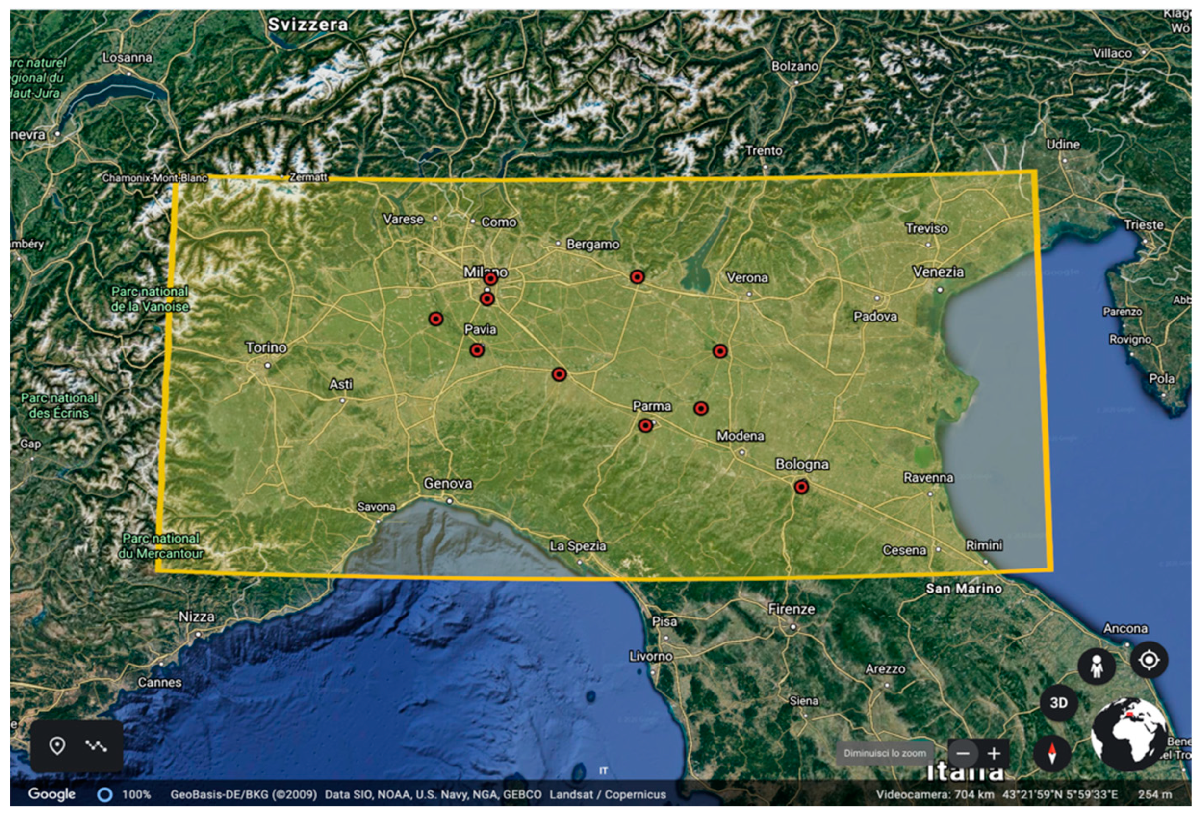
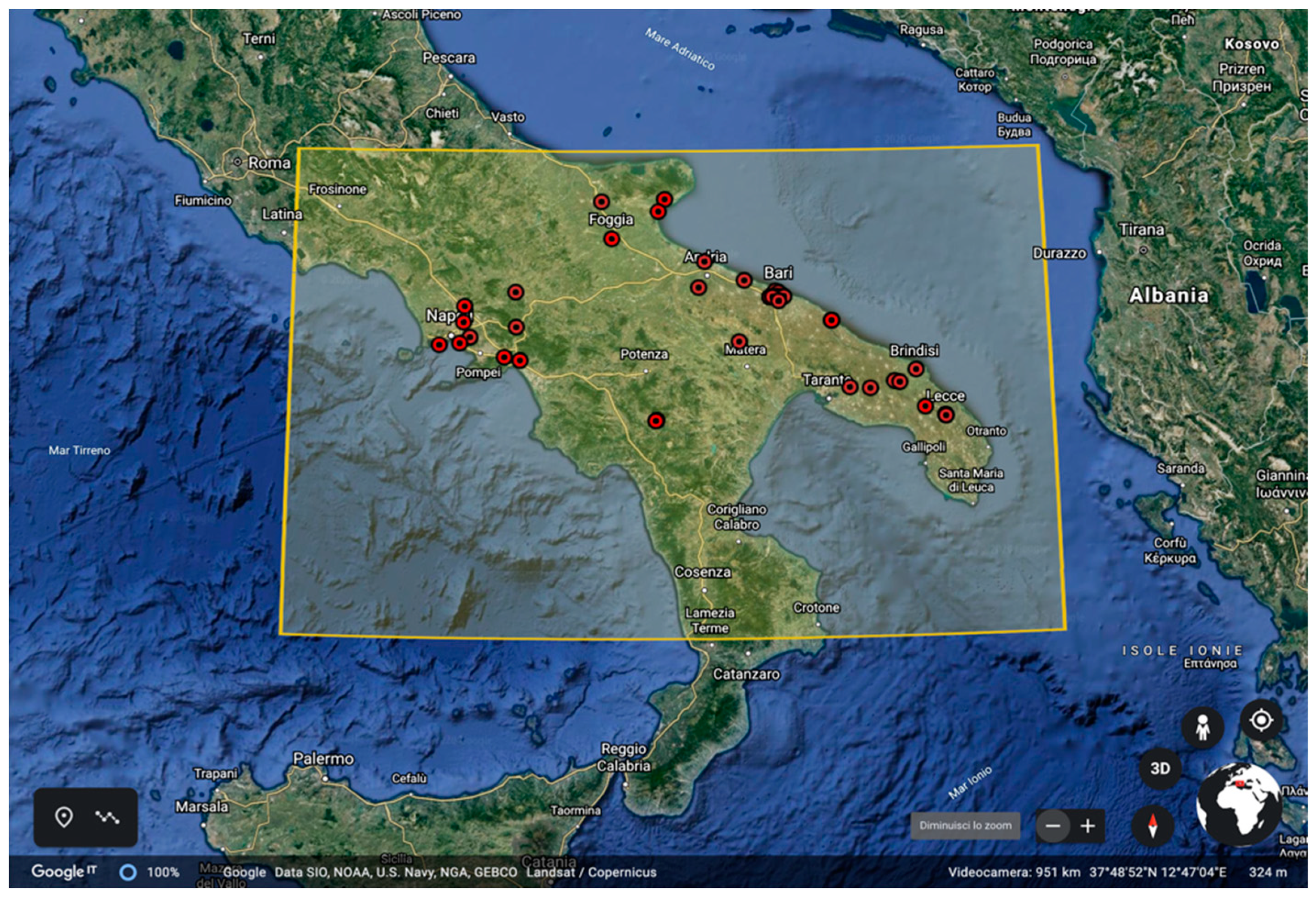
2.2. Ground-Based Observations

For inter-comparison and validation, both Level 2 and Level 3 NO₂ TROPOMI data are compared vs. NO₂ observations obtained by air quality monitoring stations distributed on the two target areas. The stations are managed by Agenzia Regionale per la Protezione dell’Ambiente (ARPA) of Basilicata, Campania, Puglia, Lombardia and Emilia-Romagna Regions [39,40,41,42,43]. The network consists of 10 monitoring stations for the study area in the North and 37 in the South of Italy (see Figure 1 and Figure 2), respectively. The surface concentration of NO₂, measured in $\frac{\mathsf{\mu }\mathrm{g}}{{\mathrm{m}}^3}$, is available on a time slot of 1 h. From these data, hourly values have been extracted, and daily/monthly averages have been computed, as well, for comparison with consistent satellite observations.

The method used for the in situ measurement of NO₂ is based on the chemiluminescence reaction between NO and O₃, which produces excited NO_2, which subsequently returns to its fundamental state by emitting electromagnetic radiation in the UV region. Through a catalytic converter, the NO₂ present in the air sample is reduced to NO. In this way, the total concentration of NOx is obtained, while the measurement of NO₂ is derived from the difference between total oxides and NO alone.

The instruments installed in the various considered air quality monitoring stations are constantly subjected to checks, aimed precisely at ensuring the proper functioning of the equipment over time and the reliability of the product data.

2.3. Averaging and Remapping Operations

The native horizontal spatial resolution of NO₂ TROPOMI data is 7 km × 3.5 km, and, of course, based on a single daily satellite overpass, we cannot improve the spatial resolution because we cannot increase information just by acting with mathematical tools. Information can be improved only on the basis of additional physical information. We mean other sources of satellite or correlative data, which is not the case for this study because our methodology relies on satellite data alone and suitable mathematics; no additional physics is used. It should be noted that if the implemented mathematical technique is inappropriate to solve a given problem, it could lead to loss of information [44,45].

One way to improve information is to accumulate satellite data from consecutive overpasses for a given spatial region and for a time slot larger than the satellite repeat time. Our accumulation time slot width is one month. Since satellites on polar orbits revisit a given area at different angles and the Field of View (FOV) pattern does not point exactly at the same footprints, by accumulating data on a month makes it possible that a given region of extent less than the basic 7 km × 3.5 km grid mesh is visited more times with overlapping satellite FOVs. This is exemplified in Figure 3, which compares the clear sky footprints of just one TROPOMI overpass for an area of the Po Valley, and the accumulated overpasses over a whole month. It is seen that after one month, the clear sky footprints are much more densely distributed over the area than the single overpass.

The vast data gaps in Figure 3a are because of cloudiness, which makes it impossible to perform the retrieval for NO₂. In contrast, the mosaic of overpasses accumulated over a monthly basis improves spatial data sampling, hence the colocation with in situ observations. These overlapping observations can be used to recover a map with improved spatial sampling. This can be done by acting with a suitable averaging filter (to smooth the effect of outliers) and remapping the data to a regular finer mesh grid than the original ones. These averaging and remapping operations are performed with our kriging methodology, which we will show in the next section.

After kriging operation, the data are labeled as Level 3, in contrast to the original (Level 2) sparse data. It is understood that, because of averaging, the kriging interpolation will happen at the expense of time resolution. In the presence of persistent processes, i.e., the continuous release of pollutants into the environment, this is not a serious drawback. In effect, air quality safety regulations do not look at a single, isolated event, which goes beyond thresholds for a few minutes, when at a persistent phenomenon that remains above limits for days or months. In this respect, our methodology is aiming at looking at persistent processes, which are those which can cause more risks for the health of human beings and the natural environment.

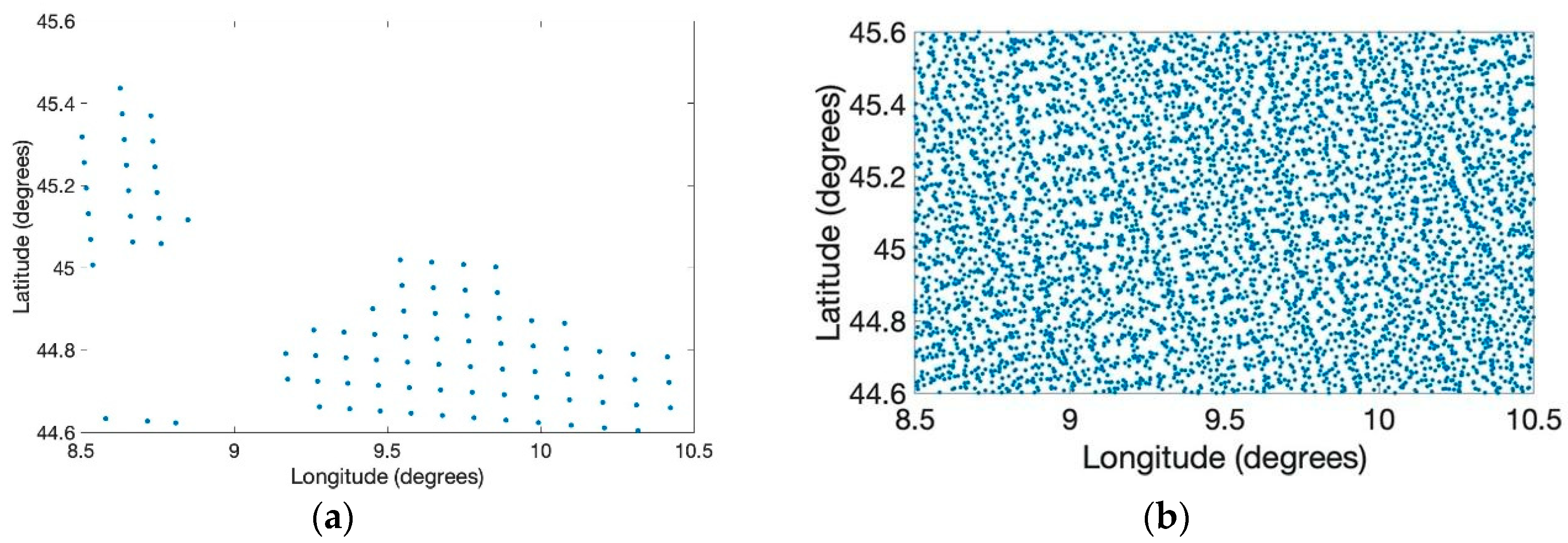
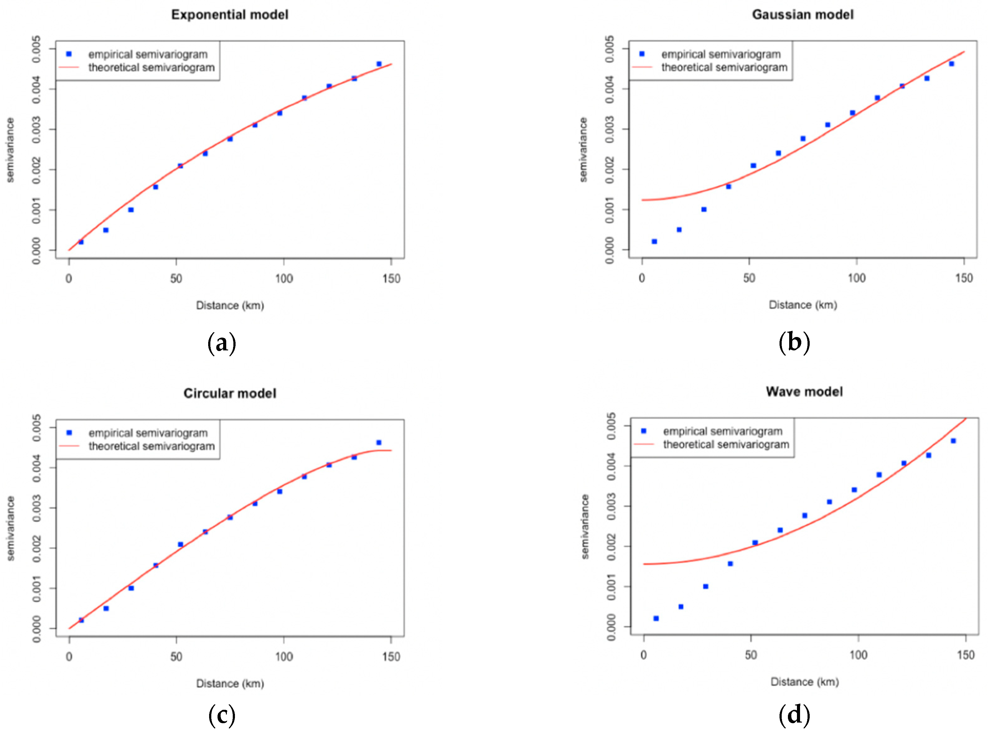
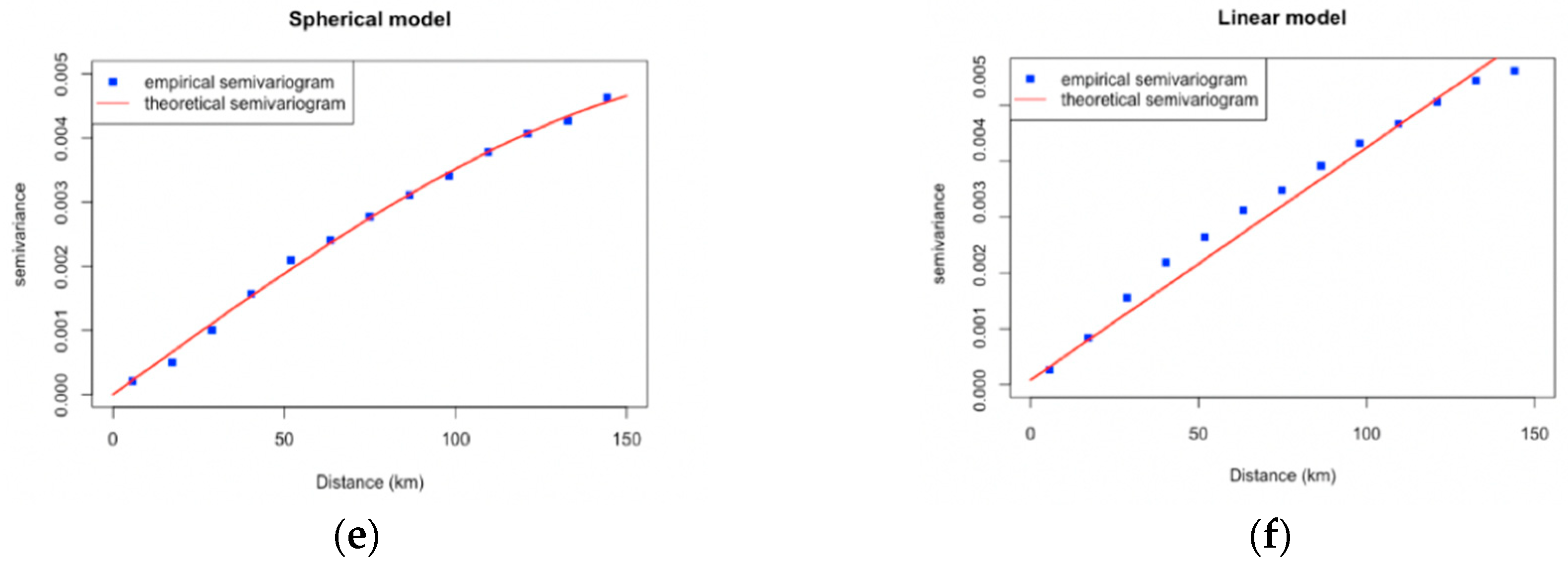
2.4. Regridding Technique

This section briefly presents the ordinary kriging method used to pass from Level 2 NO₂ data at a spatial resolution of 7 km × 3.5 km to Level 3 NO₂ data at a spatial grid-resolution of 1 km × 1 km. The methodology is quite general and can be applied to any set of data.

The regridding technique, used to estimate a variable of interest at a given spatial location, is based on the spatial autocorrelation of data [46].

Let $Z\left(s\right)$ be a spatial process, whose values or realizations are known at a set of spatial locations, say, $s=\left\{s_1,\dots ,s_n\right\}$, where $s_j$ denotes the spatial coordinate, e.g., (longitude, latitude) in a case of 2-D process. Our objective is to estimate the process at a point $s_0\notin s=\left\{s_1,\dots ,s_n\right\}$ for which no observation is available. The estimate, $\widehat{Z}\left(s_0\right)$ of $Z\left(s_0\right)$ is obtained according to [46]

$$\widehat{Z}\left(s_0\right)=\lambda Z\left(s\right),$$

(1)

where λ is a vector of real weights and $Z\left(s\right)$ represents the process at points where it is known. In order to have an unbiased estimate, the additional condition of weights normalized to unity is assumed, i.e.,

$${\displaystyle \sum }_{i=1}^n{\lambda }_i=1.$$

(2)

The weights must be properly determined to minimize (in the least Squares sense) the estimation of the variance and to ensure the estimator has no bias. In practice, the weights are determined based on the correlation properties of the process $Z\left(s\right)$. These properties are described through a functional, called semivariogram, which yields the variance of the differences between pairs of the variable under study at two different sites $s_i$ and $s_j$ [46,47]. The semivariogram is defined according to:

$$\gamma \left(s_i,s_j\right)=\frac{Var\left(Z\left(s_i\right)-Z\left(s_j\right)\right)}{2}.$$

(3)

The semivariogram is a continuous function in the origin, but, in practice, it is often observed that $\gamma \left(0\right)\ne 0$. This situation is known as nugget effect ($\gamma \left(0\right)={\tau }^2$ is called nugget), and it is linked to measurement errors or spatial resolution issues, which in turn affect the variogram value at very small distances.

Another important feature of the semivariogram function is the sill, defined as:

$${\tau }^2+{\sigma }^2=\gamma \left(h\right)$$

(4)

where ${\sigma }^2$ is known as the partial sill (the sill minus the nugget), and $h$ is the distance between two different observations. In case the sill takes on a finite value, it means that the stochastic process is weakly stationary; also, if this occurs for a finite value of $h=h^{*}$, then $h^{*}$ is said the range of the variogram. The range quantifies the distance over which two different observations can be considered correlated.

Based on the available data we can build up an empirical semivariogram, say $\widehat{\gamma }.$ In doing so, a fitting model must be considered to extrapolate the spatial behavior of the observed points to the area of interest. In the literature, there are several theoretical semivariogram models (e.g., linear, exponential, Gaussian, wave and circular), with known analytical properties and physical meaning of parameters.

In our methodology, we use a set of models, which are specified in Figure 3, and that which is best suited to our particular process $Z\left(s\right)$ is chosen based on a statistical criterion, which selects the model that best fits the given data.

In this work, the fit criterion described in [48] has been used. This step of the analysis is again exemplified in Figure 4, where for the case shown, the best model is that spherical. It has to be stressed that the fit criterion procedure is applied to case-by-case, which means that for the analysis, we are going to show it has been applied to any single, individual, monthly maps.

Once, the semivariogram model has been selected, the weights $\lambda$ can be calculated and used for the spatial interpolation.

Finally, before finishing this section, it is also worth noting that the ordinary kriging methodology is a particular case of optimal interpolation and can be looked at as a special implementation of the most general formalism of Kalman filter (e.g., see [49,50,51,52]). This is important because, unlike ad-hoc interpolation methods, the kriging provides a robust and optimal tool for interpolation processes.

3. Results

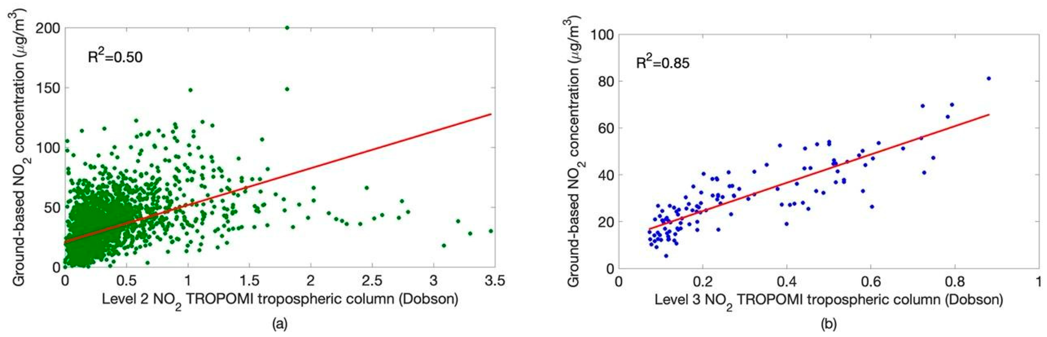
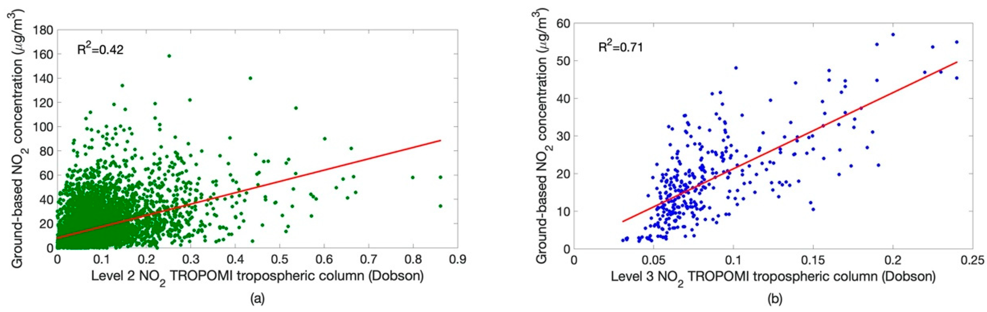
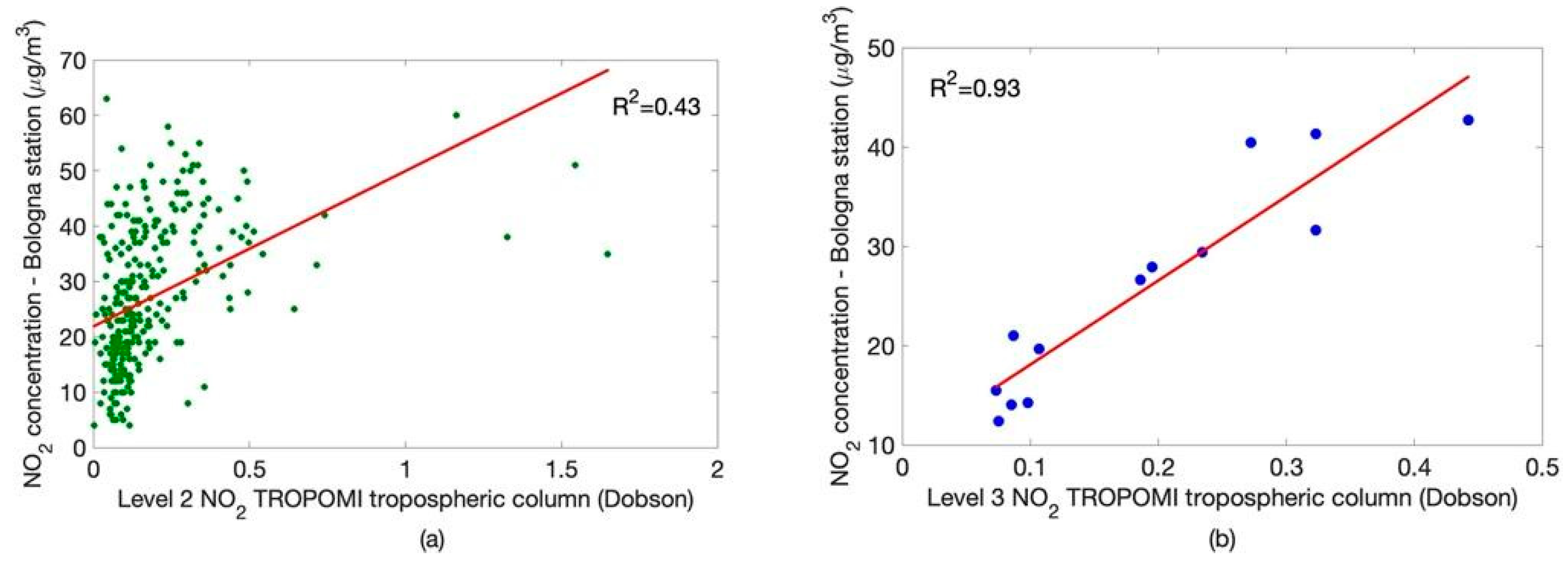
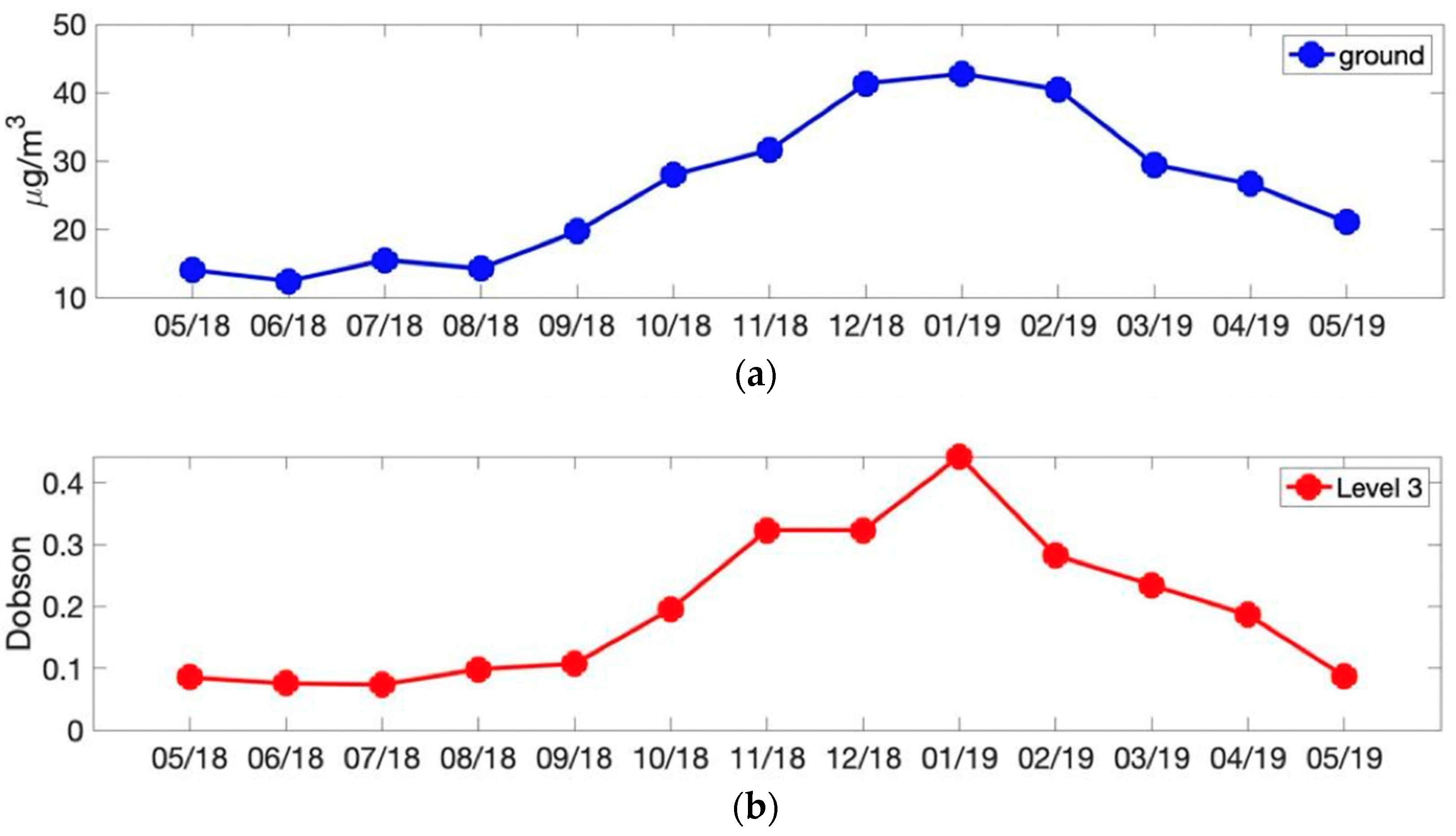
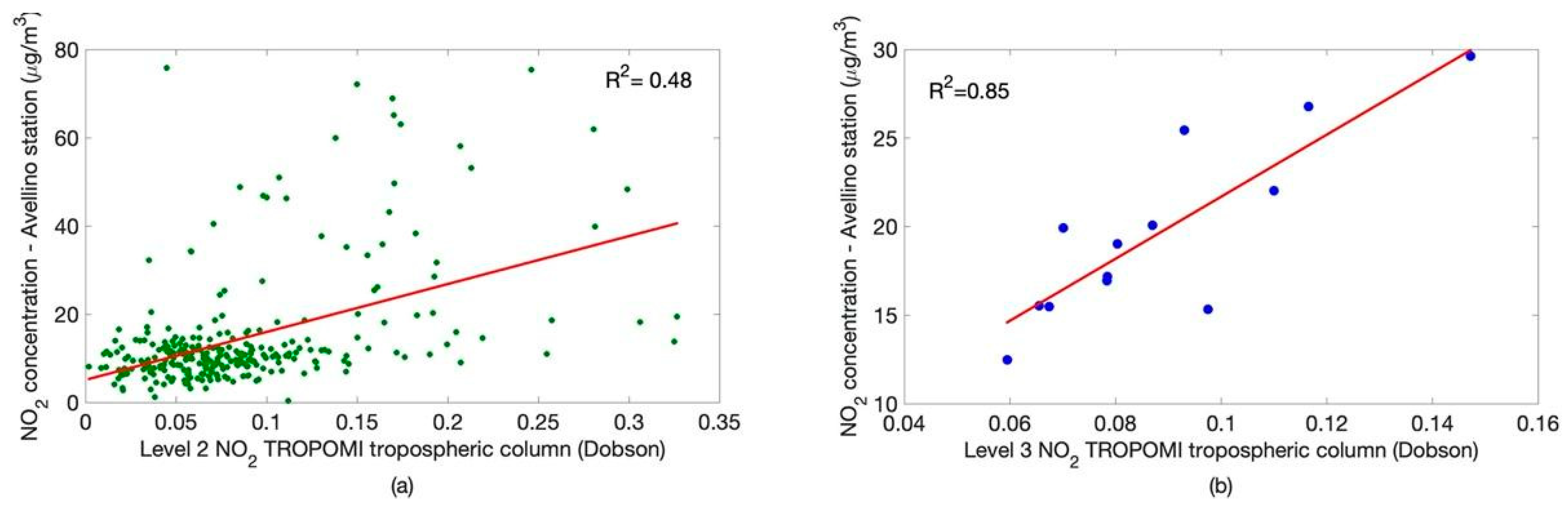
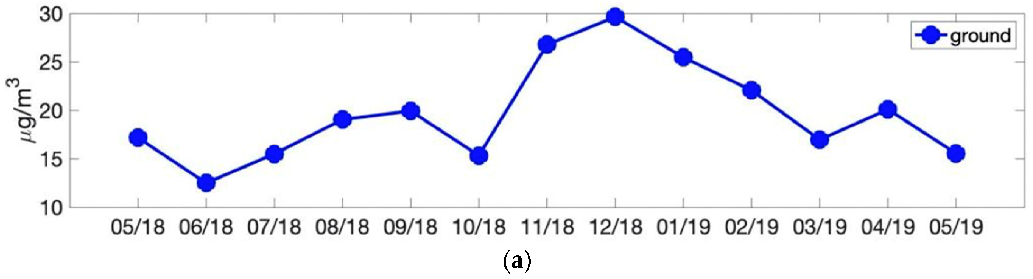
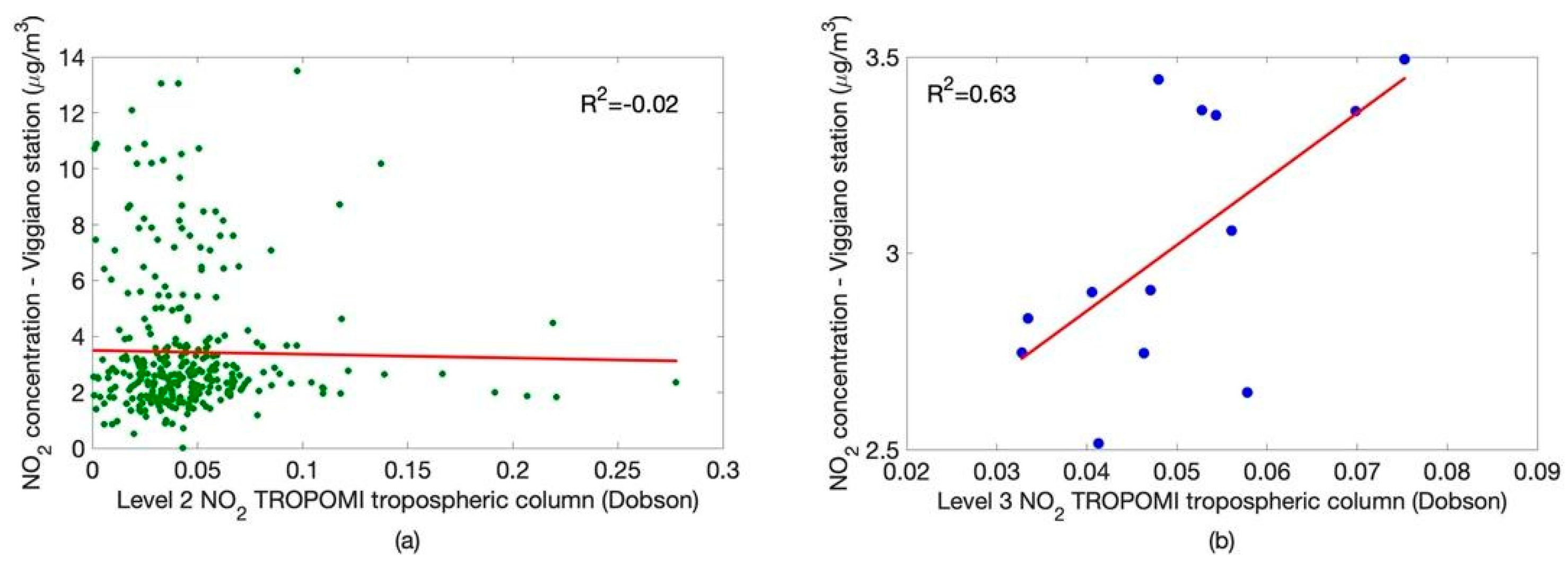
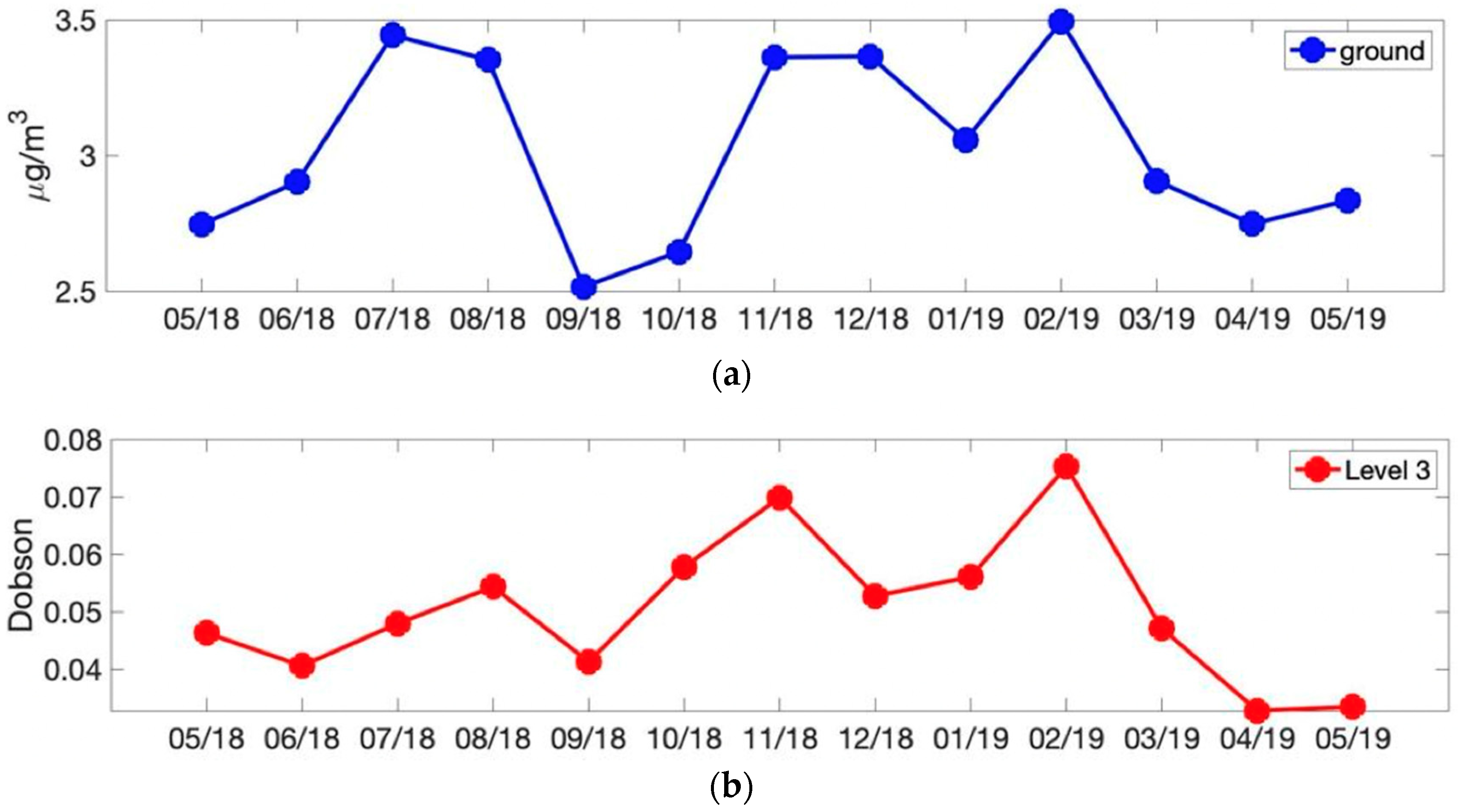
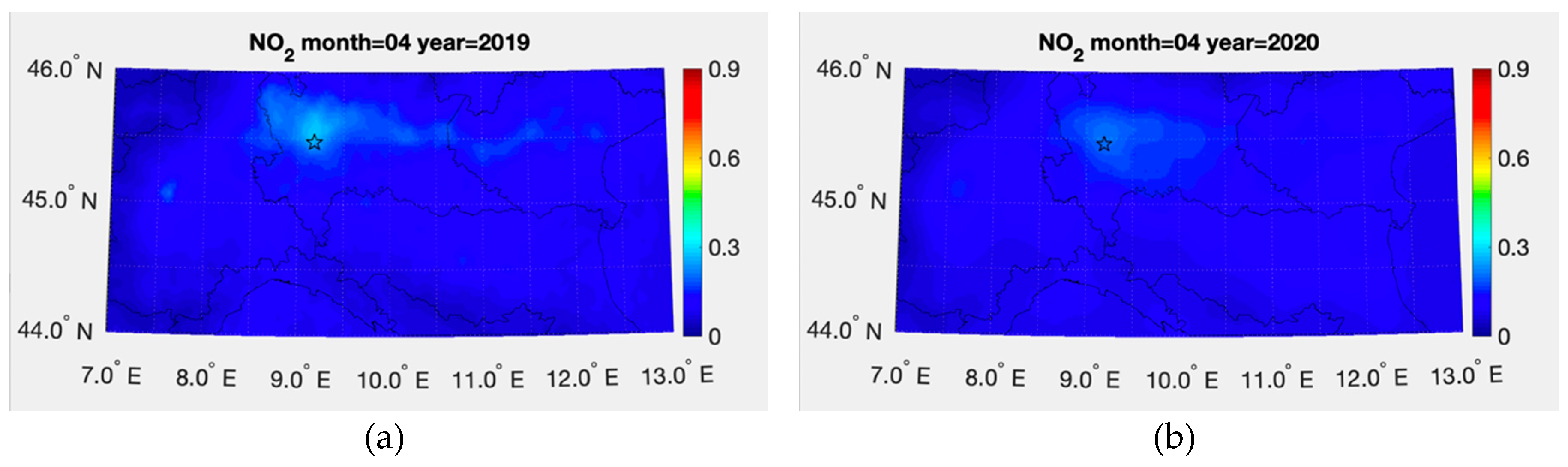
3.1. Comparing Satellite Data to in Situ Observations

In this section, we will compare in situ observations against Level 2 and Level 3 (krigged data). The final aim is to show that krigged data perform better as far as the correlation with ground-based observations is concerned.

The comparison between satellite data to in situ observations required the space-time colocation of data from the different sources. In particular, each in situ data have been compared with the spatially closest Level 2 and Level 3 TROPOMI value. About temporal colocation, each Level 2 TROPOMI observation is associated with the time of the satellite overpass, and therefore we used the temporally closest in situ measurement.

Toward this objective, the effects of the kriging procedure on Level 2 data is exemplified in Figure 5, which shows the scatterplot of time-space collocated values of TROPOMI NO₂ and in situ measurements for the ten validation stations in North Italy (see Figure 1) before and after the kriging operation. In Figure 5a, the scatterplot refers to the observations accumulated over a month but not averaged or regridded, therefore they are instantaneous measurements. After the kriging operation, Figure 5b, the data are resampled monthly at the spatial sampling of 1 km $\times$ 1 km. It is seen that the linear correlation coefficient increases from 0.50 to 0.85.

From Figure 5, we see a good linear relationship extends over the range 10–80 $\frac{\mathsf{\mu }\mathrm{g}}{{\mathrm{m}}^3}$. The results are showing that the TROPOMI can sense down to the surface and satellite data are capable of discriminating between low and high pollution load. Furthermore, Level 3 TROPOMI has a far better correlation with in situ observations. In passing, the good relationship we see for this case study shows the relatively high homogeneity of the 10 stations. In effect, they are within the bulk area of the Po Valley, which is affected by more intense and persistent air pollution concerning other regions in Italy.

Figure 6 shows the results for the 37 validation stations in Southern Italy. In comparison to Figure 5, the correlation coefficient is smaller for both Level 2 and Level 3 data, but, as before, it increases passing form the Level 2 to 3. The smaller correlation is expected because, unlike the Po Valley target area, that in Southern Italy has a much more complex orography, and is much less homogeneous as far as the air quality conditions. The target area includes large urban areas, such as the city of Naples and countryside, sparsely populated towns, which results in very large variability of air pollution intensity.

At a different degree, the results in Figure 5 and Figure 6 show that the kriging technique is capable of improving the spatial sampling and yields a better comparison with in situ observations. However, the results apply to the whole target area. In contrast, it would be better to check the capability of TROPOMI to resolve air pollution at the scale of the single station.

Towards this objective, we now come to compare satellite vs. in situ observations at every single station. For the Po Valley, the results are summarized in

Table 1. Longitude (deg east) and latitude (deg north) of North Italy ground stations, slope (parameter a in units of $\mathsf{\mu }\mathrm{g} {\mathrm{m}}^{-3} \mathrm{D}\mathrm{o}\mathrm{b}\mathrm{s}\mathrm{o}{\mathrm{n}}^{-1}$) and intercept (parameter b in units of $\mathsf{\mu }\mathrm{g} {\mathrm{m}}^{-3}$ of the linear regression, regression error (parameter e in $\mathsf{\mu }\mathrm{g} {\mathrm{m}}^{-3}$) and correlation (R²).

Ground Station	Longitude	Latitude	a	b	e	R2
BOLOGNA-DE AMICIS	11.72	44.36	84.67	9.61	3.75	0.93
BRESCIA	10.22	45.54	42.13	18.34	4.25	0.88
CITTADELLA	10.33	44.79	48.63	8.37	4.81	0.85
GIORDANI-FARNESE	9.69	45.05	57.61	16.80	5.08	0.89
MANTOVA	10.79	45.16	59.71	7.74	8.42	0.76
MILANO	9.20	45.46	42.11	25.05	7.24	0.80
PAVIA	9.15	45.18	55.83	10.95	7.68	0.83
SAN ROCCO	10.66	44.87	36.05	7.28	4.03	0.83
SESTO S. GIOVANNI	9.25	45.53	55.69	18.37	9.42	0.83
VIGEVANO	8.85	45.32	44.69	8.34	5.85	0.84

, where the correlation between TROPOMI Level 3 and in situ observations is shown. In general, we have found that the correlation improves when we move from Level 2 to Level 3, as exemplified for one of the ten stations listed in Tab. 1, in Figure 7, which shows the results for the Bologna-De Amicis station. The station is located within an urban area densely populated and with intense traffic all year-round. As said, we observe a poor correlation with Level 2 data. Conversely, we observe a very high correlation, which reaches the value of $R^2=0.93$ when going to Level 3 data. The same good correlation is also seen when we consider monthly time series as done in Figure 8. It is seen that the krigged data are capable to follow the seasonal cycle, showing an increase of NO₂ pollution in wintertime months because of the combined effect of domestic heating and increased traffic.

Overall, the good correlation we have found for the Po Valley is an effect of the better spatial sampling of L3 data, but we think it is also a consequence of the particular, local, weather conditions, which govern air circulation over the valley. The Po river flows in a closed valley surrounded by high mountains, which makes pollution remains trapped, especially in wintertime, when atmospheric conditions prevent dispersal.

TROPOMI data, as well as satellite observations, estimate tropospheric NO₂ columns rather than ground-level NO₂ concentrations, which, in turn, is normally measured from in situ stations. In addition, satellite data cannot resolve the diurnal cycle because of the polar orbits. The good correlation we observe means that, because of the huge pollution stain over the Po Valley, NO₂ tends to be compressed and trapped within the PBL. We have a persistent phenomenon, which can be measured by satellite on consecutive days. The air pollution persistence is an effect peculiar to the Po Valley and its local weather.

Other Italian regions can have local weather conditions, which can favor the dispersal of pollution. The complex orography of most of the Italian territory can impact on the PBL dynamics. As a result, we can observe vertical and horizontal inhomogeneities of NO₂ mixing ratio profiles.

In effect,

Table 2. As Table 1, but for the South Italy ground stations.

Ground Station	Longitude	Latitude	a	b	e	R2
ACERRA SCUOLA CAPORALE	14.37	40.94	248.78	−7.41	8.65	0.64
ALTAMURA	16.56	40.83	322.97	−0.69	4.16	0.75
ANDRIA	16.30	41.23	329.19	−3.15	3.33	0.84
AVELLINO	14.78	40.92	175.17	4.17	2.57	0.85
BARI-CALDAROLA	16.88	41.11	450.14	3.15	4.60	0.79
BARI-CARBONARA	16.86	41.07	302.81	−8.49	2.87	0.78
BARI-CAVOUR	16.87	41.12	229.15	17.51	3.17	0.70
BARI-CUS	16.84	41.13	236.72	−2.81	3.36	0.68
BARI-VIA KENNEDY	16.86	41.09	309.28	−0.73	2.16	0.87
BARLETTA	16.28	41.31	267.84	−3.97	2.97	0.83
BENEVENTO	14.78	41.11	716.20	−35.83	4.12	0.90
BRINDISI-VIA CRATI	17.95	40.63	226.60	1.32	1.26	0.74
CAMPI SALENTINA	18.03	40.40	321.67	−10.66	2.34	0.59
FOGGIA-VIA ROSATI	15.55	41.45	292.48	−4.51	4.50	0.68
FRANCAVILLA	17.58	40.53	337.60	−7.88	5.29	0.59
GROTTAGLIE	17.42	40.54	179.05	−4.62	2.49	0.61
LECCE-VIA GARIGLIANO	18.17	40.36	627.30	−24.79	4.00	0.55
MADDALONI	14.37	41.04	156.80	2.63	3.42	0.72
MANFREDONIA	15.91	41.63	174.43	8.44	1.59	0.90
MESAGNE	17.81	40.56	259.81	−7.18	1.71	0.74
MODUGNO-ENO2	16.77	41.14	249.02	1.21	1.92	0.87
MODUGNO-ENO3	16.78	41.09	169.26	8.88	1.36	0.83
MODUGNO-ENO4	16.79	41.11	465.30	−11.35	3.47	0.86
MOLFETTA-VERDI	16.60	41.20	297.01	−0.73	2.54	0.89
MONOPOLI-ALDO MORO	17.29	40.95	461.40	−9.14	3.97	0.81
MONOPOLI-ITALGREEN	17.28	40.96	233.88	−2.77	1.53	0.88
MONTE S. ANGELO	15.94	41.66	85.03	1.53	1.65	0.68
NAPOLI PARCO VIRGILIANO	14.18	40.79	64.97	3.87	2.34	0.67
NOCERA INFERIORE	14.64	40.74	267.29	−4.12	10.24	0.52
PORTICI	14.34	40.81	69.06	9.11	3.57	0.76
SALERNO	14.77	40.69	204.27	27.50	7.00	0.60
S. PANCRAZIO SALENTINO	17.84	40.42	164.45	−3.11	2.25	0.54
SAN SEVERO	15.38	41.69	186.92	−2.46	2.43	0.80
SURBO	18.12	40.41	257.69	−5.14	1.82	0.55
TORRE ANNUNZIATA	14.43	40.76	77.32	11.18	3.14	0.76
VIGGIANO-COSTA MOLINA	15.95	40.32	16.80	2.18	0.25	0.63
VIGGIANO 1	15.90	40.33	85.07	−0.71	1.03	0.71

(South Italy) shows a picture much more complex. In general, higher correlations are found for densely populated cities on the East coast (Adriatic Sea) and inner part (mountains). However, there is not a clear pattern. As a result of the above discussion, the cases of fair correlation ($\approx 0.50)$ could be related to the particular orography of the given area, which could influence the local weather and climate. As an example, for the city of Naples, which we know is an area of intense air pollution, likely, the local, very complex, orography and the related weather characteristics contribute to increasing the day-to-day variability of air quality and, much important, increase the vertical and horizontal inhomogeneity of NO₂.

In general, using additional physical information, e.g., see [53], the correlation could also be improved for stations showing smaller consistency between the tropospheric column and near-surface measurements. However, this is a task not addressed in this paper, which rather focuses on the direct use of TROPOMI observations per se. Nevertheless, it is fair to recall and caution the reader that the TROPOMI observes NO₂ columns rather than ground-level NO₂ concentrations, which are closely related to potentially harmful effects on human health.

Before closing this section, we stress that also for the second target area, we have that, in general, the correlation improves when we go from Level 2 to Level 3. This is exemplified for two stations in Figure 9, Figure 10, Figure 11 and Figure 12. The first station refers to the urban area of the Avellino city in the mountains. Figure 9 shows that the correlation clearly improves after the kriging applications to the Level 2 data.

The good correlation (Level 3) is also reflected in Figure 10, where we show the comparison between monthly time series. TROPOMI data are capable of following and reproduce the annual cycle, with the winter peak due to domestic heating.

Figure 11 shows the scatter plot for the second station, which is the Viggiano-Costa Molina station. This station is located in a countryside area some km apart from an oil refinery plant. Still, it is far from urban areas to monitor the supposedly NOx emissions from the industrial plant.

Unlike the former Avellino station, now the correlation coefficient goes to zero in the case of Level 2 data. For this station, we observe no sign of important pollution, as it can be argued by comparing Figure 11 to Figure 9. Nevertheless, when we pass to Level 3 data, it is seen that TROPOMI is still sensitive to these very low values of NO₂ concentrations. According to the present Italian regulation the NO₂ annual average should not exceed 40 $\frac{\mathsf{\mu }\mathrm{g}}{{\mathrm{m}}^3}$. The monthly averages for Viggiano are smaller by a factor of ten.

Although relatively small, the correlation found for the Level 3 data is still large enough to correctly reproduce the salient features of the seasonal cycle, as shown in Figure 12.

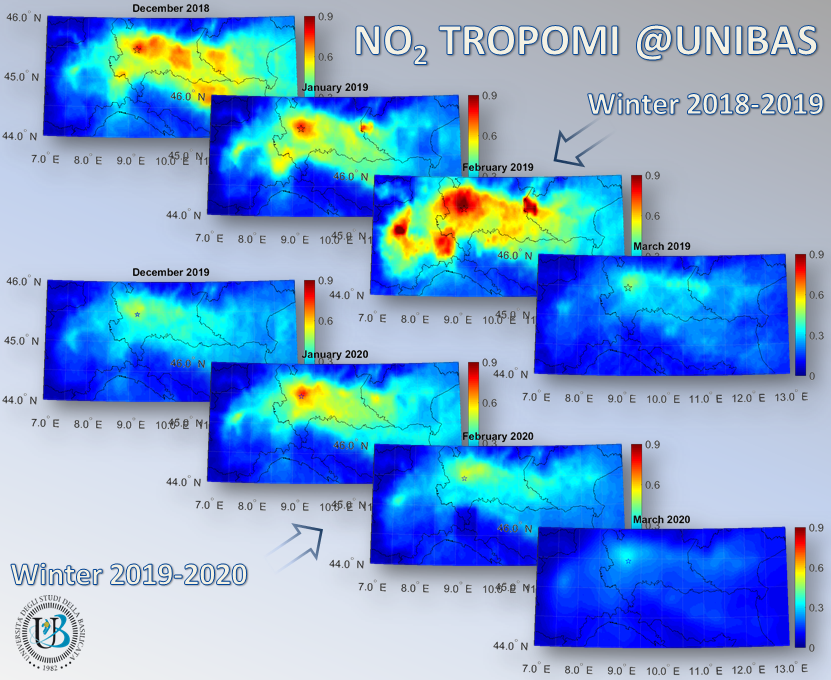
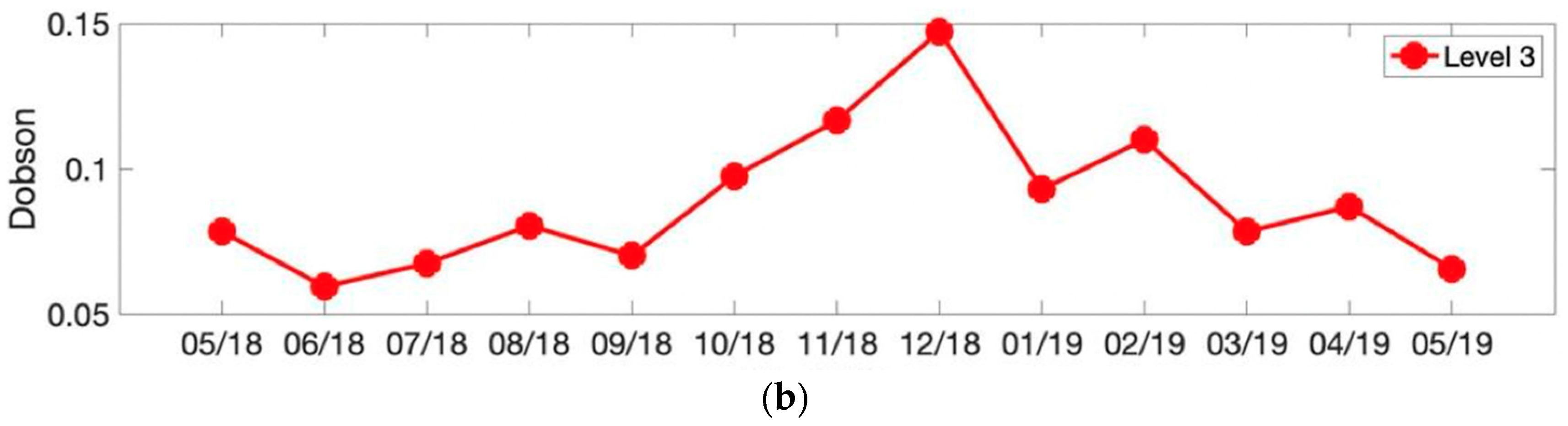
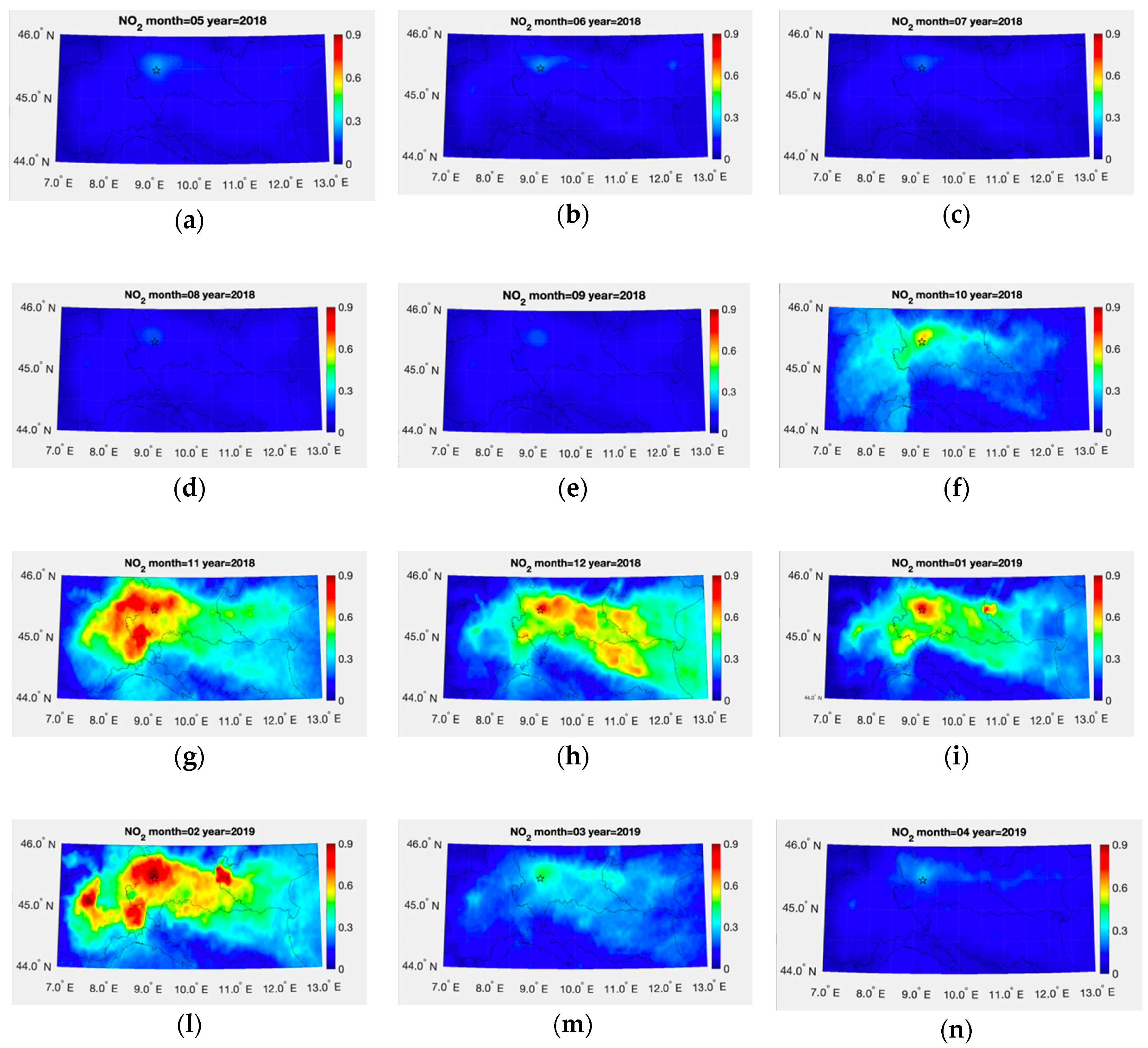
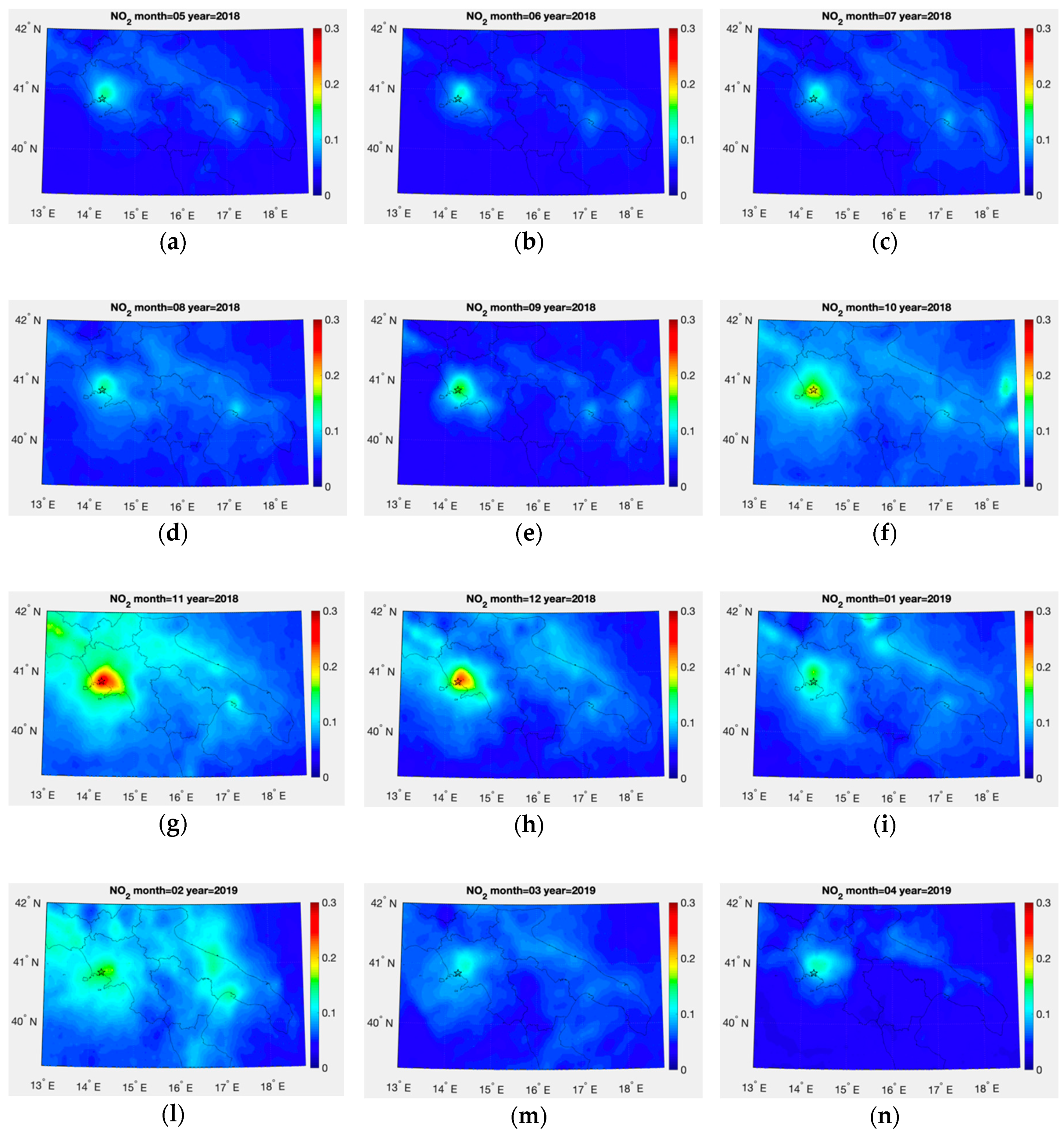
3.2. Monthly Spatial Map of Level 3 NO₂ Tropospheric Column

With the exceptions and cautions outlined above, the previous section gives us the confidence of the good reliability of TROPOMI, especially for the Po Valley, to follow the lower tropospheric column amount of NO₂ and related evolution and variations. We now pass to illustrate and describe spatial patterns of NO₂ tropospheric column data, as revealed from the TROPOMI instrument.

To begin with, Figure 13 illustrates the monthly NO₂ distribution over the Po Valley area, for the period between May 2018 to April 2019. These maps show persistent NO₂ hotspots over big cities, such as Milano (star symbol), and widespread NO₂ distribution in the colder months, particularly from November 2018 to February 2019, with peaks three times larger than those reached in the months of May-August 2018 and April 2019. This situation underlines the fact that NO₂ concentrations are strictly related to a more massive vehicular traffic (because of school season) and domestic heating, and in addition to less sunlight and colder temperatures, typical of the winter months.

Figure 14 illustrates the monthly maps of Level 3 NO₂ tropospheric column data related to the study area in the South of Italy. These maps show a persistent NO₂ hotspot in correspondence to the city of Naples (star symbol). Moreover, also for this case, we see a seasonal cycle, with a higher level of NO₂ during the months from October 2018 to February 2019. The comparison between the two target areas (North and South) shows that the densely populated and heavily industrialized Po Valley is affected by larger spatial patterns of NO₂, with concentration peaks three times larger than those reached in the Southern area.

As said before, the main reasons for the huge pollution stain over the Po Valley are closely connected to intense urban and industrial activities and to orographic aspects, which can determine unfavorable local weather conditions, which make pollution remain trapped, especially in wintertime, and prevent dispersal.

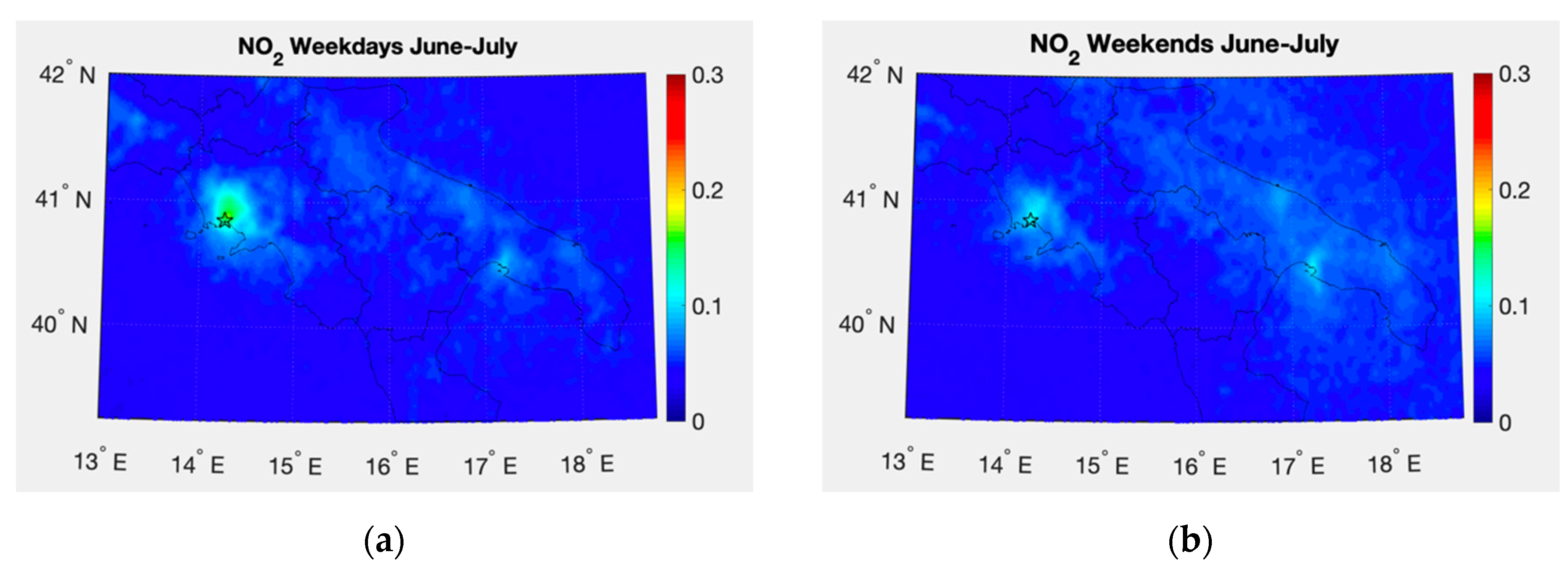
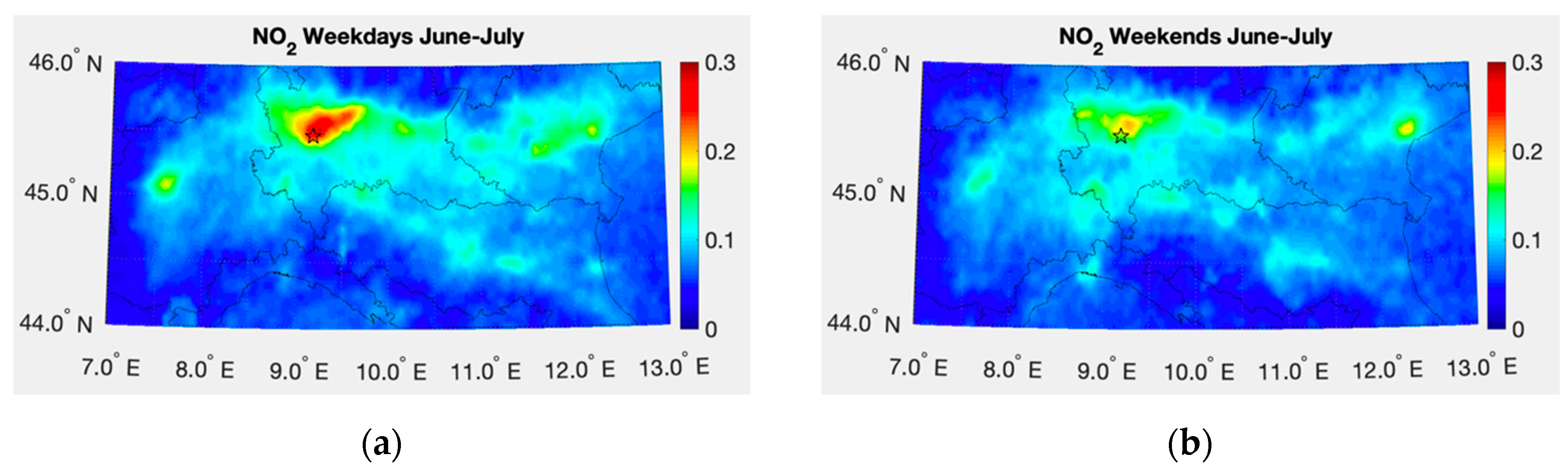
3.3. Weekdays and Weekend Observations

To show the capability of the Level 3 data to detect air quality behavior because of anthropic cyclic activities, in this section, we examine NO₂ load on weekdays and weekend times.

The analysis of weekly cycles captures lower NO₂ levels during the weekend days compared to the weekdays, as a result of reduced emissions from traffic and industrial activities, which are more intense in urban areas. Differently to previous work [29], we only used two days for weekdays and not all five days from Monday to Friday to have uniformity with the two days of the weekend.

More in detail, 16 weekdays (Wednesday and Thursday) and 16 weekend days for June and July were considered for the two target areas. The analysis has been performed in summer so that the results are not affected by domestic heating. The results are shown in Figure 15 (Southern Italy) and Figure 16 (Po Valley), and for both cases, it is possible to note the higher NO₂ concentrations over urban districts, such as Naples and Milan.

In passing, we draw attention to a striking feature, which can be seen in Figure 16a. If we draw the diagonal from top left to bottom right, it is seen that the NO₂ pollution tends to be higher along that direction, from the bottom right to the middle of the map. In effect, that is the main direction of the heavily trafficked Italian A1 highway.

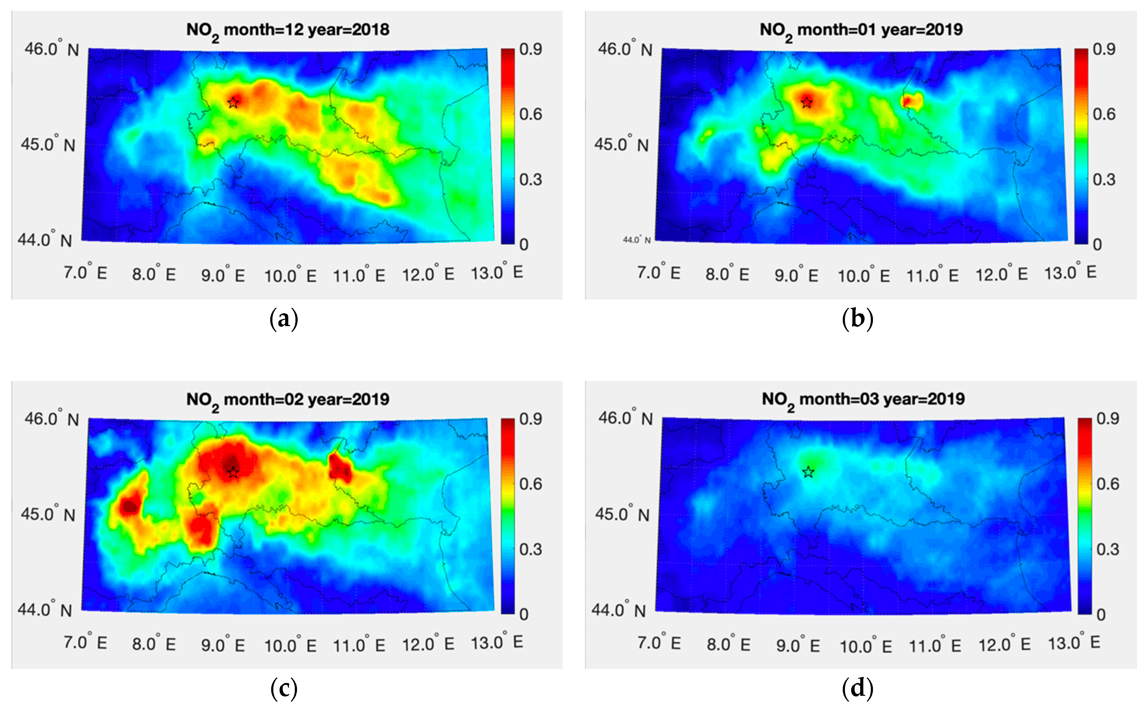
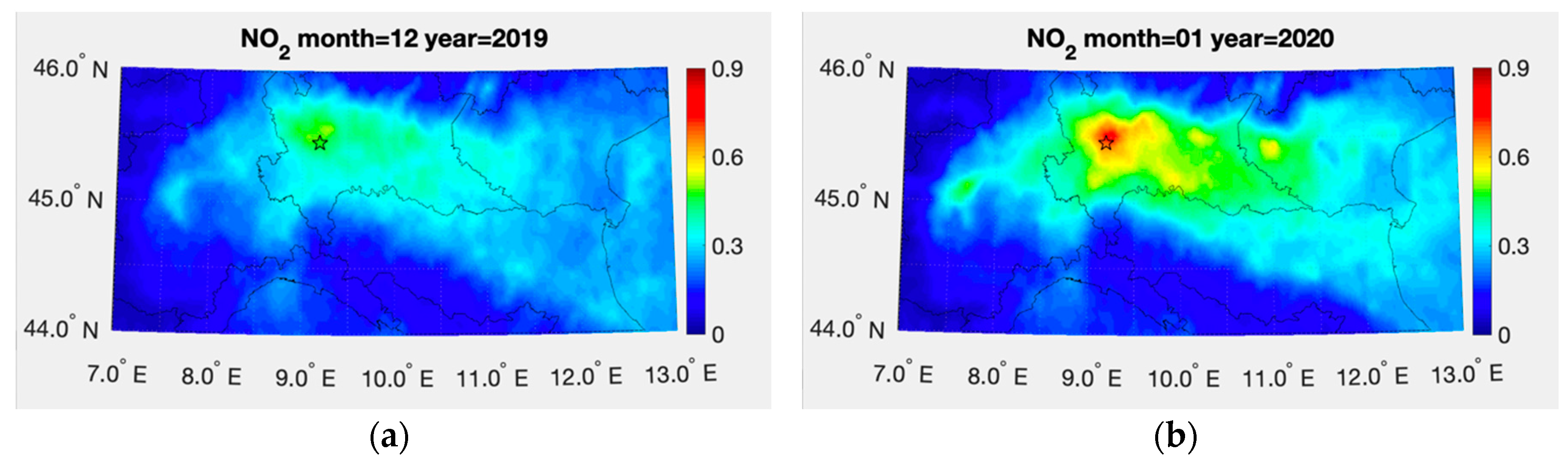
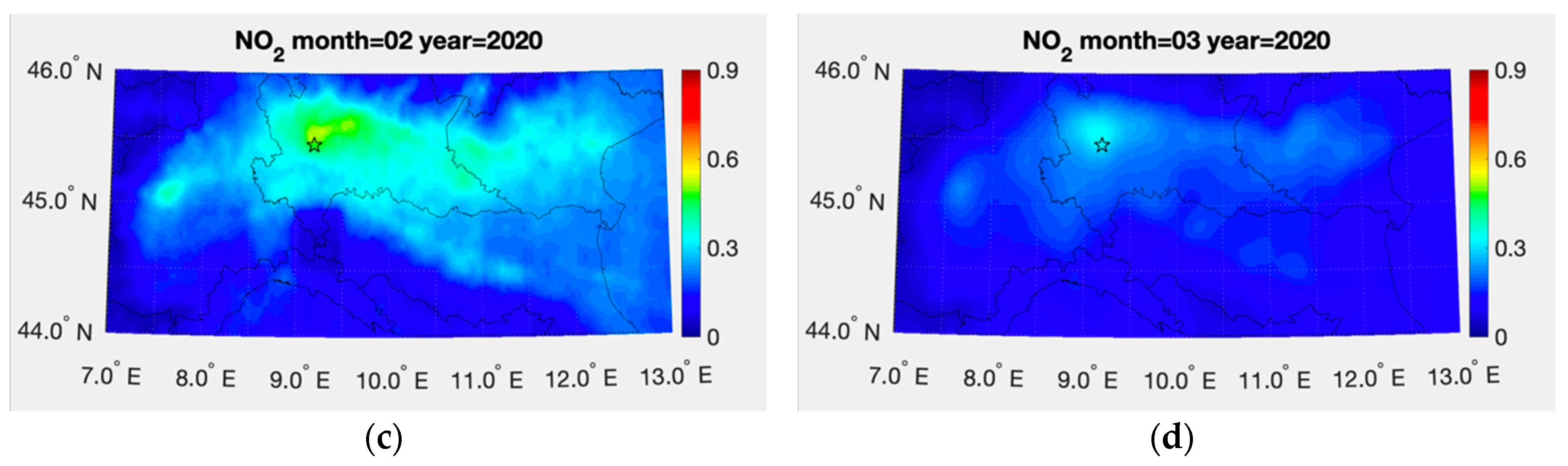
3.4. NO₂ Pollution During COVID-19 Epidemic Crisis

While writing this paper, Italy has been hit by the dramatic COVID-19 epidemic. As a result that the science community has drawn attention to the possible interrelationship between COVID-19 diffusion and air quality, we have assessed the evolution of NO₂ pollution over the Po Valley in the period Dec. 2019 to Apr. 2020. In this period, COVID-19 has spread and supposedly infected millions of people, leading Italian authorities to declare the lockdown of the Po Valley area, which has been later extended to the whole Nation. We stress that we just put attention on the NO₂ evolution per se; in other words, we just show how this evolution has been observed and photographed from space.

For a proper comparison, the monthly maps of NO₂ concentration over the Po Valley for the period December to March for both the COVID-19 (that is 2019–2020) and the no COVID (2018–2019) periods are shown in Figure 17 and Figure 18, respectively. The first striking feature which arises from the comparison of the corresponding maps for no-COVID-19 (Figure 17) and COVID-19 (Figure 18) is the sharp decrease of air pollution in 2020 compared to 2019. This has been most likely the effect of the warmer 2019-20 winter, which has limited the use of heating power for both residential and commercial sectors. It is to be stressed that according to ECMWF, winter 2020 has been the far warmest winter season ever recorded over Europe (e.g., see https://climate.copernicus.eu/boreal-winter-season-1920-was-far-warmest-winter-season-ever-recorded-europe-0).

By comparing Figure 17 to Figure 18, we see that only January 2019 and 2020 show comparable NO₂ pollution, whereas February 2020 shows a dramatic decrease of NO₂ pollution over the whole Po Valley. This month has been supposedly that of maximum virus diffusion among the population.

In March 2020, when the lockdown was active, we see some 50% decrease of NO₂ pollution concerning the same month of 2019. The same situation also occurs for April, which is shown in Figure 19.

To sum up, we can say that during the lockdown, NO₂ has decreased over the Po Valley. However, this decrease is over-imposed to a general decreasing trend because of the favorable 2020 weather conditions. The general reduction in NO₂ pollution during the 2020 winter is also clearly seen at ground stations and therefore is not an artifact of satellite data. This is exemplified in

Table 3. Monthly percentage variations of NO₂ concentrations for the month December 2019–April 2020 to December 2018–April 2019, as measured by TROPOMI Level 3 data and in situ stations.

	Bergamo		Brescia		Milano
Month	Satellite	In Situ	Satellite	In Situ	Satellite	In Situ
December	−39.3%	−37.4%	−30.5%	−16.0%	−29.4%	−25.6%
January	−9.4%	−14.2%	−10.6%	−9.0%	−5.0%	−26.08%
February	−28.1%	−44.4%	−33.3%	−23.9%	−39.2%	−18.47%
March	−25.8%	−49.2%	−44.7%	−41.12%	−21%	−33.85%
April	−20.0%	−30.1%	−15.8%	−51.8%	−16.7%	−40.0%

, which shows the percentage variation among 2019 and 2020 winter months as measured at ground stations in Bergamo, Brescia and Milan, respectively. These three cities are those who share the bulk of NO₂ concentrations over the Po Valley. Furthermore, the negative variations are confirmed with TROPOMI data, as can be directly checked by the same Table 3.

4. Discussion

Kriging and related tools are now of widespread use within the context of Geostatistics and the analysis of Geospatial data (e.g., [54,55,56]). Application to the particular area of air quality with a focus on NO₂ has been recently reported in the literature [57,58], which emphasizes the use of in situ observations. Our application to TROPOMI is quite new, and it has been designed to improve the spatial sampling of the data, which is inevitably affected by gaps because of cloudy conditions. In fact, we use a mosaic of TROPOMI overpasses, which is used to estimate the semivariogram that governs the data structure at the different spatial scales. Once we have estimated the semivariogram, we perform a regridding of the data on a finer, regular, grid mesh with a step $∆r=$1 km. The regridding fills the gaps in the original footprint geometry and improves the colocation with in situ observations. We stress that the step $∆r=$1 km should not be confused with the spatial resolution of the original data, which remains fixed to that of the TROPOMI footprint geometry. In fact, in our kriging procedure, there is no explicit de-convolution of the original observations or information from additional sources of data at better spatial resolution. Using regridding we oversample the original TROPOMI footprints to match the position of ground stations better and perform time-averaging of the data. It could be argued that this remapping could be performed in many different ways involving mathematical interpolation tools. The specificity of kriging methods is that they do not only consider the distance between observations, but they also capture the spatial structure in the data by computing the variogram and using it to set the weights to perform the interpolation at un-sampled points in the grid. To show the kriging advantages, we have also produced NO₂ maps for the Po Valley using the technique of the nearest neighbor combined with the ordinary arithmetic mean. In doing so, Level 2 data were accumulated for each month on a regular, fixed, grid which has the size of the TROPOMI original spatial resolution of 7 km × 3.5 km. For each satellite overpass, the nodes of this regular grid were filled with the spatially closest Level 2 value (within a maximum distance that refers to the original Level 2 TROPOMI spatial resolution) and, subsequently, the regularly spatially distributed values were averaged over the month. In this way, we can obtain at each node a value which is representative of the monthly averaged Level 2 NO₂ TROPOMI tropospheric column. The results are shown in Figure 20 for the station of Bologna, so that they can be directly compared to those of Figure 7. It is seen that we improve the correlation with respect to Level 2 data, but not concerning kriging for which we observe a correlation of 0.93 against that of 0.80 shown in Figure 20.

Another important aspect to discuss is that regarding the choice of the grid step $∆r=$1 km. Although there is no general prescription on how to choose the grid step, the case study at hand is normally suggesting a suitable pragmatic and effective choice. It is normally suggested (see e.g., [56], section 5.4.2) that $∆r"h^{*}$ ($h^{*}$ is the range that for our analysis is of the order of 100 km, e.g., see Figure 3) and that the number of couples in any grid-box should range between 6-24 (see e.g., [55], Section 5.4.2). In addition, for our application, it is obvious to require $∆r$ to be smaller than the average radius of the TROPOMI footprint. Otherwise, as shown in Figure 20, we could not take advantage of the oversampling, which is allowed with our mosaic of monthly scenes. If we take $∆r$ larger than the TROPOMI footprint, there would be no point in oversampling since we could fill gaps with available clear sky data, if any, for the given scene. Finally, according to [55], at least 6-12 points should be used for each predicted value. In our case, with $∆r=$ 1 km we have that each grid box has $\approx 10$ neighbor pairs to be used for interpolation. In this way, for any grid point, considering the four quadrants, there are some 40 neighbors to be considered for interpolation. This density of satellite observations also ensures that we have enough points covering the time window of one month. This allows us to take into account the day-to-day variability, which is needed to have a good estimate of the monthly mean.

5. Conclusions

In this paper, a geostatistical regridding technique, i.e., the ordinary kriging, was applied to improve the spatial resolution of satellite-based NO₂ tropospheric column estimations from the original coarser resolution (7 km × 3.5 km) to a final finer grid-resolution (1 km × 1 km). The finer resolution allowed us to explore spatial data variability, obtaining more information on the main NO₂ sources.

The analysis of the consistency between satellite and ground-based NO₂ values showed good correlations that demonstrated the capability of the TROPOMI instrument to well reproduce the variability of NO₂ concentrations in the lower troposphere, especially for the Po Valley. This consistency has been tested both for the original Level 2 and for the Level 3 NO₂ data, obtaining an improvement of correlation coefficients when we move from Level 2 to 3.

In effect, once properly filtered and remapped with our kriging procedure, TROPOMI NO₂ concentration showed good consistency with in situ observations. This consistency was assessed through the calculation of the linear correlation coefficients, which reached values larger than 0.90 for severely polluted areas, such as those in the Po Valley. This is an important result in that it can allow us to use TROPOMI data in air quality protocols to check and monitor, e.g., the effect of ad hoc measures to mitigate and lower the intensity of air pollution. This could have a high impact on the European Copernicus Program and boost the use of the European satellite platform.

Having said that, we have also found, for the target area in southern Italy, much more mixed results, which are likely because of an unstable PBL, which could well condition the local weather in a way to increase the vertical and horizontal inhomogeneity of NO₂. For Southern Italy, there remain cases for which from the satellite data, we can observe pollution spots, whose magnitude and intensity cannot be easily extrapolated from the troposphere to the air close to the surface.

We have also used TROPOMI data to analyze NO₂ pollution during COVID-19 and no-COVID-19 times. We have shown that TROPOMI observations have been sensitive to the lockdown effect on air quality, showing a general decrease of NO₂ concentrations in March and April 2020. However, at the same time TROPOMI, in agreement with in situ observations, has shown a general decrease of lower tropospheric NO₂ to 2019, mostly because of a warmer 2020 winter that has limited the use of power for residential and commercial heating.

References

1. Van Geffen, J.H.G.M.; Eskes, H.J.; Boersma, K.F.; Maasakkers, J.D.; Veefkind, J.P. TROPOMI ATBD of the Total and Tropospheric NO2 Data Products; Royal Netherlands Meteorological Institute (KNMI): De Bilt, The Netherlands, 2019. [Google Scholar]
2. World Health Organization. Health Aspects of Air Pollution with Particulate Matter, Ozone and Nitrogen Dioxide; World Health Organization: Bonn, Germany, 2003. [Google Scholar]
3. Sillam, S.; Logan, J.A.; Wofsy, S.C. The sensitivity of ozone to nitrogen oxides and hydrocarbons in regional ozone episodes. J. Geophys. Res. 1990, 95, 1837–1851. [Google Scholar]
4. Fuglestvedt, J.S.; Berntsen, T.; Isaksen, I.S.A.; Mao, H.; Liang, X.Z.; Wang, W.C. Climatic forcing of nitrogen oxides through changes in tropospheric ozone and methane. Atmos. Environ. 1999, 33, 961–977. [Google Scholar] [CrossRef]
5. Shindell, D.T.; Faluvegi, G.; Koch, D.M.; Schmidt, G.A.; Unger, N.; Bauer, S.E. Improved attribution of climate forcing to emissions. Science 2009, 326, 716–718. [Google Scholar] [CrossRef] [PubMed] [Green Version]
6. Seinfeld, J.H.; Pandis, S.N. Atmospheric Chemistry and Physics—From Air Pollution to Climate Change, 2nd ed.; John Wiley & Sons: New York, NY, USA, 2006. [Google Scholar]
7. Hains, J.C.; Boersma, K.F.; Kroon, M.; Dirksen, R.J.; Cohen, R.C.; Perring, A.E.; Bucsela, E.; Volten, H.; Swart, D.P.J.; Richter, A.; et al. Testing and improving OMI DOMINO tropospheric NO2 using observations from the DANDELIONS and INTEX-B validation campaigns. J. Geophys. Res. 2010, 115, 20. [Google Scholar] [CrossRef]
8. Masieri, S.; Bortoli, D.; Petritoli, A.; Kostadinov, I.; Premuda, M.; Ravegnani, F.; Carnevale, C.; Pisoni, E.; Volta, M.; Giovanelli, G. Tropospheric profile of NO2 over the Po Valley measured with scan DOAS spectrometer. In Proceedings of the SPIE 7478, Remote Sensing for Environmental Monitoring, GIS Applications, and Geology IX, 74782I, Berlin, Germany, 7 October 2009. [Google Scholar] [CrossRef]
9. Piters, A.; Boersma, K.F.; Kroon, M.; Hains, J.C.; Roozendael, M.V.; Wittrock, F.; Abuhassan, N.; Adams, C.; Akrami, M.; Allaart, M.A.F.; et al. The Cabauw Intercomparison campaign for Nitrogen Dioxide measuring Instruments (CINDI): Design, execution, and early results. Atmos. Meas. Tech. 2012, 5, 457–485. [Google Scholar] [CrossRef] [Green Version]
10. Lorente, A.; Boersma, K.F.; Yu, H.; Dörner, S.; Hilboll, A.; Richter, A.; Liu, M.; Lamsal, L.N.; Barkley, M.; De Smedt, I.; et al. Structural uncertainty in air mass factor calculation for NO2 and HCHO satellite retrievals. Atmos. Meas. Tech. 2017, 10, 759–782. [Google Scholar] [CrossRef] [Green Version]
11. Tie, X.; Huang, R.J.; Cao, J.; Zhang, Q.; Cheng, Y.; Su, H.; Chang, D.; Pöschl, U.; Hoffmann, T.; Dusek, U.; et al. Severe Pollution in China Amplified by Atmospheric Moisture. Sci. Rep. 2017, 7, 15760. [Google Scholar] [CrossRef]
12. Lamsal, L.N.; Janz, S.J.; Krotkov, N.A.; Pickering, K.E.; Spurr, R.J.D.; Kowalewski, M.G.; Loughner, C.P.; Crawford, J.H.; Swartz, W.H.; Herman, J.R. High-resolution NO2 observations from the Airborne Compact Atmospheric Mapper: Retrieval and validation. J. Geophys. Res. Atmos. 2017, 122, 1953–1970. [Google Scholar] [CrossRef]
13. Su, T.; Li, Z.; Kahn, R. Relationships between the planetary boundary layer height and surface pollutants derived from lidar observations over China: Regional pattern and influencing factors. Atmos. Chem. Phys. 2018, 18, 15921–15935. [Google Scholar] [CrossRef] [Green Version]
14. Schreier, S.F.; Richter, A.; Burrows, J.P. Near-surface and path-averaged mixing ratios of NO2 derived from car DOAS zenith-sky and tower DOAS off-axis measurements in Vienna: A case study. Atmos. Chem. Phys. 2019, 19, 5853–5879. [Google Scholar] [CrossRef] [Green Version]
15. Berkhout, A.J.C.; Gast, L.F.L.; van der Hoff, G.R.; Swart, D.P.J.; Hoed, M.; Allaart, M. Atmospheric NO2 profiles measured with lidar during the CINDI-2 campaign. EPJ Web Conf. 2018, 176, 10002. [Google Scholar] [CrossRef] [Green Version]
16. Wang, Y.; Dörner, S.; Donner, S.; Böhnke, S.; De Smedt, I.; Dickerson, R.R.; Dong, Z.; He, H.; Li, Z.; Li, Z.; et al. Vertical profiles of NO2, SO2, HONO, HCHO, CHOCHO and aerosols derived from MAX-DOAS measurements at a rural site in the central western North China Plain and their relation to emission sources and effects of regional transport. Atmos. Chem. Phys. 2019, 19, 5417–5449. [Google Scholar] [CrossRef] [Green Version]
17. Platt, U. Differential Optical Absorption Spectroscopy (DOAS). Air monitoring by spectroscopic techniques. Chem. Anal. 1994, 127, 27–76. [Google Scholar]
18. Burrows, J.P.; Weber, M.; Buchwitz, M.; Rozanov, V.; Ladstätter-Weißenmayer, A.; Richter, A.; Debeek, R.; Hoogen, R.; Bramstedt, K.; Eichmann, K.U.; et al. The Global Ozone Monitoring Experiment (GOME): Mission concept and first results. J. Atmos. Sci. 1999, 56, 151–175. [Google Scholar] [CrossRef]
19. Bovensmann, H.; Burrows, J.P.; Buchwitz, M.; Frerick, J.; Noel, S.; Rozanov, V.V.; Chance, K.V.; Goede, A.P.H. SCIAMACHY: Mission objectives and measurement modes. J. Atmos. Sci. 1999, 56, 127–150. [Google Scholar] [CrossRef] [Green Version]
20. Levelt, P.F.; van den Oord, G.H.J.; Dobber, M.R.; Malkki, A.; Visser, H.; de Vries, J.; Stammes, P.; Lundell, J.O.V.; Saari, H. The Ozone Monitoring Instrument. IEEE Trans. Geosci. Remote Sens. 2006, 44, 1093–1101. [Google Scholar] [CrossRef]
21. Munro, R.; Eisinger, M.; Anderson, C.; Callies, J.; Corpaccioli, E.; Lang, R.; Lefebvre, A.; Livschitz, Y.; Albinana, A.P. GOME-2 on MetOp. In Proceedings of the 2006 EUMETSAT Meteorological Satellite Conference, Helsinki, Finland, 12–16 June 2006. [Google Scholar]
22. Veefkind, J.P.; Aben, I.; McMullan, K.; Förster, H.; De Vries, J.; Otter, G.; Claas, J.; Eskes, H.J.; De Haan, J.F.; Kleipool, Q.; et al. TROPOMI on the ESA Sentinel-5 Precursor: A GMES mission for global observations of the atmospheric composition for climate, air quality and ozone layer applications. Remote Sens. Environ. 2012, 120, 70–83. [Google Scholar] [CrossRef]
23. Kim, H.C.; Lee, P.; Judd, L.; Pan, L.; Lefer, B. OMI NO2 column densities over North American urban cities: The effect of satellite footprint resolution. Geosci. Model Dev. 2016, 9, 1111–1123. [Google Scholar] [CrossRef] [Green Version]
24. Lamsal, L.N.; Martin, R.V.; van Donkelaar, A.; Steinbacher, M.; Celarier, E.A.; Bucsela, E.; Dunlea, E.J.; Pinto, J.P. Ground-level nitrogen dioxide concentrations inferred from the satellite-borne Ozone Monitoring Instrument. J. Geophys. Res. 2008, 113, D16308. [Google Scholar] [CrossRef] [Green Version]
25. Novotny, E.V.; Bechle, M.J.; Millet, D.B.; Marshall, J.D. National satellite-based land-use regression: NO2 in the United States. Environ. Sci. Technol. 2011, 45, 4407–4414. [Google Scholar] [CrossRef]
26. Bechle, M.J.; Millet, D.B.; Marshall, J.D. National spatiotemporal exposure surface for NO2: Monthly scaling of a satellite-derived land-use regression. Environ. Sci. Technol. 2015, 49, 12297–12305. [Google Scholar] [CrossRef]
27. Young, M.T.; Bechle, M.J.; Sampson, P.D.; Szpiro, A.A.; Marshall, J.D.; Sheppard, L.; Kaufman, J.D. Satellite-based NO2 and model validation in a national prediction model based on universal kriging and land-use regression. Environ. Sci. Technol. 2016, 50, 3686–3694. [Google Scholar] [CrossRef] [PubMed] [Green Version]
28. Goldberg, D.L.; Lamsal, L.N.; Loughner, C.P.; Swartz, W.H.; Lu, Z.; Streets, D.G. A high-resolution and observationally constrained OMI NO2 satellite retrieval. Atmos. Chem. Phys. 2017, 17, 11403–11421. [Google Scholar] [CrossRef] [Green Version]
29. Ialongo, I.; Virta, H.; Eskes, H.; Hovila, J.; Douros, J. Comparison of TROPOMI/Sentinel 5 Precursor NO2 observations with ground-based measurements in Helsinki. Atmos. Meas. Tech. 2020, 13, 205–218. [Google Scholar] [CrossRef] [Green Version]
30. Boersma, K.F.; Jacob, D.J.; Trainic, M.; Rudich, Y.; DeSmedt, I.; Dirksen, R.; Eskes, H.J. Validation of urban NO2 concentrations and their diurnal and seasonal variations observed from the SCIAMACHY and OMI sensors using in situ surface measurements in Israeli cities. Atmos. Chem. Phys. 2009, 9, 3867–3879. [Google Scholar] [CrossRef] [Green Version]
31. De Foy, B.; Lu, Z.; Streets, D.G. Impacts of control strategies, the Great Recession and weekday variations on NO2 columns above North American cities. Atmos. Environ. 2016, 138, 74–86. [Google Scholar] [CrossRef]
32. KNMI. Algorithm Theoretical Basis Document for the TROPOMI L01b Data Processor; KNMI: De Bilt, The Netherlands, 2017. [Google Scholar]
33. Griffin, D.; Zhao, X.; McLinden, C.A.; Boersma, F.; Bourassa, A.; Dammers, E.; Degenstein, D.; Eskes, H.; Fehr, L.; Fioletov, V.; et al. High-resolution mapping of nitrogen dioxide with TROPOMI: First results and validation over the Canadian oil sands. Geophs. Res. Lett. 2019, 46, 1049–1060. [Google Scholar] [CrossRef] [Green Version]
34. Boersma, K.F.; Eskes, H.J.; Brinksma, E.J. Error analysis for tropospheric NO2 retrieval from space. J. Geophys. Res. 2004, 109, DO4311. [Google Scholar] [CrossRef]
35. Boersma, K.F.; Eskes, H.J.; Dirksen, R.J.; Van Der, A.R.J.; Veefkind, J.P.; Stammes, P.; Huijnen, V.; Kleipool, Q.L.; Sneep, M.; Claas, J.; et al. An improved tropospheric NO2 column retrieval algorithm for the Ozone Monitoring Instrument. Atmos. Meas. Tech. 2011, 4, 1905–1928. [Google Scholar] [CrossRef] [Green Version]
36. Platt, U.; Stutz, J. Differential Optical Absorption Spectroscopy: Principles and Applications; Springer: Berlin, Germany, 2008. [Google Scholar] [CrossRef] [Green Version]
37. Williams, A.P.; Cook, B.I.; Smerdon, J.E.; Bishop, D.A.; Seager, R.; Mankin, J.S. The 2016 southeastern U.S. drought: An extreme departure from centennial wetting and cooling. J. Geophys. Res. Atmos. 2017, 122, 10888–10905. [Google Scholar] [CrossRef]
38. CREODIAS Platform. Available online: https://creodias.eu (accessed on 20 May 2020).
39. ARPA Basilicata. Available online: http://www.arpab.it (accessed on 20 May 2020).
40. ARPA Campania. Available online: https://www.arpacampania.it (accessed on 20 May 2020).
41. ARPA Puglia. Available online: http://www.arpa.puglia.it (accessed on 20 May 2020).
42. ARPA Lombardia. Available online: https://www.arpalombardia.it (accessed on 20 May 2020).
43. ARPA Emilia-Romagna. Available online: https://www.arpae.it (accessed on 20 May 2020).
44. Koner, P.K.; Harris, A.R.; Dash, P. A deterministic method for profiles retrievals from hyperspectral satellite measurements. IEEE Trans. Geosci. Remote Sens. 2016, 54, 5657–5670. [Google Scholar] [CrossRef]
45. Koner, P.K.; Dash, P. Maximizing the information content of ill-posed space-based measurements using Deterministic Inverse Method. Remote Sens. 2018, 10, 994. [Google Scholar] [CrossRef] [PubMed] [Green Version]
46. Cressie, N.A.C. Statistics for Spatial Data, revised ed.; Wiley-Interscience Publication: New York, NY, USA, 2015. [Google Scholar]
47. Wackernagel, H. Multivariate Geostatistics. An Introduction with Applications; Springer: Berlin, Germany, 2003. [Google Scholar]
48. Cersosimo, A.; Larosa, S.; Romano, F.; Cimini, D.; Di Paola, F.; Gallucci, D.; Gentile, S.; Geraldi, E.; Nilo, S.T.; Ricciardelli, E.; et al. Downscaling of Satellite OPEMW Surface Rain Intensity Data. Remote Sens. 2018, 10, 1763. [Google Scholar] [CrossRef] [Green Version]
49. Wikle, C.K.; Berliner, L.M. A Bayesian Tutorial for data assimilation. Phys. D Nonlinear Phenom. 2007, 230, 1–26. [Google Scholar] [CrossRef]
50. Masiello, G.; Serio, C.; De Feis, I.; Amoroso, M.; Venafra, S.; Trigo, I.F.; Watts, P. Kalman filter physical retrieval of surface emissivity and temperature from geostationary infrared radiances. Atmos. Meas. Tech. 2013, 6, 3613–3634. [Google Scholar] [CrossRef] [Green Version]
51. Masiello, G.; Serio, C.; Venafra, S.; Liuzzi, G.; Göttsche, F.; Trigo, I.F.; Watts, P. Kalman filter physical retrieval of surface emissivity and temperature from SEVIRI infrared channels: A validation and intercomparison study. Atmos. Meas. Tech. 2015, 8, 2981–2997. [Google Scholar] [CrossRef] [Green Version]
52. De Feis, I.; Masiello, G.; Cersosimo, A. Optimal Interpolation for Infrared Products from Hyperspectral Satellite Imagers and Sounders. Sensors 2020, 20, 2352. [Google Scholar] [CrossRef]
53. Gu, J.; Chen, L.; Yu, C.; Li, S.; Tao, J.; Fan, M.; Xiong, X.; Wang, Z.; Shang, H.; Su, L. Ground-Level NO2 Concentrations over China Inferred from the Satellite OMI and CMAQ Model Simulations. Remote Sens. 2017, 9, 519. [Google Scholar] [CrossRef] [Green Version]
54. Chilès, J.P.; Delfiner, P. Geostatistics: Modeling Spatial Uncertainty, 2nd ed.; Wiley: New York, NY, USA, 2012. [Google Scholar]
55. Schabenberger, O.; Gotway, C.A. Statistical Methods for Spatial Data Analysis; Chapman & Hall/CRC Press: Boca Raton, FL, USA, 2005; p. 488. ISBN 1-58488-322-7. [Google Scholar]
56. Cressie, N.; Gardar, J. Fixed Rank Kriging for Very Large Spatial Data Sets. J. R. Stat. Soc. Ser. B Stat. Methodol. 2008, 70, 209–226. Available online: www.jstor.org/stable/20203819 (accessed on 23 June 2020). [CrossRef]
57. Chen, T.H.; Hsu, Y.C.; Zeng, Y.T.; Lung, S.C.C.; Su, H.J.; Chao, H.J.; Wu, C.D. A hybrid kriging/land-use regression model with Asian culture-specific sources to assess NO2 spatial-temporal variations. Environ. Pollut. 2020, 259, 113875. [Google Scholar] [CrossRef]
58. Van Zoest, V.; Osei, F.B.; Hoek, G.; Stein, A. Spatiotemporal regression kriging for modelling urban NO2 concentrations. Int. J. Geogr. Inf. Sci. 2020, 34, 851–865. [Google Scholar] [CrossRef] [Green Version]
Figure 1. The first target area, (yellow box), located in the North of Italy. This area includes the Po Valley. The red circles indicate the ground stations considered for the validation of the results.
Remotesensing 12 02212 g001
Figure 2. The second target area (yellow box), located in the South of Italy. This area includes Campania, Puglia and Basilicata Regions. The red circles indicate the ground stations considered for the validation of the results.
Remotesensing 12 02212 g002
Figure 3. Clear sky Tropospheric Monitoring Instrument (TROPOMI) satellite footprints (whose centers are shown with a dot) for one single overpass (a) and after one month of overpasses (b).
Remotesensing 12 02212 g003
Figure 4. The set of semivariogram models used in our analysis. In particular, Exponential model (a), Gaussian model (b), Circular model (c), Wave model (d), Spherical model (e) and Linear model (f). The figure also exemplifies the best fitting procedure we use to select, case-by-case, the optimal semivariogram.
Remotesensing 12 02212 g004aRemotesensing 12 02212 g004b
Figure 5. Scatterplot of TROPOMI NO2 vs. in situ observations for the 10 validation stations in North Italy (see Figure 1). (a) Original data; (b) after applying the kriging at 1 km × 1 km spatial sampling. The data cover the period May 2018–May 2019.
Remotesensing 12 02212 g005
Figure 6. Scatterplot of TROPOMI N2O vs. in situ observations for the 37 validation stations in South Italy (see Figure 2). (a) Original data; (b) after applying the kriging at 1 km × 1 km spatial sampling. The data cover the period May 2018–May 2019.
Remotesensing 12 02212 g006
Figure 7. Scatter plot of NO2 observations for the Bologna-De Amicis station. Before (a) and after (b) data kriging. The analysis refers to the period of May 2018–May 2019.
Remotesensing 12 02212 g007
Figure 8. Ground (a) and Level 3 (b) NO2 monthly time series for the Bologna-De Amicis station. The analysis refers to the period of May 2018–May 2019.
Remotesensing 12 02212 g008
Figure 9. Scatter plot of NO2 observations for the Avellino station. Before (a) and after (b) kriging. The analysis refers to the period of May 2018–May 2019.
Remotesensing 12 02212 g009
Figure 10. Ground (a) and Level 3 (b) NO2 monthly time series for the Avellino station. The analysis refers to the period of May 2018–May 2019.
Remotesensing 12 02212 g010aRemotesensing 12 02212 g010b
Figure 11. Scatter plot of NO2 observations for the Viggiano station. Before (a) and after (b) kriging. The analysis refers to the period of May 2018–May 2019.
Remotesensing 12 02212 g011
Figure 12. Ground (a) and Level 3 (b) NO2 monthly time series for the Viggiano station. The analysis refers to the period of May 2018–May 2019.
Remotesensing 12 02212 g012
Figure 13. Monthly maps of Level 3 NO2 tropospheric column (Dobson) over the Po Valley area during the period between May 2018 and April 2019. In particular, May (a), June (b), July (c), August (d), September (e), October (f), November (g), December (h) 2018 and January (i), February (l), March (m), April (n) 2019. The star indicates the city of Milan.
Remotesensing 12 02212 g013
Figure 14. Monthly average maps of Level 3 NO2 tropospheric column (Dobson) over the Southern Italy area during the period between May 2018 and April 2019. In particular, May (a), June (b), July (c), August (d), September (e), October (f), November (g), December (h) 2018 and January (i), February (l), March (m), April (n) 2019. The star indicates the city of Naples.
Remotesensing 12 02212 g014
Figure 15. Level 3 NO2 tropospheric column data over Southern Italy for (a) 16 weekdays in June–July and (b) 16 weekends in the same period. The star indicates the city of Naples.
Remotesensing 12 02212 g015
Figure 16. Level 3 NO2 tropospheric column data over Po Valley for (a) 16 weekdays in June–July and (b) 16 weekends in the same period. The star indicates the city of Milan.
Remotesensing 12 02212 g016
Figure 17. Monthly NO2 pollution, as revealed by TROPOMI for the period December 2018–March 2019. In particular, December 2018 (a) and January (b), February (c), March (d) 2019.
Remotesensing 12 02212 g017
Figure 18. Monthly NO2 pollution, as revealed by TROPOMI for the period December 2019–March 2020. In particular, December 2019 (a) and January (b), February (c), March (d) 2020.
Remotesensing 12 02212 g018aRemotesensing 12 02212 g018b
Figure 19. Monthly NO2 pollution as revealed by TROPOMI for April 2019 (a) and April 2020 (b).
Remotesensing 12 02212 g019
Figure 20. Same as Figure 7, but now the data have been processed with the nearest neighbor technique combined with an ordinary averaging filter.
Remotesensing 12 02212 g020