Local Drivers of Anthropogenic Climate Change: Quantifying the Impact through a Remote Sensing Approach in Brisbane

Abstract

Urban expansions to adjoining greenfield sites, particularly in metropolitan regions, have become a global occurrence. Such urbanization practice results in a significant loss in ecosystem services and triggers climate change—where these changes in land cover and emissions of certain pollutants are the fundamental drivers of climate change. Despite its crucial importance, little is known on how to quantify the impact of local drivers on anthropogenic climate change. This study aims to address the question of how the impacts of local drivers on anthropogenic climate change can be measured. The study utilizes a remote sensing approach to investigate the impacts of a period of over 30 years (1989–2019) in Brisbane, Australia and its adjoining local government areas. The methodological steps of the study are two-fold. First, we measure the greenfield development and corresponding ecosystem services losses and, then, we quantify the risk of such losses attributable to direct and indirect anthropogenic climate change. The findings of the study reveal the followings: (a) the utilized remote sensing method is a useful technique in quantifying the impacts of climate change; (b) over the last 30-year period, Brisbane and its adjoining areas encountered a total loss of about USD 4.5 billion in ecosystem services, due to direct and indirect anthropogenic climate change; (c) peri-urban areas encountered the biggest losses in ecosystem service values; (d) peri-urban areas experienced the highest greenhouse gas emission production levels, and; (e) ecosystem services should be backed up by robust urban management policies—this is critical for mitigating climate change.

1. Introduction

Urban expansions to nearby peri-urban greenfield sites, particularly in metropolitan regions, have commonly become a global occurrence [1,2,3,4]. These greenfield sites primarily host numerous ecosystem services—e.g., places for scenic beauty, biodiversity conservation, sources of natural resources, crop production, and recreational values [5]. Nevertheless, urban growth stimuli—e.g., economic growth, increasing population influx, market-led speculative forces, consumer preferences, lack of alternative urban growth corridors, and lack of policy instruments [6,7,8,9]—make urban encroachments to these greenfield sites almost inevitable. Consequently, sooner or later, a significant portion of these greenfield sites usually become urbanized [10,11], and ecosystem services inherent with these spaces are lost permanently [12].

Besides, peri-urban greenfield sites also serve as a carbon reservoir. Hence, the conversion of greenfield sites to built-up areas contributes to the release of substantial greenhouse gas (GHG) emissions, implying the changing role of peri-urban greenfield sites from a carbon reservoir to a carbon source. Such increased GHG emissions intensify global warming potential (GWP) [13]. Thus, urban encroachment to nearby peri-urban greenfield sites poses two major environmental challenges, namely, (a) ecosystem service losses, and; (b) GWP intensification.

The losses in ecosystem services are quantified in terms of the losses in ecosystem service values (ESV) [14,15]. These ESV losses are the total sum attributable to the losses in both economic (e.g., agricultural production) and non-economic values (e.g., aesthetic, recreational, cultural) [15,16]. The dynamics of land use and land cover (LULC) are strongly linked to ESV [17,18,19]. On that point, Costanza et al. [20] demonstrate that globally LULC changes from 1997 to 2011 resulted in a decline in ESV of between USD 4.3 trillion/annum and USD 20.2 trillion/annum. Such losses already accounted for a total of 30% decline in global ESV [21]. The losses in ESV appear to be perpetual and are predicted to encounter further decrease by USD 51 trillion/annum [22].

While allowing urban expansions to nearby peri-urban greenfield sites is a commonly adopted global strategy in accommodating increasing urbanization needs [23], such peri-urbanization appears to have dire consequences to countries with unique biodiversity habitats. For example, Australia has inherited one of the most unique biodiversity habitats over the centuries, where per 1 km² woodland clearing results in the destruction of 45,000 trees and death casualties of approximately 20,000 reptiles and 3,000 birds [24]. Due to constant peri-urbanization, over the last 200 years, this country has encountered the worst decline in biodiversity habitats than the rest of the continents in the globe [25]. Such reported decline results in a higher rate of ESV losses (i.e., USD 6.8 trillion/annum) in Australia than the global average loss in ESVs of USD 6.3 trillion/annum [21].

Consequently, urban encroachment to nearby greenfield sites in Australia is viewed as a significant threat to farmland ecosystem services [26,27]. Nonetheless, while performing the conversion of Australia’s greenfield sites to other land use activities—e.g., residential, industrial, commercial, and hobby farming—ecosystem services remain less prioritized [28]. Several factors—e.g., high land values, land tenures and the prevalence of diversified stakeholders—hinder implementing the effective mitigation measures of urban encroachment to ecosystem services in the Australian context [29]. The lack of research related to the impacts of urban encroachment on natural ecosystem services makes the mitigation practices more complicated [30]. By using peri-urban Sydney as a testbed, Merson et al. [8] evaluate the role of country’s greenfield sites in preserving ecosystem services. They observe that a broad range of intangible values of ecosystem services—that cannot be converted into conventional market prices—are not adequately addressed in the policy documents.

Besides, land clearing policy exerts significant climate change implications [31,32]. Along with the significant losses in ESV, about 10% of Australia’s net GHG emissions are stemmed from LULC-related activities [33], and the country currently is vulnerable to climate change impacts, with this vulnerability becoming intolerable by the year 2050 [34]. Despite this, the impacts of climate change—recently the term ‘climate emergency’ is being used instead—on Australia’s ecosystem services still are unidentified [35,36].

To this end, by adopting a case study approach, this paper provides evidence on the anthropogenic climate change impacts stemmed from the direct and indirect implications of LULC-driven ESV losses and GHG emissions. In doing so, the study brings forth the case of Brisbane and adjoining local government areas from Australia under the microscope. A change analysis of over a 30-year period (1989–2019) is carried out to examine how these anthropogenic activities intensify climate change impacts over time correspond to the changes in greenfield sites in the case study area. The study also evaluates the implications of government policies—i.e., urban growth policies and land-clearing policies—that regulate those changes.

2. Materials and Methods

2.1. Case Study

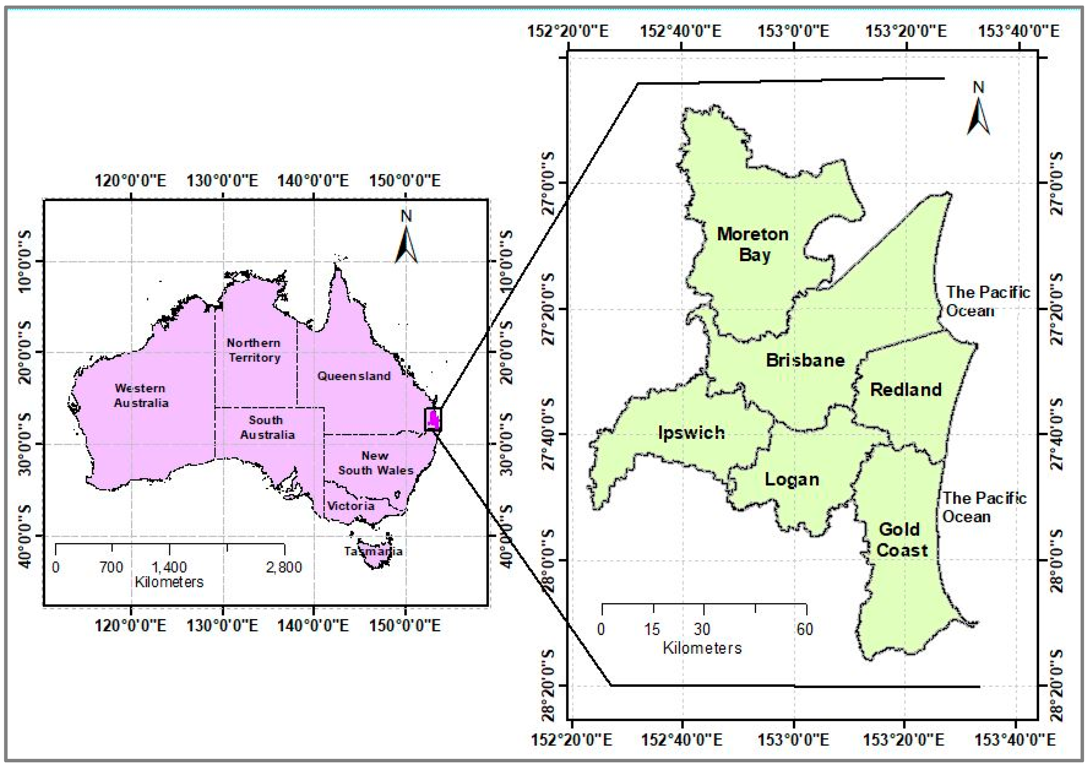
The local government area (LGA) of Brisbane and its surrounding LGAs covering an area of about 8556 km² are chosen as the case study area in order to determine the impacts of anthropogenic activities on climate change. The study area comprises LGAs of Brisbane, Gold Coast, Moreton Bay, Redland, Logan, and Ipswich (Figure 1). The reasons that motivate us to select this region as the testbed are as follows: (a) the selected LGAs are located in the state of Queensland, where the state was subjected to nearly 60% of the nation’s land clearing over the last four decades (Steffen & Dean, 2018); (b) Queensland has been generating about 80% of the nation’s land use emissions (Steffen & Dean, 2018), which has substantial impacts on local climate change; (c) the selected LGAs are the most urbanized part of the state [37]; (d) Brisbane ranks as the most sprawling city in Australia [38,39]; (e) while Brisbane’s urban areas only accommodate 6% of the national population [40], its low-density urban expansion to nearby peri-urban areas places a great risk on the ecosystem services [41], and; (f) Brisbane is claimed to be one of the most sustainable and smart cities in Australia [42,43,44].

2.2. Data

Four Landsat images corrected at level-one terrain (L1T) level were used to detect the climate change impacts triggered by anthropogenic activities for a period of 30 years with 10-year intervals [45] (

Table 1. Characteristics of Landsat data.

Date	Path/row	Sensor	Satellite	Resolution
16 Sep 1989	89/79	TM	Landsat 5	30m
19 Aug 1999	89/79	ETM+	Landsat 7	30m
23 Sep 2009	89/79	TM	Landsat 5	30m
3 Sep 2019	89/79	OLI	Landsat 8	30m

).

The estimated resident population (ERP) data of the Australian Bureau of Statistics (ABS) were used to investigate the socioeconomic aspects of anthropogenic activities. In the case of calculating GHG emissions due to anthropogenic activities, this study used the national GHG inventory database of the Australian government—AGEIS [46]. In order to reveal the changes in precipitation and temperature over time, data were taken from the Australian Bureau of Meteorology (BoM).

2.3. Methods

2.3.1. Landsat Image Classification and Performing Accuracy Assessment

Multispectral Landsat images processed at L1T level were classified into four land use and land cover (LULC) categories, namely, bare soil (i.e., exposed soil, vacant lands, sand), built-up (i.e., transportation networks, industrial, residential, institutional settlements, commercial), vegetation (i.e., playground, parks, greeneries, trees), and water body (i.e., lakes, reservoirs, retention ponds, coastal water, rivers) [47]. In order to derive the abovementioned LULC classes, the maximum likelihood supervised classification (MLSC) technique was applied. Nearmap data with 5.8–7.5 cm spatial resolution, Google Earth imageries, and field survey data were utilized collectively to develop training samples required to perform the MLSC technique in the ENVI image analysis software.

For carrying out accuracy assessments of the classified images, 350 stratified random sampling points were generated in the ArcGIS software. Afterwards, ground-truthing of the classified images were performed using field surveys, Nearmap data, and Google Earth images. Then, error matrices were produced to check the accuracy of each classified image. The image classification process was repeated by using different training samples until the threshold accuracy of 85% for each classified image was achieved [48]. The error matrices of each classified image are presented in

Table 2. The error matrix for the classified image of 1989.

LULC Category	Ground Truth Points	LULC Data Points	Number Correct	Producer’s Accuracy	User’s Accuracy
Bare soil (total count)	77	72	65	90.28%	84.42%
Built-up (total count)	50	51	45	88.24%	90.00%
Vegetation (total count)	168	174	160	91.95%	95.24%
Water body (total count)	55	53	49	92.45%	89.09%
Grand total points count	350	350	319
Overall accuracy	91.14%
Kappa coefficient	0.87

,

Table 3. The error matrix for the classified image of 1999.

LULC Category	Ground Truth Points	LULC Data Points	Number Correct	Producer’s Accuracy	User’s Accuracy
Bare soil (total count)	54	53	47	88.68%	87.04%
Built-up (total count)	69	69	61	88.41%	88.41%
Vegetation (total count)	170	173	158	91.33%	92.94%
Water body (total count)	57	55	49	89.09%	85.96%
Grand total points count	350	350	315
Overall accuracy	90%
Kappa coefficient	0.85

,

Table 4. The error matrix for the classified image of 2009.

LULC Category	Ground Truth Points	LULC Data Points	Number Correct	Producer’s Accuracy	User’s Accuracy
Bare soil (total count)	61	58	52	89.66%	85.25%
Built-up (total count)	84	89	78	87.64%	92.86%
Vegetation (total count)	148	148	139	93.92%	93.92%
Water body (total count)	57	55	52	94.55%	91.23%
Grand total points count	350	350	321
Overall accuracy	91.71%
Kappa coefficient	0.88

and

Table 5. The error matrix for the classified image of 2019.

LULC Category	Ground Truth Points	LULC Data Points	Number Correct	Producer’s Accuracy	User’s Accuracy
Bare soil (total count)	75	72	64	88.89%	85.33%
Built-up (total count)	79	81	71	87.65%	89.87%
Vegetation (total count)	126	129	118	91.47%	93.65%
Water body (total count)	70	68	63	92.65%	90.00%
Grand total points count	350	350	316
Overall accuracy	90.29%
Kappa coefficient	0.87

.

2.3.2. Estimating Changes Due to Anthropogenic Activities

Identifying Major LULC Changes

This study investigated urbanization-led major LULC changes which exert significant influence on climate change. In the case of determining the major LULC changes, the study considered the LULC transitions as major which were more than 50 km² between 1989 and 2019. Such changes comprise four major LULC transitions in particular—i.e., vegetation to bare soil (VEG_BS), vegetation to built-up (VEG_BU), bare soil to built-up (BS_BU), and bare soil to vegetation (BS_VEG). By using TerrSet, this study quantifies these four major transitions.

Calculating Ecosystem Service Value Losses

In order to derive the impact of urban expansions on ecosystem services, the study quantified the losses in ESV over time. In this connection, this study used Sandhu et al.’s [49] ESV estimate of the New Zealand context in order to calculate the losses in ESV for the Australian context.

Besides, this study used the consumer price index (CPI) value to adjust Sandhu et al.’s [49] estimation of ESV. The following equation was used for this adjustment:

ESV₂₀₁₉ = ESV₂₀₁₂ × (CPI₂₀₁₉/CPI₂₀₁₂)

(1)

where ESV₂₀₁₉ = adjusted ESV of the year 2019; ESV₂₀₁₂ = Sandhu et al.’s [49] estimation of ESV; CPI₂₀₁₉ = CPI value of the year 2019; CPI₂₀₁₂ = CPI value of the year 2012.

Thus, ESV₂₀₁₉ = 3224 × (258.68/229.59) = USD 3632.40 [50]. This adjusted ESV₂₀₁₉ was used to calculate the net losses in ESV that occurred in the decades of 1989–1999, 1999–2009, and 2009–2019.

The net deforestation that took place for each 10-year intervals—i.e., 1989–1999, 1999–2009, 2009–2019—was calculated by using the following equation:

Net deforestation = (Vegetation to bare soil + Vegetation to built-up) – Bare soil to vegetation

(2)

Calculating Greenhouse Gas Emissions

To quantify urbanization-led GHG emissions, this study utilized ‘Australian GHG information system’ (AGEIS) data to derive GHG emissions per capita, which was later used to derive GHG emissions/ha due to urbanization-led major LULC changes.

While calculating GHG emissions, the study hypothesized the following:

▪

The conversion of vegetation to built-up areas undergoes two consecutive steps: First, the conversion of vegetation to bare soil (i.e., deforestation); second, the conversion of bare soil to built-up areas.

▪

Total GHG emissions from each major LULC conversion comprise two parts: (a) conversion-related emissions; (b) GHG emissions from the end LULC category. For example, in the case of the conversion from vegetation to built-up areas, GHG is emitted from two sources: (i) the emitted GHG due to the conversion of vegetation to built-up areas, and; (ii) the emitted GHG from the end LULC category—i.e., existing built-up areas.

▪

The specific time frame within which an LULC transition occurred and the time frame since subsequent GHG is emitted from the end LULC category are unknown. Hence, in estimating the rate of GHG emissions/ha, conversion-related GHG emissions and subsequent GHG emissions from the end LULC category were calculated altogether.

▪

The GHG emissions related to the conversion of bare soil to vegetation (that can be termed as ‘revegetation’) were ignored, as such a transition-related emission was insignificant. For example, in 2016, Queensland’s revegetation-related GHG emission was only 0.009 tonnes/capita [46]. Hence, only the end LULC GHG sink from the conversion of bare soil to vegetation—i.e., “space of carbon sink”—is considered, which is 5 tonnes/hectare/annum [51].

▪

Deforestation (that is due to the conversion of vegetation to bare soil (VEG_BS)) and urbanization-led conversions—i.e., bare soil to built-up areas (BS_BU) and vegetation to built-up areas (VEG_BU)—were considered as sources of GHG emissions. On the other hand, the conversion of bare soil to vegetation was considered as a space of carbon sink.

▪

Bare soil was considered as no land use activity and, hence, no emission from bare soil was calculated.

The GHG emissions data were gathered from AGEIS [46]. Queensland’s estimated resident population (ERP) of each corresponding year was used to derive per capita GHG emissions for each selected LULC transition. The average of per capita GHG emissions of the Queensland state between each 10-year period (e.g., between 1999 and 2009) was later on used to derive GHG emissions originated from the urbanization-led LULC changes in the context of the study area.

In order to calculate GHG emissions stemmed from the conversion of vegetation to built-up areas, emissions from deforestation, construction emissions, and household emissions (such as from energy usage, and solid waste disposal), direct non-agricultural (NA) residential emissions, and indirect emission (i.e., emissions from purchased electricity) were considered. While calculating GHG emissions due to the conversion of bare soil to built-up areas, all above-mentioned sources of GHG emissions except for deforestation were used. In order to calculate GHG emissions due to the conversion of vegetation to bare soil, only the emissions attributable to deforestation were considered.

Finally, the aggerate GHG emissions figure was calculated by estimating the emissions released from the LULC, which did not change over time (i.e., ‘built-up areas’ and ‘vegetation’ showing persistence) and the emissions from major LULC changes over the investigated 30-year period.

Checking the Reliability of GHG Estimation Approaches

In order to crosscheck the reliability of our GHG estimation approaches, we specifically calculated GHG emissions for the LGA of Brisbane. The Brisbane LGA was selected for this examination because such relevant data for comparison were available for this LGA from secondary resources.

Calculating the Variations in GHG Emissions between Unquestionably Urban, Peri-Urban, and Rural Areas

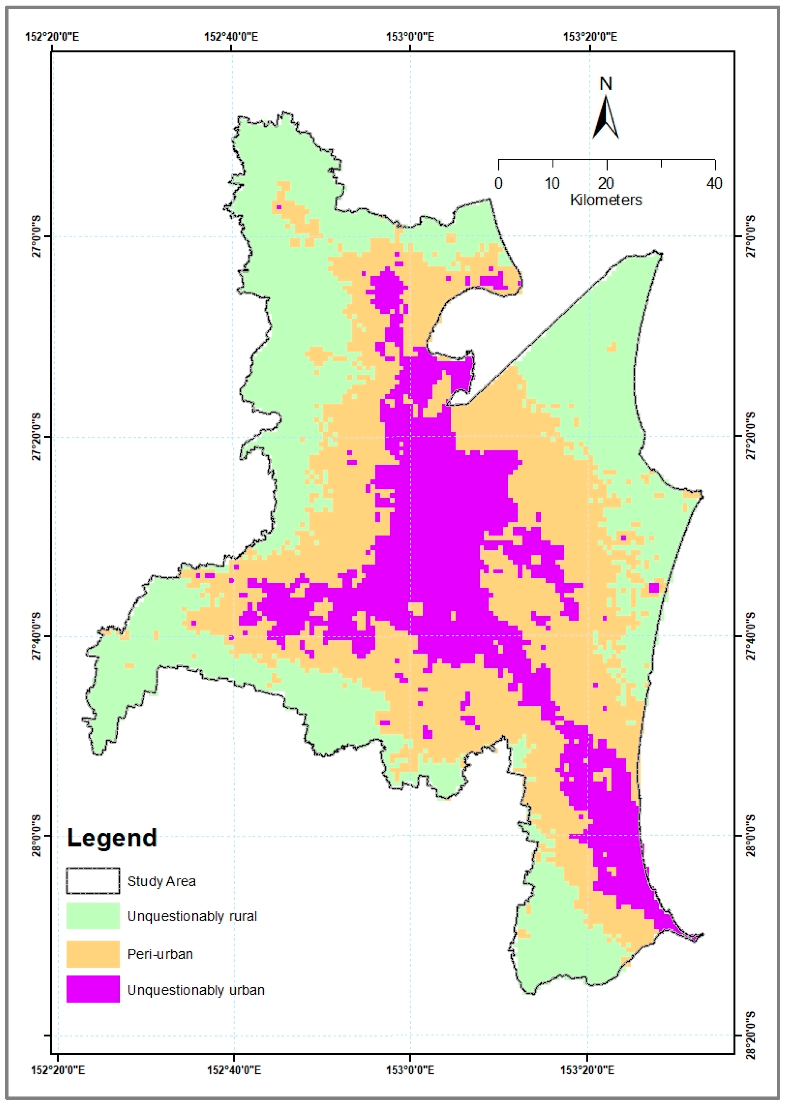
In order to determine the spatial distribution of GHG emissions within different urban growth land use areas, this paper adopts Mortoja et al.’s [23] study approach to demarcate unquestionably urban, peri-urban, and rural areas. They applied fuzzy logic on night-time light (NTL) data to demarcate these urban growth areas. This study applied their methodological approach to demarcate different urban growth areas for the year 2019 by using NTL data of 2019 (Figure 2). Later, this study estimated GHG emissions within the demarcated urban growth areas between 1989 and 2019. While estimating per capita GHG emissions for each LULC transition between 1989 and 2019, the study took the average value of per capita GHG emissions of the three decades.

2.3.3. Changes in Atmospheric Temperature and Precipitation

The study at hand did not directly measure the fraction of climate change attributable to major LULC changes. Nevertheless, we looked at the general trend of temperature and precipitation pattern between 2000 and 2020, which appear to help in anticipating the anthropogenic climate change impacts indirectly.

2.3.4. Shifts in State Polices and Corresponding Deforestation

In order to illustrate the policy impacts influencing deforestation, this study looked at how the state policies governed deforestation, and how these incurring deforestations resulted in increased GHG emissions over time.

3. Results

3.1. Changes in Land Use and Land Cover

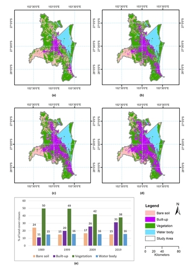
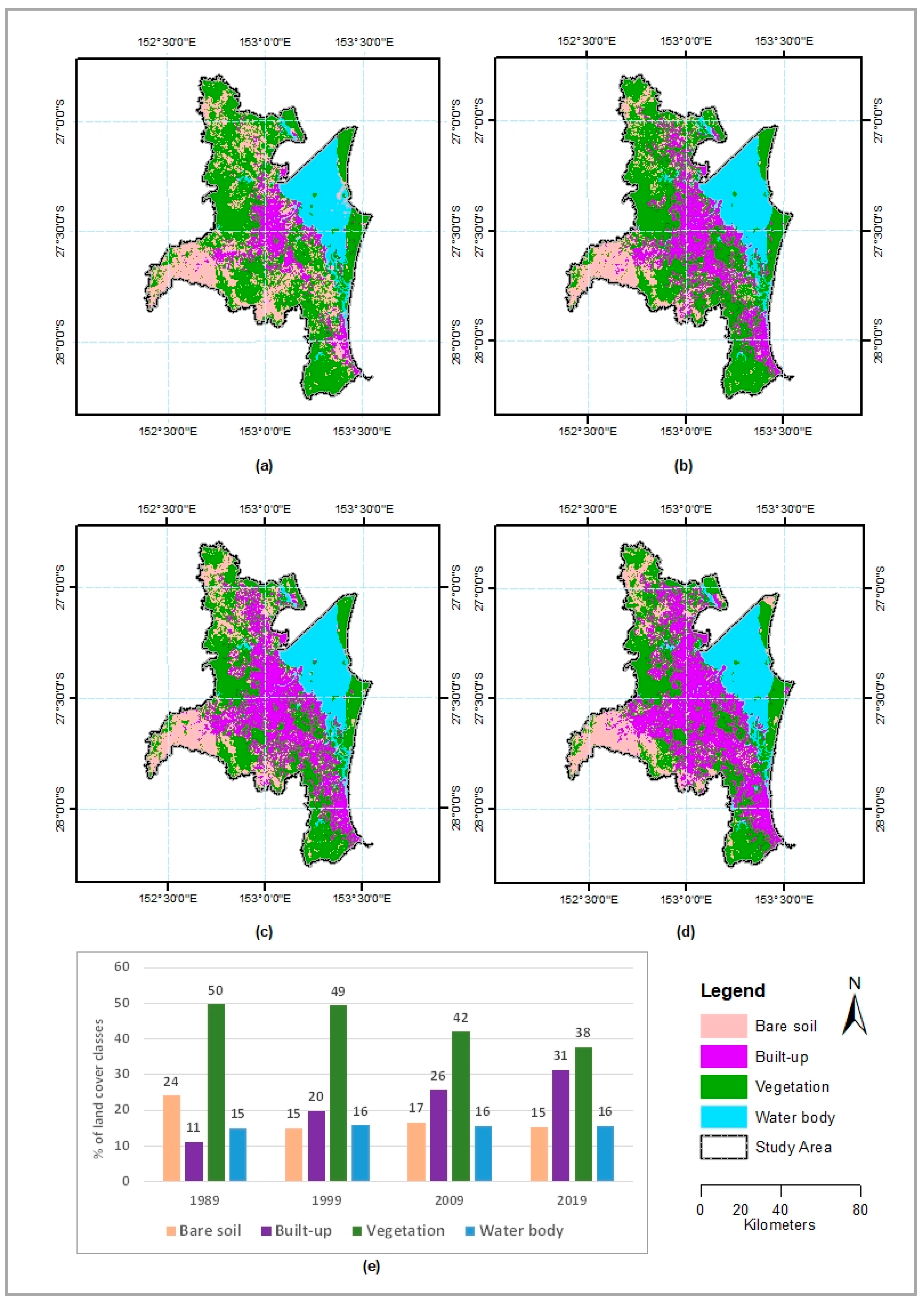
The classified LULC images are presented in Figure 3, while the percentage of LGA share of total LULC changes for 1989, 1999, 2009 and 2019 is depicted in Figure 4. Between 1989 and 2019, built-up areas increased by nearly 1711 km² (20% of the study area), bare soil declined by approximately 513 km² (6% of the area), and vegetation decreased by about 1027km² (12%) (Figure 3e). In 1999, built-up areas experienced the highest growth of 9% from the base year estimate of 1989, whereas from 1999 to 2019, built-up areas collectively gained a growth of 11%. Interestingly, between 1989 and 1999, bare soil declined by 9%, and such a decline in vegetation within this time frame was only 2%—indicating the period undergoing brownfield development.

Between 1999 and 2009, built-up areas increased by 6% and vegetation declined by 7% with little changes in bare soil (i.e., only 2%), implying that this decade had undergone greenfield development. Between 2009 and 2019, vegetation and bare soil declined by 4% and 2%, respectively, while built-up areas increased by 5%, indicating that this period had undergone both brownfield and greenfield development.

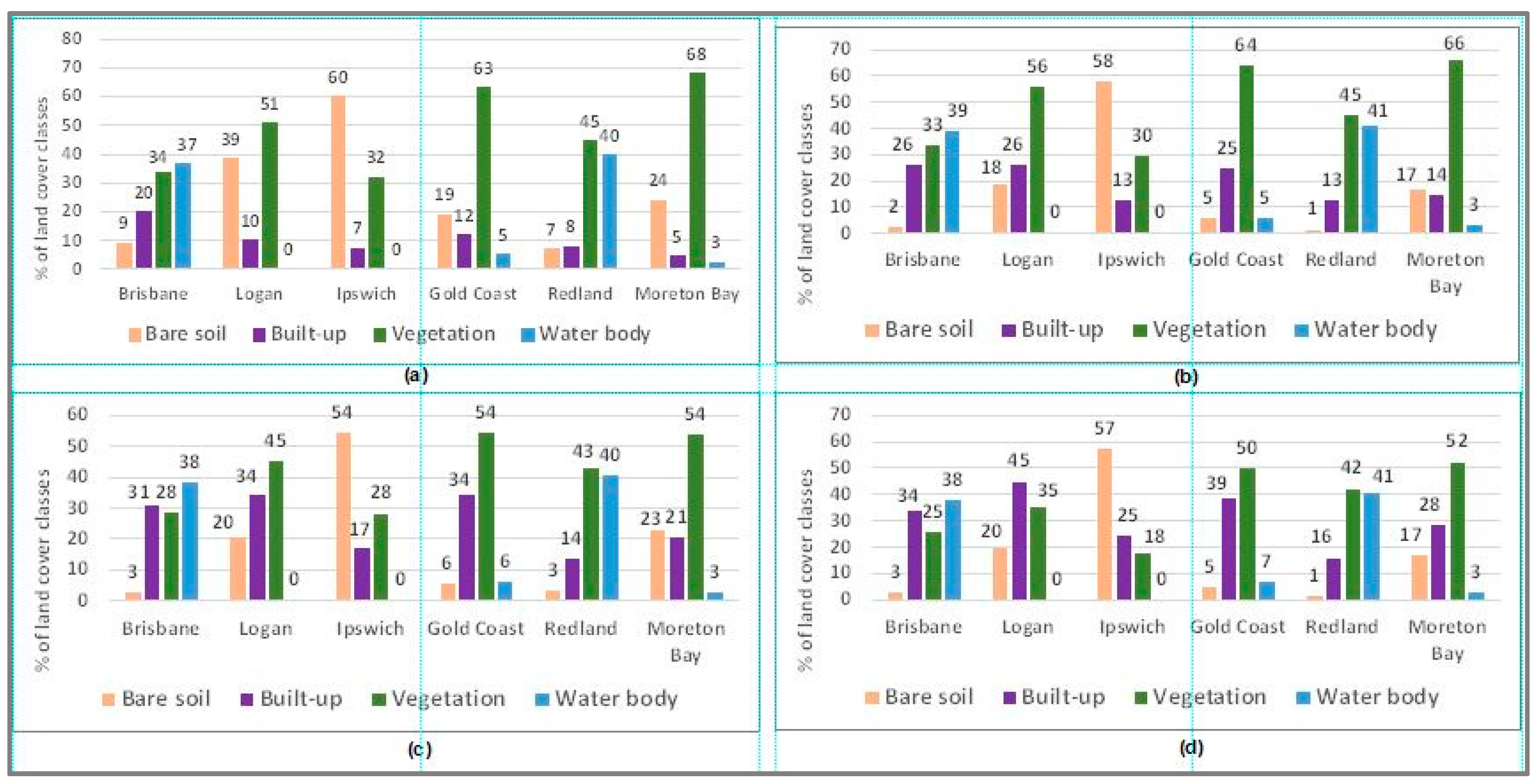
In terms of built-up areas growth within LGAs, Logan experienced the highest growth of 35% followed by Gold Coast (27%), and Moreton Bay (23%) between 1989 and 2019 (Figure 4). Within this 30-year period, Logan and Moreton Bay both also encountered the highest loss in vegetation (16%) followed by Ipswich (14%) and Gold Coast (13%). Again, in terms of bare soil, Logan experienced the most by 19%. Subsequently, throughout the 30-year period, Logan, Gold Coast and Moreton Bay experienced higher growth than Brisbane.

Brisbane comprises the highest amount of water body areas and its growth to the East is constrained by the Pacific Ocean. Consequently, Brisbane’s growth trickles down towards Moreton Bay at North, Logan at South, and Ipswich in the West. Nevertheless, 1% net increase in Brisbane’s water body between 1989 and 2019 does not imply sea-level-rise. Instead, such an increase might be attributed due to the underlying error in the image classification process.

Besides, Ipswich covers the highest amount of bare soil—which only declined by 3% over time. In contrast, vegetation in Ipswich declined by 14%, meaning bare soil in Ipswich is not suitable for development due to the presence of some natural constraints. In reality, a large chunk of bare soil in Ipswich yet remains undeveloped, as these are declared as grazing area and some portions are conserved as ecologically sensitive areas. Thus, overgrazing might lead to more bare soil formation in Ipswich, which warrants further research.

3.2. Changes in Land Use and Land Cover and Ecosystem Service Values

The 1999–2009 period demonstrated the highest deforestation (i.e., 71,543 ha) and ESV losses (i.e., 2.6 billion)—which is around 7.5 times higher than that of the 1989–1999 period (

Table 6. LULC transitions and ecosystem service value changes over the 30-year period.

Major Land Cover Changes	1989–1999	1999–2009	2009–2019
Bare soil to built-up (BS_BU) (ha)	53,681	16,697	32,481
Bare soil to vegetation (BS_VEG) (ha)	44,877	14,787	11,242
Vegetation to bare soil (VEG_BS) (ha)	24,184	32,047	24,318
Vegetation to built-up (VEG_BU) (ha)	30,234	54,283	30,776
Net deforestation (ha)	9541	71,543	43,852
Net ESV losses (USD billion)	0.35	2.60	1.59
Percentage of ESV losses	7.7	57.27	35.02

). More than 57% of ESV were lost in the 1999–2009 decade. From 1999 to 2009, the transition from vegetation to built-up area was 54,283 ha, which is around 1.8 times higher than those that occurred in the 1989–1999 and 2009–2019 periods. On the contrary, the conversion from bare soil to vegetation in the 1989–1999 decade was 44,877 ha, which is around three and four times higher than those of the 1999–2009 and 2009–2019 decades, respectively. The 1989–1999 period is also the lowest in terms of converting vegetation to bare soil, which led to the smallest value in deforestation (i.e., 9541 ha) and subsequent losses in ESV (0.35 billion) in the 1989–1999 period.

3.3. Changes in Land Use and Land Cover and Greenhouse Gas Emissions

Queensland’s per capita GHG emissions for each selected LULC transition over time are presented in

Table 7. Estimating urbanization-led built-up greenhouse gas (GHG) emissions of Queensland, derived from AGEIS [46] and Queensland government [52]

Year	Direct GHG Emissions (1000 Tonnes)					Indirect GHG Emission (1000 tonnes)	Total GHG Emission (1000 tonnes)	Estimated Resident Population (ERP)	GHG (per Capita) for ‘Bare Soil to Built-Up’	GHG (per Capita) for ‘Vegetation to Built-Up’	GHG (per Capita) for ‘Vegetation to Bare Soil’
	Energy	Solid Waste Disposal	Deforestation	Construction	Non-Agricultural Residential
1990	48,542	3324	31,123	1865	7449	33.38	97,770	2,928,713	22.76	33.38	10.63
1999	71,218	3010	51,016	1814	8560	40.98	143,312	3,497,147	26.39	40.98	14.59
2009	98,636	3165	29,740	1716	11,563	34.81	154,431	4,436,882	28.10	34.81	6.70
2016	112,689	2214	16,224	2165	13,502	31.90	155,795	4,883,821	28.58	31.90	3.32

, while the estimated GHG emissions/ha/annum for these selected LULC transitions are highlighted in

Table 8. Estimating GHG emissions for the changes of ‘bare soil to built-up (BS_BU)’, ‘vegetation to built-up (VEG_BU)’, and ‘vegetation to bare soil (VEG_BS) for the study area.

Indicator	1989–1999	1999–2009	2009–2019
Average GHG /per capita (tonnes/per capita) (for BS_BU)	24.57	27.25	28.34
Average GHG /per capita (tonnes/per capita) (for VEG_BU)	37.18	37.9	33.36
Average GHG /per capita (tonnes/per capita) (for VEG_BS)	12.61	10.65	5.01
Changes in population	324,100	512,054	541,354
Bare soil to built-up (BS_BU) (ha)	53,681	16,697	32,481
Vegetation to built-up (VEG_BU) (ha)	30,234	54,283	30,776
Vegetation to bare soil (VEG_BS) (ha)	24,184	32,047	24,318
Bare soil to vegetation (BS_VEG) (ha)	44,877	14,787	11,242
Sum of major LU transitions	152,976	117,814	98,817
Ratio of BS_BU = BS_BU/Sum of major LULC transitions	0.35	0.14	0.33
Ratio of VEG_BU = VEG_BU/Sum of major LULC transitions	0.20	0.46	0.31
Ratio of VEG_BS = VEG_BS/Sum of major LULC transitions	0.16	0.27	0.25
Increased GHG for BS_BU= (changes in population × average GHG/capita for BS_BU X ratio of BS_BU)	2,794,805	1,977,337	5,043,018
Increased GHG for VEG_BU = (changes in population × average GHG/capita for VEG_BU X ratio of VEG_BU)	2,381,556	8,941,737	5,624,552
Increased GHG for VEG_BS = (changes in population × average GHG/capita for VEG_BS X ratio of VEG_BS)	645,962	1,482,759	667,777
GHG emission for BS_BU/ha/annum	5.21	11.84	15.53
GHG emission for VEG_BU/ha/annum	7.88	16.47	18.28
GHG emission for VEG_BS/ha/annum	2.67	4.63	2.75

. Our analysis reveals that GHG emissions/ha/annum related to the conversion of built-up areas from bare soil and vegetation increased over time, with a more than two-fold increase in the 1999–2009 decade than those of the 1989–1999 decade. Nevertheless, deforestation-related GHG emissions/ha/annum was highest (i.e., 4.63 tonnes/ha/annum) in the 1999–2009 decade, which is around 1.7 times higher than its former and later decades.

In terms of per hectare aggregate GHG emissions, the analysis shows that such an emission was lowest (i.e., 2.34 tonnes/ha/annum) in the 1989–1999 decade but was quadrupled in the 1999–2009 decade (

Table 9. Calculating aggregate GHG emissions in the study area.

Persistent	LULC Category/Transition	Area (ha)			GHG Emissions (tonnes)
		1989–1999	1999–2009	2009–2019	1989–1999	1999–2009	2009–2019
	Built-up (≈ BS_BU) (+)	84,135	146,933	201,475	4,383,429	17,396,838	31,289,063
	Vegetation (carbon sink) (−)	367,552	333,902	300,892	18,377,616	16,695,117	15,044,608
	Sub-total (persistent)	451,687	480,835	502,367	(−)13,994,187	701,721	16,244,455
Major Transitions	Bare soil to built-up (ha) (+)	53,681	16,697	32,481	2,796,785	1,976,874	5,044,278
	Bare soil to vegetation (ha) (i.e., carbon sink) (-)	44,877	14,787	11,242	2,243,849	739,331	562,099
	Vegetation to bare soil (ha) (+)	24,184	32,047	24,318	645,720	1,483,770	668,741
	Vegetation to built-up (ha) (+)	30,233	54,283	30,776	2,382,398	8,940,384	5,625,844
	Sub-total (major LULC transitions)	152,976	117,813	98,817	3,581,054	11,661,697	10,776,763
Grand total		604,663	598,648	601,184	(-)10,413,132	12,363,417	27,021,218
Per Unit GHG calculation	GHG/ha/annum (for major LULC transitions)				2.34	9.90	10.91
	Aggregate GHG/ha/annum				(-)1.72	2.07	4.49
	Total carbon sink	412,429	348,689	312,134	20,621,465	17,434,448	15,606,707
	Carbon source to sink ratio (in terms of area)	0.47	0.72	0.93
	Carbon source to sink ratio (in terms of aggregate GHG emissions)				0.50	1.71	2.73

). Nonetheless, albeit per hectare aggregate GHG emissions increased over time, such an increase did not demonstrate significant variation between the periods of 1999–2009 and 2009–2019.

As for the case of aggregate GHG emissions/ha/annum, due to the prevalence of vegetation coverage, aggregate GHG emissions/ha/annum were found negative (i.e., –1.72 tonnes/ha/annum) in the 1989–1999 decade, indicating that aggregate GHG emissions were offset by the amount of carbon sink. Nonetheless, aggregate GHG emissions/ha/annum were highest (i.e., 4.49 tonnes/ha/annum) in the period of 2009–2019, which is more than two times higher than to its former 10-year period of 1999–2009.

The carbon source to sink ratio (in terms of area coverage) increased over time, but always remained below 1.0, indicating that the coverage of vegetation was always higher than those of carbon sources throughout the decades. Contrastingly, the carbon source to sink ratio, in terms of aggregate GHG emissions, was below 1.0 in the 1989–1999 decade, but increased to 1.71 and 2.73 by the periods of 1999–2009 and 2009–2019, respectively. Therefore, the period of 1989–1999 released the least aggregate GHG emissions/ha/annum.

3.4. Checking the Reliability of GHG Estimation Approaches

Our estimated GHG emissions figures, that originated from the persistent built-up area category and major LULC transitions for the LGA of Brisbane between 2009 and 2019, are calculated as 2.8 tonnes/annum (

Table 10. Calculating Brisbane’s GHG emissions that originated from the persistent built-up area category and major LULC transitions.

LULC Category/Transition	Area (in ha)	GHG Emissions (tonnes)
	2009–2019	2009–2019
Built-up (persistent ≈ BS_BU)	63,235	9,820,398
Bare soil to built-up	2571	399,298
Vegetation to bare soil	2440	67,105
Vegetation to built-up	5655	1,033,747
Total GHG emissions		11,320,549
Population increases from 2009 to 2019 [55]		410,000
GHG emissions/capita/annum		2.8

). On the other hand, Brisbane’s overall per capita of GHG emissions is indicated in the literature as 14 tonnes/annum [53]. As household emissions for the Australian context contribute to 12% of total emissions [54], Brisbane’s household emissions can be derived as (14) × (0.12) = 1.68 tonnes/capita/annum. Thus, our estimated GHG figures appear to be a bit higher than household emissions. Such an outcome is reasonable as we considered the construction- and deforestation-related emissions along with calculating household emissions.

3.5. Variations in GHG Emissions between Unquestionably Urban, Peri-Urban, and Rural Areas

In terms of urban growth land use classification which sources GHG emissions, peri-urban areas comprise the biggest chunk (i.e., 36.17%) followed by unquestionably rural areas and unquestionably urban areas account for 34.67% and 29.16%, respectively (

Table 11. Calculating GHG emissions within different urban growth land use areas between 1989 and 2019.

Persistent	LULC Category/Transition	Unquestionably Urban			Peri-Urban			Unquestionably Rural
		Area (ha)	%	GHG (tonnes)	Area (ha)	%	GHG (tonnes)	Area (ha)	%	GHG (in tonnes)
	Built-up	79,861	89.57	26,018,830	8385	9.40	2,731,773	911	1.02	296,957
	Vegetation	20,166	6.93	3,024,974	108,365	37.25	16,254,815	162,368	55.82	24,355,240
	Sub-total (persistence)	100,028	26.32	22,993,856	116,750	30.72	(−)13,523,042	163,280	42.96	(−)24,058,284
Major Transitions	Bare soil to Built-up	39,289	43.74	12,800,292	42,988	47.86	14,005,532	7536	8.39	2,455,337
	Bare soil to vegetation	2760	13.07	413,963	9432	44.67	1,414,814	8924	42.26	1,338,610
	Vegetation to bare soil	1597	4.18	160,498	11,497	30.11	1,155,469	25,085	65.70	2,521,031
	Vegetation to built-up	35,707	41.51	15,221,899	41,840	48.63	17,836,510	8482	9.86	3,615,920
	Sub-total (major transitions)	79,353	33.75	27,768,725	105,758	44.98	31,582,697	50,027	21.28	7,253,678
Grand total (GHG release -carbon sink)		179,380		50,762,581	222,508		18,059,655	213,307		(−)16,804,606
% of grand total		29.16		97.59	36.17		34.72	34.67		(−)32.31
Rate (tonnes/ha/annum)		9.43			2.71			(-)2.63

). Conversely, the persistence in built-up areas is mostly confined within unquestionably urban areas and peri-urban areas, account for 89.57% and 9.4%, respectively.

As for the case of major LULC transitions, the highest amount of transitions occurred in the category of peri-urban areas (i.e., 44.98%) followed by unquestionably urban areas (33.75%) and unquestionably rural areas (21.28%). Additionally, transitions to built-up areas—i.e., ‘bare soil to built-up’ and ‘vegetation to built-up’—are found to be the highest in peri-urban areas.

In terms of total GHG emissions between different urban growth areas, in unquestionably rural areas’ net GHG emissions are negative (i.e., –32.31%), indicating that the presence of vegetation coverage largely offsets the LULC-related GHG emissions. Besides, the results show that unquestionably urban areas emitted the highest emissions followed by peri-urban areas, and per hectare GHG emissions in unquestionably urban areas are about 3.5 times higher than those of peri-urban areas.

3.6. Changes in Atmospheric Temperature and Precipitation

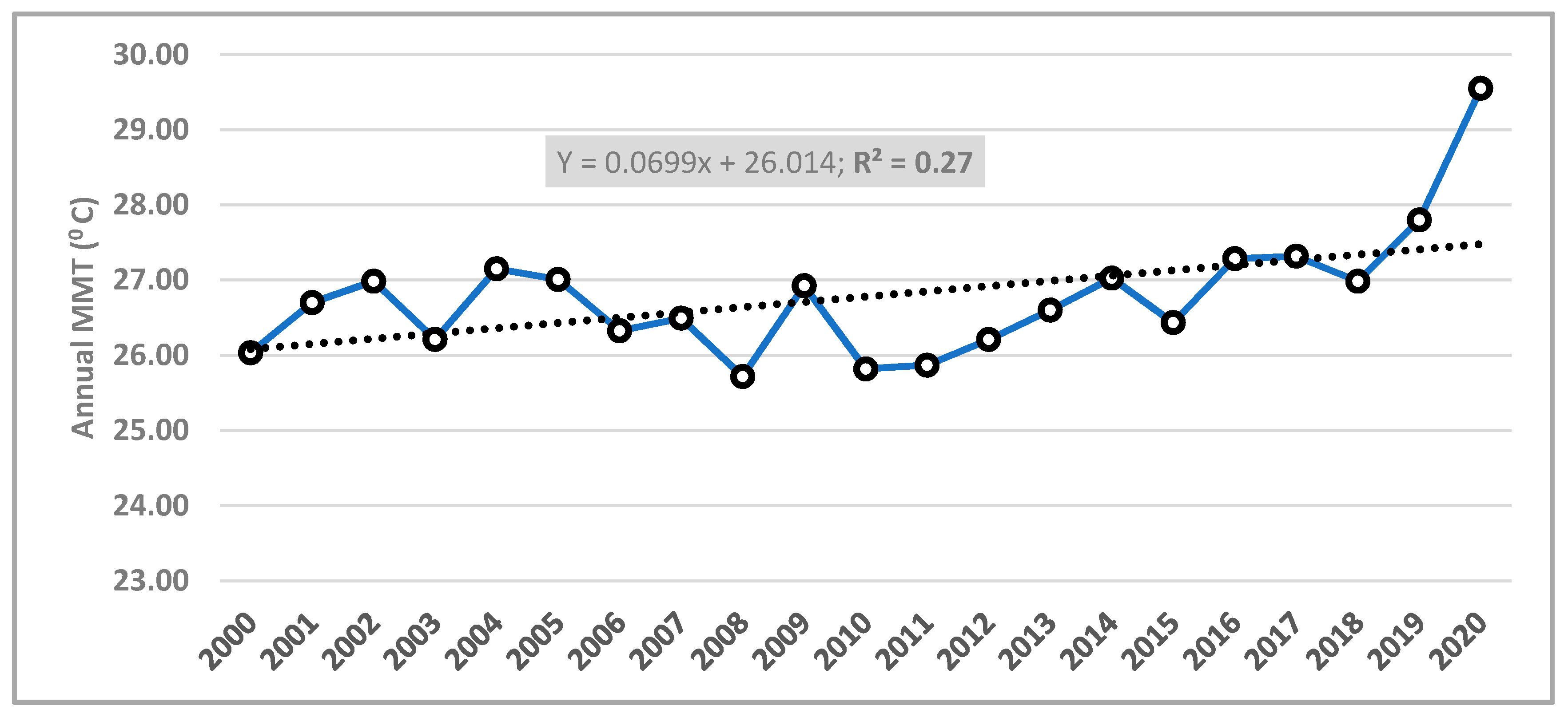
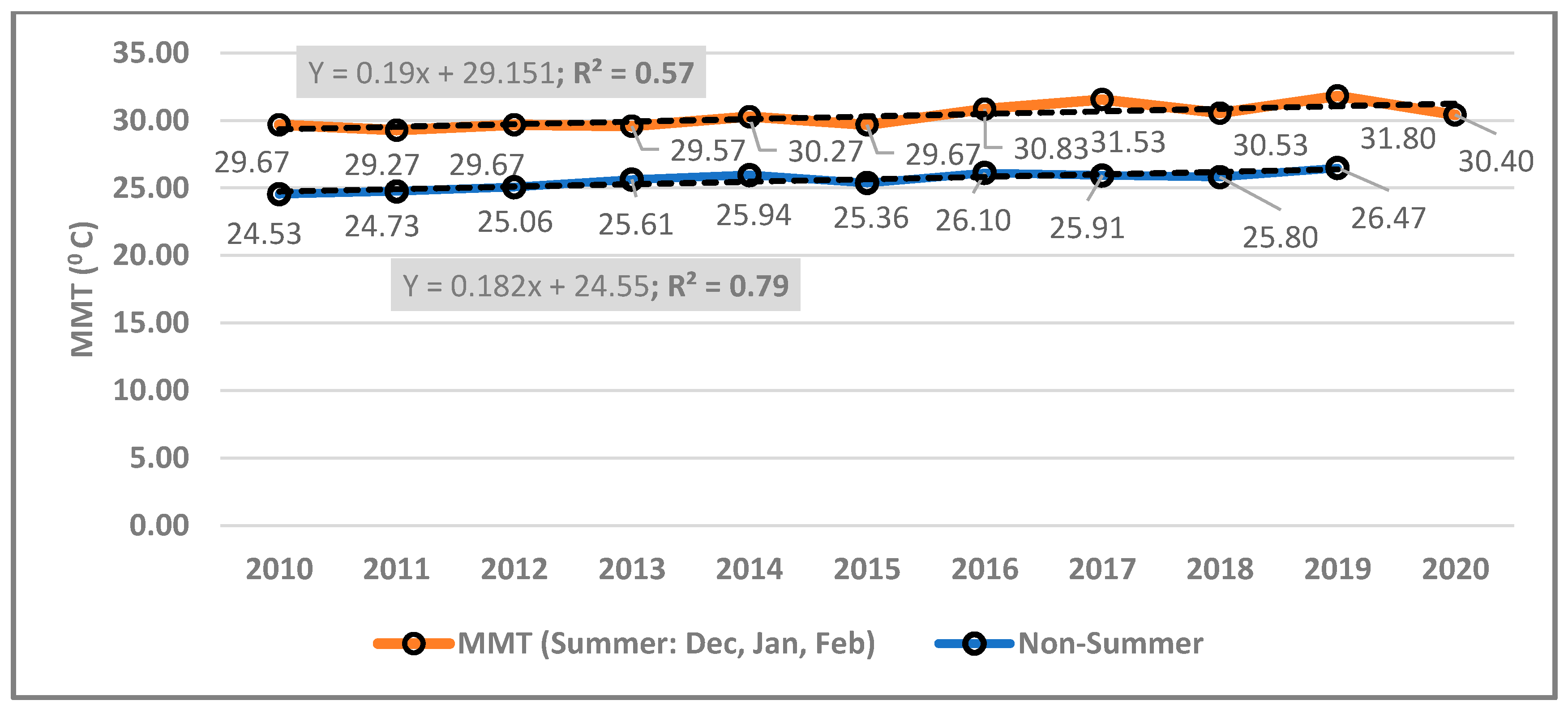
The increase in global temperature between the years 1900 and 2000 was approximately 0.7 °C, whereas the mean temperature increase value in Australia between the years 1910 and 2009 was more than 1 °C [56]. Australia is expected to experience 1 °C and 1.8 °C increases in atmospheric temperature by the year 2030 and 2050, respectively, from the base year estimate of 1990 [34]. Such an increasing trend of temperature has also been depicted from our study area, i.e., Brisbane and adjoining local government areas. While the study area experienced a slight increase in annual mean maximum temperature (MMT) between 2000 and 2020 (Figure 5), such temperature steadily increased during the last 10-year period (Figure 6). Although, the trend line of annual MMT shows a weak predictive level of acceptance (R² = 0.27), the substantial acceptance level of MMT for the non-summer season was found (R² = 0.79). Furthermore, the moderate predictive level of acceptance of MMT (R² = 0.57) was observed for the summer season.

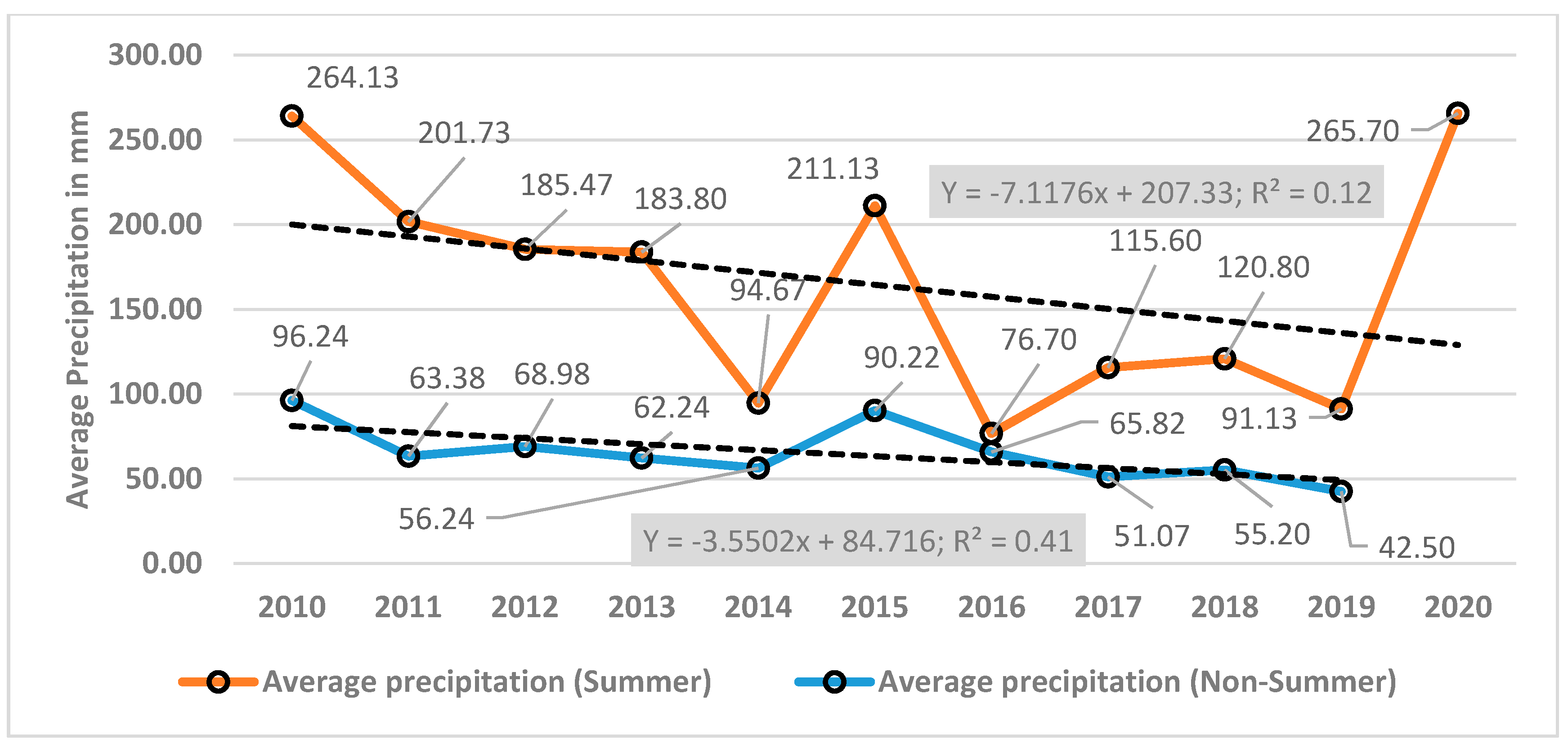
Moreover, Australia is also predicted to experience a decline in annual precipitation, and the rate of decrease in annual precipitation from the year 1970 to 2011 was 5mm/annum (Alamgir et al., 2014). In the context of our study area, this precipitation pattern showed a declining trend from 2010 to 2020 (Figure 7). While the trend of decline in average precipitation is weak (R² = 0.12) during the monsoon period, such a declining trend during the non-monsoon period is moderately significant (R² = 0.41).

Interestingly, in the Australian context, the monsoon period comes in the summer, which includes the months of December, January, and February due to the Southern Hemisphere positioning. Hence, these three months simultaneously represent both the summer and rainy seasons. Nonetheless, the increasing trend of MMT coupled with the decreasing trend of average precipitation appears to pose a detrimental effect on the growth of summer and non-summer agricultural products, e.g., fruits and vegetables.

3.7. Deforestation Scenarios Correspond to the Shifts in State Policies

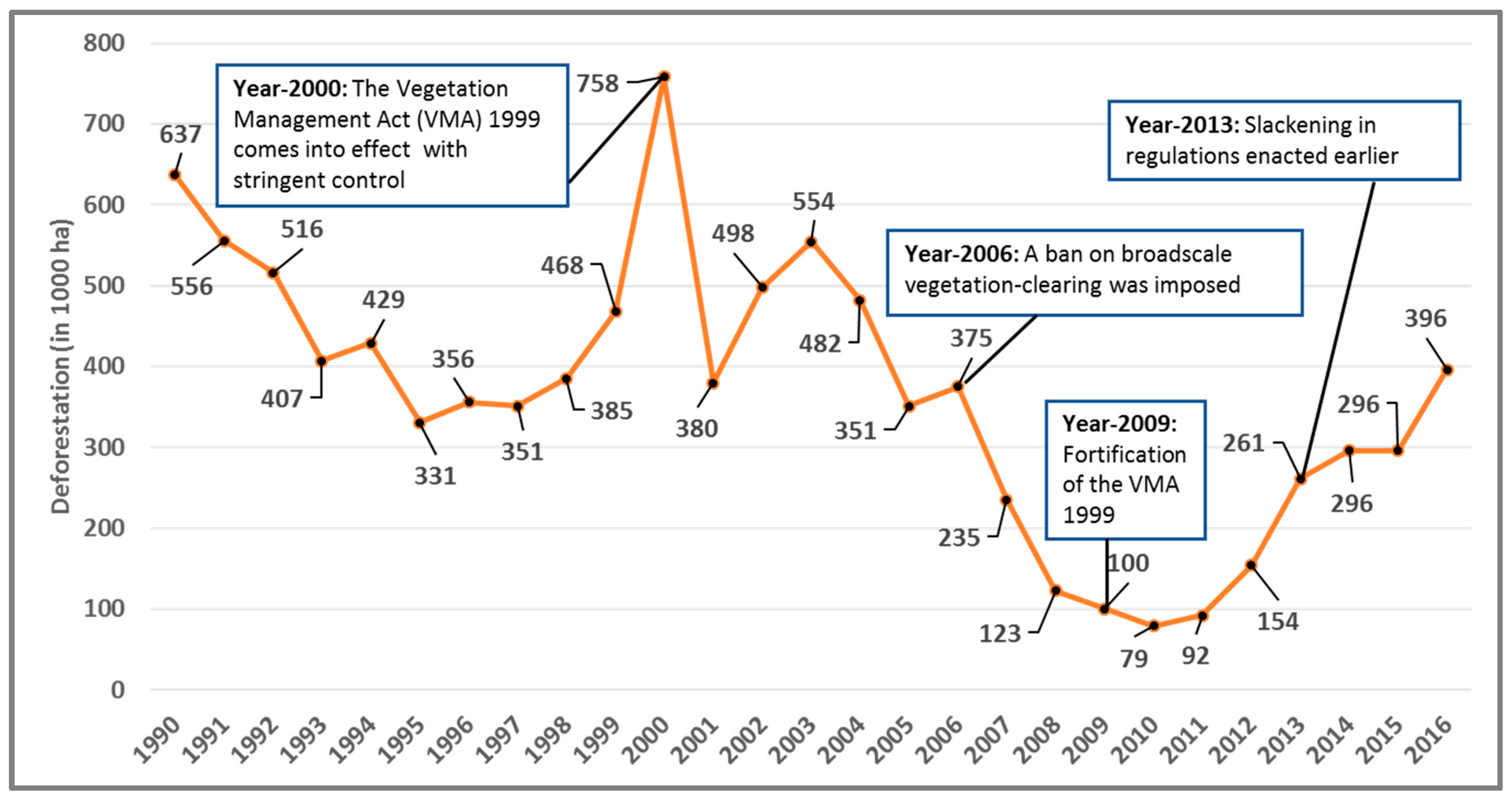
The state polices of Queensland concerning deforestation play a significant role in land clearing. (Figure 8). The amount of deforestation declined over time when stringent policy control on land clearing was imposed and later gained a sudden momentum when such strictly defined regulations were slackened.

For example, from 1990 to 1995, deforestation declined to 331,000 hectares from 637,000 hectares. Then, again in 2000, deforestation reached to its peak of 758,000 hectares. The Vegetation Management Act (VMA) 1999 curbed this amount to 375,000 hectares in 2006. Later in 2006, a ban on broad scale vegetation clearing was imposed, which resulted in a further decline to 100,000 hectares in 2009. In 2009, the Vegetation Management Act 1999 was further reinforced by giving additional emphasis to the protection of high-value regrowth vegetation. Such a reinforcement brought down the amount of vegetation clearing to a minimum of 79,000 hectares in 2010. Nonetheless, the Vegetation Management Amendment Act 2013, weakened the 2006 and 2009 regulations, leading to increased deforestation to 396,000 hectares in 2016.

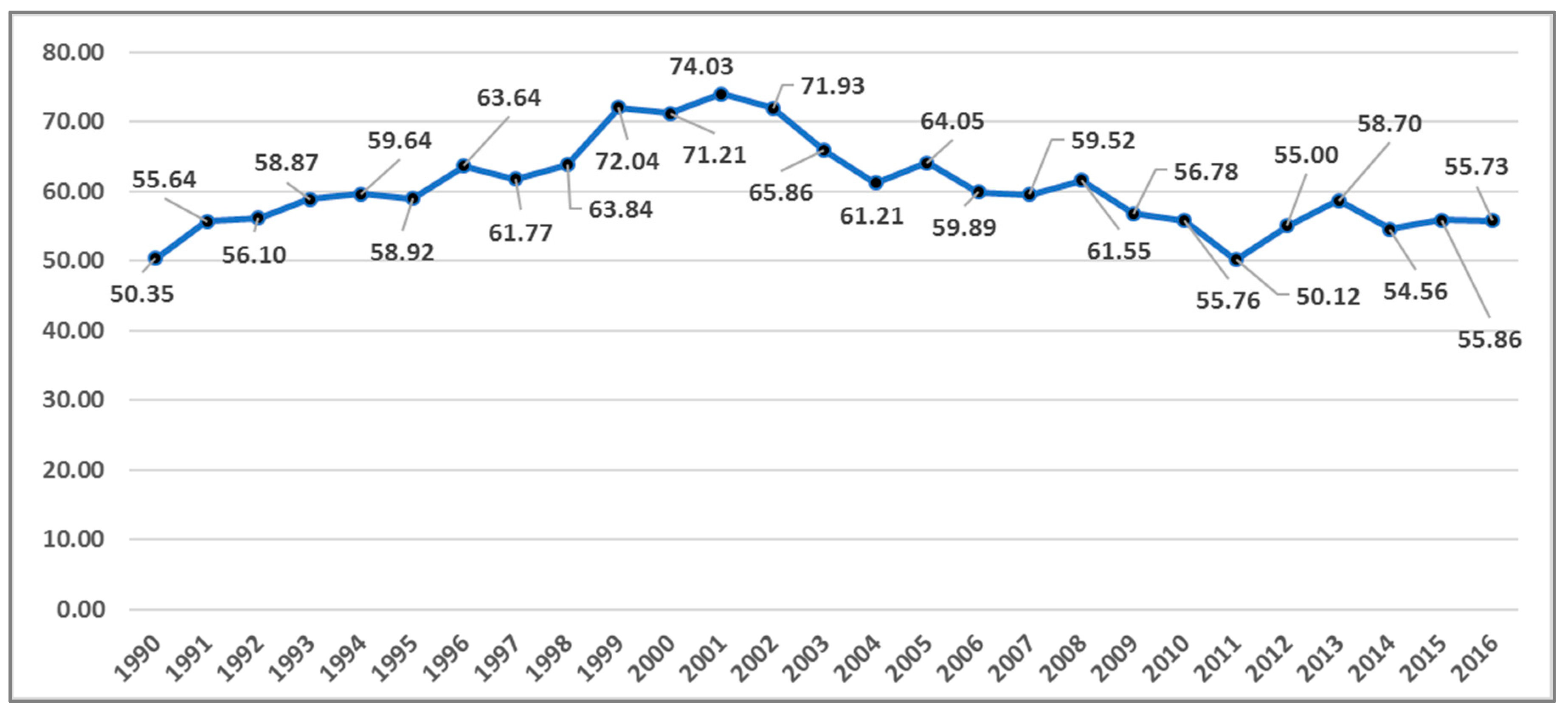
In terms of GHG emissions due to deforestation, Queensland shares the highest portion within Australia. For example, from 1990 to 2016, the percentage of Queensland’s deforestation-related share of national GHG emissions was always more than 50%, while such a share accounted for a minimum of 50.12% in 2011 (Figure 9). Yet, from 1990 to 1999, Queensland’s share increased to 72.04% from the base year estimate of 50.35% in 1990. In the periods of 1999–2009 and 2009–2016, such shares declined to 56.78% and 55.73%, respectively. In sum, from 1990 to 2001, such shares steadily increased and later started to decrease from 2002 to 2016.

4. Discussion

The study reported in this paper mainly focuses on peri-urbanization-related LULC changes and their impacts on ESV losses and GHG emissions. Nonetheless, ecosystem services, which lie within peri-urban farmlands, are the agroecosystem services. These agroecosystem services are undermined in the conventional ESV estimation process. The conventional ESV estimation approaches assign more weight on wetlands and assign nominal dollar values (i.e., USD 92/hectare/annum) to farmland ecosystem services inherent with peri-urban greenfield sites [14,58].

In general, more than 80% of the ecosystem service benefits cannot be monetized [59,60]. Thus, farmland ecosystem services are rich in values, but are highly discredited due to the inability to appropriately monetize these intangible service benefits. Furthermore, the global estimation approaches of ESV are backed-up by secondary data, which appears to be inappropriate in evaluating greenfield sites’ farmland ecosystem services at the regional/local context. Henceforth, Wu et al. [61] rightfully contend that peri-urbanization (which triggers the conversion of greenfield sites to bare soil and built-up areas) results in a significant decline in regional ESV. Thus, while conventional studies evaluate the loss of ESV due to the conversion of forested lands and wetlands to agricultural uses, our study analyses the loss of ESV due to the conversion of peri-urban farmlands to urban land uses.

The study at hand adopted Sandhu et al.’s [49] ESV estimation on agroecosystem services. They carried out regional estimation of ESV based on primary data and calculated ESV to farmland as USD 3224/hectare/annum—more than 35 times higher than that of Costanza et al.’s [14] global ESV estimation, which is commonly adopted in many studies [59].

Our ESV estimation approach relied on [49] ESV of the Canterbury Plains of New Zealand. Countries like New Zealand and Australia are both native vegetation dominated, and a large proportion of this vegetation is nonexistent elsewhere on the planet [62]. Besides, these two countries were separated from the rest of the globe for millions of years (ABS, 2010). Thus, because of their evolutionary and geographical detachments, both New Zealand and Australia have become biologically diverse from the rest of the globe [63]. Hence, ESV to farmlands for the contexts of New Zealand and Australia cannot be generalized with the global farmland estimation of ESV. Furthermore, New Zealand and Australia also inherit similar socioeconomic and cultural settings. Henceforth, ESV to farmlands for the Australian context appears to be equivalent to Sandhu et al.’s [49] estimation of farmlands’ ESV.

Our study area has undergone a significant brownfield development between 1989 and 1999, and then encountered a considerable greenfield development between 1999 and 2019. Such development trends reflected their corresponding consequences in ESV losses and GHG emissions, which collectively might induce the impact of anthropogenic climate change.

Nonetheless, the losses in ESV were conspicuous in the period of 1999–2009, and were lower during the 1989–1999 period. This is due to the extensive brownfield developments taking place between 1989 and 1999. Such a development pattern indicates a significant amount of vegetation coverage. In contrast, in the 1999–2009 period, the study area underwent greenfield development which was more than three times higher than the brownfield development that occurred between 1989 and 1999.

Such a development trend was also intensified by the mining boom in Australia in general. Between 2002 and 2012, Australia’s mining export had tripled, while spending contributed by the mining sector increased from 2% of gross domestic product (GDP) to 8% between this 10-year period [64].

Deforestation, which is a major catalyst of declining ESV, seems to be impacted by the Millennium Drought (2001–2009) event of Australia. However, anthropogenic influences on the drought event are not yet possible to determine, meaning that if there was an impact, such a proportion of anthropogenic influences on the drought event yet remains immeasurable. Consequently, the proportion of anthropogenic ESV losses attributable to the drought event also cannot be measured.

Nevertheless, ESV is determined based on four ecosystem services, namely, regulating services (e.g., climate regulation such as regulating the emissions of GHG), provisioning services (e.g., food production), supporting services (e.g., biodiversity habitat), and cultural services (e.g., amenity landscapes) [14]. Additionally, climate change-induced extreme heat events are strongly linked to human-led increased GHG emissions. The changes in LULC and ESV losses result in increased GHG emissions in the atmosphere.

Several studies quantified the impacts of human-led increased GHG emissions on extreme heat events. For example, researchers claimed that along with several past records of extreme heat events, the record-breaking heat events in Australia that occurred in summer of 1997–1998 and 2012–2013 were largely attributed to anthropogenic influences [65]. On that very point, the record-breaking Australian hot summers of 1997–1998 and 2012–2013 are estimated to have a minimum of seven-fold and five-fold increase, respectively, caused by anthropogenic climate change [66].

Furthermore, our analysis reveals that during the last decade (2010–2020), along with the declining precipitation trend, extreme heat events have also intensified and surpassed the previous record of extreme hot events. An increase in atmospheric temperature coupled with a decrease in annual precipitation leads to a drought event, which eventually impacts ecosystem services in the long run [67]. Besides, the climate impacts on ecosystem services are not uniform throughout Australia [35]—they varies across the regions both temporarily and spatially [68].

In the context of our study area, between 1989 and 1999, the gross emissions of GHG were negative, but 79,64,483 tonnes of GHG were collectively released from persistent built-up areas and due to the emissions from major LULC changes. In unquestionably urban areas, the percentage of vegetation coverage is insignificant, implying that extreme heat events are likely to be perceived more in unquestionably urban areas. On the other hand, the presence of the large stock of vegetation within unquestionably rural areas appears to lessen human-induced climate change impact within this zone, as the presence of vegetation is strongly linked to lowering the heat island effect [69,70,71,72]. However, the presence of vegetation can only lower the heat island effect by reducing the land surface temperature, that is, it cannot discernibly lessen the atmospheric temperature, which is substantially influenced by the impact of GHG emission-led anthropogenic climate change. Furthermore, the highest transition in LULC and corresponding GHG emissions occurred in peri-urban areas, meaning that peri-urbanization-related GHG emission plays a major role in overall GHG emissions.

Queensland’s deforestation scenarios and corresponding GHG emissions over time have been linked to policy control. Still, our study area experienced the highest ESV losses and GHG emissions between 1999 and 2009. Such losses in ESV and corresponding GHG emissions were apparently due to the mining boom that lasted from 2002 to 2012 and resulted in a massive urbanization drive. Hence, though Queensland’s land clearing regulations were tightened from 2001, investment spending via the mining boom outweighed land-clearing regulations in the context of our study area. However, this mining-led urbanization drive was later subdued due to the aftermath effect of the global financial crisis of 2007–2008. Consequently, we reported less LULC changes in the following period of 2009–2019 than those of the preceding 10-year period of 1999–2009.

In summary, the study discloses the following main findings: (a) the utilized remote sensing method is a useful technique in quantifying the impacts of climate change; (b) over the last 30-year period, Brisbane and its adjoining areas encountered a total loss of about USD 4.5 billion in ecosystem services due to direct and indirect anthropogenic climate change; (c) peri-urban areas encountered the biggest losses in ecosystem service values; (d) peri-urban areas experienced the highest greenhouse gas emission production levels, and; (e) ecosystem services should be backed up by robust urban management policies—this is critical for mitigating climate change.

5. Conclusions

As growth in urban areas in most of the metropolitan cities and regions around the globe are already saturated, peri-urban areas are now the potential pockets in accommodating further growth [73,74]. For that reason, peri-urbanization-driven ESV losses and GHG emissions should be taken into consideration.

The mix of urban and rural land uses accompanied by ambiguous land use patterns in peri-urban areas appears to quantify GHG emissions, and their corresponding impacts on GWP are challenging. Hence, quantifying peri-urbanization-driven GHG emissions remains unincorporated in the Intergovernmental Panel on Climate Change (IPCC)’s estimated climate change scenarios [75,76]. Still, globally occurring constant peri-urbanization to nearby greenfield sites and the corresponding changes in ESV and GHG emissions most likely will have an increasing climate change impact [77]. These peri-urban areas simultaneously serve both as a space of carbon sink and a carbon source. At inception, the vegetation dominating peri-urban areas serves as an ample source of ecosystem services, including the space of carbon sink. As urbanization goes by, carbon sink areas become minor over time and looming anthropogenic climate impacts become more visible.

Accordingly, identifying the locations experiencing constant losses in ESV and the locations shifting their role from a carbon reservoir to a carbon source within a peri-urban context is necessary to quantify the subsequent impacts of anthropogenic activities on climate change. Such impact identification will provide an evidence base to policymakers in formulating the most appropriate climate change mitigation strategies within peri-urban settings.

This study quantifies the spaces of carbon sources and carbon sinks over time. Simultaneously converting peri-urban areas hinder policymakers in identifying the GHG emissions emanating from anthropogenic sources, as differentiating carbon source areas is always difficult due to the dynamic nature of peri-urban areas [78,79]. Our study approach overcomes this limitation and helps estimate anthropogenic GHG emissions with increased precision. This way, our findings enable policymakers in deciding the level of vegetation coverage to be preserved in order to offset anthropogenic climate change impact due to increased GHG emissions.

The IPCC estimates mainly focuses on the climate change scenarios, while peri-urbanization-related GHG emission figures still remain uncovered. The unique contribution of this study is that it calculates peri-urbanization related GHG emissions and discloses that they are very high to the extent that they endanger the sustainability of our cities and regions [74,80,81]. This finding also suggests that peri-urbanization related GHG emissions are critical for building reliable climate change scenarios.

Nevertheless, it is important to note that the study reported in this paper mainly focused on how peri-urbanization triggers anthropogenic climate change in terms of ESV losses and GHG emissions. In the context of the study area, i.e., Brisbane (Australia), such peri-urbanization was mostly the conversions of bare soil and vegetation to built-up areas. Other sectors of emissions—e.g., agriculture, forestry and fishing, mining, manufacturing, transport, postal and warehousing, commercial services—were not included in our GHG calculation. Thus, our GHG estimation outcome only provides a fraction of GHG that originated from the peri-urbanization-led major LULC transitions. This study neither carried out any GHG modelling nor simulation. Instead, we used GHG data from the available and credible sources—i.e., AGEIS—in order to derive per hectare GHG emissions due to the peri-urbanization-led major LULC transitions.

Besides, the study at hand did not calculate GHG emissions from the persistent bare soil category—i.e., the bare soil, which did not change within a decade—as we considered bare soil as “no land use activity”. Nevertheless, bare soil, indeed, emits a substantial amount of GHG, which ranges from 0.57 to 0.86 µmol CO₂ m−² s−¹ [82]. Consequently, bare soil contributes to 10% of the global CO₂ emissions [83]. Nonetheless, such emissions are related to natural atmospheric GHG emissions, whereas the focus of our study was to estimate LULC-driven GHG emissions. Hence, we omitted the calculation of GHG emissions emanating from the persistent bare soil category.

Another scope of concern in our GHG estimation approach lies in the inability to know the exact time frame when an LULC transition occurred. Such an inability compels us to generalize the GHG estimation. Thus, we calculated LULC-related major GHG emissions and subsequent GHG emissions from the end LULC category altogether.

Nevertheless, the estimated GHG outcome does not represent the gross scenarios of GHG emissions—instead, such an outcome appears to fit well with regard to peri-urbanization-driven real-estate emissions. Thus, with regards to permitting housing projects [84,85], this research provides an evidence base for policymakers to construct more realistic GHG estimation scenarios in line with a nation’s targeted GHG emissions under the international agreements, e.g., the Kyoto Protocol and Paris Agreement.

References

- Chen, M.; Zhang, H.; Liu, W.; Zhang, W. The Global Pattern of Urbanization and Economic Growth: Evidence from the Last Three Decades. PLoS ONE 2014, 9, e103799. [Google Scholar] [CrossRef] [PubMed] [Green Version]
- Yigitcanlar, T.; Kamruzzaman, M.; Teriman, S. Neighborhood Sustainability Assessment: Evaluating Residential Development Sustainability in a Developing Country Context. Sustainability 2015, 7, 2570–2602. [Google Scholar] [CrossRef] [Green Version]
- Acheampong, R.A.; Agyemang, F.; Abdul-Fatawu, M. Quantifying the spatio-temporal patterns of settlement growth in a metropolitan region of Ghana. GeoJournal 2016, 82, 823–840. [Google Scholar] [CrossRef] [Green Version]
- Zhou, D.; Xiao, J.; Bonafoni, S.; Berger, C.; Deilami, K.; Zhou, Y.; Frolking, S.; Yao, R.; Qiao, Z.; Sobrino, J.A. Satellite Remote Sensing of Surface Urban Heat Islands: Progress, Challenges, and Perspectives. Remote Sens. 2019, 11, 48. [Google Scholar] [CrossRef] [Green Version]
- Buxton, M.; Low-Choy, D. Change in peri-urban Australia: Implications for land use policies. In Proceedings of the State of Australian Cities Conference, Adelaide, Australia, 28–30 November 2007; pp. 291–302. [Google Scholar]
- Friedberger, M. The rural-urban fringe in the late twentieth century. Agric. Hist. 2000, 74, 502–514. [Google Scholar]
- Kijas, J. A place at the coast: Internal migration and the shift to the coastal countryside. Transformations 2002, 2, 1–12. [Google Scholar]
- Merson, J.; Attwater, R.; Ampt, P.; Wildman, H.; Chapple, R. The challenges to urban agriculture in the Sydney basin and lower Blue Mountains region of Australia. Int. J. Agric. Sustain. 2010, 8, 72–85. [Google Scholar] [CrossRef]
- Yue, W.; Liu, Y.; Fan, P. Measuring urban sprawl and its drivers in large Chinese cities: The case of Hangzhou. Land Use Policy 2013, 31, 358–370. [Google Scholar] [CrossRef]
- Sutton, P.C.; Cova, T.J.; Elvidge, C.D. Mapping “exurbia” in the conterminous United States using night-time satellite imagery. Geocarto Int. 2006, 21, 39–45. [Google Scholar] [CrossRef]
- Dur, F.; Yigitcanlar, T. Assessing land-use and transport integration via a spatial composite indexing model. Int. J. Environ. Sci. Technol. 2015, 12, 803–816. [Google Scholar] [CrossRef] [Green Version]
- Sinclair, I.; Bunker, R.; Holloway, D. From the outside looking in–planning and land management in Sydney’s fringe. In Proceedings of the State of Australian Cities National Conference, Sydney, Australia, 3–5 December 2003. [Google Scholar]
- Yousefi, M.; Khoramivafa, M.; Mondani, F. Integrated evaluation of energy use, greenhouse gas emissions and global warming potential for sugar beet (Beta vulgaris) agroecosystems in Iran. Atmos. Environ. 2014, 92, 501–505. [Google Scholar] [CrossRef]
- Costanza, R.; D’Arge, R.; De Groot, R.; Farber, S.; Grasso, M.; Hannon, B.; Limburg, K.; Naeem, S.; O’Neill, R.V.; Paruelo, J.; et al. The value of the world’s ecosystem services and natural capital. Nature 1997, 387, 253–260. [Google Scholar] [CrossRef]
- Martínez, M.L.; Pérez-Maqueo, O.; Vazquez, G.; Castillo-Campos, G.; García-Franco, J.G.; Mehltreter, K.; Equihua, M.; Landgrave, R. Effects of land use change on biodiversity and ecosystem services in tropical montane cloud forests of Mexico. For. Ecol. Manag. 2009, 258, 1856–1863. [Google Scholar] [CrossRef]
- Sutton, P.; Costanza, R. Global estimates of market and non-market values derived from nighttime satellite imagery, land cover, and ecosystem service valuation. Ecol. Econ. 2002, 41, 509–527. [Google Scholar] [CrossRef]
- Styers, D.M.; Chappelka, A.H.; Marzen, L.J.; Somers, G.L. Developing a land-cover classification to select indicators of forest ecosystem health in a rapidly urbanizing landscape. Landsc. Urban Plan. 2010, 94, 158–165. [Google Scholar] [CrossRef]
- Polasky, S.; Nelson, E.; Pennington, D.; Johnson, K.A. The Impact of Land-Use Change on Ecosystem Services, Biodiversity and Returns to Landowners: A Case Study in the State of Minnesota. Environ. Resour. Econ. 2011, 48, 219–242. [Google Scholar] [CrossRef]
- Kindu, M.; Schneider, T.; Teketay, D.; Knoke, T. Changes of ecosystem service values in response to land use/land cover dynamics in Munessa–Shashemene landscape of the Ethiopian highlands. Sci. Total. Environ. 2016, 547, 137–147. [Google Scholar] [CrossRef]
- Costanza, R.; De Groot, R.; Sutton, P.; Van Der Ploeg, S.; Anderson, S.; Kubiszewski, I.; Farber, S.; Turner, R.K. Changes in the global value of ecosystem services. Glob. Environ. Chang. 2014, 26, 152–158. [Google Scholar] [CrossRef]
- Sutton, P.; Anderson, S.; Costanza, R.; Kubiszewski, I. The ecological economics of land degradation: Impacts on ecosystem service values. Ecol. Econ. 2016, 129, 182–192. [Google Scholar] [CrossRef]
- Kubiszewski, I.; Costanza, R.; Anderson, S.; Sutton, P. The future value of ecosystem services: Global scenarios and national implications. Ecosyst. Serv. 2017, 26, 289–301. [Google Scholar] [CrossRef]
- Mortoja, G.; Yigitcanlar, T.; Mayere, S. What is the most suitable methodological approach to demarcate peri-urban areas? A systematic review of the literature. Land Use Policy 2020, 95, 104601. [Google Scholar] [CrossRef]
- Cogger, H.G. Impacts of Land Clearing on Australian Wildlife in Queensland; World-Wide Fund for Nature Australia: Sydney, Australia, 2003. [Google Scholar]
- ABS (Australian Bureau of Statistics). Year Book Australia; Australian Bureau of Statistics: Canberra, ACT, Australia, 2010. Available online: https://www.abs.gov.au/ausstats/[email protected]/Previousproducts/1301.0Feature%20Article12009%E2%80%9310?opendocument&tabn (accessed on 15 March 2020).
- Australian State of the Environment 2011 Committee. Australia State of the Environment 2011. Canberra, Australia. Available online: http://www.environment.gov.au/soe/2011/report/built-environment/index.html (accessed on 15 March 2020).
- Harman, B.P.; Choy, D.L. Perspectives on tradable development rights for ecosystem service protection: Lessons from an Australian peri-urban region. J. Environ. Plan. Manag. 2011, 54, 617–635. [Google Scholar] [CrossRef]
- Rothwell, A.; Ridoutt, B.; Page, G.; Bellotti, W.; Ridoutt, B. Feeding and housing the urban population: Environmental impacts at the peri-urban interface under different land-use scenarios. Land Use Policy 2015, 48, 377–388. [Google Scholar] [CrossRef] [Green Version]
- Bekessy, S.; Gordon, A. Nurturing nature in the city. In Steering Sustainability in an Urbanising World: Policy, Practice and Performance; Routledge: Melbourne, VIC, Australia, 2007; pp. 227–238. [Google Scholar]
- Miller, J.R.; Hobbs, R.J. Conservation Where People Live and Work. Conserv. Biol. 2002, 16, 330–337. [Google Scholar] [CrossRef]
- Zhao, X. Is Global Warming Mainly Due to Anthropogenic Greenhouse Gas Emissions? Energy Sources Part A Recover Util. Environ. Eff. 2011, 33, 1985–1992. [Google Scholar] [CrossRef]
- Steffen, W.; Dean, A. Land Clearing and Climate Change: Risks and Opportunities in the Sunshine State; The Climate Council of Australia: Potts Point, Australia, 2018. [Google Scholar]
- Hatfield-Dodds, S.; Schandl, H.; Adams, P.D.; Baynes, T.M.; Brinsmead, T.; Bryan, B.A.; Chiew, F.H.S.; Graham, P.W.; Grundy, M.; Harwood, T.; et al. Australia is ‘free to choose’ economic growth and falling environmental pressures. Nature 2015, 527, 49–53. [Google Scholar] [CrossRef]
- IPCC (Intergovernmental Panel on Climate Change). Climate Change 2007: Synthesis Report; Intergovernmental Panel on Climate Change: Geneva, Switzerland, 2007. [Google Scholar]
- Alamgir, M.; Pert, P.L.; Turton, S.M. A review of ecosystem services research in Australia reveals a gap in integrating climate change and impacts on ecosystem services. Int. J. Biodivers. Sci. Ecosyst. Serv. Manag. 2014, 10, 112–127. [Google Scholar] [CrossRef]
- Goonetilleke, A.; Egodawatta, P.; Yigitcanlar, T.; Ayoko, G. Sustainable Urban Water Environment; Edward Elgar Publishing: Cheltenham, UK, 2014. [Google Scholar]
- Yigitcanlar, T. Australian local governments’ practice and prospects with online planning. URISA J. 2006, 18, 7–17. [Google Scholar]
- Yigitcanlar, T.; Dodson, J.; Gleeson, B.; Sipe, N. Travel Self-Containment in Master Planned Estates: Analysis of Recent Australian Trends. Urban Policy Res. 2007, 25, 129–149. [Google Scholar] [CrossRef] [Green Version]
- Sutton, P.; Goetz, A.R.; Fildes, S.; Forster, C.; Ghosh, T. Darkness on the Edge of Town: Mapping Urban and Peri-Urban Australia Using Nighttime Satellite Imagery. Prof. Geogr. 2010, 62, 119–133. [Google Scholar] [CrossRef]
- Spencer, A.; Gill, J.; Schmahmann, L. Urban or suburban? Examining the density of Australian cities in a global context. In Proceedings of the State of Australian Cities Conference, Gold Coast, Australia, 9–11 December 2015; pp. 9–11. [Google Scholar]
- Van Delden, L. Implications of Urbanization Related Land Use Change on the Carbon and Nitrogen Cycle from Subtropical Soils. Ph.D. Thesis, Queensland University of Technology, Brisbane, QLD, Australia, 2017. [Google Scholar]
- Yigitcanlar, T. Rethinking Sustainable Development: Urban Management, Engineering, and Design; IGI Global: Hersey, PA, USA, 2010. [Google Scholar]
- Yigitcanlar, T. Sustainable Urban and Regional Infrastructure Development: Technologies, Applications and Management; IGI Global: Hersey, PA, USA, 2010. [Google Scholar]
- Yigitcanlar, T.; Han, J.H.; Kamruzzaman, M.; Ioppolo, G.; Sabatini-Marques, J. The making of smart cities: Are Songdo, Masdar, Amsterdam, San Francisco and Brisbane the best we could build? Land Use Policy 2019, 88, 104187. [Google Scholar] [CrossRef]
- USGS. EarthExplorer. 2020. Available online: https://earthexplorer.usgs.gov/ (accessed on 26 February 2020).
- AGEIS (Australian Greenhouse Emissions Information System). National Greenhouse Gas Inventory-Kyoto Protocol Classifications; Department of the Environment and Energy: Canberra, Australia, 2020.
- Anderson, J.R.; Hardy, E.E.; Roach, J.T.; Witmer, R.E. A Land Use and Land Cover Classification System for Use with Remote Sensor Data; US Government Printing Office: Washington, DC, USA, 1976.
- Jiang, H.; Eastman, J.R. Application of fuzzy measures in multi-criteria evaluation in GIS. Int. J. Geogr. Inf. Sci. 2000, 14, 173–184. [Google Scholar] [CrossRef]
- Sandhu, H.; Porter, J.; Wratten, S.D. Experimental Assessment of Ecosystem Services in Agriculture. In Ecosystem Services in Agricultural and Urban Landscapes; John Wiley & Sons: Sussex, UK, 2013; pp. 122–135. [Google Scholar]
- CPIIC (CPI Inflation Calculator). 2020. Available online: https://www.in2013dollars.com/us/inflation/2012?amount=1 (accessed on 27 March 2020).
- ACS (Australia’s Chief Scientist). Which Plants Store More Carbon in Australia: Forests or Grasses? Australian Government: Canberra, ACT, Australia, 2009.
- Queensland Government. Queensland Government Statistician’s Office; Queensland Treasury: Brisbane City, Australia, 2020.
- Chen, G.; Wiedmann, T.; Hadjikakou, M.; Rowley, H. City Carbon Footprint Networks. Energies 2016, 9, 602. [Google Scholar] [CrossRef] [Green Version]
- DoISER (Department of Industry, Science, Energy and Resources). Australian Government. 2020. Available online: https://publications.industry.gov.au/publications/climate-change/index.html (accessed on 1 July 2020).
- UN (United Nations). Brisbane, Australia Metro Area Population 1950-2020. 2020. Available online: https://www.macrotrends.net/cities/206170/brisbane/population (accessed on 1 July 2020).
- Braganza, K.; Church, J.A. Observations of Global and Australian Climate; CSIRO Publishing: Victoria, Australia, 2011; pp. 1–14. [Google Scholar]
- The Wilderness Society. Towards Zero Deforestation. Available online: https://www.nature.org.au/media/355843/181109-tzd-report-final.pdf (accessed on 1 July 2020).
- van der Ploeg, S.; De Groot, R.S.; Wang, Y. The TEEB Valuation Database: Overview of Structure, Data and Results; Foundation for Sustainable Development: Wageningen, The Netherlands, 2010. [Google Scholar]
- De Groot, R.S.; A Wilson, M.; Boumans, R.M. A typology for the classification, description and valuation of ecosystem functions, goods and services. Ecol. Econ. 2002, 41, 393–408. [Google Scholar] [CrossRef] [Green Version]
- Dizdaroglu, D.; Yigitcanlar, T.; Dawes, L. A micro-level indexing model for assessing urban ecosystem sustainability. Smart Sustain. Built Environ. 2012, 1, 291–315. [Google Scholar] [CrossRef] [Green Version]
- Wu, K.Y.; Ye, X.Y.; Qi, Z.F.; Zhang, H. Impacts of land use/land cover change and socioeconomic development on regional ecosystem services: The case of fast-growing Hangzhou metropolitan area, China. Cities 2013, 31, 276–284. [Google Scholar] [CrossRef]
- EIANZ (The Environment Institute of Australia and New Zealand) 2009. Position Statement on Biodiversity. Available online: https://www.eianz.org/resources/position-statements. (accessed on 18 June 2020).
- Williams, J.A.; West, C.J. Environmental weeds in Australia and New Zealand: Issues and approaches to management. Austral Ecol. 2000, 25, 425–444. [Google Scholar] [CrossRef]
- Downes, P.M.; Hanslow, K.; Tulip, P. The Effect of the Mining Boom on the Australian Economy. Available online: https://econpapers.repec.org/paper/rbarbardp/rdp2014-08.htm (accessed on 18 June 2020).
- King, A.D.; Black, M.T.; Min, S.K.; Fischer, E.; Mitchell, D.; Harrington, L.J.; Perkins-Kirkpatrick, S.E. Emergence of heat extremes attributable to anthropogenic influences. Geophys. Res. Lett. 2016, 43, 3438–3443. [Google Scholar] [CrossRef] [Green Version]
- Lewis, S.C.; Karoly, D.J. Anthropogenic contributions to Australia’s record summer temperatures of 2013. Geophys. Res. Lett. 2013, 40, 3705–3709. [Google Scholar] [CrossRef] [Green Version]
- Australia State of the Environment. Drivers of Australia’s Environment; Observatory Hill: Sydney, Australia, 2011. [Google Scholar]
- Ding, H.; Nunes, P.A. Modeling the links between biodiversity, ecosystem services and human wellbeing in the context of climate change: Results from an econometric analysis of the European forest ecosystems. Ecol. Econ. 2014, 97, 60–73. [Google Scholar] [CrossRef] [Green Version]
- Ahmed, B.; Kamruzzaman, M.; Zhu, X.; Rahman, S.; Choi, K. Simulating land cover changes and their impacts on land surface temperature in Dhaka, Bangladesh. Remote. Sens. 2013, 5, 5969–5998. [Google Scholar] [CrossRef] [Green Version]
- Deilami, K.; Kamruzzaman, M. Modelling the urban heat island effect of smart growth policy scenarios in Brisbane. Land Use Policy 2017, 64, 38–55. [Google Scholar] [CrossRef]
- Deilami, K.; Kamruzzaman, M.; Liu, Y. Urban heat island effect: A systematic review of spatio-temporal factors, data, methods, and mitigation measures. Int. J. Appl. Earth Obs. Geoinf. 2018, 67, 30–42. [Google Scholar] [CrossRef]
- Kamruzzaman, M.; Deilami, K.; Yigitcanlar, T. Investigating the urban heat island effect of transit oriented development in Brisbane. J. Transp. Geogr. 2018, 66, 116–124. [Google Scholar] [CrossRef]
- Metaxiotis, K.; Carrillo, J.; Yigitcanlar, T. Knowledge-Based Development for Cities and Societies: Integrated Multi-Level Approaches; IGI Global: Hersey, PA, USA, 2010. [Google Scholar]
- Yigitcanlar, T.; Kamruzzaman, M. Planning, Development and Management of Sustainable Cities: A Commentary from the Guest Editors. Sustainability 2015, 7, 14677–14688. [Google Scholar] [CrossRef] [Green Version]
- Stocker, T.F.; Qin, D.; Plattner, G.K.; Tignor, M.; Allen, S.K.; Boschung, J.; Midgley, P.M. Climate change 2013: The physical science basis. Contribution of Working Group I to the Fifth Assessment Report of the Intergovernmental Panel on Climate Change; Cambridge University Press: Cambridge, UK, 2014. [Google Scholar]
- Sotto, D.; Philippi, J.A.; Yigitcanlar, T.; Kamruzzaman, M. Aligning Urban Policy with Climate Action in the Global South: Are Brazilian Cities Considering Climate Emergency in Local Planning Practice? Energies 2019, 12, 3418. [Google Scholar] [CrossRef] [Green Version]
- Van Delden, L.; Larsen, E.; Rowlings, D.; Scheer, C.; Grace, P. Establishing turf grass increases soil greenhouse gas emissions in peri-urban environments. Urban Ecosyst. 2016, 19, 749–762. [Google Scholar] [CrossRef] [Green Version]
- Satterthwaite, D. Cities’ contribution to global warming: Notes on the allocation of greenhouse gas emissions. Environ. Urban. 2008, 20, 539–549. [Google Scholar] [CrossRef] [Green Version]
- Dodman, D. Blaming cities for climate change? An analysis of urban greenhouse gas emissions inventories. Environ. Urban. 2009, 21, 185–201. [Google Scholar] [CrossRef] [Green Version]
- Arbolino, R.; De Simone, L.; Carlucci, F.; Yigitcanlar, T.; Ioppolo, G. Towards a sustainable industrial ecology: Implementation of a novel approach in the performance evaluation of Italian regions. J. Clean. Prod. 2018, 178, 220–236. [Google Scholar] [CrossRef] [Green Version]
- Van Vuuren, D.; Stehfest, E.; Gernaat, D.E.; Doelman, J.C.; Berg, M.V.D.; Harmsen, M.; De Boer, H.S.; Bouwman, A.F.; Daioglou, V.; Edelenbosch, O.Y.; et al. Energy, land-use and greenhouse gas emissions trajectories under a green growth paradigm. Glob. Environ. Chang. 2017, 42, 237–250. [Google Scholar] [CrossRef] [Green Version]
- Lai, L.; Zhao, X.; Jiang, L.; Wang, Y.; Luo, L.; Zheng, Y.; Chen, X.; Rimmington, G.M. Soil Respiration in Different Agricultural and Natural Ecosystems in an Arid Region. PLoS ONE 2012, 7, e48011. [Google Scholar] [CrossRef]
- Oertel, C.; Matschullat, J.; Zurba, K.; Zimmermann, F.; Erasmi, S. Greenhouse gas emissions from soils: A review. Geochemistry 2016, 76, 327–352. [Google Scholar] [CrossRef] [Green Version]
- Ingrao, C.; Messineo, A.; Beltramo, R.; Yigitcanlar, T.; Ioppolo, G. How can life cycle thinking support sustainability of buildings? Investigating life cycle assessment applications for energy efficiency and environmental performance. J. Clean. Prod. 2018, 201, 556–569. [Google Scholar] [CrossRef]
- Lee, S.H.; Yigitcanlar, T.; Han, J.H.; Leem, Y.T. Ubiquitous urban infrastructure: Infrastructure planning and development in Korea. Innovation 2008, 10, 282–292. [Google Scholar] [CrossRef] [Green Version]
Figure 1.
Location of the study area.
Figure 2.
Mapping peri-urban areas of 2019 by fuzzy logic on night-time light (NTL) data.
Figure 3.
(a) Classified image of 1989; (b) Classified image of 1999; (c) Classified image of 2009; (d) Classified image of 2019; (e) % of changes in LULC between 1989, 1999, 2009 and 2019.
Figure 4.
(a) % of local government area (LGA) share of total LULC changes for 1989; (b) % of LGA share of total LULC changes for 1999; (c) % of LGA share of total LULC changes for 2009; (d) % of LGA share of total LULC changes for 2019.
Figure 5.
Trend of annual mean maximum temperature from 2000 to 2020.
Figure 6.
Variations in the trend of mean maximum temperature between summer and non-summer seasons from 2010 to 2020.
Figure 7.
Variations in the trend of average precipitation between summer and non-summer seasons from 2010 to 2020.
Figure 8.
Queensland’s deforestation between 1990 and 2016, derived from the Wilderness Society, [57] and Steffen & Dean [32].
Figure 9.
Percentage of Queensland’s share of national GHG emissions between 1990 and 2016 due to deforestation, derived from AGEIS [46].