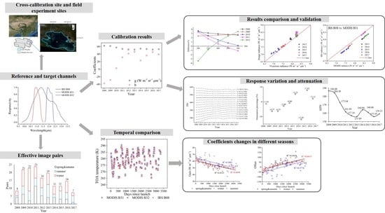
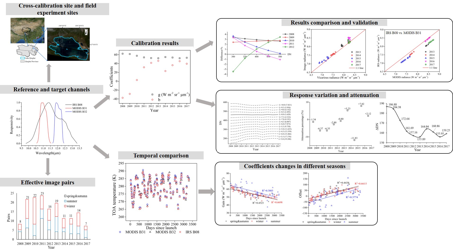
Orbital Lifetime (2008–2017) Radiometric Calibration and Evaluation of the HJ-1B IRS Thermal Infrared Band

Abstract

The infrared sensor (IRS) is a payload on the HJ-1B satellite and includes a thermal infrared band (B08). In order to obtain radiometric calibration coefficients and evaluate annual change, this study performed an analysis covering its 10-year orbital lifetime (2008–2017). The cross-calibration of IRS B08 with MODIS was performed using near-simultaneous images over Lake Qinghai, China. The results reveal that the radiometric response of IRS B08 notably changed during its orbital lifetime from year-to-year. The offsets fluctuated more than the gain. The top-of-atmosphere (TOA) radiance obtained by calibration coefficients in this study was generally in agreement with those obtained by onboard calibrator, within an error range of ±4.00% from 2008 to 2012. The percent difference compared with field validation was within 1.63%. The difference between IRS and MODIS radiance over field validation sites was within ±5%. Approximately a 1% difference occurred between the TOA temperature of IRS and MODIS. The radiometric response of IRS B08 continuously decreased from 2008 to 2013, whereas it fluctuated from 2014 to 2017. Moreover, the DN fluctuated more when the at-aperture radiance was low, although it was more stable at higher radiance.

1. Introduction

Research utilizing derived thermal infrared data has become a hot topic in recent decades. The value of thermal data archives will continue to grow since they can be applied to many areas, such as the monitoring of evapotranspiration [1,2], the estimation of soil moisture [3], the detection of the geothermal system [4,5] and mineral mapping [6,7]. In order to take proper advantage of thermal infrared data, a critical step is radiometric calibration, which converts observed digital numbers (DNs) to physical radiance quantities [8]. One of the virtual purposes of this process is to provide calibration coefficients to consistently convert DNs into top-of-atmosphere (TOA) radiances. The converted radiance that explicitly embodies the reflective or emissive properties from the terrestrial surface is usually taken as the most important preliminary input in quantitative applications.

In general, there are four main methods used to obtain calibration coefficients: preflight calibration, in-flight calibration, vicarious calibration and cross-calibration. Since the in-orbit environment differs from the simulated environment in the laboratory, post-flight calibration is required even if the preflight calibration is performed perfectly [9]. Meanwhile, in-flight calibration is heavily dependent upon the onboard calibration systems. Vicarious calibration requires a large amount of simultaneous data and its cost is usually high [10]. In addition, it cannot be used to calibrate historical data. Comparatively speaking, cross-calibration is a more flexible and economic way to obtain calibration coefficients, especially for historical data [11,12,13,14,15].

The HJ-1 constellation contains two optical satellites (HJ-1A and HJ-1B) and a radar satellite (HJ-1C). It was launched on September 6, 2008, with the specific objective of obtaining data that could be used for environmental protection and disaster reduction in China. The life expectancy of IRS was only three years, but it has now provided records of the Earth’s surface for more than a decade [16,17]. The payloads on the HJ-IB contain a 4-band charge-coupled device (CCD) and another 4-band infrared sensor (IRS), including a thermal infrared band (B08). The spectral range of IRS B08 is 10.5–12.5 μm, and the spatial resolution is 300 m. The IRS has a high temporal resolution (every four days) and its images are freely available to the public. The sea surface temperature (SST) [18] and land surface temperature (LST) [19,20] can be retrieved from the IRS B08. The retrieved SSTs from the IRS are within the acceptable range. The improved mono-window algorithm for retrieving LST established by Zhou et al. [19] is applicable and feasible in actual conditions when compared to MODIS LST products. Given these advantages, the data are more suitable for eco-environment monitoring in near real time than Landsat as well as assessment accuracy than MODIS. Examples include the detection of urban heat islands [21,22,23,24], the monitoring of abnormal thermal points [25,26], the mapping of urban land cover [27], the monitoring of water bodies [28]. Wong et al. [21] developed a novel algorithm to estimate anthropogenic heat fluxes using HJ-1B images. Their method can help in the understanding of the anthropogenic heat flux relationship with and formation of the urban heat islands effect. Wu et al. [24] utilized various biophysical indices, such as NDVI, landscape metrics, to test the performance of the HJ-1B thermal infrared band in the monitoring of urban heat islands. Their findings revealed the impacts of the spatial structure of land use on urban heat islands, which is helpful for improving the planning and management of the urban environment. A spatiotemporal model established by Lin et al. using HJ-1B/IRS images performed better for background brightness temperature prediction during the fire season when compared to the contextual algorithm. HJ-1B images can be used to improve the classification accuracies of detailed urban land–cover mapping [27]. However, those studies are mainly focused on the images before 2013, the images acquired after 2013 are not fully used due to the lack of radiometric calibration coefficients.

Since the launch of HJ-1 constellation, the instrument response of the thermal infrared band has changed over time [14,29]. In addition, it may be affected by various uncertainty factors, such as straylight [30,31]. Accordingly, its in-orbit radiometric characteristics have inevitably deviated from those designed in the pre-launch laboratory. Therefore, radiometric calibration and evaluation on an annual basis are required for utilization of the IRS data. The China Center for Resource Satellite Data and Application (CCRSDA) was responsible for updating the IRS radiometric calibration coefficients from 2008 to 2012. Regrettably, the CCRSDA ended this updating in 2013 due to the loss of on-board calibration ability, although the IRS continued its in-orbit function for the next five years through 2017. Here, in order to improve the accuracy and usefulness of the application of IRS images and to compensate for the lack of radiometric calibration coefficients, we performed cross-calibration of the IRS B08 with moderate-resolution imaging spectroradiometer (MODIS) B31 and B32 over 10 year- period (2008–2017). Furthermore, we also analyzed the instrument response variation over its entire orbital lifetime, with the expectation of discovering the detector’s decay characteristics.

2. Materials and Methods

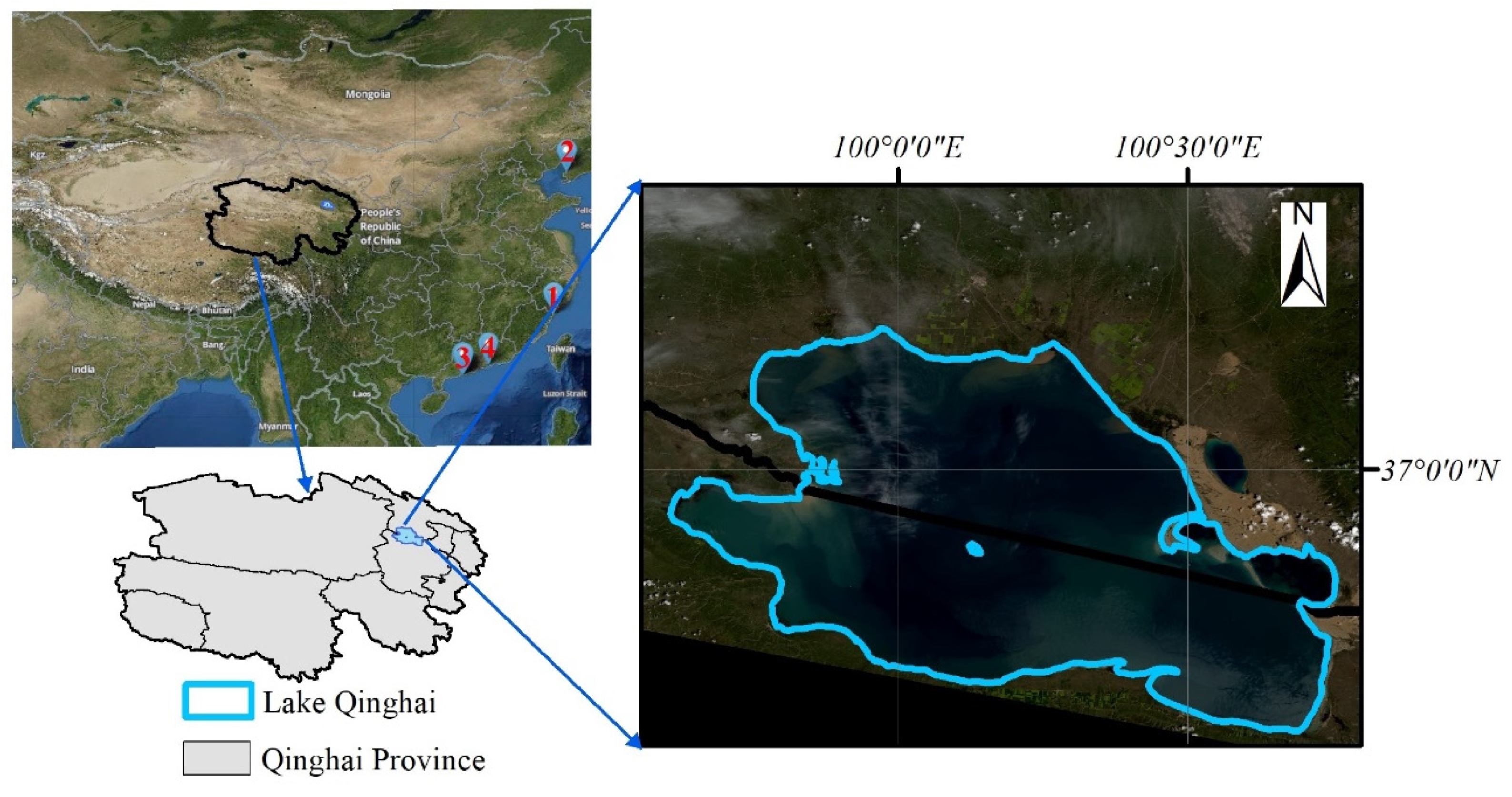
2.1. Study Areas and Data Sources

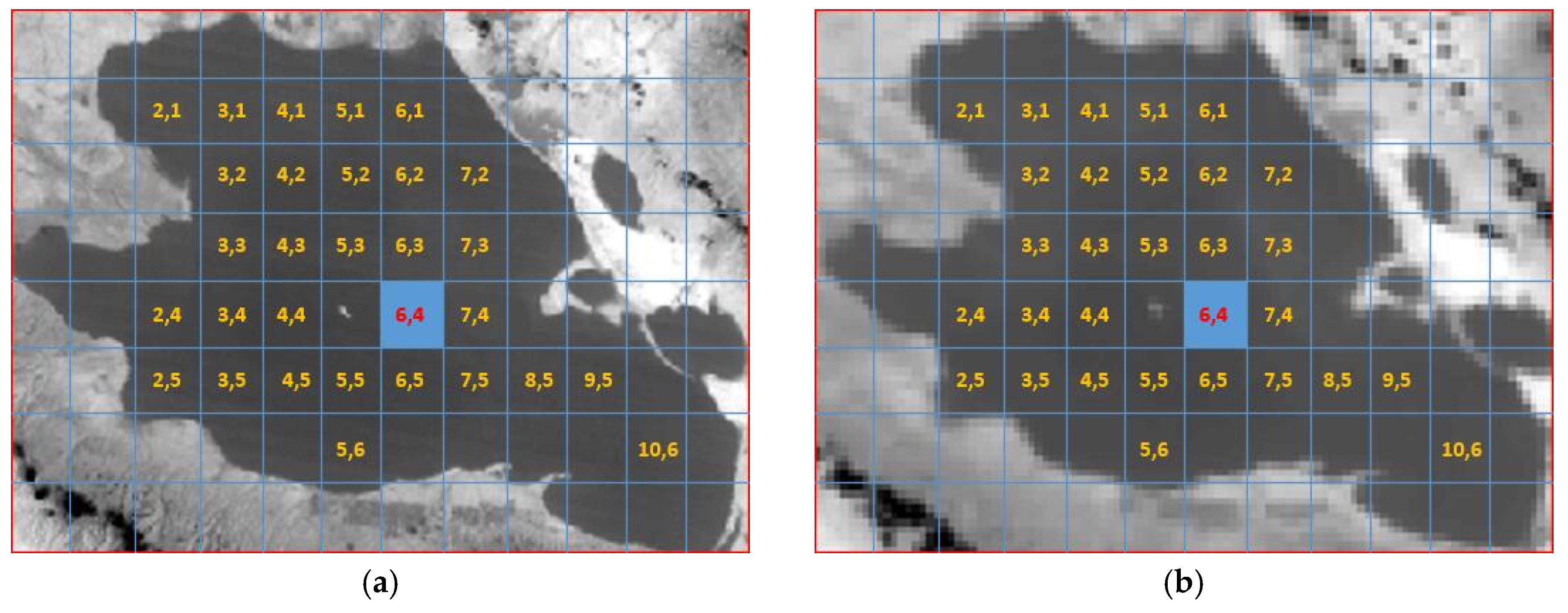
2.1.1. Cross-Calibration Site

Water is an ideal target for thermal infrared calibration, given its high emissivity and low surface temperature variation across large areas over short time spans. Lake Qinghai (Figure 1) located between 36°32′~37°15′ N, 99°36′~100°16′ E, is the largest inland saltwater lake in China. It has an area of 4473 km² and a maximum depth of 32.8 m. The surface elevation is 3196 m above sea level, and the atmosphere above the site is typically dry and stable with low amounts of total water vapor content in the atmospheric column. The surface temperature is uniform, with a horizontal surface temperature gradient <0.12 °C. Hence, the water body is a natural infrared radiation target. According to Wan et al. [32,33], Lake Qinghai is one of the primary thermal infrared calibration fields in China, and is widely used in satellite in-orbit radiometric calibration.

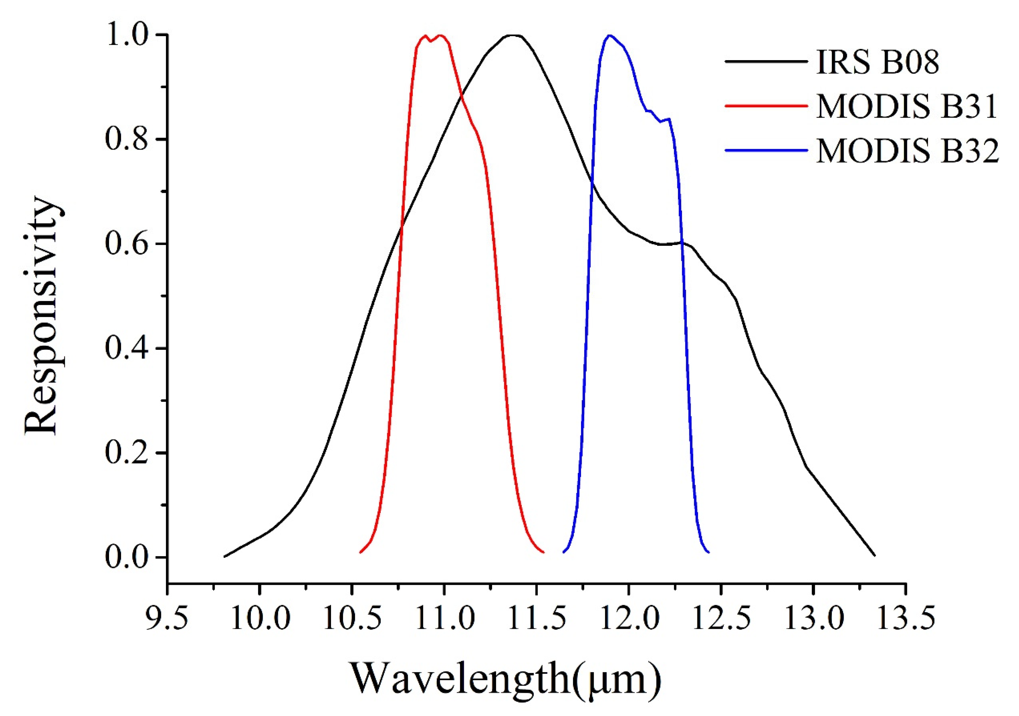
2.1.2. Reference Data

The cross-calibration method requires relatively high calibration accuracy of the reference sensor. The MODIS is an important sensor on the Terra that observes the Earth’s surface every 1–2 days. The MODIS instrument has 36 bands, and its thermal infrared (TIR) range is 3–15μm. MODIS band 31 (10.78–11.28 μm) and band 32 (11.77–12.27 μm) overlapped with IRS band 08 (10.50–12.50 μm); a comparison of their channel response functions is presented in Figure 2. In addition, the MODIS TIR bands are perfectly calibrated through the onboard blackbody, and the uncertainty of absolute radiometric accuracy for bands 31 and 32 is 2% [33,34]. Since both are morning satellites the pass time difference between the Terra and the HJ-1B over Lake Qinghai is about 1 h—and sometimes only a few minutes. Therefore, this study selected MODIS B31 and B32 as the reference channels for the IRS B08 cross-calibration.

Table 1. Comparison of selected thermal band features of the infrared sensor (IRS) and moderate-resolution imaging spectroradiometer (MODIS).

	Band Pass (μm)	Spatial Resolution (m)	Signal Quantization Levels (bits)	NEΔT (K)
IRS B08	10.50–12.50	300	10	0.38
MODIS B31	10.78–11.28	1000	12	0.05
MODIS B32	11.77–12.27	1000	12	0.05

compares the thermal band features of both instruments.

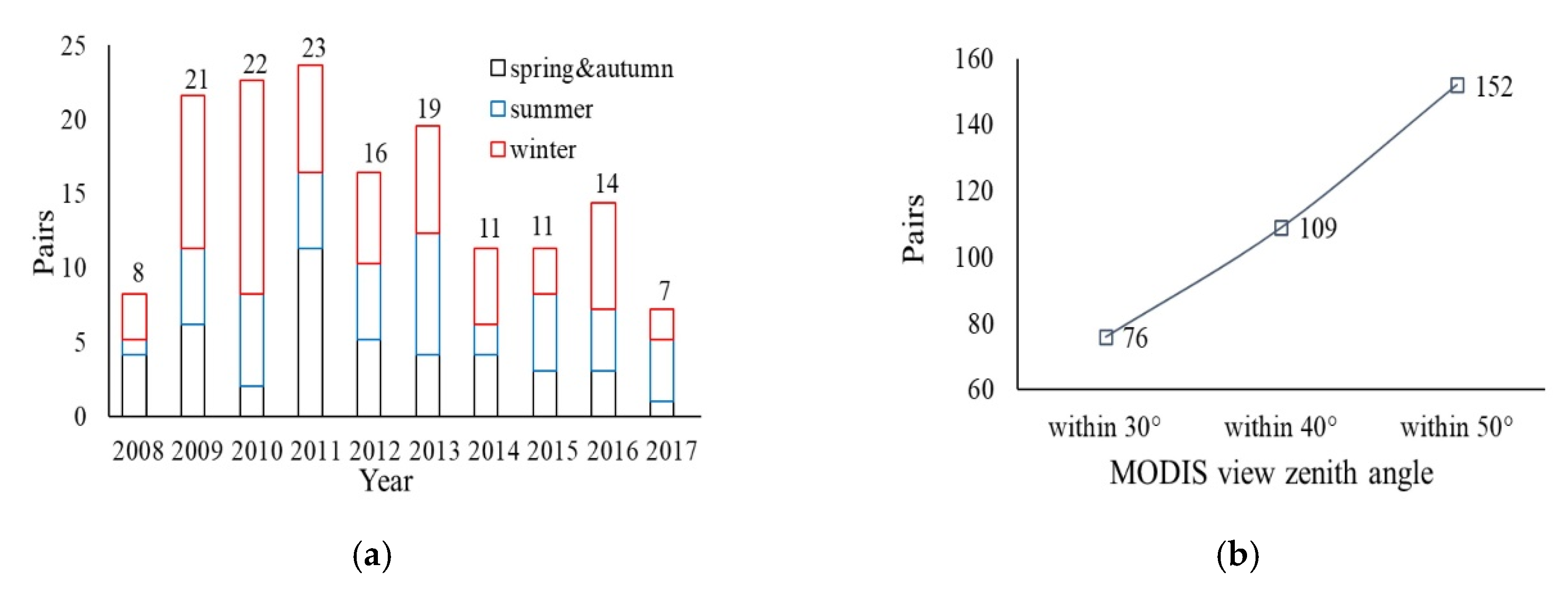
2.1.3. Image Pairs Matching and Statistics

Near-simultaneous IRS and MODIS images over Lake Qinghai were selected and matched as one-to-one experimental data pairs. Excluding images dominated by cloud or ice, 208 image pairs were chosen. Based on the accuracy distribution characteristics of the twin-channel difference model used in this study (introduced in the section below), 56 pairs with MODIS-view zenith angles >50° were discarded. The remaining 152 pairs were then used to perform the radiometric calibration. The images pairs were further subdivided into three groups based on their corresponding MODIS-view zenith angle, i.e., within 30°, within 40° and within 50°. The annual effective data volumes are graphed in Figure 3a and the distribution of the MODIS-view zenith angle is plotted in Figure 3b.

2.2. Methods

2.2.1. Image Preprocessing

Image preprocessing includes fine geometric correction and resampling. The Landsat thematic mapper (TM) image orthorectification method has been successfully employed. Therefore, the IRS and MODIS images were geometrically corrected based on the fine geometric correction data of the Landsat TM (LT05_L1TP_133034_20070822). Since the spatial resolution of IRS B08 is 300 m but are 1 km for MODIS B31 and B32 bands, IRS B08 data were resampled to MODIS 1 km resolution using cubic convolution.

A uniform and stable subarea on the lake is the preferable region of interest (ROI) for performing cross-calibration. During the selection of the ROI, the lake surface was gridded into approximate 20 km × 20 km squares [15], as illustrated in Figure 4. The squares containing both water and land were discarded in order to ensure feature uniformity in the target area. Each square labeled with row and column numbers in Figure 4 was iterated in order to mask and extract the radiance from MODIS B31 and B32, after which the radiance variance was calculated for each. The blue grid (6, 4) in Figure 4 corresponds to the smallest variance, indicating that the average thermal radiative characteristics in this grid are more uniform and stable than those in other grids. Therefore, this grid square was selected as the final ROI used to perform radiometric cross-calibration in this study.

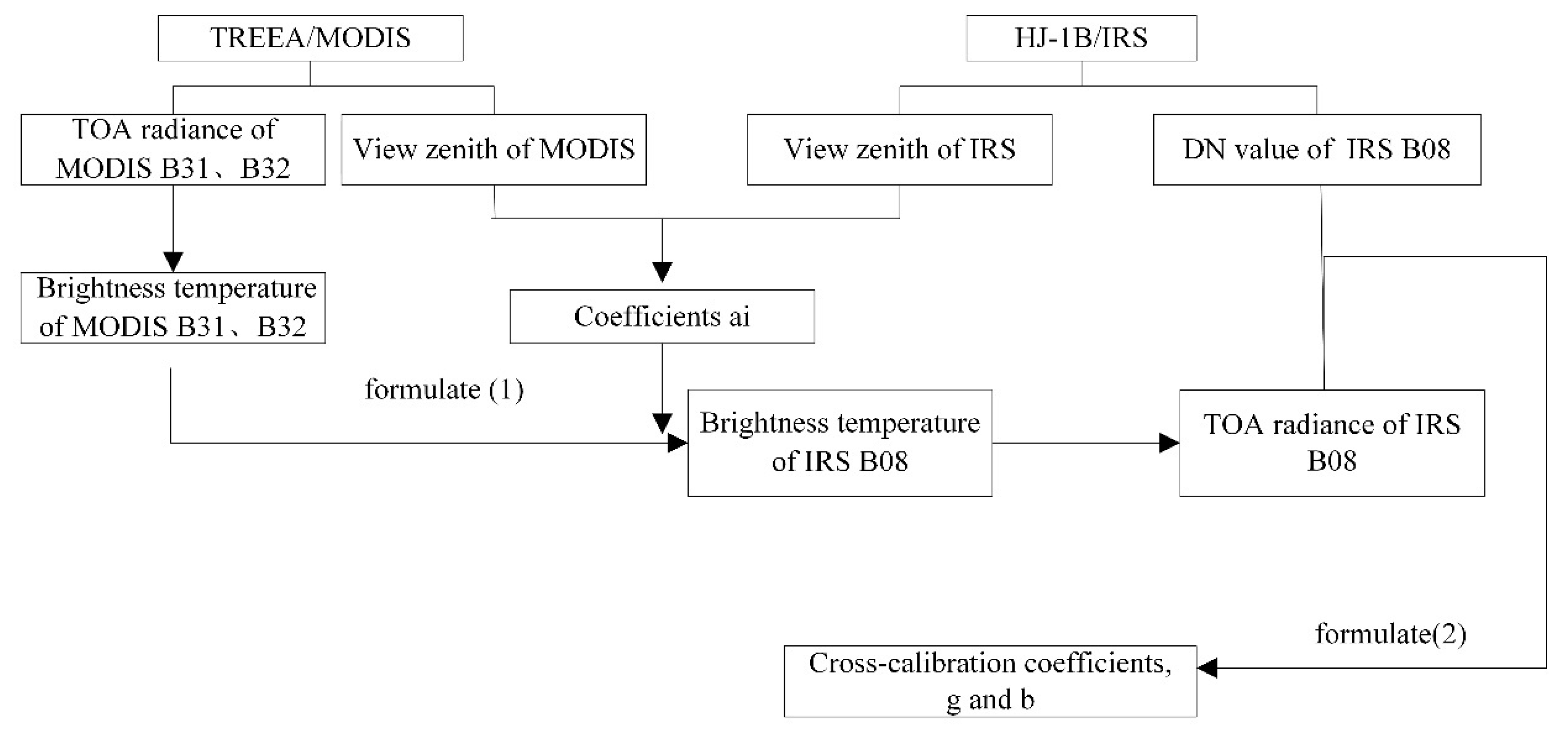
2.2.2. TOA Radiance Calibration and Coefficients Regression

The twin-channel difference model, which is a simplified physical model, was established based on radiative transfer model [16]. This model can avoid the effects of atmospheric temperature and density on the calibration process without additional observation parameters and is an ideal high-frequency and high-precision calibration algorithm for in-orbit sensors. Therefore, it was applied here to cross calibrate the IRS B08 with the MODIS B31 and B32.

The model is expressed by different combination of the TOA temperature of reference channels, as:

$${\mathrm{T}}_{\mathrm{H}08}={\mathrm{a}}_1+{\mathrm{a}}_2·{\mathrm{T}}_{\mathrm{M}31}+{\mathrm{a}}_3·\left({\mathrm{T}}_{\mathrm{M}32}-{\mathrm{T}}_{\mathrm{M}31}\right),$$

(1)

where ${\mathrm{T}}_{\mathrm{H}08}$ is the TOA temperature of IRS B08 and ${\mathrm{T}}_{\mathrm{M}31}$, ${\mathrm{T}}_{\mathrm{M}32}$ are the TOA temperatures of MODIS B31, B32, respectively. The coefficients ${\mathrm{a}}_1$, ${\mathrm{a}}_2$, ${\mathrm{a}}_3$ can be obtained from the cross coefficients’ lookup table with corresponding observed geometric conditions.

Figure 5 illustrates the entire process for deducing radiometric coefficients via cross-calibration. The four main steps are described below.

• Obtain the DN of IRS B08, the radiance of MODIS B31 and B32 and the view zenith angles of ROI area from near-simultaneous image pairs;
• Convert the TOA radiance of MODIS B31, B32 into TOA temperature according to “temperature-radiance” lookup table and obtain cross coefficients, ${\mathrm{a}}_{\mathrm{i}}$, according to “cross coefficient” lookup table;
• Calculate the TOA temperature of IRS B08 using Equation (1) and convert to TOA radiance through the inverse of the Planck function or the “temperature-radiance” lookup table.
• Perform coefficients regression. The data obtained from the above process (DN and TOA radiance of IRS B08) were regressed using a linear equation as:

  $$\mathrm{L}=\frac{\mathrm{DN}-\mathrm{b}}{\mathrm{g}}$$

  (2)

  where $\mathrm{DN}$ is the digital number, $\mathrm{L}$ is TOA radiance, and $\mathrm{b}$ and $\mathrm{g}$ are the radiometric calibration coefficients of the expected offset and gain, respectively. The unit of $\mathrm{g}$ is ${\mathrm{W}}^{-1}·{\mathrm{m}}^2·\mathrm{s}\mathrm{r}·\mathsf{\mu }\mathrm{m}$, and $\mathrm{b}$ is unitless.

2.2.3. Field Experiment

The field validation techniques estimated the TOA radiance over a selected test site. Next, the simulated radiance was convolved with the relative channel spectral response function to obtain the predicted radiance at sensor. Finally, the predicted radiance at sensor was compared with the measured radiance. The TOA radiance values were simulated with the help of the radiation propagation code MODTRAN [35] using field measurements as inputs. Measured radiance was tested with a Cimel CE312 radiometer, which was accurately calibrated by a highly accurate field portable blackbody (Mikron M340) before and after the satellite overpass. Water was used as the target. The experiment was conducted concurrent with the satellite transit time.

The temperature-based method for radiation propagation to the sensor can be expressed as:

$${\mathrm{L}}_{\mathrm{TOA}}=\mathsf{\tau }·\frac{{\displaystyle \int }[\mathsf{\epsilon }\left(\mathsf{\lambda }\right)\mathrm{B}\left(\mathsf{\lambda },\mathrm{T}\right)+\left(1-\mathsf{\epsilon }\left(\mathsf{\lambda }\right)\right){\mathrm{L}}^{\downarrow }\left(\mathsf{\lambda }\right)]\mathrm{R}\left(\mathsf{\lambda }\right)\mathrm{d}\mathsf{\lambda }}{{\displaystyle \int }\mathrm{R}\left(\mathsf{\lambda }\right)\mathrm{d}\mathsf{\lambda }}+{\mathrm{L}}^{\uparrow }={\mathsf{\tau }\mathrm{L}}_{\mathrm{obs}}+{\mathrm{L}}^{\uparrow }$$

(3)

where ${\mathrm{L}}_{\mathrm{TOA}}$ is the TOA radiance, $\mathsf{\tau }$ is the atmospheric transmittance from ground to sensor, $\mathsf{\epsilon }\left(\mathsf{\lambda }\right)$ is the spectral emissivity of the observed target, $\mathrm{B}\left(\mathsf{\lambda },\mathrm{T}\right)$ is the Planck function associated with a target at temperature $\mathrm{T}$, ${\mathrm{L}}^{\downarrow }\left(\mathsf{\lambda }\right)$ is the spectral downwelling radiance, ${\mathrm{L}}^{\uparrow }\left(\mathsf{\lambda }\right)$ is the channel upwelling radiance, $\mathrm{R}\left(\mathsf{\lambda }\right)$ is the relative channel spectral response function of the sensor (IRS in this study) and ${\mathrm{L}}_{\mathrm{obs}}$ is the channel radiance assuming the sensor was located on the ground.

In the radiance-based method, ${\mathrm{L}}_{\mathrm{obs}}$ is calculated using Equation (4):

$${\mathrm{L}}_{\mathrm{obs}}=\frac{{\mathsf{\epsilon }}_{\mathrm{obs}}\mathrm{B}\left({\mathsf{\lambda }}_{\mathrm{obs}},\mathrm{T}\right)+\left(1-{\mathsf{\epsilon }}_{\mathrm{obs}}\right){\mathrm{L}}^{\downarrow }}{{\mathsf{\epsilon }}_{\mathrm{M}}\mathrm{B}\left({\mathsf{\lambda }}_{\mathrm{M}},\mathrm{T}\right)+\left(1-{\mathsf{\epsilon }}_{\mathrm{M}}\right){\mathrm{L}}_{\mathrm{M}}^{\downarrow }}·{\mathrm{L}}_{\mathrm{M}}$$

(4)

where $\mathrm{M}$ is the parameter that corresponds to the ground instrument (the Cimel CE312 in this study).

The atmospheric profile data used by MODTRAN to simulate $\mathsf{\tau }$, ${\mathrm{L}}^{\uparrow }$ and ${\mathrm{L}}^{\downarrow }$ were from atmospheric sounding balloons.

The field experiment sites used for this study are listed in

Table 2. Field experiment information (* Numbers correspond to Figure 1).

Number *	Date	Site	Longitude	Latitude
1	26 October 2013	Ningde, China	120.31° E	27.04° N
2	12 June 2014	Hongyanhe, China	121.46° E	39.78° N
3	28 January 2015	Yangjiang, China	112.17° E	21.42° N
4	14 October 2016	Daya Bay, China	114.32° E	22.36° N
4	21 October 2017	Daya Bay, China	114.32° E	22.36° N

. They are distributed in the southeast coastal area of China, from temperate to subtropical. The tested water temperature ranged from 280 to 295 K.

3. Results

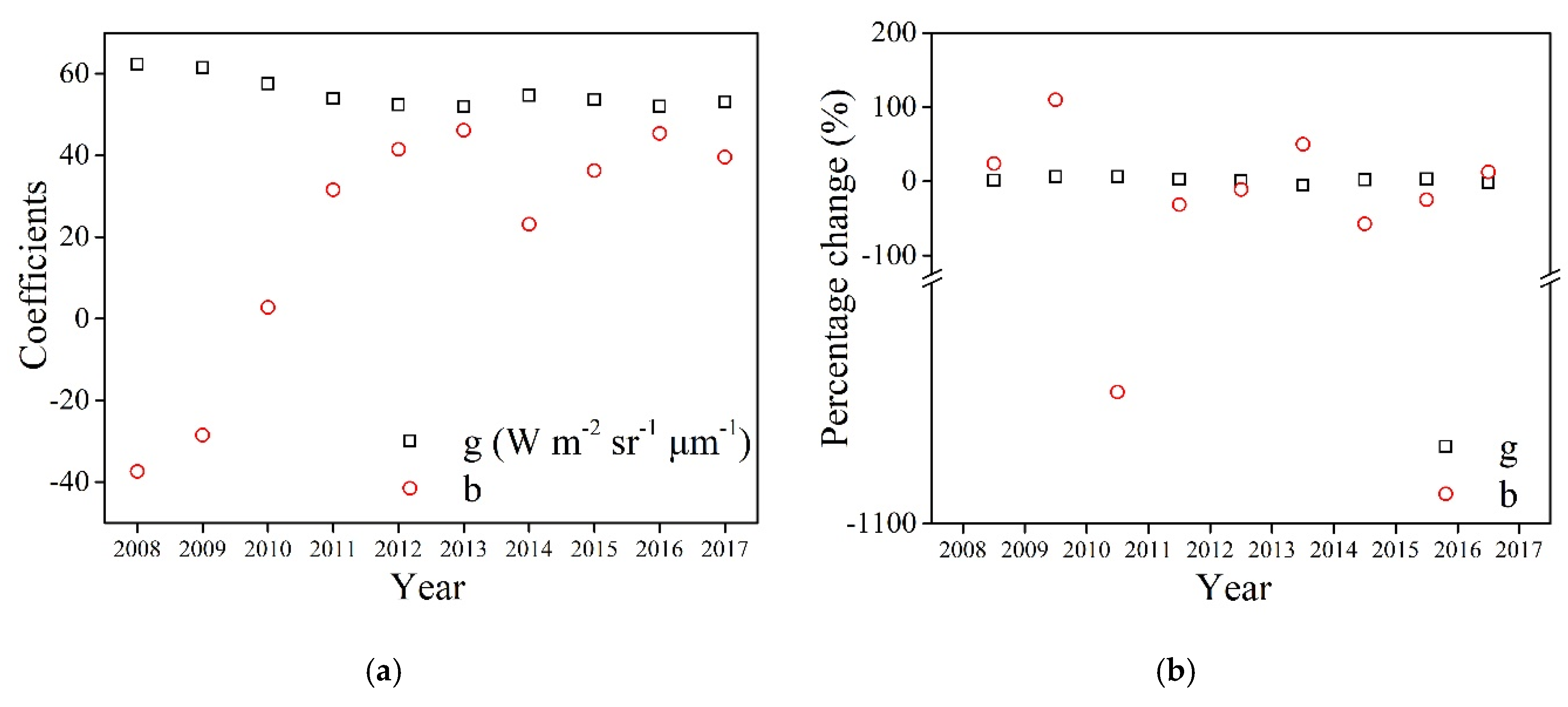
3.1. Annual Calibration Coefficients

The radiometric calibration coefficients of the IRS B08 from 2008 to 2017 obtained in this study are listed in

Table 3. Radiometric calibration coefficients of IRS B08 from 2008 to 2017.

Cross-Calibration Coefficients				Official Coefficients
Year	g ($W^{-1}·m^2·sr·\mathsf{\mu }m$)	b	R2	g ($W^{-1}·m^2·sr·\mathsf{\mu }m$)	b
2008	62.293	−37.409	0.9781	61.472	−44.598
2009	61.460	−28.509	0.9937	59.421	−25.441
2010	57.548	2.755	0.9951	60.713	−25.441
2011	53.896	31.557	0.9916	56.277	12.626
2012	52.385	41.471	0.9817	47.744	70.185
2013	51.964	46.128	0.9891
2014	54.680	23.084	0.9753
2015	53.619	36.294	0.9865
2016	51.983	45.359	0.9913
2017	53.084	39.602	0.9875

, while, the official coefficients provided by the CCRSDA from 2008 to 2012 are listed in Table 3.

Figure 6a,b presents the numeric values and percent changes of gains and offsets from 2008 to 2017. The mean value of the gains was 55.176 ${\mathrm{W}}^{-1}·{\mathrm{m}}^2·\mathrm{sr}·\mathsf{\mu }\mathrm{m}$ and the percent changes were within $\pm$6.5%. The fluctuations of the offsets were greater than those of the gains, however.

3.2. Coefficients Validation

3.2.1. On-board Validation

The official coefficients were obtained by on-board calibrators, which were used to validate the calibration results obtained in this study. The DNs of water in the images were approximately 400, with most ranging from 300 to 500. The radiance differences between the results obtained from the official coefficients and this study are shown in Figure 7. It can be seen that all the percent differences of radiance were within $\pm$4.00%. The best fitting result exhibited a 0.16% difference, while the worst fitting result was −3.64%. These results indicate that the cross-calibration coefficients calculated in this study are reliable.

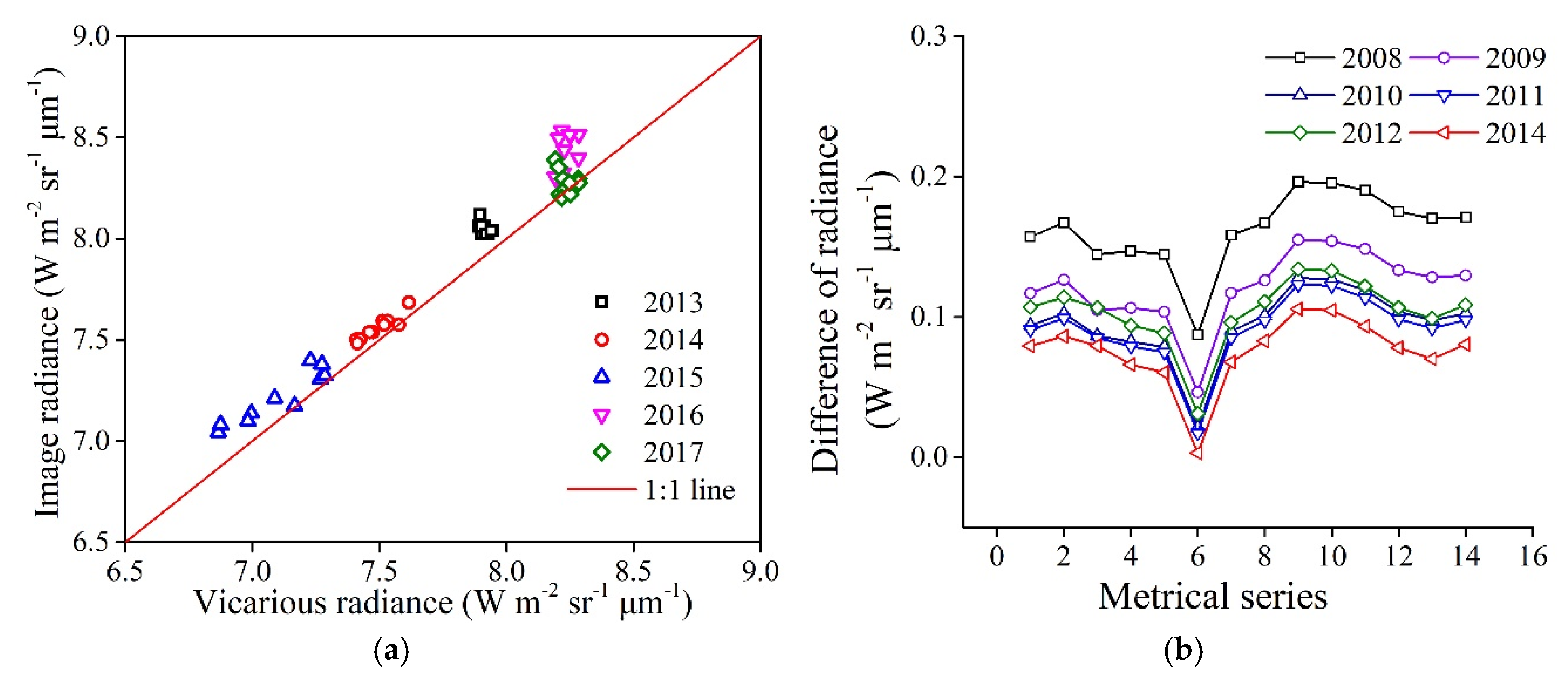
3.2.2. Vicarious Comparison

Based on the field experiments, the TOA radiance was simulated with the help of MODTRAN. The comparison of the radiance calculated using the cross-calibration coefficients and the field campaign measurements is presented in Figure 8a. They were close to the 1:1 line and the total error was within 0.11 $\mathrm{W}·{\mathrm{m}}^{-2}·{\mathrm{sr}}^{-1}·{\mathsf{\mu }\mathrm{m}}^{-1}$, corresponding to approximately 1.0 K of TOA temperature. The percent difference was within 1.63%. The image in 2014 was also calibrated using the calibration coefficients of the past few years. The radiance differences comparison between the cross-calibration and the field campaign is plotted in Figure 8b. These results indicated that not only the accuracy of the calibration coefficients in this study was reliable, but also the performance of the sensor changed with time.

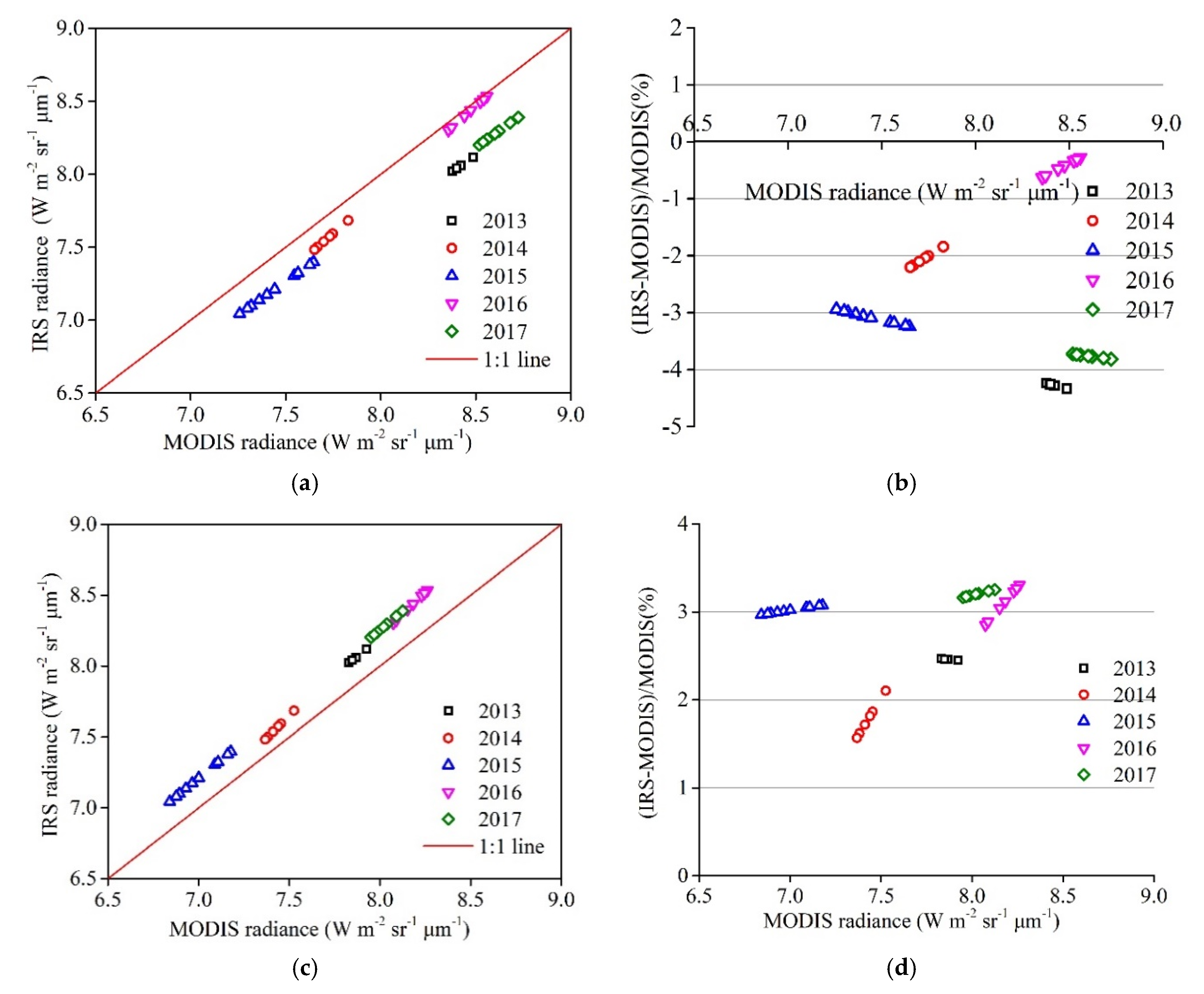
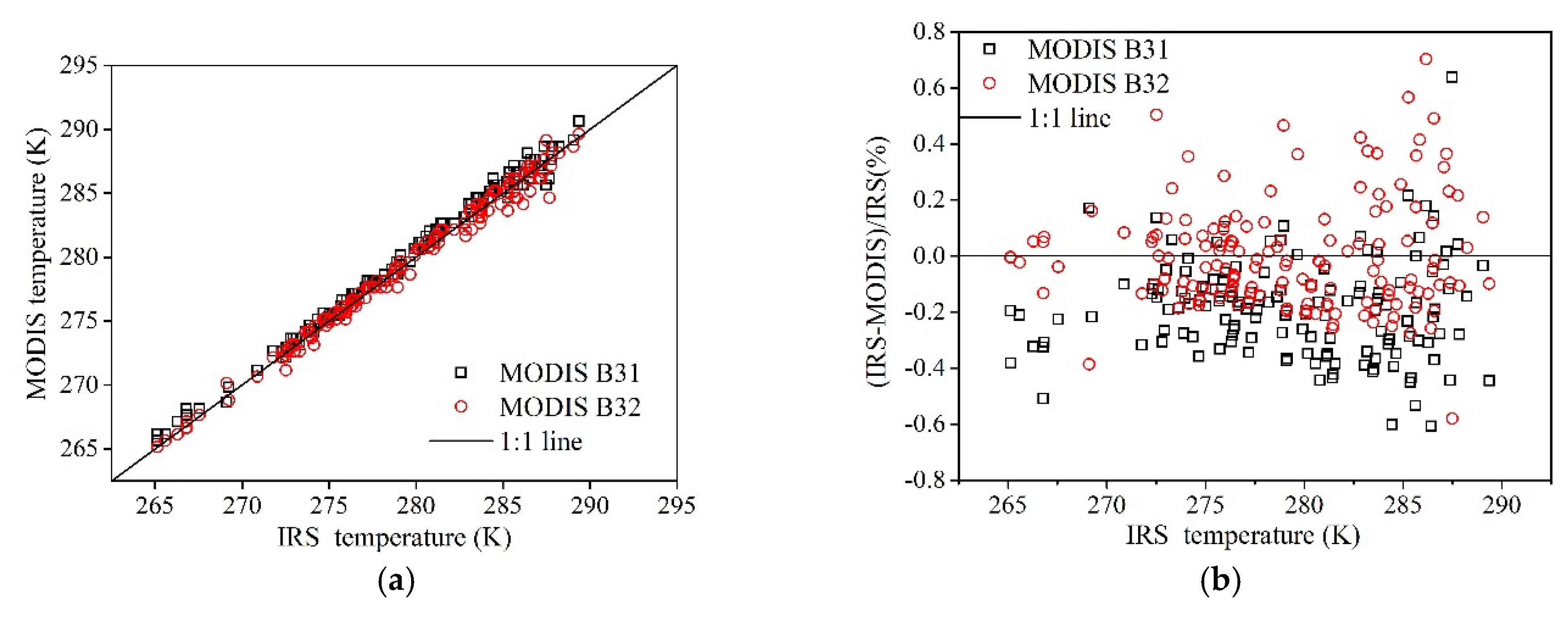
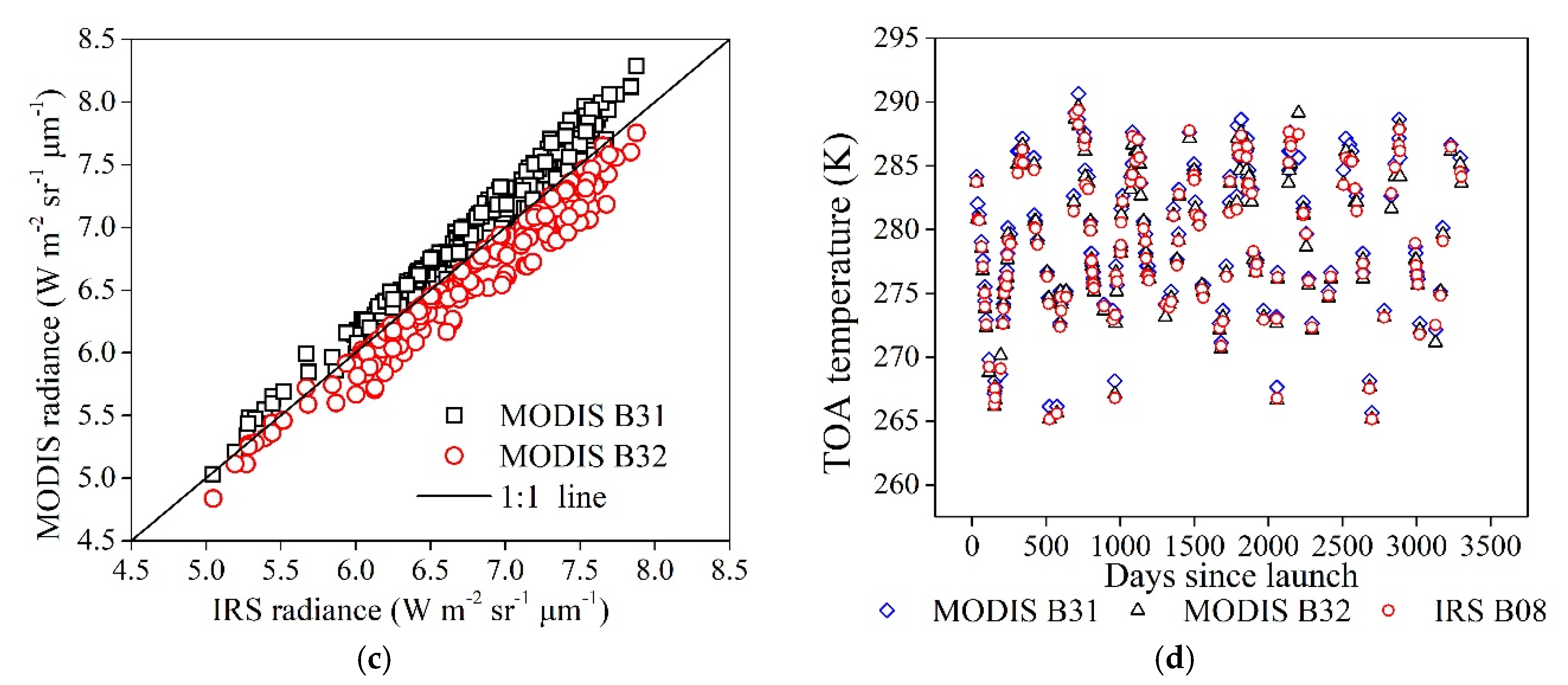
3.2.3. Image Cross-Comparison

The radiance obtained from images of the IRS B08 and the MODIS B31 and B32 over the field experiment sites was compared; the results from these comparisons are plotted in Figure 9. Each data point on the plots corresponds to a sampling points in the field experiments.

Figure 9a summarizes the radiance comparison results for the IRS B08 vs. MODIS B31. The data points do not lie precisely on the 1:1 line. In fact, all data points lie below the 1:1 line, indicating that IRS B08 was underestimating radiance in comparison to the MODIS B31. In the percent difference plots shown in Figure 9b, IRS B08 radiance estimates are as much as 5% lower. Figure 9c summarizes the radiance comparison results for the IRS B08 vs. MODIS B32. The percent difference plots presented in Figure 9d show that all data points lie above the zero line, indicating that the IRS B08 appears to estimate a 1% to 4% higher radiance than the MODIS B32.

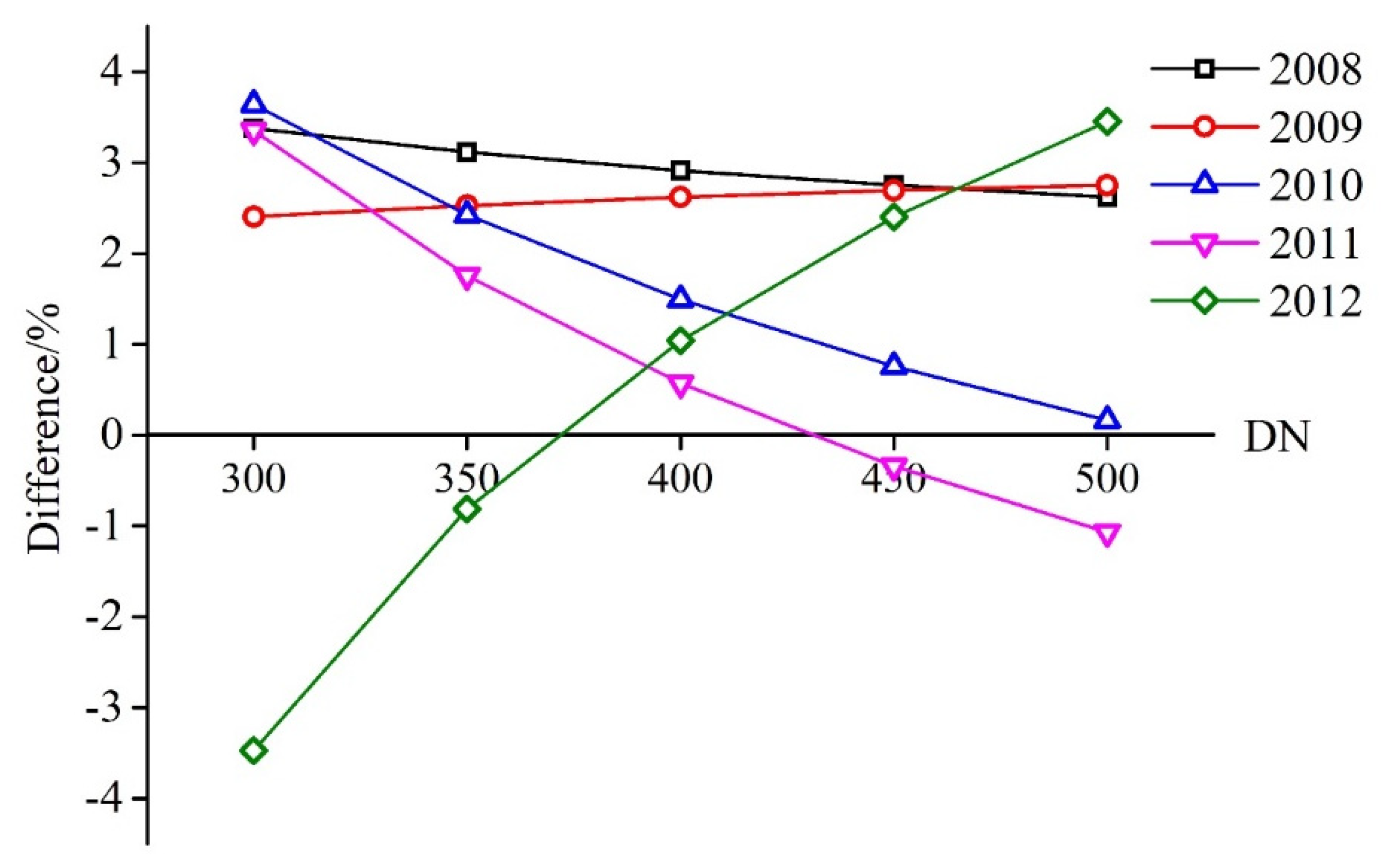
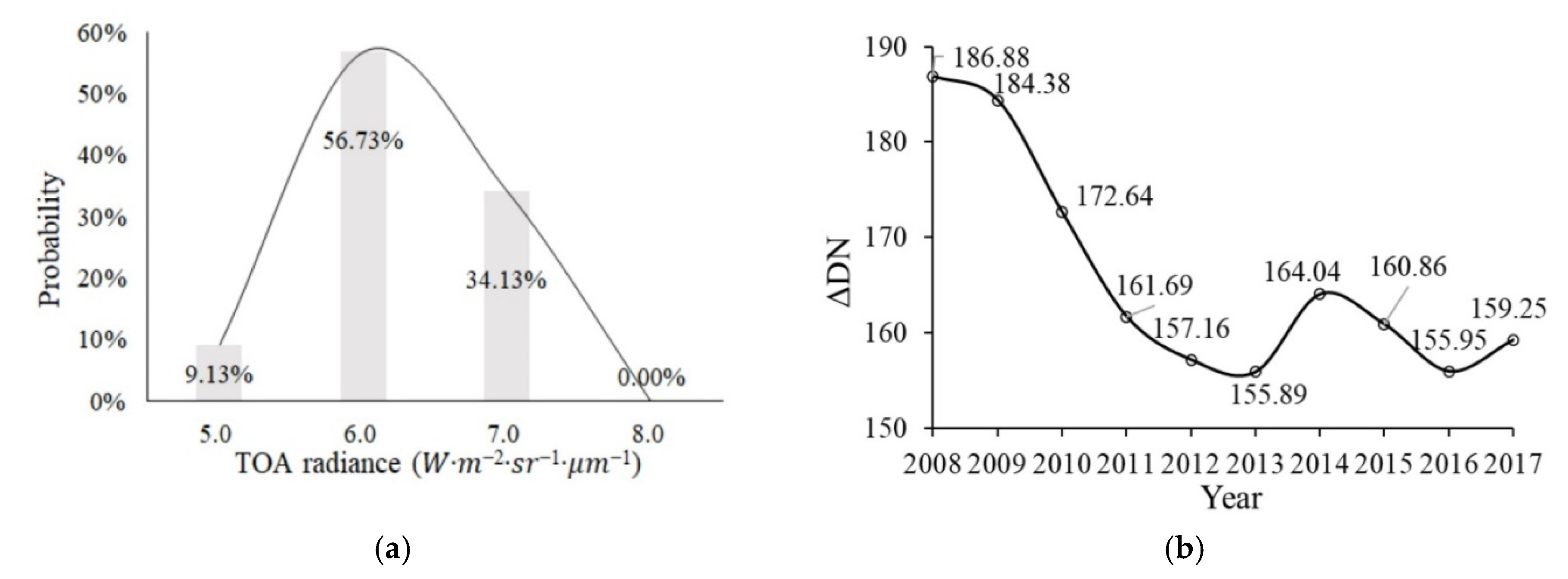
3.3. Relatively Low/Normal/High Radiance Variation

According to the applicable conditions of the twin-channel difference model, coefficients ${\mathrm{a}}_{\mathrm{i}}$ could be applied to all images in which the TOA temperature ranged from 240 to 310 K. When the temperature was 240 K, the corresponding radiance was approximately 3.0 $\mathrm{W}·{\mathrm{m}}^{-2}·{\mathrm{sr}}^{-1}·{\mathsf{\mu }\mathrm{m}}^{-1}$. When the temperature was 310 K, the corresponding radiance was approximately 10.0 $\mathrm{W}·{\mathrm{m}}^{-2}·{\mathrm{sr}}^{-1}·{\mathsf{\mu }\mathrm{m}}^{-1}$. The water DNs in the selected images were within 500, corresponding to an at-aperture radiation of approximately 8.5 $\mathrm{W}·{\mathrm{m}}^{-2}·{\mathrm{sr}}^{-1}·{\mathsf{\mu }\mathrm{m}}^{-1}$. The corresponding DN values from low radiance (3.0 $\mathrm{W}·{\mathrm{m}}^{-2}·{\mathrm{sr}}^{-1}·{\mathsf{\mu }\mathrm{m}}^{-1}$) to high radiance (10.0 $\mathrm{W}·{\mathrm{m}}^{-2}·{\mathrm{sr}}^{-1}·{\mathsf{\mu }\mathrm{m}}^{-1}$) were computed using the cross-calibration coefficients obtained in this study, and the results are presented in Figure 10. These results indicate that the DN at low radiance increased slightly from 2008 to 2013 and fluctuated after that time. It was more stable at normal radiance, however. When the radiance was 8.0 $\mathrm{W}·{\mathrm{m}}^{-2}·{\mathrm{sr}}^{-1}·{\mathsf{\mu }\mathrm{m}}^{-1}$, the corresponding DN was a nearly horizontal line from 2008 to 2017. The DN at the high radiance range decreased slightly from 2008 to 2013 and fluctuated from 2014 to 2017.

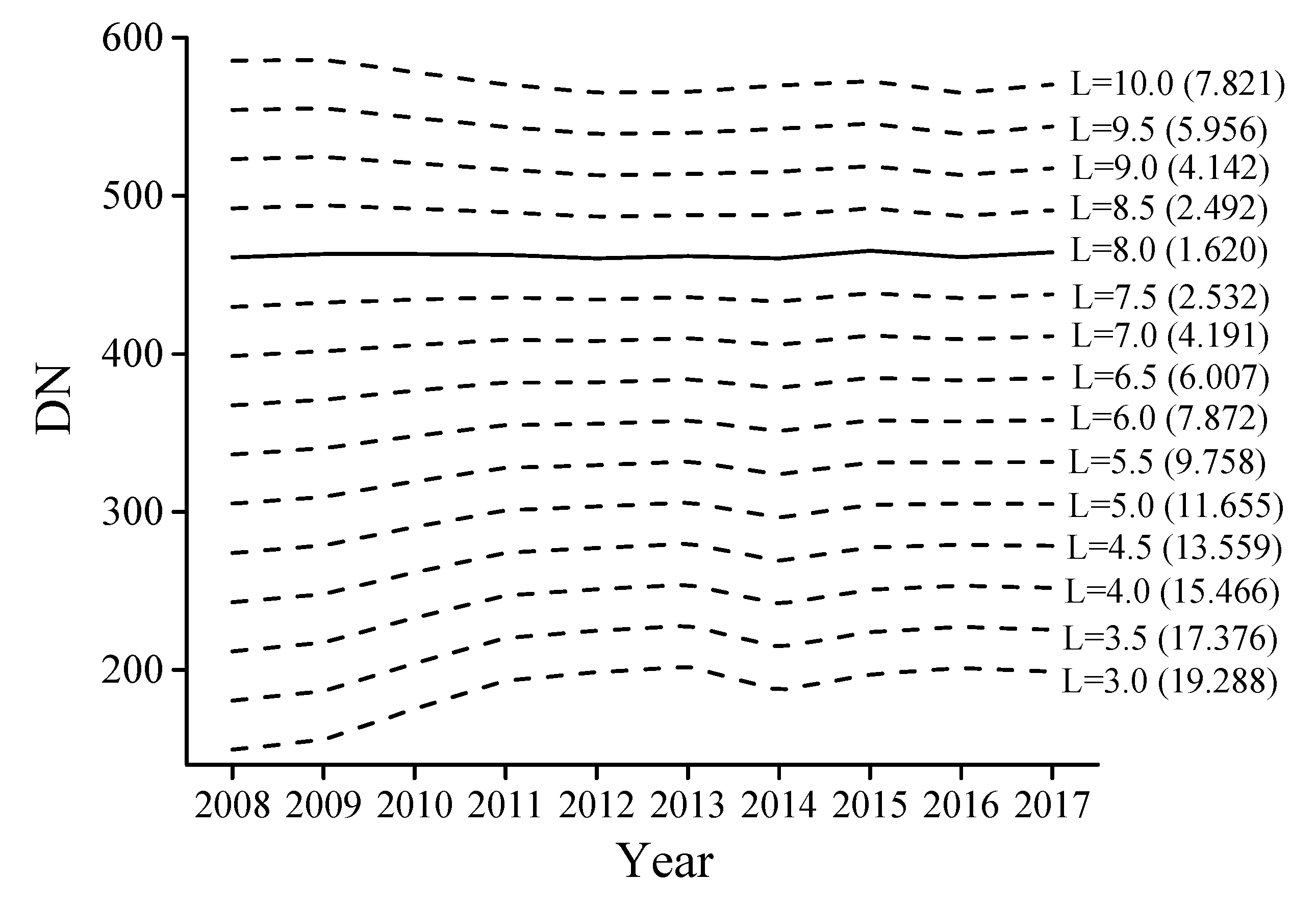
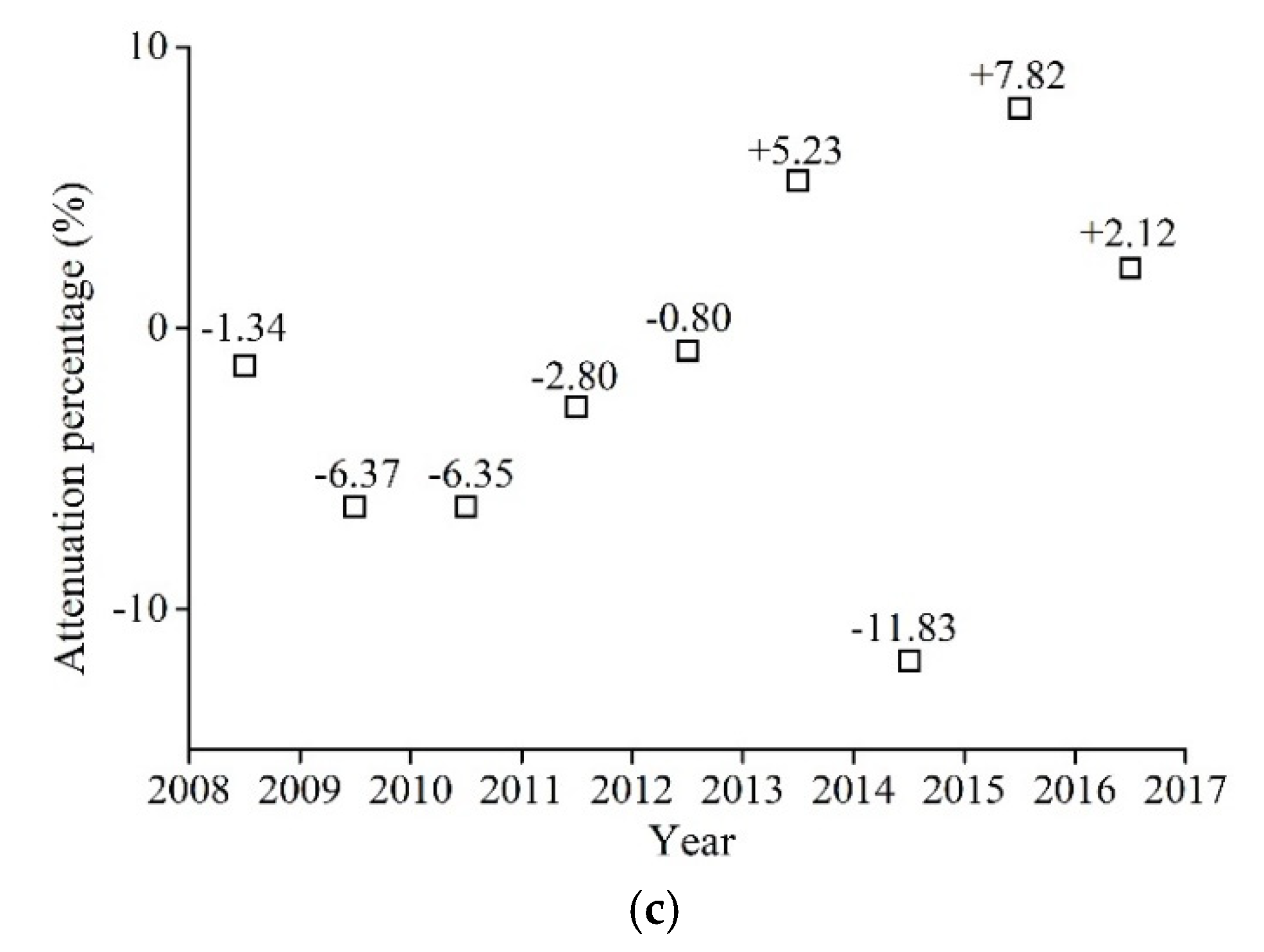
3.4. Channel Response Variation

As shown in Figure 11a, the TOA radiance range in the selected grids was 5.0–8.0 $\mathrm{W}·{\mathrm{m}}^{-2}·{\mathrm{sr}}^{-1}·{\mathsf{\mu }\mathrm{m}}^{-1}$. Therefore, we chose 5.0–8.0 $\mathrm{W}·{\mathrm{m}}^{-2}·{\mathrm{sr}}^{-1}·{\mathsf{\mu }\mathrm{m}}^{-1}$ as the input radiance interval to analyze the response of the sensor. The corresponding DNs were calculated with Equation (2) using the coefficients obtained in this study. The change in the DN range is presented in Figure 11b and the attenuation percentages are shown in Figure 11c. The larger the DN range, the higher the sensitivity of the sensor. It can clearly be seen from Figure 11 that the sensitivity of the sensor decreased year-by-year from 2008 to 2013, but fluctuated from 2014 to 2017.

In summary, the radiometric response of the IRS B08 changed significantly during its orbital lifetime. A negative number indicates that the radiometric response was lower than the previous year. In other words, under the same radiance input interval, the DN range became smaller. The radiometric response exhibited a downward trend year-by-year from 2009 to 2013, with the largest decrease occurring in 2010. The radiometric response increased by +5.23% in 2014, however and fluctuated after that time.

4. Discussion

Hundreds of near-simultaneous images of Lake Qinghai were collected from 2008 to 2017. This provided a long-term sequence of images for the thermal infrared cross-calibration of the instrument. Temperature linearization between the IRS B08 and MODIS B31 was performed before cross-calibration, as shown in Figure 12a. They manifested a very close linear correlation. All data points lie very near the 1:1 line, indicating excellent temperature agreement between the two sensors. The percent difference plots (Figure 12b) suggest a difference of approximately 1% relative to IRS. Generally, in Figure 12c, the MODIS B31 displays a higher radiance than the IRS B08, while the MODIS B32 has a lower radiance than the IRS B08. Radiance and temperature distribution as a function of the MODIS and IRS lifetimes are shown in Figure 12d. In different years, each channel exhibited sinusoidal trends. Therefore, they were effective in further analysis.

In Section 2.1.3, we discarded image pairs with zenith angles >50° in the MODIS view. We selected images from 2011 in order to verify the validity of this choice, since 2011 had the largest number of effective image pairs in this study. As shown in

Table 4. Fitting results of different MODIS-view zenith angles (2011).

Zenith	$\mathbf{g}({\mathbf{W}}^{-1}\mathbf{·}{\mathbf{m}}^2\mathbf{·}\mathbf{s}\mathbf{r}\mathbf{·}\mathsf{\mu }\mathbf{m})$	b	R2
Within 30°	54.142	29.944	0.9949
Within 40°	53.879	31.080	0.9938
Within 50°	53.896	31.557	0.9916
All angles	52.329	41.789	0.9792

, calibration accuracy is related to zenith angle. When images with a zenith angle > 50° were included, the worst fitting result occurred. Therefore, it was effective to filter the images based on the zenith angle of the MODIS view.

As described in Section 3.3, the radiometric response of the IRS B08 at normal at-aperture radiance was relatively stable. Therefore, we regarded it as a fixed regression point (L = 8.0 $\mathrm{W}·{\mathrm{m}}^{-2}·{\mathrm{sr}}^{-1}·{\mathsf{\mu }\mathrm{m}}^{-1}$, DN = 460). Combined with another point obtained by cross-calibration from each image pair, the linear regression coefficients could be calculated. The gains and offsets are shown in Figure 13a,b. Both gains and offsets were more dispersed in summer than in other seasons. The average surface temperature of Lake Qinghai in summer is approximately 289.15 K, and the highest temperature is 295.45 K, corresponding to the normal radiance range discussed in Section 3.3. The radiation response in this range was stable, so the gap between the DN and TOA radiation derived from MODIS in summer and the fixed point was relatively small. Therefore, the slope of the fitted line was small. A slight change in slope will cause a large change in the reciprocal, which is the gain. As a result, gains in summer exhibited more volatility. Correspondingly, the offsets also fluctuated more in summer than in other seasons. However, gains and offsets in winter were more stable, due to the fact that DN changed more when the temperature (radiance) was low.

Overall, the cross-calibration method is a cost-effective technique that is particularly tailored for long-term historical data. The attenuation characteristics of the sensor during its lifetime can be further analyzed based on the calibration coefficients. The coefficients of the IRS B08, especially from 2013 to 2017, provides an accurate guarantee for the quantitative application of IRS data. These data can be further applied to waterline extraction, temperature retrieval and other areas. The research results have fully enhanced the value of the HJ-1B satellite data.

5. Conclusions

Cross-calibration between the IRS B08 and MODIS B31, B32 was performed using near-simultaneous image pairs of Lake Qinghai over a 10-year lifetime (2008–2017). All images impacted by cloud or ice were discarded. In addition, since the calibration accuracy decreased significantly when images corresponding to MODIS zenith angles >50° were included, those images were excluded as well. The remaining 152 pairs were used to perform radiometric calibration. After various corrections, a very close linear correlation was found between the TOA radiances of IRS B08 and the DNs extracted from HJ-1B IRS images. The cross-calibration coefficients, gains and offsets, were obtained from 2008 to 2017, which compensated for the missing coefficients from 2013 to 2017. The percent difference was within ±4.00% when compared to the on-board calibrator results. Compared with the field campaign results, the percent difference was within 1.63%. The IRS B08 radiance is lower than that of MODIS B31 and higher than MODIS B32 radiance. However, the TOA temperature between the two sensors are highly consistent with approximately 1% difference. The calibration coefficients obtained in this study are highly accurate and can thus be used in the radiometric calibration of HJ-1B IRS images. The percent changes of gains were within $\pm$6.5%, although the percent changes of b were more scattered, indicating that the fluctuations of offsets were greater than those of gains. For the same radiance, the corresponding DN varied in different years. The DN values changed more in the low radiance range but were relatively stable in the normal radiance range. Therefore, the radiance in the normal range of L = 8.0 $\mathrm{W}·{\mathrm{m}}^{-2}·{\mathrm{sr}}^{-1}·{\mathsf{\mu }\mathrm{m}}^{-1}$ was regarded as a fixed point corresponding to DN = 460. Combined with another point obtained based on each image, cross-coefficients were calculated. The coefficients manifested different change characteristics in different seasons. The gain and offset values in summer were more volatile than in other seasons, while the winter values were the most stable. As a result, the DN range of the sensor differed for the same radiance input interval, meaning that the radiometric response of the IRS changed during its orbital lifetime. The response of the IRS decreased from 2008 to 2013 but fluctuated from 2014 to 2017.

With the calibration coefficients provided here, the IRS thermal archive calibrated the radiance to acceptable levels. SST and LST maps can be operationally produced from the IRS radiance data, and these data can also be used in various applications, such as waterline extraction, temperature retrieval and other research areas.

References

1. Du, T.; Yuan, G.; Wang, L.; Sun, X.; Sun, R. Comparison of Remotely Sensed Evapotranspiration Models Over Two Typical Sites in an Arid Riparian Ecosystem of Northwestern China. Remote Sens. 2020, 12, 1434. [Google Scholar] [CrossRef]
2. Anderson, M.C.; Kustas, W.P. Thermal Remote Sensing of Drought and Evapotranspiration. EOS Trans. 2008, 89, 233–234. [Google Scholar] [CrossRef]
3. Van Doninck, J.; Peters, J.; De Baets, B.; De Clercq, E.M.; Ducheyne, E.; Verhoest, N.E.C. The potential of multitemporal Aqua and Terra MODIS apparent thermal inertia as a soil moisture indicator. Int. J. Appl. Earth Obs. Geoinf. 2011, 13, 934–941. [Google Scholar] [CrossRef]
4. Van der Meer, F.; Hecker, C.; van Ruitenbeek, F.; van der Werff, H.; de Wijkerslooth, C.; Wechsler, C. Geologic remote sensing for geothermal exploration: A review. Int. J. Appl. Earth Obs. Geoinf. 2014, 33, 255–269. [Google Scholar] [CrossRef]
5. Romaguera, M.; Vaughan, R.G.; Ettema, J.; Izquierdo-Verdiguier, E.; Hecker, C.A.; van der Meer, F.D. Detecting geothermal anomalies and evaluating LST geothermal component by combining thermal remote sensing time series and land surface model data. Remote Sens. Environ. 2018, 204, 534–552. [Google Scholar] [CrossRef]
6. Ninomiya, Y.; Fu, B. Regional Lithological Mapping Using ASTER-TIR Data: Case Study for the Tibetan Plateau and the Surrounding Area. Geosciences 2016, 6, 39. [Google Scholar] [CrossRef] [Green Version]
7. Ninomiya, Y.; Fu, B. Thermal infrared multispectral remote sensing of lithology and mineralogy based on spectral properties of materials. Ore Geol. Rev. 2019, 108, 54–72. [Google Scholar] [CrossRef]
8. Tang, H.; Li, Z.L. Quantitative Remote Sensing in Thermal Infrared; Springer: Berlin/Heidelberg, Germany, 2014. [Google Scholar]
9. Thome, K.; Ara, K.; Hook, S.; Kieffer, H.; Lang, H.; Matsunaga, T.; Ono, A.; Palluconi, F.; Sakuma, H.; Slater, P.; et al. ASTER Preflight and Inflight Calibration and the Validation of Level 2 Products. IEEE Trans. Geosci. Remote Sens. 1998, 36, 1161–1172. [Google Scholar] [CrossRef]
10. Tonooka, H.; Palluconi, F.D.; Hook, S.J.; Matsunaga, T. Vicarious calibration of ASTER thermal infrared bands. IEEE Trans. Geosci. Remote Sens. 2005, 43, 2733–2746. [Google Scholar] [CrossRef]
11. Butler, J.J.; Choi, T.; Xiong, J.; Angal, A.; Chander, G.; Xiong, X. Radiometric cross-calibration of the Terra MODIS and Landsat 7 ETM+ using an invariant desert site. In Proceedings of the Earth Observing Systems XIII, San Diego, CA, USA, 11–13 August 2008. [Google Scholar]
12. Chander, G.; Angal, A.; Choi, T.; Xiong, X. Radiometric Cross-Calibration of EO-1 ALI with L7 ETM+ and Terra MODIS Sensors Using Near-Simultaneous Desert Observations. IEEE J. Sel. Top. Appl. Earth Obs. Remote Sens. 2013, 6, 386–399. [Google Scholar] [CrossRef]
13. Teillet, P.M.; Markham, B.L.; Irish, R.R. Landsat cross-calibration based on near simultaneous imaging of common ground targets. Remote Sens. Environ. 2006, 102, 264–270. [Google Scholar] [CrossRef] [Green Version]
14. Xiong, X.; Wenny, B.N.; Wu, A.; Barnes, W.L.; Salomonson, V.V. Aqua MODIS Thermal Emissive Band On-Orbit Calibration, Characterization, and Performance. IEEE Trans. Geosci. Remote Sens. 2009, 47, 803–814. [Google Scholar] [CrossRef] [Green Version]
15. Vermote, E.F.; Saleous, N.Z. Calibration of NOAA16 AVHRR over a desert site using MODIS data. Remote Sens. Environ. 2006, 105, 214–220. [Google Scholar] [CrossRef]
16. Li, J.; Gu, X.; Yu, T.; Li, X.; Gao, H.; Liu, L.; Xu, H. A twin-channel difference model for cross-calibration of thermal infrared band. Sci. China Technol. Sci. 2012, 55, 2048–2056. [Google Scholar] [CrossRef]
17. Wang, Q.; Wu, C.; Li, Q.; Li, J. Chinese HJ-1A/B satellites and data characteristics. Sci. China Earth Sci. 2011, 53, 51–57. [Google Scholar] [CrossRef]
18. Zhang, C.; Zhou, S.J.; Zhu, L. Three algorithms of sea surface temperature inversion of Daya Bay based on environmental star HJ_1B data. J. East China Inst. Technol. 2013, 36, 88–92. [Google Scholar]
19. Zhou, J.; Zhan, W.; Hu, D.; Zhao, X. Improvement of mono-window algorithm for retrieving land surface temperature from HJ-1B satellite data. Chin. Geogr. Sci. 2010, 20, 123–131. [Google Scholar] [CrossRef]
20. Ouyang, X.; Jia, L.; Pan, Y.; Hu, G. Retrieval of Land Surface Temperature over the Heihe River Basin Using HJ-1B Thermal Infrared Data. Remote Sens. 2014, 7, 300–318. [Google Scholar] [CrossRef] [Green Version]
21. Man Sing, W.; Jinxin, Y.; Nichol, J.; Qihao, W.; Menenti, M.; Chan, P.W. Modeling of Anthropogenic Heat Flux Using HJ-1B Chinese Small Satellite Image: A Study of Heterogeneous Urbanized Areas in Hong Kong. IEEE Geosci. Remote Sens. Lett. 2015, 12, 1466–1470. [Google Scholar] [CrossRef]
22. Yang, J.; Gong, P.; Zhou, J.; Huang, H.; Wang, L. Detection of the urban heat island in Beijing using HJ-1B satellite imagery. Sci. China Earth Sci. 2011, 53, 67–73. [Google Scholar] [CrossRef]
23. Sheng, L.; Lu, D.; Huang, J. Impacts of land-cover types on an urban heat island in Hangzhou, China. Int. J. Remote Sens. 2015, 36, 1584–1603. [Google Scholar] [CrossRef]
24. Wu, H.; Ye, L.P.; Shi, W.Z.; Clarke, K.C. Assessing the effects of land use spatial structure on urban heat islands using HJ-1B remote sensing imagery in Wuhan, China. Int. J. Appl. Earth Obs. Geoinf. 2014, 32, 67–78. [Google Scholar] [CrossRef]
25. Lin, L.; Meng, Y.; Yue, A.; Yuan, Y.; Liu, X.; Chen, J.; Zhang, M.; Chen, J. A Spatio-Temporal Model for Forest Fire Detection Using HJ-IRS Satellite Data. Remote Sens. 2016, 8, 403. [Google Scholar] [CrossRef] [Green Version]
26. Liu, W.; Wang, L.; Zhou, Y.; Wang, S.; Zhu, J.; Wang, F. A comparison of forest fire burned area indices based on HJ satellite data. Nat. Hazards 2015, 81, 971–980. [Google Scholar] [CrossRef]
27. Ban, Y.; Jacob, A. Object-Based Fusion of Multitemporal Multiangle ENVISAT ASAR and HJ-1B Multispectral Data for Urban Land-Cover Mapping. IEEE Trans. Geosci. Remote Sens. 2013, 51, 1998–2006. [Google Scholar] [CrossRef]
28. Lu, S.; Wu, B.; Yan, N.; Wang, H. Water body mapping method with HJ-1A/B satellite imagery. Int. J. Appl. Earth Obs. Geoinf. 2011, 13, 428–434. [Google Scholar] [CrossRef]
29. Barsi, J.A.; Hook, S.J.; Schott, J.R.; Raqueno, N.G.; Markham, B.L. Landsat-5 Thematic Mapper Thermal Band Calibration Update. IEEE Geosci. Remote Sens. Lett. 2007, 4, 552–555. [Google Scholar] [CrossRef]
30. Wang, Y.; Ientilucci, E. A Practical Approach to Landsat 8 TIRS Stray Light Correction Using Multi-Sensor Measurements. Remote Sens. 2018, 10, 589. [Google Scholar] [CrossRef] [Green Version]
31. Tonooka, H. Inflight straylight analysis for ASTER thermal infrared bands. IEEE Trans. Geosci. Remote Sens. 2005, 43, 2752–2762. [Google Scholar] [CrossRef]
32. Chen, G.; Gao, X.; Zhang, S.; Chen, Q.; Tang, L.; Lan, Y. Development of an automatic calibration device for high-accuracy low temperature thermometers. Sci. China Technol. Sci. 2010, 53, 2404–2407. [Google Scholar] [CrossRef]
33. Wan, Z.; Zhang, Y.; Li, Z.L.; Wanga, R.; Salomonsonb, V.V.; Yvesc, A.; Bossenoc, R.; Hanocq, J.F. Preliminary estimate of calibration of the moderate resolution imaging spectroradioeter thermal infrared data using Lake Titicaca. Remote Sens. Environ. 2002, 80, 497–515. [Google Scholar] [CrossRef]
34. Xiong, X.; Sun, J.; Barnes, W.; Salomonson, V.; Esposito, J.; Erives, H.; Guenther, B. Multiyear On-Orbit Calibration and Performance of Terra MODIS Thermal Emissive Bands. IEEE Trans. Geosci. Remote Sens. 2008, 46, 1790–1803. [Google Scholar] [CrossRef] [Green Version]
35. Berk, A.; Andersonb, G.P.; Bernsteina, L.S.; Acharya, P.K.; Dothea, H.; Matthew, M.W.; Adler-Golden, S.M.; Chetwynd, J.H.; Richtsmeiera, S.C.; Pukalib, B.; et al. MODTRAN4 radiative transfer modeling for atmospheric correction. In Proceedings of theOptical Spectroscopic Techniques and Instrumentation for Atmospheric and Space Research III, Denver, CO, USA, 19–21 July 1999. [Google Scholar]
Figure 1. Relative location of Lake Qinghai, China. Red numbers in figure are field experiment sites.
Remotesensing 12 02362 g001
Figure 2. Comparison of channel response functions between Terra/MODIS B31 and B32 and the HJ-1B/IRS B08.
Remotesensing 12 02362 g002
Figure 3. Effective matched-image pairs and statistics. (a) The annual effective data volumes; (b) image pairs corresponding with MODIS-view zenith angle.
Remotesensing 12 02362 g003
Figure 4. The most uniform and stable grid square of (a) IRS and (b) MODIS. The final region of interest (ROI) is depicted as a blue grid square in both images.
Remotesensing 12 02362 g004
Figure 5. Flow chart of cross-calibration by twin-channel difference model.
Remotesensing 12 02362 g005
Figure 6. Gains and offsets in different years. (a) Numeric values; (b) percent changes.
Remotesensing 12 02362 g006
Figure 7. Radiance differences between official coefficients and this study.
Remotesensing 12 02362 g007
Figure 8. (a) Plot of radiance predicted at sensor versus measured vicarious radiance for the IRS; (b) difference of top-of-atmosphere (TOA) radiance by different calibration coefficients (2014).
Remotesensing 12 02362 g008
Figure 9. Comparison of radiance obtained from images of both IRS and MODIS sensors. IRS radiances were calculated using the calibration coefficients of this study. The MODIS radiances were obtained from MODIS L1B products. (a) IRS B08 vs. MODIS B31 radiance; (b) percent difference relative to MODIS B31; (c) IRS B08 vs. MODIS B32 radiance; (d) percent difference relative to MODIS B32.
Remotesensing 12 02362 g009
Figure 10. Response changes of IRS B08 at different radiance. “L” represents the radiance in unit of W · m 2 · sr 1 · μ m 1 Numbers in brackets are the corresponding root mean square error of DN in different years. Digital number (DN) values were calculated when the radiance range from 3.0 to 10.0 W · m 2 · sr 1 · μ m 1 .
Remotesensing 12 02362 g010
Figure 11. (a) TOA radiance in selected grid squares; (b) response characteristics of the IRS B08 during its lifetime. ΔDN is the range of DN when the radiance range was 5.0–8.0 W · m 2 · sr 1 · μ m 1 , calculated according to the radiance calibration equation in this study; (c) percent attenuation from 2008 to 2017.
Remotesensing 12 02362 g011aRemotesensing 12 02362 g011b
Figure 12. (a) Combined results of IRS and MODIS TOA temperature; (b) percent difference of TOA temperature between IRS and MODIS; (c) Combined results of IRS and MODIS TOA radiance; (d) TOA temperature temporal plot of MODIS and IRS.
Remotesensing 12 02362 g012aRemotesensing 12 02362 g012b
Figure 13. Changes in radiation calibration coefficients in different seasons. (a) Gain changes in different seasons; (b) offsets changes in different seasons.
Remotesensing 12 02362 g013