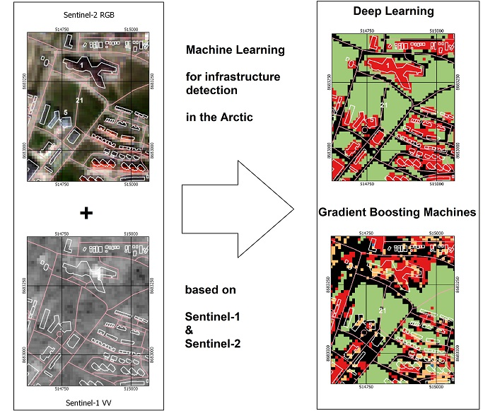
Towards Circumpolar Mapping of Arctic Settlements and Infrastructure Based on Sentinel-1 and Sentinel-2

Abstract

Infrastructure expands rapidly in the Arctic due to industrial development. At the same time, climate change impacts are pronounced in the Arctic. Ground temperatures are, for example, increasing as well as coastal erosion. A consistent account of the current human footprint is needed in order to evaluate the impact on the environments as well as risk for infrastructure. Identification of roads and settlements with satellite data is challenging due to the size of single features and low density of clusters. Spatial resolution and spectral characteristics of satellite data are the main issues regarding their separation. The Copernicus Sentinel-1 and -2 missions recently provided good spatial coverage and at the same time comparably high pixel spacing starting with 10 m for modes available across the entire Arctic. The purpose of this study was to assess the capabilities of both, Sentinel-1 C-band Synthetic Aperture Radar (SAR) and the Sentinel-2 multispectral information for Arctic focused mapping. Settings differ across the Arctic (historic settlements versus industrial, locations on bedrock versus tundra landscapes) and reference data are scarce and inconsistent. The type of features and data scarcity demand specific classification approaches. The machine learning approaches Gradient Boosting Machines (GBM) and deep learning (DL)-based semantic segmentation have been tested. Records for the Alaskan North Slope, Western Greenland, and Svalbard in addition to high-resolution satellite data have been used for validation and calibration. Deep learning is superior to GBM with respect to users accuracy. GBM therefore requires comprehensive postprocessing. SAR provides added value in case of GBM. VV is of benefit for road identification and HH for detection of buildings. Unfortunately, the Sentinel-1 acquisition strategy is varying across the Arctic. The majority is covered in VV+VH only. DL is of benefit for road and building detection but misses large proportions of other human-impacted areas, such as gravel pads which are typical for gas and oil fields. A combination of results from both GBM (Sentinel-1 and -2 combined) and DL (Sentinel-2; Sentinel-1 optional) is therefore suggested for circumpolar mapping.

1. Introduction

The Arctic environment is changing rapidly due to climate change [1], but also due to direct human impacts [2,3]. Infrastructure expansion is driven by exploitation, transport routes, and military history. Arctic infrastructure has expanded in many regions in recent decades following industrial development. We find nowadays a mixture of settlements of indigenous communities and cities resulting from industrial growth. The manifold environmental impacts have been documented extensively with remotely sensed methods. This includes consequences of air pollution for vegetation [4,5,6], oil spills [7], loss of biodiversity [8], and mechanical disturbances [9,10]. Industry and disturbance-related landcover classes were introduced in such context in some cases, but their accuracy was not always assessed (see, e.g., in [6,9]). Virtanen et al. [10] included and assessed a general class “Human infrastructures” (cities, villages, industrial areas, railroad, and main roads) for the Usa Basin, Russia. Infrastructure in the Arctic also modifies ground temperature (see, e.g., in [11]) and is impacted by permafrost thaw [12,13,14]. Specifically coastal settlements are affected by rapid coastal erosion in ice rich permafrost regions [15]. Several studies therefore tried to assess the impact of climate change on Arctic infrastructure including those in Hjort et al. [13] and Suter et al. [14]. A major obstacle for these studies is precise geospatial information on location and extent of settlements across the Arctic. A number of global build-up area datasets exist (see, e.g., in [16,17]), but also roads and other features are of relevance. According to Raynolds et al. [3], the infrastructure footprint in Arctic coastal regions includes roads, gravel pads, and mines (excavation sites) as surface features. The largest area coverage (based on analyses of aerial photographs) among these types on the Alaskan North Slope have gravel pads. Studies which investigate the impact of climate change on Arctic infrastructures situated on permafrost (such as Suter et al. [14]) use datasets of roads, railways, buildings, and airport strips. Buildings, airport strips, and ports are usually represented as points. Linear infrastructure includes roads, railroads, and pipelines. Publicly available sources (national data, OpenStreetMap or similar) are merged to obtain a circumpolar coverage. This leads to inconsistencies and also excludes gravel pad features. OpenStreetMap is globally available, but is inconsistent and incomplete across the Arctic. It has been also used as one of the main sources for the analyses in Hjort et al. [13] due to the lack of an alternative data source. Buildings were converted to point features and only roads of a certain importance have been considered to account for inconsistencies regarding minor roads. Furthermore, here, only roads and buildings excluding the surrounding grounds were considered part of the infrastructure. The number of features within a certain area is then considered for risk assessment.

Settlements and infrastructure features are comparably small in the Arctic and require a certain spatial resolution for their identification. Many small settlements exist. Further on, new infrastructure related to oil and gas developments drives so-called linear strip development [18] of settlements. The road network therefore shapes the overall structure in some regions, including part of the Alaskan North Slope and Western Siberia. Global landcover datasets are in general of too low spatial resolution and also lack thematic content to successfully identify such features. Satellite-based landcover mapping in the Arctic usually targets description of the natural environment [19]. The often used 30 m Landsat data provide only limited applicability for settlement and infrastructure detection. Many Arctic settlements are included in the Global Man-made Impervious Surface (GMIS [20]) and the Human Built-up and Settlement Extent (HBASE [16]) which are based on Landsat, but are incomplete and also lack subcategories. Mapping therefore usually involves interpretation of areal photographs and high spatial resolution satellite data (see, e.g., in [2,3]). Manual extraction (vectorization) has been the main method for utilization of remotely sensed data for identification of infrastructure in the Arctic so far. Due to limited availability of such data (very high resolution image availability and vectorization effort), these studies have been always locally confined. Kumpula et al. [2,21] assessed the applicability of different satellite data for industry related mapping on central Yamal, Western Siberia, Russia. Small scale features (<0.09 ha) and local removal of topsoil and vegetation as part of construction projects, proved especially challenging to identify. ASTER and SPOT with 15 m and 20 m resolution, respectively, were shown superior to Landsat. Compared to SPOT, ASTER could also be used for manual identification of pipelines and drilling towers as well as single off-road vehicle tracks. The main challenges concern spectral characteristics. Similar spectral signatures between sandy areas and human made surfaces including gravel roads and pads are observed.

Synthetic aperture radar (SAR) can be also used to identify aspects of the human footprint due to double-bounce, the predominant backscattering mechanism for buildings, which leads to higher backscatter amplitude than in the surroundings. For example, Blasco et al. [22] estimate that double-bounce contributes to 24% of backscatter for urban pixels in case of C-band (based on fully polarimetric data). Related workflows focus in general on built-up areas only (see, e.g., in [17,23]) due to the good separability from other landcover types. Moreover, here ambiguities are manifold. Many other surfaces are misclassified as built-up (e.g., high backscatter also occurs over block fields). An external data source is required in order to pre-select areas with settlements for manual postprocessing. The insufficiency of such records in turn reduces the potential for improving settlement records. For example, the Global Urban Footprint (GUF) dataset based on TerraSAR-X [17] leaves out many smaller settlements across the Arctic. Iannelli and Gamba [24] suggest a combination with derivatives from digital elevation models to at least treat ambiguities in mountain areas. In addition to the backscatter amplitude, texture can be utilized [25] to improve built-up area detection. Utilizing repeated acquisitions, interferometric SAR coherence can be combined with backscatter intensity to derive built-up areas (the authors of [23,26] tested for semi-arid and arid regions). Results by Corbane et al. [26] for a town in the Netherlands suggest that the use of coherence (VV) increases the error of omission but performance increases with decreasing built-up density. The association of built-up areas or urban footprint with certain landcover classes varies across studies. Talukdar et al. [27] include, for example, roads in built-up areas with focus on multispectral data only. Stromann et al. [28] treat roads as a separate class and distinguish between low- and high-density built-up areas. However, in general, only the term “urban area” is used and binary outputs (urban versus none urban) are generated.

A further challenge in this context is the variation in acquisition strategies of SAR missions across the Arctic. Sentinel-1, for example, acquires in different polarizations with varying coverage. Developments targeting global coverage focus on VV+VH (see, e.g., in [17,23]) as this is the dominant setting for land areas globally. In the Arctic, acquisitions are, however, partially made in HH+HV due to requirements by sea ice and glaciology-related applications. The viewing direction of the sensor and orientation of building walls also plays a role in detectability [29,30]. Depending on the properties of the feature, objects are spatially offset in the resulting images. Size-related offsets in SAR vary in direction from offsets in optical images [31].

The Sentinel satellites of the recently initiated European Copernicus Mission are expected to provide an improvement for this type of application. Optical as well as radar data are acquired in resolutions starting from 10 m. It is estimated that Sentinel-2 can identify roads starting from 3 m width in agricultural environments [32]. This opens the way for the identification of buildings and roads of dimensions as can be found in the Arctic. The task, however, is data intensive, and cannot be accomplished manually (as in previous studies [2,3]) across the entire Arctic. Threshold approaches for SAR and applications of indices (Normalized Difference Built-up Index [33] or the Index-based Built-up Index [34]) in case of multispectral data alone are often of limited applicability [24]. Machine learning techniques have been shown applicable in other environments than the Arctic for settlement detection (see, e.g., in [35,36,37,38,39]). Specifically, deep learning is expected to allow identification of human footprint-related features and to deal with ambiguities. A range of remote sensing studies, including in urban environments, exist for these approaches [40,41].

A challenge for semiautomatic techniques is the need for extensive training data. Settlements in Arctic environments are usually small and only scarce reference data exist (limited to areas of manual HR (high resolution) image interpretation). This requires sparsity-aware algorithms. Gradient boosting machine (GBM) learning, as suggested by Chen and Guestrin [42], is expected to be applicable for sparse data. It has been shown to outperform support vector machines (SVM) or random forest for VHR (very high resolution) data in urban environments [37]. This may also apply to 10 m resolution, which resolves many relevant artificial objects better than, e.g., Landsat [2,21]. Stromann et al. [28] tested Sentinel-1 and -2 with SVM for urban environments with good results, but did not compare it to other approaches.

A further option is deep learning, which is a special type of machine learning that can solve more complex problems. Deep learning-based semantic segmentation generally uses convolutional neural networks (CNNs). This method is usually applied in the context of using VHR optical and SAR data. Deep learning has been shown to reduce additional (manual) mapping efforts for delineating the urban footprint from Tandem-X/TerraSAR-X data [39]. It has been applied using VHR optical data for mapping (informal) urban villages in China [36], and informal settlements in Africa [38,43,44]. Wurm et al. [45] combine Sentinel-2 and TerraSAR-X data for informal settlement detection. Deep learning has so far not been tested for human footprint identification in tundra environments. Here, we cannot utilize VHR data yet for the entire Arctic (access limitations, data amount), but Sentinel-2 is expected to provide the required detail in this context (identification of roads and small features as typical for tundra settlements). Road monitoring applications based on SAR data are usually focusing on subsidence monitoring, but deep learning, specifically the UNet neural network architecture [46], has been shown to be of value for road extraction from Sentinel-1 backscatter amplitude [47]. Furthermore, the results of Zhao et al. [41] for cities in China demonstrate the superior performance of deep learning for separation of urban targets from Sentinel-1.

The added value of Sentinel-2 for impervious surfaces in urban environments has been, e.g., demonstrated by Lefebvre et al. [48]. Pesaresi et al. [35] also used Symbolic Machine Learning (SML) for detailed urban land cover mapping in central Europe and suggest that Sentinel-1 can complement Sentinel-2 and specifically aid the treatment of ambiguities in Sentinel-2 reflectance. Zhou et al. [49] suggested fusion of Sentinel-1 and multispectral (Landsat) as well as Hyperion (better spectral resolution than Landsat but same spatial resolution). They point out that texture features in SAR are an asset in this context. Iannelli and Gamba [24] investigated the fusion of Sentinel-1 and Sentinel-2 for urban mapping (urban versus non-urban for larger cities). A two step approach is suggested. First, a mask is prepared with Sentinel-2 (combination of several approaches, including random forest), which then serves as input for a threshold-based classification of Sentinel-1 to treat the ambiguities in C-band to some extent. Results match largely the extent of build-up in the GUF dataset. A joint use of Sentinel-1 and Sentinel-2 within a SVM approach is also suggested by Stromann et al. [28] for specific features of large cities (demonstrated for Stockholm and Beijing). High-density and low-density built-up areas have been considered in addition to road features. High-density built-up areas show high confusion with roads and bedrock, whereas low-density is confused with green spaces. In general, only built-up areas and/or larger cities are considered. For Arctic studies, however, information is required for the distribution of not only buildings of smaller settlements with low density, but also roads and other features related to infrastructure.

The objective of this study is to evaluate the capabilities of Sentinel-1 and Sentinel-2 for circumpolar mapping of infrastructure beyond of what is typically represented in global datasets. Target classes include further human-impacted areas (such as gravel pads) in addition to buildings and roads. Two machine learning approaches applicable for data scars settings (gradient boosting machines and deep learning-based semantic segmentation) are assessed and eventually recommendations are formulated.

2. Study Areas and Data

2.1. Satellite Data

The Sentinel-1 and -2 missions are part of ESA’s Copernicus program. Whereas Sentinel-1 carries synthetic aperture radar systems, Sentinel-2 provides multispectral data.

The Sentinel-1 mission consists currently of two satellites with a near-polar, sun-synchronous orbit, 180 degrees apart from each other. The two earth observation satellites Sentinel-1A (launched in April 2014) and Sentinel-1B (launched in April 2016) have an identical C-band SAR sensor onboard [50]. The Interferometric Wide Swath (IW) mode combines a swath width of 250 km with a relatively good ground resolution of 5 × 20 m. A pixel spacing of 10 × 10 m is commonly used for nominal resolution of derived products. This is also the case for Ground Range Detected (GRD) products as distributed by Copernicus. Information can be captured in dual polarization (HH+HV or VV+VH; H—horizontal, V—vertical). Mostly VV+VH is available for the Arctic land area for this mode and resolution. Greenland and several high Arctic islands are covered in HH+HV mode due to requirements of glacial monitoring. The availability of HH and HV, at the same time, varies also over time in this region. More data are acquired in HH only. This results in limitations for certain applications, e.g., regarding mapping of vegetation [51]. Both polarization combinations (HH+HV and VV+VH) are only available for Svalbard, where they are acquired from different orbits (ascending versus descending), resulting in opposing looking directions (Figure 1). GRD products were used for this study. GRD products are detected, multi-looked, and projected to ground range using an Earth ellipsoid model [52]. As temporal variations of backscatter can occur with changes in liquid water content, only winter data (December and/or January; frozen soil conditions) are used for cross-Arctic consistency and comparability (see

Table 1. Validation data and corresponding Sentinel-1 (S-1) and Sentinel-2 (S-2) acquisitions. Reference objects represent areas without any human impact. Dates for Sentinel-2 are provided in Table 2.

Validation Site	Prudhoe Bay	Longyearbyen	Western Greenland
Data source	Raynolds et al. (2014) [3]	Lu et al. (2018) [54]	Ingeman-Nielsen & Vakulenko (2018) [60]
Coverage	3 × 20 km2, 40% non-impacted	31 objects (0.13 km2), 1 reference area (0.42 km2)	253 objects for 7 communities (0.35 km2), 7 reference areas (13.2 km2); (subset for HH+HV coverage area)
Types	Roads and other disturbed areas (especially gravel pads)	Roads (6) and buildings (25)	Roads (27), buildings (199), and other human impact (27)
S-2 granule(s)	05WPU	33XWG	21WXS
			21WXU
			22WDB
			22WDC
			22WDD
			22WDV
			22WEB
			22WEC
			22WEV
S-1 polarization	VV+VH	VV+VH and HH+HV	HH+HV
S-1 dates	06.01.2018	05.01.2019 and 07.01.2019	06.01.2019
S-1 orbit	ascending	descending and ascending	ascending

). The use of such data also allows for simplified normalization with respect to the incidence angle influence on backscatter intensity when deriving the backscatter coefficient ${\sigma }^0$, which is commonly used [53].

The Sentinel-2 constellation has also two twin satellites—Sentinel-2A and -2B—in a sun-synchronous orbit, 180${}^{\circ }$ apart from each other. Sentinel-2A was launched in June 2015 and Sentinel-2B in March 2017. The optical sensor samples 13 spectral bands. The spatial resolution depends on the used band: four bands have a spatial resolution of 10 m, six bands of 20 m, and three bands of 60 m [55]. Bands 2 (blue, 10 m resolution) 3 (green, 10 m), 4 (red, 10 m), 8 (near infrared, 10 m), 11 (SWIR, 20 m), 12 (SWIR, 20 m), 5 (vegetation red edge, 20 m), 6 (vegetation red edge, 20 m), 7 (vegetation red edge, 20 m), and 8A (narrow near infrared, 20 m) have been used for the classifications. Acquisitions from July to early August (snow-free season) have been considered (see, e.g., the selected scenes of the validation granules in

Table 2. Dates of Sentinel-2 acquisitions used for areas with independent validation (see also Table 1).

Sentinel-2 Granule ID	Acquisition Dates
33XWG	01.07.2016, 31.07.2017, 21.07.2018
05WPU	03.08.2016, 10.07.2017, 24.07.2017
21WXS	13.08.2016, 03.08.2017, 13.08.2017
21WXU	08.08.2017, 26.08.2017, 06.08.2017
22WDB	13.08.2016, 08.08.2017, 15.08.2017
22WDC	03.08.2016, 06.08.2016, 06.08.2017
22WDD	27.07.2016, 26.08.2016, 02.07.2018
22WDV	21.07.2017, 28.07.2017, 31.07.2017
22WEB	11.07.2016, 30.08.2016, 15.08.2017
22WEC	13.08.2016, 29.07.2017, 19.07.2018
22WEV	12.08.2017, 28.07.2017, 13.07.2018

).

2.2. Study Areas and Calibration and Validation Data

Consistent information on human impact is required across the entire Arctic and is of special concern in settings with presence of permafrost [12,13,14]. The areas of interest have therefore been selected with respect to permafrost extent (source: [56,57]). All calibration and validation sites are located in sporadic to continuous permafrost (Figure 3).

High spatial resolution datasets are required in order to calibrate and validate the landcover classifications. This needs to reflect requirements by the algorithms, satellite data availability, environmental settings (potential reflectance ambiguities), and target categories. The relevant categories (roads, buildings, and gravel pads) need to be included. Ideal sources are vector datasets which are based on aerial photographs and/or very high spatial resolution satellite data. Published datasets are, however, scarce. The records in [3,58] include three sites (each 20 km²) at the Prudhoe Bay oil extraction site for which human impact on the environment has been mapped. This area is characterized by herbaceous shrub tundra. This region was the first developed oilfield in the Arctic, and is the largest in the United States. The built-up layer of the Global Human Settlement (GHS) dataset [59] includes approximately 30 250 × 250 m pixels with up to 20% coverage in the proximity of Prudhoe Bay, which indicates presence of human impact but provides no information on actual objects. The records in [3] consider changes after 1968 up until 2011. Openly available datasets in other environmental settings are lacking. This is a challenge for settlements which are different from the Prudhoe Bay environmental setting, specifically those which are largely build on bedrock. Misclassifications are expected in such areas due to reflectance ambiguities which need to be assessed. A dataset has therefore been specifically assembled for the Greenland West coast (eight settlements) and Svalbard (Longyearbyen). Longyearbyen is neither represented in the GUF [17] nor in the GHS. Four of the Greenland sites are covered by the GHS and six out of the eight in the GUF (12 m, 2012 version). Cadastral information has been selected from national sources, checked as part of an in situ campaign in 2018, and annotated. Surface and roof types have been mapped (Figure 2) as well as functions (public, industrial, and residential) of buildings [54,60]. Datasets are complemented with a reference area in the proximity for each covered settlement. This reference area represents a typical environmental setting and does not include any infrastructure or human impact. The Prudhoe Bay, Greenland and Svalbard datasets are used for independent (of data record types used for calibration) validation in our study. Dataset characteristics of the validation records and used acquisitions over these regions are provided in Table 1 and Table 2.

Algorithms such as deep learning require a large amount of training data. OpenStreetMap data are therefore commonly used as input for deep learning in remote locations (see, e.g., in [39]). Such data can provide useful information in densely populated areas where completeness and accuracy can be expected to be relatively high. The majority of settlements are, however, not fully represented in the Arctic, which delimits the choice for calibration areas. Approximately 12,000 building and 3200 road objects have been used. They represent the complete set of available features within the selected Sentinel-2 granules. Streets and building information is available in vector format via OSM Geofabrik (Geofabrik GmbH, Karlsruhe, Germany, http://www.geofabrik.de/), but other human-impacted areas are not precisely included. An alternative source is required. The Google online hybrid map includes very high resolution images for some Arctic settlements. It has been therefore used to identify human-impacted areas across several Sentinel-2 granules for the deep learning (Figure 3). It has been further used to assemble a training dataset dedicated for the pixel-based machine learning approach. Specific emphasis was on selection of sufficiently large areas (with respect to the 10 m spatial resolution) and homogeneous properties in this case.

3. Methods

An automated workflow for downloading, preprocessing, and classifying Sentinel-1 and Sentinel-2 data has been set up with the mapping of the coastal infrastructure with circum-Arctic extent as a final goal. We further classified with two different methods, one being a pixel-based classification using a Gradient Boosting Machine [42] and the other being a windowed semantic segmentation approach using the deep learning framework keras [61] with the Tensorflow backend, referred to as GBM and DL, respectively, in the following.

3.1. Preprocessing of Satellite Data

Data from a total of 50 Sentinel-2 granules have been considered for this study. Sentinel-2 data are available as granules (100 × 100 km tiles) in UTM projection and largely at Level 2A (orthorectified, top of atmosphere). As the data are available for top-of-atmosphere reflectance only, atmospheric correction was required in addition to cloud masking. Sentinel-2 provides a spatial resolution of 10 m for some bands but not for all. As shown by Kumpula et al. [2], scale is crucial for Arctic infrastructure and impact mapping. Enhancement of spatial resolution of the coarser band therefore needs to be considered to exploit the multispectral capabilities offered by Sentinel-2.

In order to account for anomalies due to undetected clouds in Sentinel-2, three acquisitions have been combined. They represent the same year where possible, but in most cases several years were utilized (see, e.g., dates for validation sites in Table 1). This strategy does, however, require atmospheric correction in order to account for related differences between the dates. We therefore applied atmospheric correction using sen2cor on the Sentinel-2 data, which also generates a cloud mask during the process. We further performed super-resolution based on the tool Dsen2 [62], which uses a convolutional neural network. Lanaras et al. [62] showed that their approach clearly outperforms simpler upsampling methods and better preserves spectral characteristics. The original model was trained on Level-1 data, which have not been atmospherically corrected, and global sampling. We therefore retrained and tested their model on Level-2 data (output of sen2cor) using the same published training and testing routines (https://github.com/lanha/DSen2) for selected granules from our study sites (acquired only in July and August). The code was only modified to read in the Level-2 data. We used nine Sentinel-2 scenes for training and three scenes (subset of classification calibration granules, see Figure 3) for testing of our model, which amounts to one-fifth of the dataset sizes used by Lanaras et al. [62] for their global model. The Root Mean Square Error (RMSE) between the original 20 meter resolution data and the result of super-resolution performed on synthetically downsampled 20 meter resolution data is the primary suggested evaluation metric [62]. It has been therefore applied for evaluation. After the super-resolution step, clouds were masked using the cloud mask output from sen2cor.

For preprocessing of Sentinel-1, we applied border noise removal, based on the bidirectional all-samples method of Ali et al. [63], calibration, thermal noise removal, and orthorectification using the digital elevation model (DEM) GETASSE30 (Global Earth Topography And Sea Surface Elevation at 30 arc second resolution; as shown applicable in [53]). These steps were carried out with the Sentinel Application Platform (SNAP) toolbox provided by the European Space Agency and ${\sigma }^0$ was derived. The backscatter–incidence angle relationship varies by landcover type and needs to be determined for each location to allow normalization and subsequent combination and comparison of scenes over space and time. This is specifically of concern when large areas need to be covered. Otherwise, typical striping patterns in orbit direction (across near to far range of the radar scene) occur (e.g., as seen in Figures 9 and 10 of Mahdianpari et al. [64], ). Widhalm et al. [53] suggest a simplified method which is applicable to frozen tundra environments. A linear dependency is assumed with validity for an incidence angle range of approximately 20${}^{\circ }$ to 45${}^{\circ }$. A challenge for normalization of Sentinel-1 data in our case is posed by the variable availability of polarizations (HH and HV versus VV and VH). So far, normalization parameters have been published only for HH and VV [51,53]. Models still need to be calibrated for HV and VH. Existing studies used a landcover map based on Landsat for the Usa Basin which is located to the west of the Northern Urals, Russia (Usa Basin, Russia, Virtanen and Ek [65]; see also Bartsch et al. [19], Widhalm et al. [53], and Bartsch et al. [51]). Data from multiple orbits, representing a range of incidence angles for each location, need to be used. Representative scenes over the Usa Basin have been therefore preprocessed in addition, and a function was fit to each landcover-specific sample to describe the relationship of the local incidence angle with ${\sigma }^0$ for VH (IW mode) and HV (enhanced wide swath mode). The relationship between the slope values k for all the different landcover classes and ${\sigma }^0$ at 30${}^{\circ }$ was eventually derived in order to obtain the normalization functions.

After normalization of the Sentinel-1 data, a mosaic was created for each sub-region, and reprojected and subset to match the Sentinel-2 granules extent.

3.2. Calibration and Model Assessment Data Preparation

The different requirements of the algorithms as well as the inconsistencies in the input dataset (satellite data as well as calibration data) need to be considered. Two sets of training data have been therefore generated: one set for each of the tested algorithms. They consist of separate datasets for each of the polarization mode combinations (VV+VH and/or HH+HV as available), due to the spatial variability in polarization of the Sentinel-1 coverage (Figure 4). For assessment of model efficiency (referred to as internal assessment in the following; usage of data consistent with the calibration data), the datasets have been split into two parts. The proportion used for internal assessment was 40% in case of GBM and 20% for DL. The separation was made randomly. Twenty percent is commonly used for DL [66]. A comparably large amount of training data is needed in this case. This is less critical for GBM. Therefore, twice the amount was used for calibration. In order to demonstrate the need for targeted calibration data for each approach, the GBM algorithm has been tested also using the dataset created for DL. A proportion of 40% has been selected for internal assessment in this case to ensure comparability.

The calibration dataset for the deep learning based on OpenStreetMap initially does only include buildings and roads in vector format. In order to represent other human-impacted surfaces, additional information must be collected manually for this class for selected settlements with high spatial resolution coverage in Google Hybrid Maps. The training information also needs to be spatially complete for a certain area (window; here 512 × 512 pixel) in the case of deep learning. The vectors (polygons and lines) have been rasterized matching the 10 m spatial resolution of the Sentinel data. Pixels along the line render path, in case of lines and pixels that have their center inside polygons in case of polygons, were considered during rasterization. The total DL training area covered approximately 7000 square kilometers and has been applied for VV+VH and/or Sentinel-2 use. The area which can be potentially covered with sufficient quality training data for HH+HV extent (Greenland and Svalbard) is too small for DL calibration. HH+HV application with DL was therefore excluded from the analyses.

As an alternative to OpenStreetMap, which does not reflect limitations of satellite records (especially spatial resolution), an additional calibration dataset has been prepared based on visual interpretation of high resolution datasets available in Google Hybrid Maps, as well as the Sentinel-1 and 2 data available over the selected sites in case of GBM. In total, 463 polygons have been defined in the proximity of Varandai, in the Northern Urals, and on the Yamal peninsula (all in Russia, see Figure 3) for the Gradient Boost Machine algorithm for classifications with VV+VH: 156 polygons for the road class, 141 polygons for the building class, and 166 polygons for other human-impacted areas (bright objects). Similarly, for classifications with the HH and HV channel of Sentinel-1, 65 polygons for the road class, 79 polygons for the building class, and 32 polygons for other human-impacted areas (bright objects) have been defined within the HH+HV covered area, in the vicinity of Longyearbyen & Barentsburg (Svalbard, Norway), as well as Ilulissat and Aasiaat (Greenland). The polygons represent target objects which are relatively large (extent over several pixels) and are homogeneous. Samples have been also collected for water bodies and shrub to herbaceous tundra areas in order to spectrally separate these areas in the pixel-wise GBM classification. This type of dataset is referred to as the Region of Interest (ROI) dataset in the following.

3.3. Gradient Boosting Machine Learning

The GBM algorithm has been calibrated with the ROI dataset (specifically created for GBM, see previous section) and the rasterized tiles (windows created for DL) in order to evaluate the need for dedicated calibration records. In both cases, 60% has been used for calibration and 40% for internal assessment. The separation has been based on a stratified random selection. Different versions have been computed to test the effect of including Sentinel-1 data with varying polarizations and compare the results to each other. We used a gradient boosting tree classifier from the xgboost library [42], which has the advantage that it provides support for the graphics processing unit (GPU), leading to significant speed-up during training and prediction. Gradient boosting improves the quality of fit. Each regression tree contains a continuous score on each of the leafs. During training, we used 10-fold cross-validation (training set split into ten equally sized parts, run ten times with each part acting as validation set once and the remaining nine parts as training set) and the macro-averaged F1-score (arithmetic mean over class-wise F1-scores, also known as Dice similarity coefficient) for hyperparameter selection. Specifically, we tested combinations for the number of trees, maximum tree depth, and learning rate of the GBM classifier, but these parameters had to be restricted in favor of prediction time. The model with the combination that obtained the highest macro-averaged F1-score during cross-validation was automatically selected for the final training and prediction steps. The selected parameters are a learning rate of 0.1 and maximum tree depth of 3 for all data combinations (ten different models were trained with different polarization combinations and input data). The selected number of trees varies across models and is either 500 or 1000. The trained models were saved as PKL files (Python Pickle File—for serialization of objects at runtime) and used to classify entire granules in the following.

Target classes additionally include water and tundra for better separability (see

Table 3. Target class descriptions and use for Gradient Boost Machines (GBM) and Deep Learning (DL), respectively.

Target Class	Description	GBM	DL
Buildings	houses, industrial buildings including tanks	x	x
Roads	gravel as well as asphalt roads (no tundra tracks)	x	x
Other human impacted area	gravel pads, air strips, moorings	x	x
Tundra	All natural landcover, excluding water	x
Water	Open water	x

). They represent the main landcover classes surrounding Arctic settlements.

3.4. Machine Learning Based on Neural Networks—Deep Learning

We split the training granules into tiles of 512 × 512 pixels with an overlap of 256 pixels and selected a total of 459 of these 512 × 512-tiles for training. The labeled masks required for training were obtained through a rasterized version of the reference data likewise. The dataset was further split into training (80%) and validation (20%) sets used during the training process. Due to the nature of the data (raster), a random split has been applied for the separation of the two sample sets. The selection of the appropriate ratio of tiles with and without infrastructure reference was found to be critical for model convergence and was obtained in a trial-and-error fashion. The Keras library [61] was used for the implementation of the training and classification routines, which were also run on GPU for computational efficiency. We used a UNet neural network architecture [46], which is especially useful for small datasets, as it is clearly the case here. Here, small refers to the number of images commonly used for training CNNs (often tens of thousands in case of semantic segmentation [67]). In contrast to pixel-based classification, deep learning-based semantic segmentation can capture context information [46]. That is why we expect it to be useful even for a small number of training images. We used data augmentation in the form of horizontal and vertical flips of the images (see, e.g., in [68,69,70]). We used a custom loss function and metric for monitoring progress during training. A commonly used metric for semantic segmentation with deep learning is also the F1-score, which is here often referred to as the dice similarity coefficient. The proposed metric is the global average of all the dice similarity coefficients calculated for each class separately. Therefore, it is essentially calculated the same way as the macro-averaged F1-score used with the GBM classifier, but it uses probabilities instead of the hard class values. The loss function used for training is the complement of the averaged dice coefficient (one minus the averaged dice coefficient). The classification of entire Sentinel-2 granules was conversely performed using a sliding window of 512 × 512 pixels, again with an overlap of 256 pixels.

Target classes in the case of DL are confined to the artificial object types (see Table 3). Other surrounding landcover types do not need to be considered due to the nature of the deep learning algorithm.

3.5. Validation Strategy

Model efficiency assessment based on the separated proportion of the two algorithm-specific datasets has been carried out in a first step (see previous sections on the classification algorithms). External datasets have been used in a second step for independent assessment. The external datasets are not consistent with respect to all tested regions (type of settlement and environment as well as coverage by specific polarizations). However, they have been nevertheless utilized for an independent assessment as they are not algorithm specific selections (see Section 2.2). Confusion matrices have been extracted for external validation, covering users and producers accuracy in percent.

4. Results

4.1. Normalization Parameters for HV and VH and Performance of the Adapted Super-Resolution Scheme

A linear relationship between the slope (characterizing the local incidence angle and backscatter relationship) and frozen condition backscatter is apparent for the tested landcover types with an $R^2$ of 0.91 for HV and 0.70 for VH (Figure 5). HV- and VH-polarized backscatter at C-band is in general lower than for equal polarization, but the relationship of HV and VH backscatter is almost identical among each other (Figure 5) and similar (just off-set) to HH [53] and VV [51].

The RMSE of our model for the super-resolution scheme (28.9) is lower than the one reported for the original model (34.5 [62]). Values are given in digital numbers (DN) of the Sentinel-2 data, which is reflectance multiplied by 10,000.

4.2. Model Efficiency Assessment

The best results are obtained for combination of Sentinel-1 with Sentinel-2 using gradient boost machine learning (see

Table 4. Model efficiency assessment results (F1-score) for the Gradient Boost Machine (GBM) and the Deep Learning (DL) algorithm. Separation by polarization combination of Sentinel-1 data (V-vertical, H-horizontal). The column “Tundra/other” reflects the tundra class in case of GBM-specific training data both waterbodies and tundra in case of use of DL-specific samples.

Type	Method	Input	Training Score	Testing Score	Road	Tundra/ Other	Building	Other Human Impact	Water
VV+VH	GBM	VV	1.00	0.97	0.88	1.0	0.97	0.99	1.0
	GBM	VH	1.00	0.96	0.87	1.0	0.96	0.99	1.0
	GBM	VV+VH	1.00	0.97	0.9	1.0	0.97	0.99	1.0
	GBM	VV based on DL samples	0.61	0.60	0.47	0.89	0.42	0.63	n.a.
	GBM	Sentinel-2 only	0.94	0.94	0.84	1.0	0.88	0.97	1.0
	GBM	Sentinel-2 only based on DL samples	0.60	0.59	0.43	0.89	0.39	0.64	n.a.
	DL	Sentinel-2 only	0.83	-	-	-	-	-
	DL	VV	0.61	-	-	-	-	-
	DL	VH	0.61	-	-	-	-	-
	DL	VV+VH	0.81	-	-	-	-	-
HH+HV	GBM	HH	1.00	0.92	0.88	1.0	0.76	0.97	1.0
	GBM	HV	1.00	0.90	0.86	1.0	0.69	0.98	1.0
	GBM	HH+HV	1.00	0.94	0.91	1.0	0.81	0.98	1.0
	GBM	Sentinel-2 only	0.99	0.88	0.84	1.0	0.6	0.97	1.0

). A combination does not lead to a higher score in the case of DL. The highest F1-score is achieved with the use of Sentinel-2 only. A similar level of accuracy is, however, reached when both available polarization bands (VV+VH) are used in combination with Sentinel-2.

The available schemes provide class specific scores for GBM only. The highest scores are reached for “other human impact” in all cases. The GBM results for the other classes differ between VV+VH and HH+HV combinations. The accuracy of road identification is lower compared to buildings in the case of VV and/or VH. The opposite is the case for HH and/or HV usage. The actual score for roads is, however, similar for the polarization combinations. This suggests best performance for VV and/or VH combinations. The usage of samples dedicated for application with gradient boost machine learning clearly provides better results for this method than usage of the OpenSteetMap-based sample dataset created for DL.

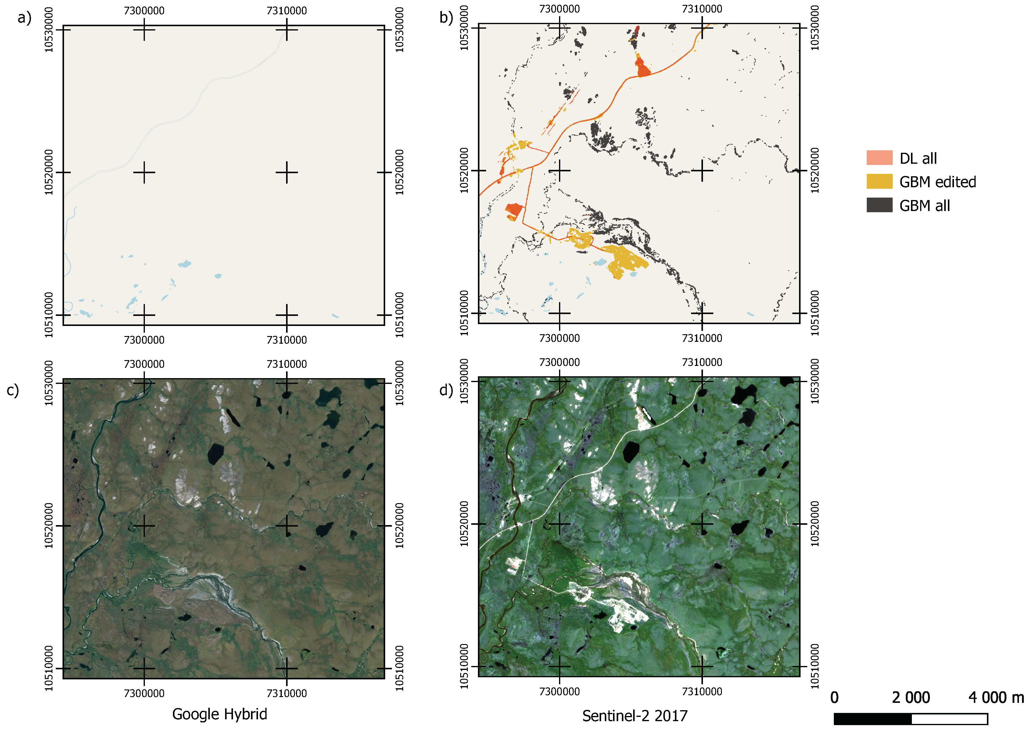
4.3. Assessment with External Data

The main sites for testing the performance of the algorithm are Prudhoe Bay, Western Greenland, and Svalbard. The Prudhoe Bay data allow assessment of users and producers accuracy as it also provides spatially continuous information on other classes than human impact.

The results for Longyearbyen confirm the performance difference between VV+VH and HH+HV (Figure 6) as already shown with the model efficiency assessment. Buildings are better detected with HH+HV and roads with VV+VH. The ability of the deep learning approach to separate human-made objects from the surroundings can be clearly shown for this area. Whereas DL achieves 100% accuracy, GBM shows errors of 40% and higher. The combination of Sentinel-1 with Sentinel-2 does not lead to better results for all categories compared to usage of Sentinel-2 only in case of DL based on the full record in Lu et al. [54]. An example which shows the University of Svalbard (UNIS) building demonstrates, however, the potential added value of Sentinel-1 VV+VH (Figure 7, ID #1). The full extent is only captured with VV+VH inclusion. The consideration of at least VV or HH, respectively, is of advantage in case of GBM (Figure 6). This is also confirmed by the results for Greenland (Figure 8).

The users accuracy derived for the Prudhoe Bay area shows similar performance for GBM and DL in the case of roads (Figure 9). GBM shows better results for buildings than DL. In general, many objects are not detected by both algorithms. This is especially the case for roads (~60% not included), but also for other human-impacted areas (~40%). Only fragments of roads are identified by both algorithms (see Figure 10c,d). However, the results indicate that the spatial resolution is sufficient to identify the presence of roads, although not their complete extent. DL results do not include all human impacted area. Often only a proportion of gravel pad is detected (Figure 10d). They are better represented in the GBM results but many other natural surfaces which are bare of vegetation are included, e.g., river banks.

4.4. Surface Types and Building Properties

Roof material and shape play a role in the detectability of buildings. As these can be associated with certain uses, this also causes differences between residential, industrial, and public buildings. The capabilities of VV and HH polarization are distinct according to the results for Longyearbyen, where both are available (Figure 11). The inclusion of HH in the GBM classification leads to better results than with VV in all cases. Agreement ranges between 60 and 90% for all material types except for wood roofs. Percentages are highest for sloped roofs. This can be confirmed with the comparisons for Greenland (Figure 12), although the agreement is much lower than at Longyearbyen for other types. An agreement of more than 60% can be reached with VV only in case of metal roofs.

The usage of Sentinel-1 for the deep learning approach does not lead to differences in detectability regarding building and road types (Figure 11). Deep learning results are similar to GMB based on inclusion of Sentinel-1 with HH polarization. This can be confirmed with data from the Greenland sites (see Figure 12). DL clearly outperforms GBM only in case of buildings with roofs from wood.

Building size clearly plays a role for identification (Figure 13). Buildings smaller than 1000 m² have been in several cases not detected by both classification types at Longyearbyen. Partial identification is common for the Gradient Boosting Machine results, both in case of VV&VH and HH&HV. Moreover, smaller objects can be identified fully with the deep learning approach and partial identification is less common (only 20%; further 20% undetected and 60% completely covered).

The assessment results for road types differ between Longyearbyen and the Greenland settlements. Deep learning seems to be more appropriate in the case of Longyearbyen. Gradient Boosting Machines appear to be superior for the Greenland sites for both cases gravel and asphalt roads. As expected, asphalt roads can be better separated than gravel roads.

5. Discussion

5.1. Sensor-Specific and Scene Selection Issues

The combination of several Sentinel-2 acquisitions to deal with undetected clouds has been shown applicable in Arctic regions before [51]. A challenge is the short snow-free season and subsequently phenological stages. We have chosen July to August as months for scene selection. Snow patches could still occur in some years at northern sites in July. A check for snow presence (e.g., based on the Normalized Difference Snow Index) might be necessary for circumpolar application. The usage of late season acquisitions (September) may lead to different results in separability from the surrounding tundra.

In most cases, acquisitions from several years (up to three) needed to be combined (Table 2). Changes in landcover (construction of new roads, etc.) during that period may therefore not be fully represented. The first acquisition is therefore the most applicable time stamp for the classification. The full time span should, however, be included in the meta data of any derived product. An alternative would be to use only one cloud-free image, but detailed visual inspection would be necessary for each granule and the assumption made that undetected clouds can be manually identified. Such a strategy is expected to nevertheless lead to spatial inconsistencies as dates and years of suitable scenes vary across the Arctic.

Previous studies which target larger area coverage have focused on VV+VH usage in case of Sentinel-1 as this is the commonly available acquisition mode [23,71,72]. Our results indicate that Sentinel-1 VV+VH and HH+HV provide complementary information with respect to the infrastructure types of interest. A combination would be theoretically possible for Longyearbyen, where both data types are available. The polarization combinations are, however, acquired from different orbits—ascending and descending. This leads to differences in acquisition geometry and spatial offset of associated backscatter in the case of buildings. Higher backscatter related to a certain building can be spatially offset by several pixels (Figure 1). Quadpol acquisitions would therefore be of advantage. Such data are potentially available in C-band for the Arctic from Radarsat-2, but not spatially consistent and with access restrictions.

The spatial offsets in case of buildings in SAR data also subsequently pose a major issue when combined with multispectral data. The detectability of objects with SAR strongly depends on shape and exposition with respect to the sensor (see, e.g., in [29,30]). This effect may explain specifically the partially lower performance of the combined versus the Sentinel-2 only version in case of the deep learning algorithm (compare, e.g., Figure 6). The misalignment is expected to reduce the separability of objects. This difference is not apparent in the GBM accuracy values, which may partially result from the fact that the training data has been defined taking sensor-specific properties into account (spatial resolution and heterogeneity). The impact of the misalignment effect could not be tested for combination of HH+HV and Sentinel-2 in case of the deep learning algorithm. The limitation of Sentinel-1 availability for HH+HV to Greenland and Svalbard reduces the extent of the training dataset considerably. The usage of the full coverage of cadastral information for training instead of OpenStreetMap may allow for an extension to HH+HV usage.

The direct HH+HV and VV+VH comparison was only possible for Longyearbyen, Svalbard. This settlement is located in an area with rather sparse vegetation. The performance differences may differ for tundra regions with higher vegetation coverage, specifically misclassifications are expected to be lower.

5.2. Suitability of Algorithms

The simplified normalization approach introduced in [53] for HH can be shown applicable for all available polarization combinations of Sentinel-1 (Figure 5). This enables operational preprocessing. The good performance (better RMSE than reported before) of the adapted super-resolution scheme could be explained with the regional focus. Lanaras et al. [62] explicitly note that it is likely that even better results than theirs could be achieved, if a user focusing on a specific task and geographic region retrains their proposed network with images from that particular environment.

Both algorithms have been selected due to their known performance in case of scarce data. The training data generation still poses a major challenge for Arctic settlement detection. For example, DL training for HH+HV could not implemented. Too few settlements exist for Greenland and Svalbard (the only regions for which HH+HV acquisitions are available) with good quality data as part of OpenStreetMap data. The definition of calibration areas for GBM requires the availability of very high spatial resolution satellite data in order to identify relatively homogeneous objects. Availability of such data is also limited across the Arctic.

The performance of the algorithms differs between the classes and each shows weaknesses in certain cases. GBM provides better detection of gravel pads (see Figure 10). DL clearly represents roads in their linear shapes, but other human-impacted areas are not fully detected. The error of commission in the GBM results is, however, very high, especially when river banks, beaches, and bedrock surfaces occur. They are often misclassified as buildings and other human-impacted areas. This requires extensive manual postprocessing. DL (Sentinel-2 only)-based detection of single buildings is more complete than with GBM (Figure 13). This can be also seen when compared to OpenStreetMap data in case of Longyearbyen (Figure 7). Both buildings, which are part of the validation dataset (#1 and #5), are composed of a mixture of classes in the GBM results. A combination of results from both algorithms might aid automatization, for example preselection of objects/target regions based on the DL classification based on Sentinel-2 only. A similar two-step approach was suggested in Iannelli and Gamba [24] in the case of urban area detection of larger cities.

As HH+HV is unavailable in IW mode for most of the Arctic, the target class “buildings” should be therefore preferably derived based on the deep learning method. Whereas roads and buildings have specific shapes, other human-impacted areas do not. The advantage of the pixel based Gradient Boosting Machines approach is in this case the independence from the object shape. This is specifically of added value for identification of airstrips, which are partially not covered in the DL results (see Prudhoe Bay example, Figure 10).

The F1 score was used in all cases of model assessment. Global accuracy metrics are not appropriate in case of imbalanced class frequencies and metrics calculated per class that are averaged over all classes are usually used to avoid biases by the dominant classes [73]. There is a large variety of metrics used for assessing classifier performances. Here, we used the macro-averaged F1-score (arithmetic mean of class-wise F1-scores). The F1-metric is widely used for semantic segmentation tasks [73] and can be readily applied to the pixel-based classification using the GBM. Opitz and Burst [74] note that there is another formula for calculating the macro F1 in the literature, but clearly recommend the use of the arithmetic mean of class-wise F1-scores in case of imbalanced classes.

5.3. Suitability of Training and Validation Data

The need to utilize targeted calibration datasets (different for GBM and DL) delimits a direct comparison of the model efficiency results in all cases. The model efficiency assessment in case of GBM (use of a GBM-specific calibration dataset versus a DL-specific dataset), however, underlines the need for such a differentiation. The strengths and weaknesses of each approach can be demonstrated by using external independent data for the validation. Especially the separation of naturally bare areas from human infrastructures (roads and buildings) is better for DL.

A spatially consistent assessment was only possible for the Prudhoe Bay area. The unavailability of subclass “buildings” was however a limitation. Alternative datasets might exist around the Arctic but are not openly available.

OpenStreetMap cannot be expected to be complete (due to lack of input in general as well as changes over time) within the training areas, which may have reduced the calibration performance and subsequently classification accuracy of the DL results. This is specifically expected over the Siberian sites. There are also constraints in the case of GBM. We have partially combined typical tundra environments (NW Siberia) and settlements on bedrock (Svalbard and Greenland) for the calibration (see Figure 3). This could not be followed in case of HH+HV as this is largely acquired over regions where settlements are build on bedrock or on very sparsely vegetated sites. This may limit the comparability of the performance results. Figure 14 shows features included in the OSM compared to the GBM and DL results for a subset of a Sentinel-2 granule located in Western Siberia. This granules was excluded from the DL calibration due to obvious incompleteness (see Figure 3). The majority of detected features are not represented in the OSM.

5.4. Target Classes

Validation of SAR-derived settlement characteristics is usually limited to presence of built-up areas and/or its density (see, e.g., in [26,71]). Evaluations are made for continents or across the globe, but not specifically for the Arctic. The producers accuracy in the case of GBM/HH as well as DL results for Longyearbyen is similar to the results obtained for Sentinel-1 application on the North American and Asian continent for built-up area identification [71]. The error of omission is similar for GBM, but the performance of DL (90–100% of natural surfaces classified correctly) is clearly better than that reported for these global studies. Corbane et al. [26] suggested the use of interferometric coherence for urban area detection. The assumption would be a stable signal return over time from not only buildings but also all human impacted areas. This is specifically applicable in highly vegetated regions. We therefor did not consider the usage of coherence as naturally bare areas are common in our study areas. Long-term coherence in C-band is comparably high for high Arctic land surfaces, as for example around northern settlements on Greenland [75]. The use of long-term coherence may, however, aid to improve built-up area detection in shrub tundra areas where signal decorrelation from summer season to summer season can occur [76].

The F1-score for GBM results in the case of roads is similar to results reported for a range of algorithms tested by Zhang et al. [47] on Sentinel-1 VV+VH for a district of Beijing. VV was found superior to VH, whereas our results show no consistent difference. Performance is, however, partially higher for Sentinel-1 HH+HV and Sentinel-2 combinations (>0.9; Table 4). It should be noted that previous studies (including [23,26,41,47,71]) have focused on VV+VH usage only in case of Sentinel-1 as this is the commonly available acquisition mode for IW over land.

All of the defined target classes do contain various surfaces types which differ in reflectance (both optical and microwave). Material as well as shape (in case of buildings) play a role (Figure 11). Ideally, this should be reflected in the target classes (larger diversity), but the practical implementation is impeded by the lack of sufficient training data. According to Brunner et al. [77], the variation of the strength of the double-bounce signal with incidence angle depends on the surrounding material (asphalt versus vegetation). Such effects may also lead to uncertainties in our results.

The differences regarding classification accuracy between Longyearbyen and the Greenland sites with respect to building use (especially for “residential”; see Figure 11 and Figure 12) might relate to differences in material, size, and shape or also could be an artifact related to the limited sample availability, specifically in the case of Longyearbyen.

Many relevant surface features cannot be detected with Sentinel-1 and Sentinel-2. This includes pipelines and informal trails. Hinkel et al. [78] suggest a horizontal resolution in the range of 1.4 to 2.5 m for detection of tundra trails. They can exceed the pixel size in some cases, but do often not appear as bare areas. There can be ponds along the route due to thermokarst and adapted vegetation communities. The vegetation composition is changing due to increase of wetness (as disturbance results in ground thaw). The detection would require the introduction of an additional class and dedicated training data.

Existing studies on Arctic settlements and their change over time are mostly delimited to coarser spatial resolution data. Vegetation change or heat island effects are investigated [79,80]. Landsat data have been applied for a land cover map which also considers “human infrastructures” in the taiga tundra transition zone with comparably low proportion (~8%) of vegetation-free surfaces [10]. Settlements and roads have not been separated in this case. The producers accuracy was estimated with 82%, but the users accuracy assessment was only derived based on a merged dataset of “bare land (sand and stone)” and “human infrastructures”. Therefore, the results cannot be directly compared. Landsat time series can provide insight into long-term trends and have been shown of high value to study the natural environment in the Arctic (see, e.g., in [81]). A combination with the identified infrastructure may provide insight into the timing of their construction.

6. Conclusions

Both tested machine learning approaches, the gradient boosting machines, and deep learning have advantages and disadvantages. Deep learning is superior to GBM with respect to users accuracy. GBM results in misclassifications in cases of, for example, river beds (common in tundra settings) and bedrock areas. Results therefore require comprehensive postprocessing (including manual refinement). SAR provides added value in the case of GBM. VV is of benefit for road identification and HH for detection of buildings. The Sentinel-1 acquisition strategy is, however, varied across the Arctic. The majority is covered in VV+VH. DL is of benefit for road and building detection but misses out large proportions of other human-impacted areas such as gravel pads which are typical for gas and oil fields in the Arctic. A combination of both GBM (Sentinel-1 and 2 combined) and DL (Sentinel-2, Sentinel-1 optional) is therefore suggested for circumpolar mapping for features not represented in global datasets. This comprises thematic content (roads and human impacted areas, as not included in, e.g., GUF an GHS), inclusion of all Arctic human-impacted areas (gaps currently exist in GUF, GHS, and OSM), and provision of consistent information with a time stamp (especially a shortcoming of OSM). Actual spatial extent of features rather than representation as points can then be considered for advanced risk assessment studies with respect to climate change impacts.

References

1. IPCC. IPCC Special Report on the Ocean and Cryosphere in a Changing Climate; 2019. Available online: https://www.ipcc.ch/srocc/chapter/chapter-3-2/ (accessed on 22 July 2020).
2. Kumpula, T.; Forbes, B.C.; Stammler, F.; Meschtyb, N. Dynamics of a Coupled System: Multi-Resolution Remote Sensing in Assessing Social-Ecological Responses during 25 Years of Gas Field Development in Arctic Russia. Remote Sens. 2012, 4, 1046–1068. [Google Scholar] [CrossRef] [Green Version]
3. Raynolds, M.K.; Walker, D.A.; Ambrosius, K.J.; Brown, J.; Everett, K.R.; Kanevskiy, M.; Kofinas, G.P.; Romanovsky, V.E.; Shur, Y.; Webber, P.J. Cumulative geoecological effects of 62 years of infrastructure and climate change in ice-rich permafrost landscapes, Prudhoe Bay Oilfield, Alaska. Glob. Chang. Biol. 2014, 20, 1211–1224. [Google Scholar] [CrossRef] [PubMed]
4. Rees, W.G.; Williams, M. Monitoring changes in land cover induced by atmospheric pollution in the Kola Peninsula, Russia, using Landsat-MSS data. Int. J. Remote Sens. 1997, 18, 1703–1723. [Google Scholar] [CrossRef]
5. Tommervik, H.; Hogda, K.A.; Solheim, L. Monitoring vegetation changes in Pasvik (Norway) and Pechenga in Kola Peninsula (Russia) using multitemporal Landsat MSS/TM data. Remote. Sens. Environ. 2003, 85, 370–388. [Google Scholar] [CrossRef]
6. Toutoubalina, O.V.; Rees, W.G. Remote sensing of industrial impact on Arctic vegetation around Norilsk, northern Siberia: Preliminary results. Int. J. Remote Sens. 1999, 20, 2979–2990. [Google Scholar] [CrossRef]
7. Vilchek, G.E.; Tishkov, A.A. Usinsk oil spill—Environmental catastrophe or routine event? In Disturbance and Recovery in Arctic Lands: An Ecological Perspective; Crawford, R.M.M., Ed.; Kluwer: Dordrecht, The Netherlands, 1997; pp. 411–420. [Google Scholar]
8. Walker, T.R.; Crittenden, P.D.; Dauvalter, V.A.; Jones, V.; Kuhry, P.; Loskutova, O.; Mikkola, K.; Nikula, A.; Patova, E.; Ponomarev, V.I.; et al. Multiple indicators of human impacts on the environment in the Pechora Basin, north-eastern European Russia. Ecol. Indic. 2009, 9, 765–779. [Google Scholar] [CrossRef]
9. Virtanen, T.; Mikkola, K.; Patova, E.; Nikula, A. Satellite image analysis of human caused changes in the tundra vegetation around the city of Vorkuta, north-European Russia. Environ. Pollut. 2002, 120, 647–658. [Google Scholar] [CrossRef] [Green Version]
10. Virtanen, T.; Mikkola, K.; Nikula, A. Satellite image based vegetation classification of a large area using limited ground reference data: A case study in the Usa Basin, north-east European Russia. Pol. Res. 2004, 23, 51–66. [Google Scholar] [CrossRef] [Green Version]
11. Chen, L.; Fortier, D.; McKenzie, J.M.; Sliger, M. Impact of heat advection on the thermal regime of roads built on permafrost. Hydrol. Process. 2020, 34, 1647–1664. [Google Scholar] [CrossRef]
12. Streletskiy, D.A.; Shiklomanov, N.I.; Nelson, F.E. Permafrost, Infrastructure, and Climate Change: A GIS-Based Landscape Approach to Geotechnical Modeling. Arct. Antarct. Alp. Res. 2012, 44, 368–380. [Google Scholar] [CrossRef] [Green Version]
13. Hjort, J.; Karjalainen, O.; Aalto, J.; Westermann, S.; Romanovsky, V.E.; Nelson, F.E.; Etzelmüller, B.; Luoto, M. Degrading permafrost puts Arctic infrastructure at risk by mid-century. Nat. Commun. 2018, 9, 5147. [Google Scholar] [CrossRef] [PubMed]
14. Suter, L.; Streletskiy, D.; Shiklomanov, N. Assessment of the cost of climate change impacts on critical infrastructure in the circumpolar Arctic. Pol. Geogr. 2019, 42, 267–286. [Google Scholar] [CrossRef]
15. Irrgang, A.M.; Lantuit, H.; Gordon, R.R.; Piskor, A.; Manson, G.K. Impacts of past and future coastal changes on the Yukon coast—Threats for cultural sites, infrastructure, and travel routes. Arct. Sci. 2019, 5, 107–126. [Google Scholar] [CrossRef] [Green Version]
16. Wang, P.; Huang, C.; Brown de Colstoun, E.; Tilton, J.; Tan, B. Global Human Built-Up and Settlement Extent (HBASE) Dataset from Landsat; NASA Socioeconomic Data and Applications Center (SEDAC): Palisades, NY, USA, 2017. [Google Scholar] [CrossRef]
17. Esch, T.; Bachofer, F.; Heldens, W.; Hirner, A.; Marconcini, M.; Palacios-Lopez, D.; Roth, A.; Üreyen, S.; Zeidler, J.; Dech, S.; et al. Where We Live—A Summary of the Achievements and Planned Evolution of the Global Urban Footprint. Remote Sens. 2018, 10, 895. [Google Scholar] [CrossRef] [Green Version]
18. Besussi, E.; Chin, N.; Batty, M.; Longley, P. The Structure and Form of Urban Settlements. In Remote Sensing of Urban and Suburban Areas; Springer: Dordrecht, The Netherlands, 2010; pp. 13–31. [Google Scholar] [CrossRef]
19. Bartsch, A.; Höfler, A.; Kroisleitner, C.; Trofaier, A.M. Land Cover Mapping in Northern High Latitude Permafrost Regions with Satellite Data: Achievements and Remaining Challenges. Remote Sens. 2016, 8, 979. [Google Scholar] [CrossRef] [Green Version]
20. Brown de Colstoun, E.; Huang, C.; Wang, P.; Tilton, J.; Tan, B.; Phillips, J.; Niemczura, S.; Ling, P.Y.; Wolfe, R. Global Man-Made Impervious Surface (GMIS) Dataset from Landsat; NASA Socioeconomic Data and Applications Center (SEDAC): Palisades, NY, USA, 2017. [Google Scholar] [CrossRef]
21. Kumpula, T.; Forbes, B.; Stammler, F. Remote Sensing and Local Knowledge of Hydrocarbon Exploitation: The Case of Bovanenkovo, Yamal Peninsula, West Siberia, Russia. Arctic 2010, 63, 165–178. [Google Scholar] [CrossRef]
22. Blasco, J.M.D.; Fitrzyk, M.; Patruno, J.; Ruiz-Armenteros, A.M.; Marconcini, M. Effects on the Double Bounce Detection in Urban Areas Based on SAR Polarimetric Characteristics. Remote Sens. 2020, 12, 1187. [Google Scholar] [CrossRef] [Green Version]
23. Chini, M.; Pelich, R.; Hostache, R.; Matgen, P.; Lopez-Martinez, C. Towards a 20 m Global Building Map from Sentinel-1 SAR Data. Remote Sens. 2018, 10, 1833. [Google Scholar] [CrossRef] [Green Version]
24. Iannelli, G.C.; Gamba, P. Urban Extent Extraction Combining Sentinel Data in the Optical and Microwave Range. IEEE J. Sel. Top. Appl. Earth Obs. Remote Sens. 2019, 12, 2209–2216. [Google Scholar] [CrossRef]
25. Esch, T.; Marconcini, M.; Felbier, A.; Roth, A.; Heldens, W.; Huber, M.; Schwinger, M.; Taubenbock, H.; Muller, A.; Dech, S. Urban Footprint Processor—Fully Automated Processing Chain Generating Settlement Masks From Global Data of the TanDEM-X Mission. IEEE Geosci. Remote Sens. Lett. 2013, 10, 1617–1621. [Google Scholar] [CrossRef] [Green Version]
26. Corbane, C.; Lemoine, G.; Pesaresi, M.; Kemper, T.; Sabo, F.; Ferri, S.; Syrris, V. Enhanced automatic detection of human settlements using Sentinel-1 interferometric coherence. Int. J. Remote Sens. 2017, 39, 842–853. [Google Scholar] [CrossRef]
27. Talukdar, S.; Singha, P.; Mahato, S.; Shahfahad; Pal, S.; Liou, Y.A.; Rahman, A. Land-Use Land-Cover Classification by Machine Learning Classifiers for Satellite Observations—A Review. Remote Sens. 2020, 12, 1135. [Google Scholar] [CrossRef] [Green Version]
28. Stromann, O.; Nascetti, A.; Yousif, O.; Ban, Y. Dimensionality Reduction and Feature Selection for Object-Based Land Cover Classification based on Sentinel-1 and Sentinel-2 Time Series Using Google Earth Engine. Remote Sens. 2019, 12, 76. [Google Scholar] [CrossRef] [Green Version]
29. Xiang, D.; Tang, T.; Ban, Y.; Su, Y.; Kuang, G. Unsupervised polarimetric SAR urban area classification based on model-based decomposition with cross scattering. ISPRS J. Photogramm. Remote Sens. 2016, 116, 86–100. [Google Scholar] [CrossRef]
30. Stasolla, M.; Gamba, P. Spatial Indexes for the Extraction of Formal and Informal Human Settlements From High-Resolution SAR Images. IEEE J. Sel. Top. Appl. Earth Obs. Remote Sens. 2008, 1, 98–106. [Google Scholar] [CrossRef]
31. Woodhouse, I. Introduction to Microwave Remote Sensing; Taylor & Francis: New York, NY, USA, 2006. [Google Scholar]
32. Radoux, J.; Chomé, G.; Jacques, D.; Waldner, F.; Bellemans, N.; Matton, N.; Lamarche, C.; d’Andrimont, R.; Defourny, P. Sentinel-2’s Potential for Sub-Pixel Landscape Feature Detection. Remote Sens. 2016, 8, 488. [Google Scholar] [CrossRef] [Green Version]
33. He, C.; Shi, P.; Xie, D.; Zhao, Y. Improving the normalized difference built-up index to map urban built-up areas using a semiautomatic segmentation approach. Remote Sens. Lett. 2010, 1, 213–221. [Google Scholar] [CrossRef] [Green Version]
34. Xu, H. A new index for delineating built-up land features in satellite imagery. Int J. Remote Sens. 2008, 29, 4269–4276. [Google Scholar] [CrossRef]
35. Pesaresi, M.; Corbane, C.; Julea, A.; Florczyk, A.; Syrris, V.; Soille, P. Assessment of the Added-Value of Sentinel-2 for Detecting Built-up Areas. Remote Sens. 2016, 8, 299. [Google Scholar] [CrossRef] [Green Version]
36. Li, Y.; Huang, X.; Liu, H. Unsupervised Deep Feature Learning for Urban Village Detection from High-Resolution Remote Sensing Images. Photogramm. Eng. Remote Sens. 2017, 83, 567–579. [Google Scholar] [CrossRef]
37. Georganos, S.; Grippa, T.; Vanhuysse, S.; Lennert, M.; Shimoni, M.; Wolff, E. Very High Resolution Object-Based Land Use–Land Cover Urban Classification Using Extreme Gradient Boosting. IEEE Geosci. Remote Sens. Lett. 2018, 15, 607–611. [Google Scholar] [CrossRef] [Green Version]
38. Yuan, J.; Chowdhury, P.K.R.; McKee, J.; Yang, H.L.; Weaver, J.; Bhaduri, B. Exploiting deep learning and volunteered geographic information for mapping buildings in Kano, Nigeria. Sci. Data 2018, 5. [Google Scholar] [CrossRef] [PubMed]
39. Herfort, B.; Li, H.; Fendrich, S.; Lautenbach, S.; Zipf, A. Mapping Human Settlements with Higher Accuracy and Less Volunteer Efforts by Combining Crowdsourcing and Deep Learning. Remote Sens. 2019, 11, 1799. [Google Scholar] [CrossRef] [Green Version]
40. Zhu, X.X.; Tuia, D.; Mou, L.; Xia, G.S.; Zhang, L.; Xu, F.; Fraundorfer, F. Deep Learning in Remote Sensing: A Comprehensive Review and List of Resources. IEEE Geosci. Remote Sens. Mag. 2017, 5, 8–36. [Google Scholar] [CrossRef] [Green Version]
41. Zhao, J.; Zhang, Z.; Yao, W.; Datcu, M.; Xiong, H.; Yu, W. OpenSARUrban: A Sentinel-1 SAR Image Dataset for Urban Interpretation. IEEE J. Sel. Top. Appl. Earth Obs. Remote Sens. 2020, 13, 187–203. [Google Scholar] [CrossRef]
42. Chen, T.; Guestrin, C. XGBoost. In Proceedings of the 22nd ACM SIGKDD International Conference on Knowledge Discovery and Data Mining—KDD 16, San Francisco, CA, USA, 13–17 August 2016; ACM Press: New York, NY, USA, 2016. [Google Scholar] [CrossRef] [Green Version]
43. Mboga, N.; Persello, C.; Bergado, J.; Stein, A. Detection of Informal Settlements from VHR Images Using Convolutional Neural Networks. Remote Sens. 2017, 9, 1106. [Google Scholar] [CrossRef] [Green Version]
44. Persello, C.; Stein, A. Deep Fully Convolutional Networks for the Detection of Informal Settlements in VHR Images. IEEE Geosci. Remote Sens. Lett. 2017, 14, 2325–2329. [Google Scholar] [CrossRef]
45. Wurm, M.; Stark, T.; Zhu, X.X.; Weigand, M.; Taubenböck, H. Semantic segmentation of slums in satellite images using transfer learning on fully convolutional neural networks. ISPRS J. Photogramm. Remote Sens. 2019, 150, 59–69. [Google Scholar] [CrossRef]
46. Ronneberger, O.; Fischer, P.; Brox, T. U-Net: Convolutional Networks for Biomedical Image Segmentation. In Lecture Notes in Computer Science; Springer International Publishing Switzerland: Cham, Switzerland, 2015; pp. 234–241. [Google Scholar] [CrossRef] [Green Version]
47. Zhang, Q.; Kong, Q.; Zhang, C.; You, S.; Wei, H.; Sun, R.; Li, L. A new road extraction method using Sentinel-1 SAR images based on the deep fully convolutional neural network. Eur. J. Remote Sens. 2019, 52, 572–582. [Google Scholar] [CrossRef] [Green Version]
48. Lefebvre, A.; Sannier, C.; Corpetti, T. Monitoring Urban Areas with Sentinel-2A Data: Application to the Update of the Copernicus High Resolution Layer Imperviousness Degree. Remote Sens. 2016, 8, 606. [Google Scholar] [CrossRef] [Green Version]
49. Zhou, T.; Li, Z.; Pan, J. Multi-Feature Classification of Multi-Sensor Satellite Imagery Based on Dual-Polarimetric Sentinel-1A, Landsat-8 OLI, and Hyperion Images for Urban Land-Cover Classification. Sensors 2018, 18, 373. [Google Scholar] [CrossRef] [PubMed] [Green Version]
50. Schubert, A.; Miranda, N.; Geudtner, D.; Small, D. Sentinel-1A/B Combined Product Geolocation Accuracy. Remote Sens. 2017, 9, 607. [Google Scholar] [CrossRef] [Green Version]
51. Bartsch, A.; Widhalm, B.; Leibman, M.; Ermokhina, K.; Kumpula, T.; Skarin, A.; Wilcox, E.J.; Jones, B.M.; Frost, G.V.; Höfler, A.; et al. Feasibility of tundra vegetation height retrieval from Sentinel-1 and Sentinel-2 data. Remote Sens. Environ. 2020, 237, 111515. [Google Scholar] [CrossRef]
52. ESA. Sentinel-1. ESA’s Radar Observatory Mission for GMES Operational Services; Technical Report SP-1322/1; 2012. Available online: http://esamultimedia.esa.int/multimedia/publications/SP-1322_1/ (accessed on 22 July 2020).
53. Widhalm, B.; Bartsch, A.; Goler, R. Simplified Normalization of C-Band Synthetic Aperture Radar Data for Terrestrial Applications in High Latitude Environments. Remote Sens. 2018, 10, 551. [Google Scholar] [CrossRef] [Green Version]
54. Lu, W.; Aalberg, A.; Høyland, K.; Lubbad, R.; Løset, S.; Ingeman-Nielsen, T. Calibration Data for Infrastructure Mapping in Svalbard, Link to Files. 2018. Available online: https://doi.pangaea.de/10.1594/PANGAEA.895950 (accessed on 22 July 2020). [CrossRef]
55. ESA. Sentinel-2 User Handbook; Technical Report; 2015. Available online: https://sentinels.copernicus.eu/documents/247904/685211/Sentinel-2_User_Handbook (accessed on 22 July 2020).
56. Obu, J.; Westermann, S.; Kääb, A.; Bartsch, A. Ground Temperature Map, 2000–2016, Northern Hemisphere Permafrost. 2018. Available online: https://doi.pangaea.de/10.1594/PANGAEA.888600 (accessed on 22 July 2020). [CrossRef]
57. Obu, J.; Westermann, S.; Bartsch, A.; Berdnikov, N.; Christiansen, H.H.; Dashtseren, A.; Delaloye, R.; Elberling, B.; Etzelmüller, B.; Kholodov, A.; et al. Northern Hemisphere permafrost map based on TTOP modelling for 2000-2016 at 1?km2 scale. Earth-Sci. Rev. 2019, 193, 299–316. [Google Scholar] [CrossRef]
58. Walker, D.A.; Raynolds, M.K.; Buchhorn, M.; Peirce, J.L. Landscape and Permafrost Changes in the Prudhoe Bay Oilfield, Alaska; Alaska Geobotany Center Publication AGC 14-01; Alaska Geobotany Center: Fairbanks, AK, USA, 2014. [Google Scholar]
59. lorczyk, A.J.; Corbane, C.; Ehrlich, D.; Freire, S.; Kemper, T.; Maffenini, L.; Melchiorri, M.; Pesaresi, M.; Politis, P.; Schiavina, M.; et al. GHSL Data Package 2019; Technical Report; Publications Office of the European Union: Luxembourg, 2019. [Google Scholar] [CrossRef]
60. Ingeman-Nielsen, T.; Vakulenko, I. Calibration and Validation Data for Infratructure Mapping, Greenland, Link to Files. 2018. Available online: https://doi.pangaea.de/10.1594/PANGAEA.895949 (accessed on 22 July 2020). [CrossRef]
61. Chollet, F. Deep Learning with Python; Manning: Shelter Island, NY, USA, 2017. [Google Scholar]
62. Lanaras, C.; Bioucas-Dias, J.; Galliani, S.; Baltsavias, E.; Schindler, K. Super-resolution of Sentinel-2 images: Learning a globally applicable deep neural network. ISPRS J. Photogramm. Remote Sens. 2018, 146, 305–319. [Google Scholar] [CrossRef] [Green Version]
63. Ali, I.; Cao, S.; Naeimi, V.; Paulik, C.; Wagner, W. Methods to Remove the Border Noise From Sentinel-1 Synthetic Aperture Radar Data: Implications and Importance For Time-Series Analysis. IEEE J. Sel. Top. Appl. Earth Obs. Remote Sens. 2018, 11, 777–786. [Google Scholar] [CrossRef] [Green Version]
64. Mahdianpari, M.; Salehi, B.; Mohammadimanesh, F.; Brisco, B.; Homayouni, S.; Gill, E.; DeLancey, E.R.; Bourgeau-Chavez, L. Big Data for a Big Country: The First Generation of Canadian Wetland Inventory Map at a Spatial Resolution of 10-m Using Sentinel-1 and Sentinel-2 Data on the Google Earth Engine Cloud Computing Platform. Can. J. Remote Sens. 2020, 46, 15–33. [Google Scholar] [CrossRef]
65. Virtanen, T.; Ek, M. The fragmented nature of tundra landscape. Int. J. Appl. Earth Obs. Geoinf. 2014, 27, 4–12. [Google Scholar] [CrossRef]
66. Jasotani, N.; Chauhan, D.; Bindra, I. Adopting TensorFlow for Real-World AI: A Practical Approach—TensorFlow v2.2; Jasotani, N.R., Ed.; Independently Published: Novi, MI, USA, 2020. [Google Scholar]
67. Huang, L.; Peng, J.; Zhang, R.; Li, G.; Lin, L. Learning deep representations for semantic image parsing: A comprehensive overview. Front. Comput. Sci. 2018, 12, 840–857. [Google Scholar] [CrossRef] [Green Version]
68. Garcia-Garcia, A.; Orts-Escolano, S.; Oprea, S.; Villena-Martinez, V.; Garcia-Rodriguez, J. A Review on Deep Learning Techniques Applied to Semantic Segmentation. arXiv 2017, arXiv:1704.06857v1. [Google Scholar]
69. Deng, L.; Yang, M.; Qian, Y.; Wang, C.; Wang, B. CNN based semantic segmentation for urban traffic scenes using fisheye camera. In Proceedings of the 2017 IEEE Intelligent Vehicles Symposium (IV), Redondo Beach, CA, USA, 11–14 June 2017. [Google Scholar] [CrossRef]
70. Romera, E.; Bergasa, L.M.; Alvarez, J.M.; Trivedi, M. Train Here, Deploy There: Robust Segmentation in Unseen Domains. In Proceedings of the 2018 IEEE Intelligent Vehicles Symposium (IV), Redondo Beach, CA, USA, 11–14 June 2017. [Google Scholar] [CrossRef]
71. Corbane, C.; Pesaresi, M.; Politis, P.; Syrris, V.; Florczyk, A.J.; Soille, P.; Maffenini, L.; Burger, A.; Vasilev, V.; Rodriguez, D.; et al. Big earth data analytics on Sentinel-1 and Landsat imagery in support to global human settlements mapping. Big Earth Data 2017, 1, 118–144. [Google Scholar] [CrossRef] [Green Version]
72. Lisini, G.; Salentinig, A.; Du, P.; Gamba, P. SAR-Based Urban Extents Extraction: From ENVISAT to Sentinel-1. IEEE J. Sel. Top. Appl. Earth Obs. Remote Sens. 2018, 11, 2683–2691. [Google Scholar] [CrossRef]
73. Fernandez-Moral, E.; Martins, R.; Wolf, D.; Rives, P. A new metric for evaluating semantic segmentation: Leveraging global and contour accuracy. In Proceedings of the 2018 IEEE Intelligent Vehicles Symposium (IV), Redondo Beach, CA, USA, 11–14 June 2017; pp. 1051–1056. [Google Scholar]
74. Opitz, J.; Burst, S. Macro F1 and Macro F1. arXiv 2019, arXiv:1911.03347. [Google Scholar]
75. Strozzi, T.; Antonova, S.; Günther, F.; Mätzler, E.; Vieira, G.; Wegmüller, U.; Westermann, S.; Bartsch, A. Sentinel-1 SAR Interferometry for Surface Deformation Monitoring in Low-Land Permafrost Areas. Remote Sens. 2018, 10, 1360. [Google Scholar] [CrossRef] [Green Version]
76. Bartsch, A.; Leibman, M.; Strozzi, T.; Khomutov, A.; Widhalm, B.; Babkina, E.; Mullanurov, D.; Ermokhina, K.; Kroisleitner, C.; Bergstedt, H. Seasonal Progression of Ground Displacement Identified with Satellite Radar Interferometry and the Impact of Unusually Warm Conditions on Permafrost at the Yamal Peninsula in 2016. Remote Sens. 2019, 11, 1865. [Google Scholar] [CrossRef] [Green Version]
77. Brunner, D.; Bruzzone, L.; Ferro, A.; Lemoine, G. Analysis of the reliability of the double bounce scattering mechanism for detecting buildings in VHR SAR images. In Proceedings of the 2009 IEEE Radar Conference, Pasadena, CA, USA, 4–8 May 2009. [Google Scholar] [CrossRef]
78. Hinkel, K.; Eisner, W.; Kim, C. Detection of tundra trail damage near Barrow, Alaska using remote imagery. Geomorphology 2017, 293, 360–367. [Google Scholar] [CrossRef]
79. Esau, I.; Miles, V.V.; Davy, R.; Miles, M.W.; Kurchatova, A. Trends in normalized difference vegetation index (NDVI) associated with urban development in northern West Siberia. Atmos. Chem. Phys. 2016, 16, 9563–9577. [Google Scholar] [CrossRef] [Green Version]
80. Miles, V.; Esau, I. Seasonal and Spatial Characteristics of Urban Heat Islands (UHIs) in Northern West Siberian Cities. Remote Sens. 2017, 9, 989. [Google Scholar] [CrossRef] [Green Version]
81. Nitze, I.; Grosse, G.; Jones, B.M.; Romanovsky, V.E.; Boike, J. Remote sensing quantifies widespread abundance of permafrost region disturbances across the Arctic and Subarctic. Nat. Commun. 2018, 9, 5423. [Google Scholar] [CrossRef]
Figure 1. Examples for Sentinel-1 and Sentinel-2 data for Longyearbyen, Svalbard, and Norway: (a) Sentinel-2 red–green–blue (band 4-3-2) composite, for dates see Table 2. (b) Sentinel-1 VV polarization backscatter in dB ( σ 0 , linear stretch −30 to 10 dB), descending orbit (looking direction from ESE), 05.01.2019. (c) Sentinel-1 HH polarization backscatter in dB ( σ 0 , linear stretch −30 to 10 dB), ascending orbit (looking direction from WSW), 07.01.2019. Building (white lines) and road (pink lines) vectors from OpenStreetMap. Numbers correspond to object IDs in Lu et al. [54]. See also Figure 2. Projection WGS 84/UTM zone 33N.
Remotesensing 12 02368 g001
Figure 2. Examples for roof and road types considered in Lu et al. [54] for Longyearbyen (object ID in ()): (a) pitched metal roof, dark paint (#1); (b) pitched metal roof, red paint (#5); (c) pitched with roofing felt (#15); and (d) gravel footpath (#21).
Remotesensing 12 02368 g002
Figure 3. Overview of calibration granules (based on Sentinel-2 tiling) and external validation sites (ILU—Ilulissat, KAN—Kangerlussuaq, LYR—Longyearbyen, OQA—Oqaatsut, PRU—Prudhoe Bay, QEQ—Qeqertarsuaq, QNQ—Qaanaaq, SFN—Sarfannguit, SIS—Sisimiut, UUM—Uummannaq). Dark gray—sporadic to continuous permafrost (source: [56]). Granule 41WPR is pointed out as it is used for Gradient Boosting Machine calibration only.
Remotesensing 12 02368 g003
Figure 4. Workflow of the calibration, internal assessment and validation. DL—deep learning, GBM—gradient boosting machines, S1—Sentinel-1, S2—Sentinel-2.
Remotesensing 12 02368 g004
Figure 5. Sentinel-1-derived slope values k and σ 0 at 30 local incidence angle for most common landcover classes from the work in Virtanen et al. [10] for VH and HV polarization. These values are valid for scenes acquired under frozen conditions in high latitude environments. Previously published HH [53] and VV [51] functions are plotted for comparison.
Remotesensing 12 02368 g005
Figure 6. Classification performance results for Longyearbyen, Svalbard (validation data source [54]). DL—Deep Learning, GBM—Gradient Boosting Machines, V—vertical polarization, H—horizontal polarization.
Remotesensing 12 02368 g006
Figure 7. Examples for classification results (Deep Learning (DL) and Gradient Boosting Machines (GBM)) of Longyearbyen, Svalbard, Norway: (a) DL based on Sentinel-2 only, (b) DL based on Sentinel-2 and Sentinel-1 VV+VH, (c) GBM based on Sentinel-2 and Sentinel-1 VV, and (d) GBM based on Sentinel-2 and Sentinel-1 HH. Buildings (white lines) and roads (pink lines) vectors from OpenStreetMap. Numbers correspond to object IDs in Lu et al. [54]. See also Figure 2 for photographs and Figure 1 for input data. Projection WGS 84/UTM zone 33N.
Remotesensing 12 02368 g007
Figure 8. Classification performance results for Greenland (validation data source [60]). DL—Deep Learning, GBM—Gradient Boosting Machines, V—vertical polarization, H—horizontal polarization.
Remotesensing 12 02368 g008
Figure 9. Classification performance results ((a) users and (b) producers accuracy) for Prudhoe Bay, Alaska (validation data source [3]). DL—Deep Learning, GBM—Gradient Boosting Machines, V—vertical polarization, H—horizontal polarization.
Remotesensing 12 02368 g009aRemotesensing 12 02368 g009b
Figure 10. Validation data and results for part of the Prudhoe Bay region (WGS 84/UTM zone 5N): (a) Google Hybrid background map, (b) high-resolution validation dataset (area C of the work in [3]), (c) Gradient Boost Machine classification result, and (d) Deep Learning result.
Remotesensing 12 02368 g010
Figure 11. Classification performance results for surface types in Longyearbyen, Svalbard (validation data source [54]). DL—Deep Learning, GBM—Gradient Boosting Machines, V—vertical polarization, H—horizontal polarization.
Remotesensing 12 02368 g011
Figure 12. Classification performance results for surface types for Greenland (validation data source [60]). DL—Deep Learning, GBM—Gradient Boosting Machines, V—vertical polarization, H—horizontal polarization.
Remotesensing 12 02368 g012
Figure 13. Classification performance results with respect to building size in Longyearbyen, Svalbard (validation data source [54]). DL—Deep Learning, GBM—Gradient Boosting Machines, V—vertical polarization, H—horizontal polarization.
Remotesensing 12 02368 g013
Figure 14. Example of classification results of human-impacted areas in comparison to OpenStreetMap and the Google online hybrid map within Sentinel-2 granule 41WPR (Western Siberia, see Figure 3): (a) OpenStreetMap (gray—roads, blue—waterbodies); (b) classification results for Deep Learning (DL, Sentinel-2 only; transparency 50%) and Gradient Boosting Machines (GBM, Sentinel-1 (VV) and Sentinel-2; all and manually edited for false classifications), background OpenStreetMap; (c) Google online hybrid map; and (d) Sentinel-2 red–green–blue (band 4-3-2) composite 15.07.2017. Projection WGS 84/UTM zone 41N.
Remotesensing 12 02368 g014