Remote Sensing Image Scene Classification with Noisy Label Distillation
by
 , ,
, ,
Rui Zhang
1,2 ,
,
Zhenghao Chen
1,
Sanxing Zhang
1,2,
Fei Song
1,3,
Gang Zhang
1,
Quancheng Zhou
1,2 and
Tao Lei
1,* 1
Institute of Optics and Electronics, Chinese Academy of Sciences, Chengdu 610209, China
2
University of Chinese Academy of Sciences, Beijing 100049, China
3
School of Information and Communication Engineering, University of Electronic Science and Technology of China, Chengdu 611731, China
*
Author to whom correspondence should be addressed.
Remote Sens. 2020, 12(15), 2376; https://0-doi-org.brum.beds.ac.uk/10.3390/rs12152376
Submission received: 12 June 2020
/
Revised: 14 July 2020
/
Accepted: 19 July 2020
/
Published: 24 July 2020
(This article belongs to the Special Issue Statistical and Machine Learning Models for Remote Sensing Data Mining - Recent Advancements)
Abstract
:The widespread applications of remote sensing image scene classification-based Convolutional Neural Networks (CNNs) are severely affected by the lack of large-scale datasets with clean annotations. Data crawled from the Internet or other sources allows for the most rapid expansion of existing datasets at a low-cost. However, directly training on such an expanded dataset can lead to network overfitting to noisy labels. Traditional methods typically divide this noisy dataset into multiple parts. Each part fine-tunes the network separately to improve performance further. These approaches are inefficient and sometimes even hurt performance. To address these problems, this study proposes a novel noisy label distillation method (NLD) based on the end-to-end teacher-student framework. First, unlike general knowledge distillation methods, NLD does not require pre-training on clean or noisy data. Second, NLD effectively distills knowledge from labels across a full range of noise levels for better performance. In addition, NLD can benefit from a fully clean dataset as a model distillation method to improve the student classifier’s performance. NLD is evaluated on three remote sensing image datasets, including UC Merced Land-use, NWPU-RESISC45, AID, in which a variety of noise patterns and noise amounts are injected. Experimental results show that NLD outperforms widely used directly fine-tuning methods and remote sensing pseudo-labeling methods.
1. Introduction
The optical remote sensing image is a powerful source of geographical information since it contains complex geometrical structures and spatial patterns. In recent decades, the remote sensing community has tried to establish an accurate remote sensing image scene classifier. Recent advances in Convolutional Neural Networks (CNNs) make it possible to identify remote sensing scenes with better performance [1,2]. However, many real-world applications for earth observation require large-scale datasets with clean annotations such as ImageNet [3]. It is costly and time-consuming to collect a large-scale remote sensing dataset with high-quality manual annotations. Lack of annotated data has become a bottleneck for the development of deep learning methods in remote sensing and Earth observation. Moreover, the same bottleneck also exists in many other visual tasks.
To tackle the bottleneck, many studies [4] start with leveraging crowd-sourcing platforms, image search engines, or other automatic labeling methods to collect labeled data for natural image scene classification. For example, the Open Images Dataset V4 [5] contains over million image-level labels automatically produced by a classifier and a small percentage of labels are verified by crowd-sourcing platforms. These methods significantly reduce the cost of data labeling, which is valuable for applying deep learning in remote sensing image scene classification. The volume of unlabeled images collected by satellites or drones is growing by a few terabytes each day. Low-cost annotations could facilitate the use of abundant image resources. Hence, some methods [6] generate pseudo labels for unlabeled remote sensing images through semi-supervised learning. However, these labels struggle to provide the same asymptotic properties as supervised learning does in high-data regimes. The labels produced by these approaches contain varying degrees of error, i.e., noise, and the performance of classifiers is highly sensitive to massive label noise. Since most of the automatically generated labels are mismatched, it is challenging for traditional learning methods to work on such datasets.
Training on noisy labeled datasets become essential and has attracted much attention in recent years [7,8,9]. Furthermore, several approaches learning with noisy labels [10,11,12] have been explored for remote sensing image analysis tasks. Existing methods based on RGB images with noisy labels usually make a strong assumption that all labels are noisy. These studies mostly work on robust algorithms against noisy labels [13], label cleansing methods finding label errors [14], or combining them together [15]. It was proven that these classifiers have achieved good accuracy on noisy CIFAR10/100 datasets. However, it is difficult and impractical to apply these complex methods to other areas. For remote sensing image scene classification, some of these methods sometimes do not perform as well as direct training. In real-world applications, datasets usually contain a small fraction of images with clean annotations and large amounts of images with noisy or missing labels. In this case, some approaches [16,17,18] have produced better performance and practicality on large-scale real-world noisy datasets, such as Clothing1M dataset [8] and Open Images V4 dataset [5]. To the best of our knowledge, there is no existing work for remote sensing image scene classification with minimal extra-human supervision.
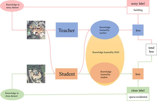
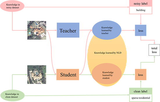
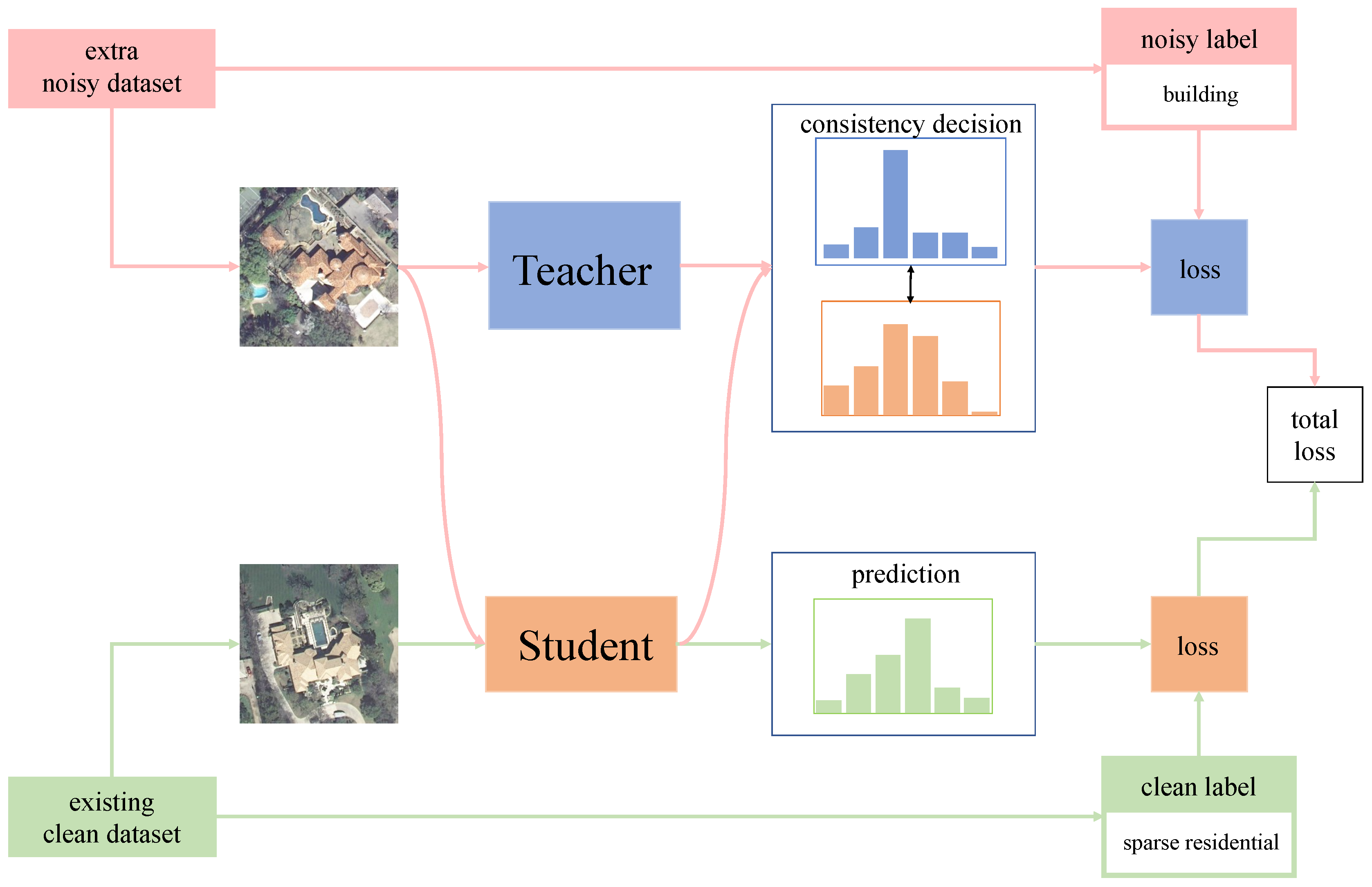
This work focuses on augmenting existing human-verified labeled datasets with additional noisy labeled data to improve the performance of remote sensing scene classifiers. A more efficient way is explored to learn knowledge from massive noise, instead of simply mix all data or fine-tuning with labeled images. Inspired by Deep Mutual Learning (DML) [19], this paper proposes a novel noisy label distillation framework called NLD based on teacher-student methodology with a decision network, as given in Figure 1. First, the student and teacher jointly learn from each other. Pre-training is no longer a required process. Second, the teacher distills the knowledge learned from noisy data to facilitate the student to learn from full dataset. NLD can even be applied to completely noise-free datasets. This means that our method can be used in a wide range of remote sensing applications. Third, a decision network derived from [20] is introduced, which is easier to optimize in practice and replace the calculation of the mimicry loss. Considering the lack of public datasets with noisy annotations for remote sensing image scene classification, experiments are conducted to evaluate NLD by injecting a series of noises into well-annotated datasets(e.g., UC Merced Land-use [21], NWPU-RESISC45 [22] and AID [23]).
Our contributions are as follows:
- Noise label is introduced for remote sensing image scene classification with minimal extra-human supervision. In practical applications, it is possible to label millions of images with noisy labels at a low-cost.
- A novel and effective end-to-end framework based on teacher-student model namely NLD is proposed for noisy labels distillation. NLD can effectively boost the performance of remote sensing scene classifiers with massive noisy annotations.
- NLD is effective on completely clean datasets. Thus, NLD can be further extended to model distillation for network compression.
- Pseudo-labeling methods can automatically generate nearly infinite noisy annotated images at no additional cost. The network trained by NLD achieves a better performance than other pseudo-labeling methods.
- Several new practical benchmarks are proposed for remote sensing image scene classification with different types of noisy labels.
2. Related Works
In this section, we will briefly review existing related works on remote sensing image scene classification and learning from noisy labels.
2.1. Remote Sensing Image Scene Classification
Remote sensing image scene classification aims to distinguish the semantic category of an image, which is a fundamental problem for understanding high-level geospatial information. With the development of deep learning methods, many CNN architectures (e.g., ResNet [24], VGG [25]) have achieved remarkable performance on many remote sensing public datasets. However, there are large intra-class variations and small inter-class dissimilarities between different remote sensing scenes. These problems will decrease the recognition abilities of models for some categories. To address these challenges, many studies focus on how to learn discriminative feature representations. Nogueira et al. [2] analyzed the use of different networks in the field of remote sensing. Chaib et al. [1] proposed an adequate method for feature fusion and introduced discriminant correlation analysis to represent the fused features. Zhang et al. [26] proposed a newly designed CapsNet to deal with the remote sensing image scene classification problem. Li et al. [27] proposed a unified feature fusion framework based on attention mechanism to improve the classification performance.
These algorithms are all data-driven algorithms, which means large-scale datasets are required in practice. To facilitate the application of these methods to more fields that have little data with clean annotations, NLD can be widely used with various models including the above research.
2.2. Learning from Noisy Labels
Most of methods learning from noisy datasets aim to directly learn without clean labels available. These approaches usually focus on noise-robust algorithms and label cleansing methods. Wang et al. [13] proposed symmetric cross entropy (SCE) loss to boost cross-entropy (CE) symmetrically with a noise-robust counterpart reverse CE. Northcutt et al. [14] proposed confident learning for characterizing, identifying, and learning with noisy labels. Kim et al. [15] proposed Selective Negative Learning and Positive Learning (SelNLPL) to filter and learn with noisy data. These methods face the problem of discriminating difficulty from mismatched labels.
Our approach belongs to a practical stream, assuming that both clean and noisy labels of the dataset are known [8,28]. This is a more practical scenario, allowing researchers to focus on leveraging noisy labeled data to enhance existing fully supervised algorithms. Veit et al. [16] proposed a learning approach for multi-label image classification using clean labeling combined with massive noise labeling. Hu et al. [18] proposed a method to automatically identify credible annotations in the massive noisy labels under weakly supervised learning. Many semi-supervised learning algorithms, especially pseudo-labeling algorithms, can also be categorized into such scenarios [29]. Han et al. [6] proposed a framework based on deep learning features, self-labeling techniques and decision evaluation methods under semi-supervision for remote sensing image scene classification and annotating datasets. The works closer to ours comes from Li et al. [17] and Li et al. [30].To achieve noisy label learning, they proposed a teacher-student framework, which comes from knowledge distillation [31]. To take full use of the whole data space, traditional knowledge distillation and many other similar noise-robust methods use the student model to mimic the large pre-trained teacher model by providing training experiences. These experiences are called “dark knowledge”.
In practice, a smaller network with the same precision is needed because of the cost, i.e., a student network. However, due to the existence of noisy labels, even under the guidance or regularization of a powerful network pre-trained with clean data, small networks are still prone to overfit to noisy labels. This may even lose the knowledge of the original clean data.
3. Method
3.1. Problem Formulation
Our goal is to train a remote sensing scenes classifier using a dataset with automatically collected noise labels and a part of human-verified clean labels available. The source of noisy labels may come from collects from the web or predictions from models trained on clean data or other ways. Furthermore, the framework can be used for large-scale datasets with fully clean annotations to improve the performance of networks under traditional supervised learning.
Formally, we define the notations for our study. Let donates the entire large training dataset, where is the clean subset and is the remaining noisy subset. In a single label classification problem, and , which contains and samples from M classes, respectively; and donate the label corresponding to image and . In this work, the ratio of to is not limited, because NLD can improve the performance of classifiers in different practical applications.
As shown in Figure 2, NLD is formulated with a cohort of two classifiers g and h. The classifier g is the large teacher model that is used to distill and transfer the knowledge of noise. In addition, its backbone is a powerful network such as a ResNet-50 [24]. The student model h is designed to learn from the clean labels and guided the learning process by the knowledge of noise which is distilled from the teacher network T. The network S is a network that is same as or shallower than network T (e.g., ResNet-34 [24] and VGG-16 [25]). The logits for given by the teacher network T can be represented as
where the is a nonlinear transformation in teacher network T. Similarly, the logits and can be represented as
where the is a nonlinear transformation in student network S.
For classifier g and h, the supervision depends on the source of the training sample. For image from the noisy dataset , the classifier g is supervised by the noisy label . For sample from the clean dataset , supervision comes directly from the verified label .
3.2. Noisy Distillation
In contrast to the previous work on teacher-student models including [17,30], we need to pre-train a teacher model with a small part of or the entire dataset: the teacher model and student model are trained together to learn latent noisy label distributions to improve the performance of student network supervised with the clean subset. NLD is motivated by DML which leverages a teacher-student framework to improve the representation of the network. The details will be analyzed in the later part of this section.
The student network learns the knowledge of clean data and acquires the distilled knowledge of the noisy dataset. The teacher takes advantage of powerful deep network architectures to learn features of noisy labels at various levels of abstraction rather than simply memorizing these. Besides, noise knowledge is distilled by comparing the outputs of the student and teacher simultaneously. To that end, the student and teacher model are trained by a mutual learning approach which originates from knowledge distillation. Noted that NLD is different from DML and other similar approaches. To match noisy label distributions, a metric between two branch’s representation vectors and needs to be defined. As a loss function, Kullback Leibler (KL) Divergence is the most widely used. The KL distance from and is computed as
where the is the score of class m in logits and the is the score of class m in logits .
According to the formula, KL divergence is asymmetric. Hence, the KL distance between the two networks is different. One can instead use a symmetric KL-divergence such as
Compared to teacher network T, student network S has similar representation capacities, but it is harder to learn appropriate parameters. In DML and other similar knowledge distillation algorithms, both teacher network and student network are trained on clean datasets. These studies expect the student network to mimic the classification probabilities and feature representations of the teacher network. The objective functions of the two networks are the same. Therefore, a simple combination of CE loss and KL divergence can facilitate a better student network from the entire clean dataset. However, how to combine and optimize these two different kinds of losses will be a difficult problem in our tasks. Our teacher network T is supervised by noise labels and our student network S is supervised by clean labels. The student network S should not totally mimic outputs of the teacher network T. By imitating and comparing, the purpose is to distill the knowledge from the noisy dataset, which is the intersection of clean student’s features and noisy teacher’s features. In the meanwhile, as mentioned above, a simple combination of CE loss and KL divergence would work on two networks identical to each other. Although this can be changed by adding some weights before the combination, there are too many options for hyper-parameters.
To address these problems, NLD feeds outputs of the two networks simultaneously into a decision network derived from [20]. The decision network simply consists of fully connected layers with a single output. In [20], this network is used to measure the similarity between two different images with siamese network. As discussed above, NLD has different settings from images similarity measurement methods. Different logits of two same image patches are mapping from different networks. Furthermore, the similarity of two networks is measured through the decision network. In addition, the decision network has learnable parameters. Instead of relying on the combination of different loss functions with hyper-parameters, this can automatically learn weights that fit the noisy label knowledge distillation. Because the original logits are mapping from the same image, the output r of decision network is still the original image feature mapping. The probability of class m for sample given by decision network is computed as
Subsequently, the classifier g is supervised by noisy labels and the classifier h is supervised by clean labels. In this way, the student network can learn clean knowledge and similar knowledge between clean labels and noise labels, i.e., noise distillation. At the same time, NLD does not need a mimicry loss, so training is faster and more flexible than traditional distillation methods. In the meanwhile, the decision network also increases inference time as it requires combinations of two vectors. However, our goal is to train a student network guided by the teacher network. Therefore, only the student network is used for testing, while the decision network is not used.
3.3. Model Training
In original knowledge distillation and DML, the whole objective function consists of a supervised loss (e.g., CE loss) and a mimicry loss(e.g., KL divergence). In contrast, CE loss is used as the supervised loss for classifier g and h, respectively. In addition, they can be rewritten as:
where and are the losses for the corresponding classifier g and h, respectively. Given the above definitions, the overall loss for the proposed model is constructed by two losses as follows:
where and denote weight factors that need to be set based on student network, teacher network and noisy dataset.
Training a network with a noisy dataset can lead the network to memorize these noises. To avoid the teacher network overfitting on noisy data, which will deteriorate the performance of noise distillation and may even mislead the student to have exploding gradients, batch normalization(BN) [32] and dropout layer [33] with a constant probability of 0.6 are applied between the teacher network and the decision network.
3.4. Extension to Pseudo-Labeling
Semi-supervised learning requires a small amount of manually labeled clean data, which is consistent with NLD. However, semi-supervised learning datasets usually contain a small amount of labeled data and a large amount of unlabeled data. Because NLD does not use additional mimicry loss, unlabeled data cannot be used directly. Pseudo-labeling belongs to the self-learning scenario which is often used in semi-supervised learning. Under the self-training settings, pseudo-labels are obtained by predicting unlabeled data through the models trained on labeled data. Some of the pseudo-labels will be mislabeled. These data with the pseudo-labels can be treated as a large noisy dataset and NLD can extend to semi-supervised learning.
Following [6], the pseudo-labeling method used is illustrated in Figure 3, which is close to traditional co-training. Denote the labelled and unlabeled subsets as and , where the entire training dataset is . First, there are two different classifiers and trained on the small labeled dataset , respectively. Given a batch of unlabeled images , two predictions and are provided by the classifiers and . Then, and can be represented as
Only when = , the predictions of the classifiers and will be regarded as the pseudo-label corresponding to , and other different results will be discarded. Apparently, this process will reduce the dataset size from , which typically affects the final performance. In fact, it removes low confidence predictions from pseudo-labels and reduces the noise level of the labels. High-quality pseudo-labels can improve performance and the robustness of the model. Furthermore, it does not need to choose a confidence threshold or manual selection. This is a more efficient pseudo-labeling method.
4. Experiments
In this section, we explain how to construct the mimic noisy datasets and describe the experimental details of our comparison with other methods on these datasets and evaluate NLD.
4.1. Datasets and Settings
4.1.1. Datasets
UC Merced Land-use dataset is a classical land-use dataset, which contains 21 different scenes and 2100 images. Each image has pixels and high-resolution in RGB color space with a spatial resolution of 0.3 m. They were all manually extracted from the USGS National Map Urban Area Imagery Collection.
NWPU-RESISC45 dataset has a total number of 45 scene classes and 700 images with a size of for each class. Most of the images are middle to high spatial resolution, which varies from 30 m to 0.2 m. They are all cropped from Google Earth. The dataset takes eight popular classes from UC Merced Land-use dataset and some widely used scene categories from other datasets and research.
AID is a large-scale aerial image dataset with 30 aerial scene types. The dataset is composed of 10,000 images which are multi-resolution and multi-source. The size of each image is fixed to be . The number of images in each class is imbalanced. This dataset is challenging because of the large intra-class diversities.
These datasets have many overlapped classes (e.g., sparse residential, medium residential and dense residential) that can easily confuse non-expert. It is particularly challenging for computer vision researchers with little geography knowledge to label such a dataset manually. As for crowd-sourcing or automatic labeling, it will be more prone to make errors. Actually, based on the existing public datasets, when we need to use them in real-world applications, additional data will be used. Only experts can avoid label noise, which is expensive.
Experiments are conducted on these three datasets. In addition, as shown in Table 1, each dataset is randomly split into training subset, validation subset and test subset. Because the existing datasets lack noisy labels, simulated approaches are taken to evaluate NLD. Three different types of noise are injected into the split training set of all the three datasets separately.
Symmetric noise: The symmetric noise is a type of uniform noise, which is generated by a random label among the classes to replace the ground-truth label with equal probabilities. This type of noisy subset represents an almost zero-cost annotation method, which means there are many unlabeled images, and labels are labeled in a completely random way. Experiments on this noise can prove that, through NLD, this labeling method is also feasible in some extremely low-cost scenarios.
Asymmetric noise: This type of noise is class dependent noise and it mimics some of the real-world noise for visually similar and semantically similar categories.
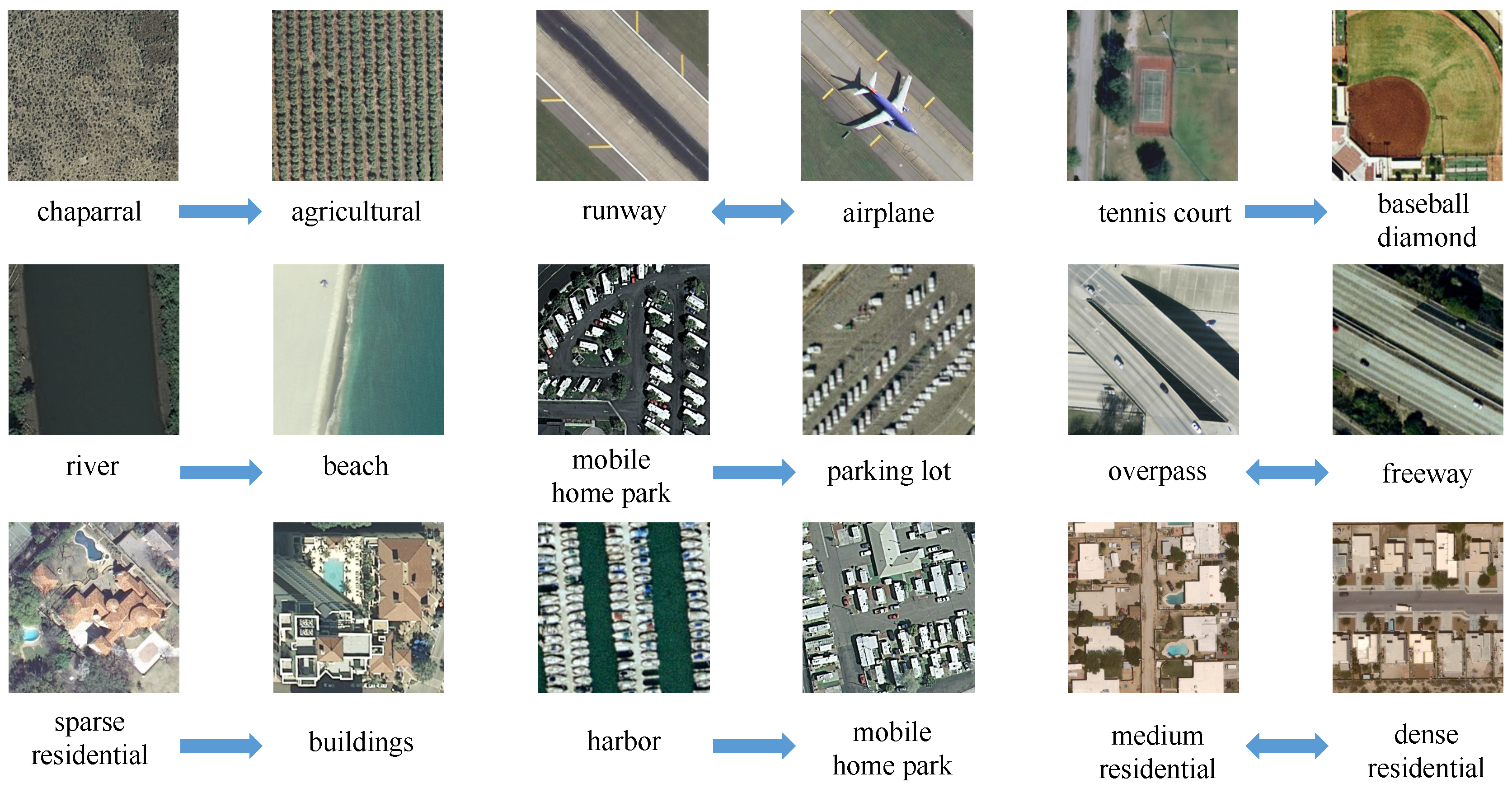
For UC Merced Land-use, to the best of our knowledge, there is no related noise label mapping method before. After observing the features of images and division of scene classes, asymmetric noise was generated by mapping , , , , , , , , as shown in Figure 4.
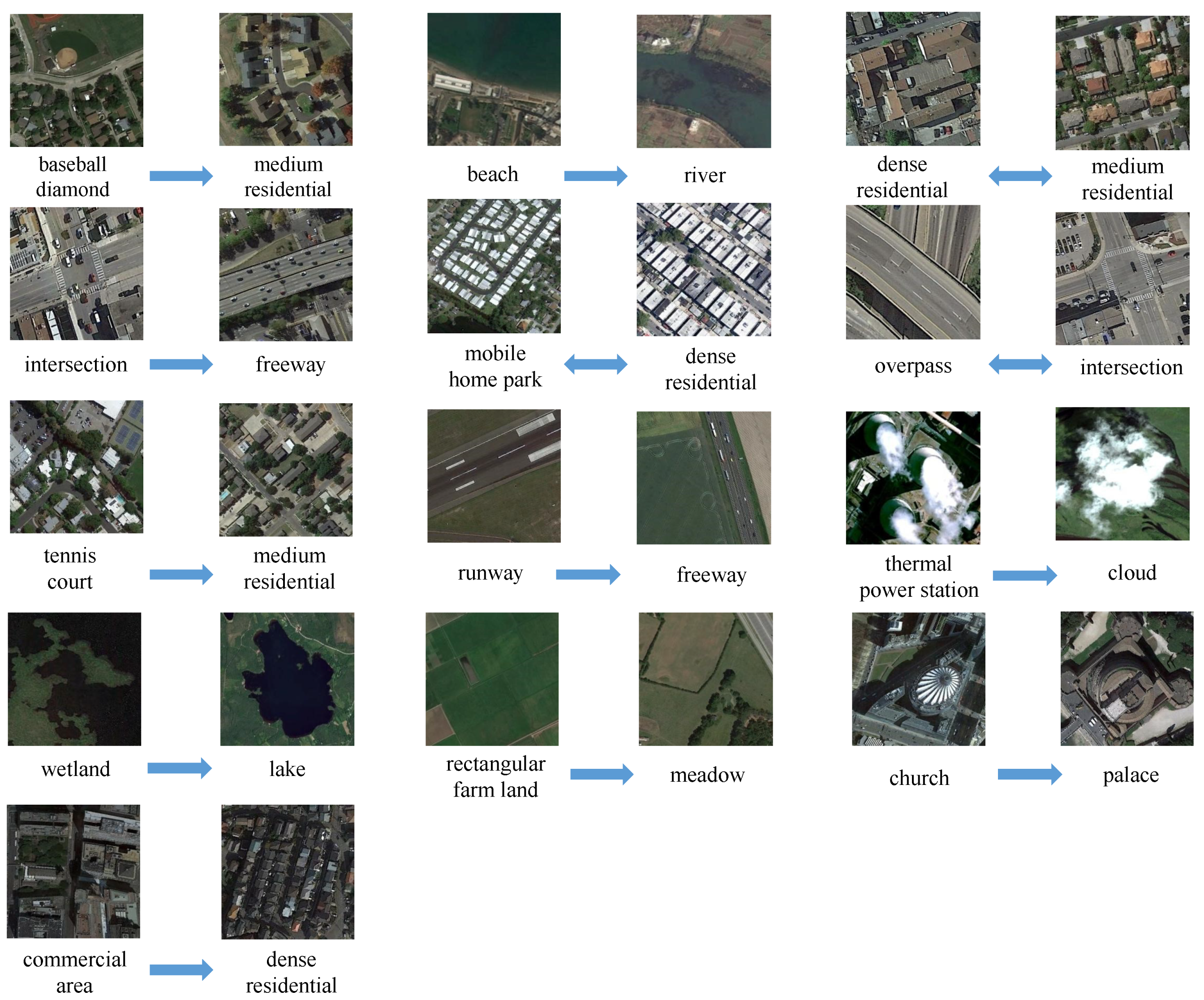
For NWPU-RESISC45, , , , , , , , , , , , , are mapped, following [12]. Figure 5 shows representative images in this dataset.
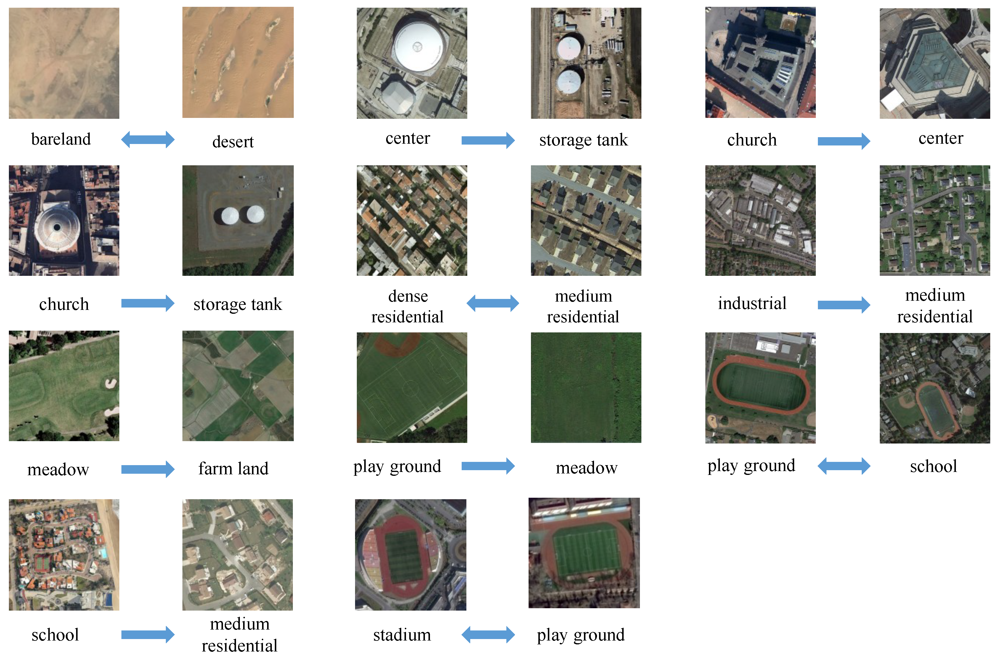
For AID, the classes are flipped by mapping ; ; ; ; ; ; ; ; ; , following [12]. Figure 6 shows examples from this dataset.
Pseudo-Labeling noise: Pseudo-labeling methods can assign labels to unlabeled images automatically, which can reduce costs. However, there are not completely correct pseudo-labels. To ensure a fair comparison, following the idea of SSGA-E [6], the full training set is randomly divided into six parts and randomly select one of them as a small clean subset. Then, two different classifiers are trained on the small clean subset and make pseudo labels for the rest of the train set. In SSGA-E [6], two networks are ResNet-50 and VGG-S [34], respectively. However, VGG-S is rarely used in practice, which can cause many problems in deployment. As a result, VGG-S is replaced with the VGG-19 [25], which has lower accuracy but is more widely used. These unlabeled subsets with automatically generated labels can be viewed as the noisy subset. In addition, since this method does not label all images, some of the uncertain images are removed from the subset and the noise subset will be smaller than the original subset. The number of annotations obtained for unlabeled images of different datasets is listed in Table 2.
4.1.2. Baselines and Model Variants
To evaluate the performance improvement of NLD, our approach is compared with some pseudo-labeling methods [6]. Several related baselines are also provided for symmetric noise, asymmetric noise. In addition, NLD is used as the base model for some other variants to verify the effectiveness of NLD. The details of the baselines and variants are as follows.
Baseline-Clean: A backbone network of the student model is trained for remote sensing scenes classification using the clean subset. This can be regarded as the lower bound of NLD. Our method uses the noisy subset to improve performance on this baseline.
Baseline-Noise: A backbone network of the student model is trained solely on noisy labels from the training set. This baseline can be viewed as a measurement of the quality of noisy labels.
Baseline-Mix: A backbone network of the student model is trained using a mix of clean and noisy labels with standard CE loss. This baseline shows the damage caused by noisy subsets.
SCE Loss: Under the supervision of SCE loss, a model is trained on the entire dataset with both clean and noisy labels. Parameters for SCE are configured as and .This is a baseline for a noise-robust method.
Noise model fine-tune with clean labels (Clean-FT): It is a common approach, which uses the clean subset directly to fine-tune the whole network of Baseline-Noise. This method is prone to overfit if there are few clean samples.
Noise model fine-tune with mix of clean and noisy labels (Mix-FT): To address the problem caused by limited clean labels, fine-tuning the Baseline-Noise with mixed data is also a common approach.
NLD with CE loss (NLD): NLD is trained on both the original clean datasets and different noisy ratios of datasets. For a completely clean dataset, one image is used as input simultaneously for the teacher and student, which is close to DML.
4.1.3. Experimental Settings
All experiments are implemented with PyTorch framework [35] and conducted on an NVIDIA GeForce Titan X GPU. The networks used in our experiments are shown in Table 3. These networks are all pre-trained on ImageNet. Although VGG architecture has a larger number of parameters and needs more floating point operations(FLOPs), ResNet architecture has stronger feature representation capabilities-based residual modules. Therefore, teacher networks in all experiments are ResNet architecture. For UC Merced Land-use dataset, it is worth mentioning that SSGA-E [6] uses VGG-S and VGG-16, but after our experiments, the network with VGG architectures will be over-fitting because the size of this dataset is small. So the actual network used is modified VGG architectures with BN to learn this dataset. As a preprocessing step, random flip, random gaussian blur and resize images to are used. For optimization, we use Adam with weight decay of , batch size of 32 and initial learning rate of . The leaning rate will decrease according to the exponential decay with the multiplicative factor of in each epoch. All networks mentioned in Section 4.1.2 are trained for 200 epochs. Besides, for NLD, a batch of images is half clean and half noise. In general, the weight factors are set to and . For additional experiments, experiments are conducted with more different factors, losses and networks, which will be detailed in Section 4.6
4.2. Results on UC Merced Land-Use
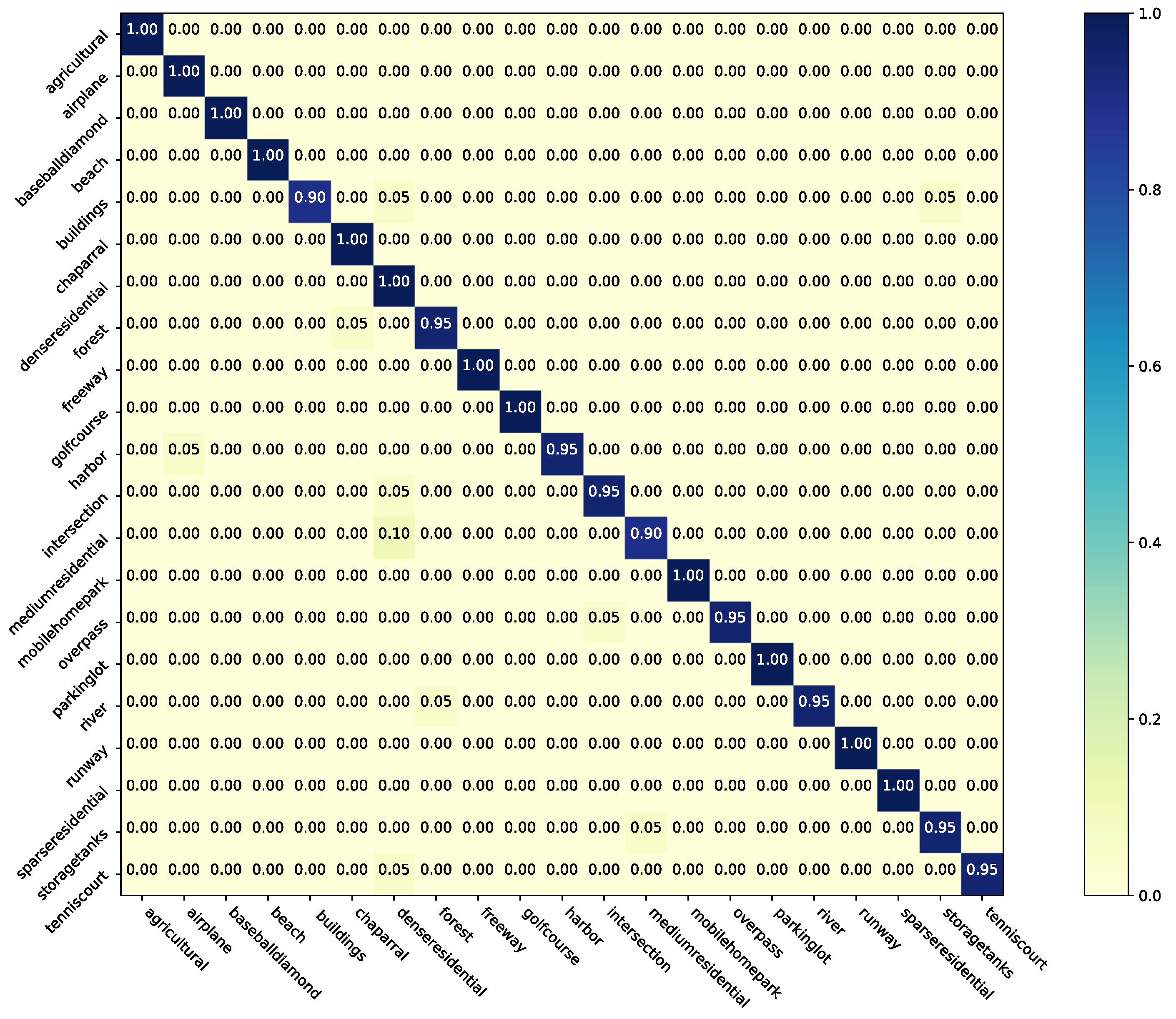
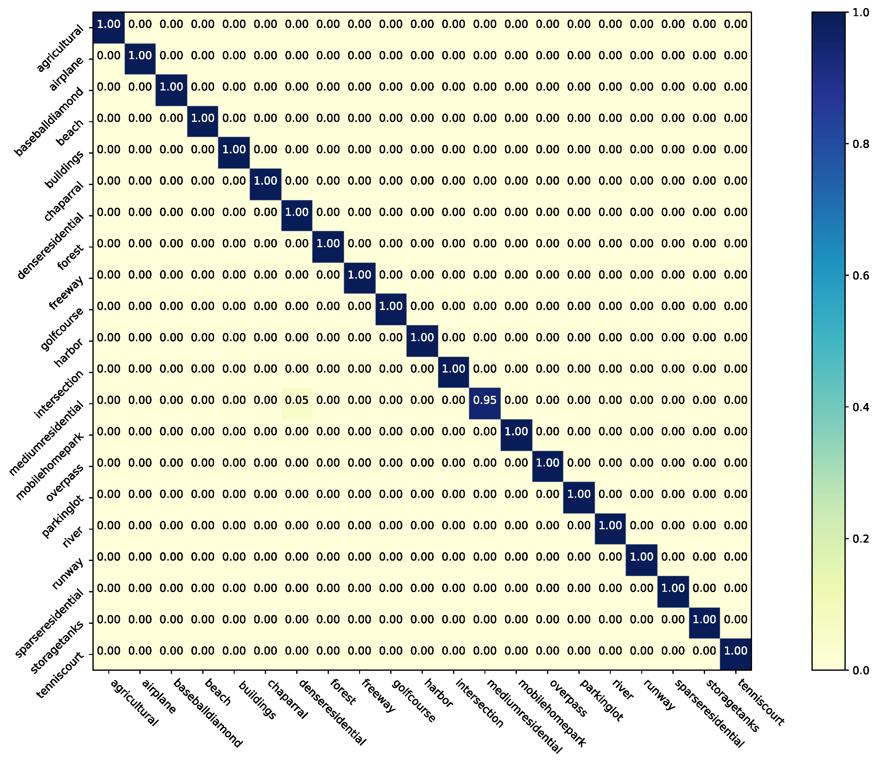
The results on the original UC Merced Land-use without any label noise and the UC Merced Land-use with symmetric label noise are reported in Table 4. Two confusion matrices for noise-free UC Merced Land-use are shown in Figure 7 and Figure 8, respectively. It is noticeable that the student network (ResNet-34) can significantly benefit for NLD when learning from the original noise-free dataset. Therefore, NLD can also be regarded as a model distillation-like process, without additional data and pre-trained models. For symmetric noise, this type of noise label is completely random and there is little correct information for NLD distilling the knowledge in the noisy subset. Our method can still make better performance and robustness of the student network in most cases. As for and cases, it revealed that when the clean subset or noisy subset is too small (e.g., 252 samples), clean labels or randomly generated labels are too weak to bootstrap the performance. Instead of improving performance, other common approaches even hurt the performance. When the label quality of the noise subset is extremely low, a lot of error guidance will be provided. Specifically, different fine-tuning methods require a pre-trained model of the noise subset, which may get worse initialization values than the ImageNet [3] pre-trained model. If the two subsets are mixed, the noise labels will become adversarial examples, which confuse the network. SCE or other noise-robust methods can alleviate this problem, but the performance is still far from the method with a small number of clean labels available.
Table 5 shows the results for asymmetric label noise. This noise is closer to the real scene, similar to crowd-sourcing labeling or crawling data from Internet. According to the results of Baseline-Noise, such labels can provide a more valuable pre-trained model than labels with symmetric noise. Clean-FT and Mix-FT provide clear improvements compared to Baseline-Clean and Baseline-Mix, respectively. However, for mix-based methods, during training, the learning process of the model on the clean subset will be continuously misguided by the noise labels. As the noise ratio increases and clean ratio decreases, less clean data is difficult to fight against more noisy data, the performance of Mix-FT and SCE Loss is severely impaired. For NLD, the framework can maintain a better performance with fewer clean labels and more noisy labels. When goes from to , the performance of the model will only decrease by . It is particularly noteworthy that when , NLD can exceed of the Baseline-Clean.
4.3. Results on NWPU-RESISC45
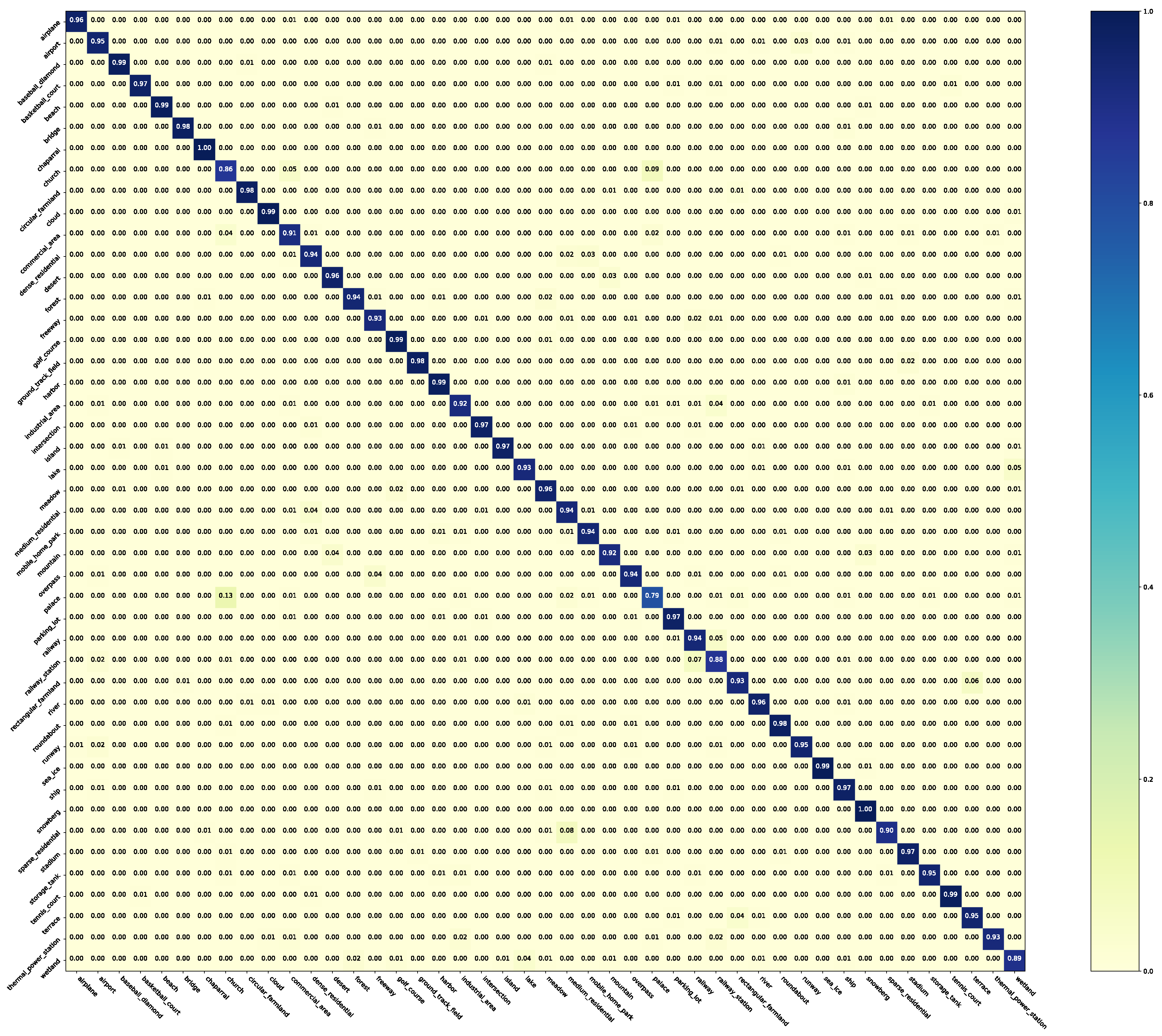
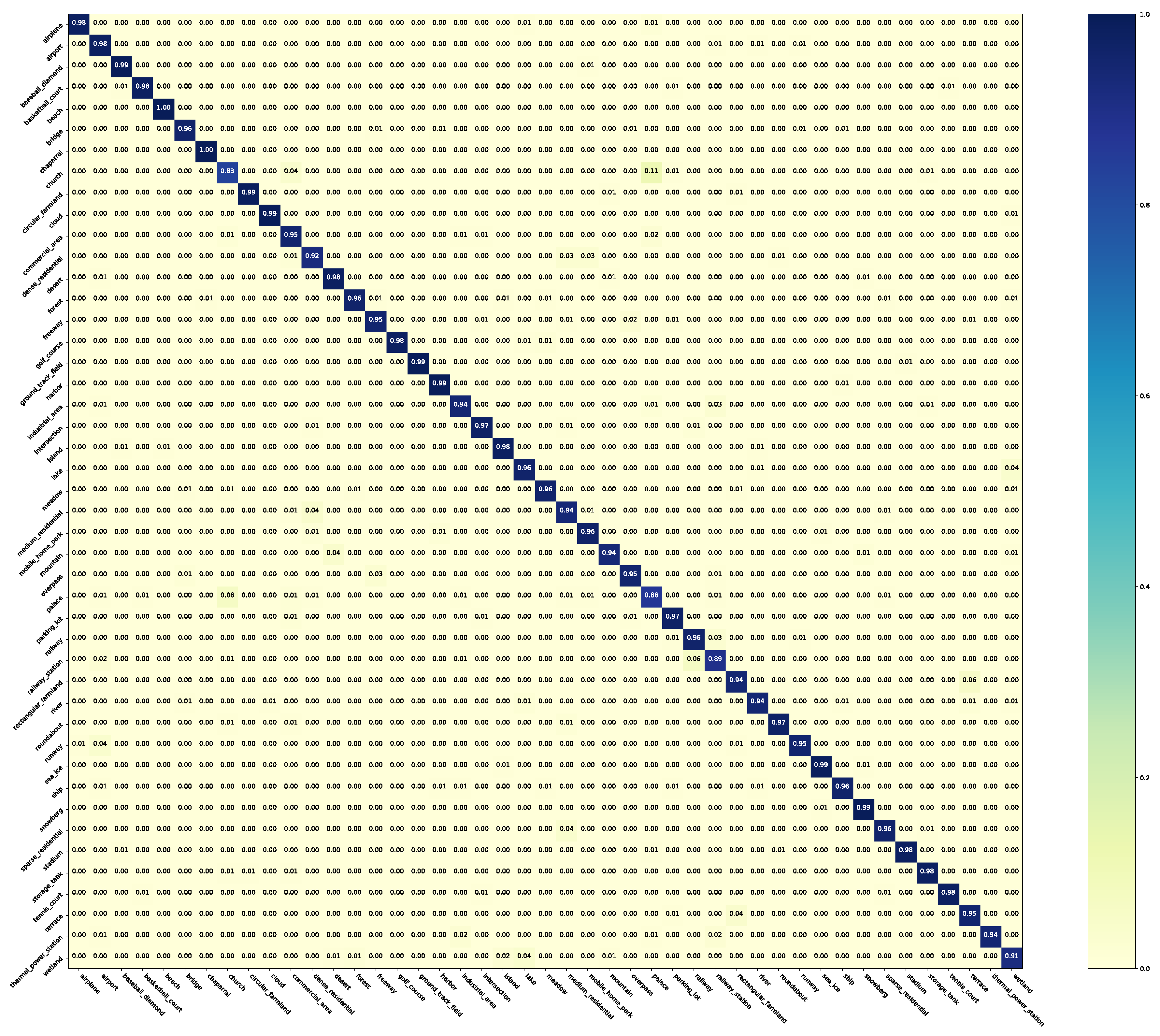
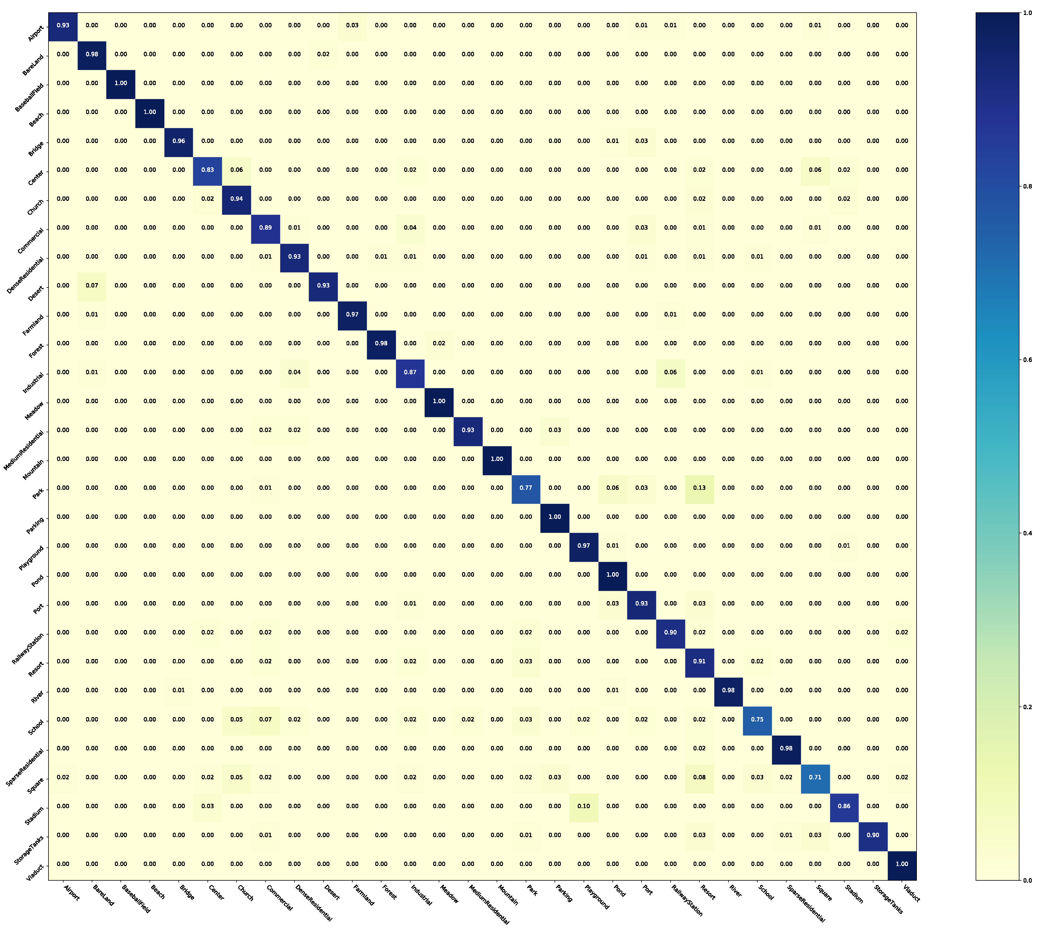
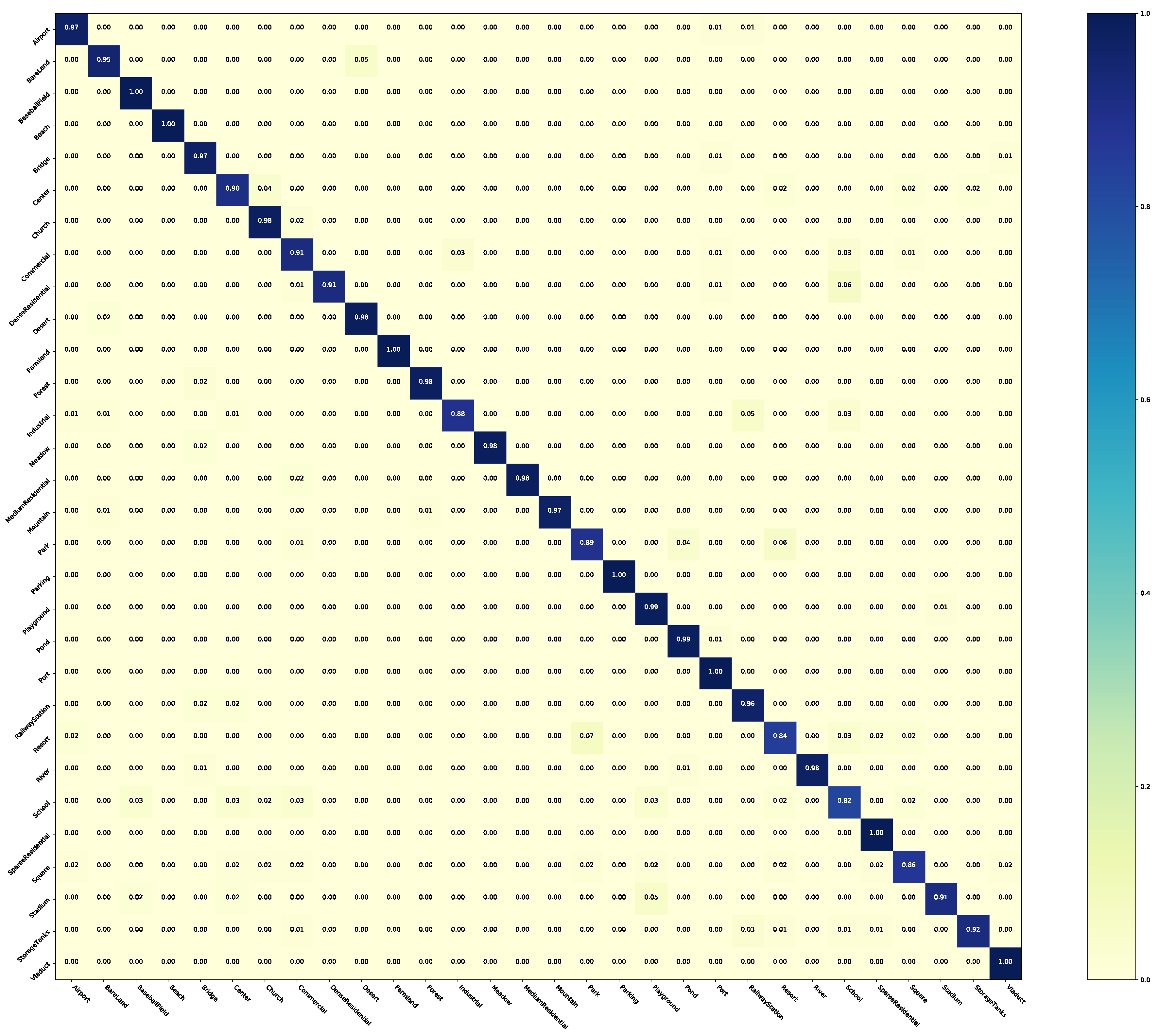
In this experiment, NLD is tested on NWPU-RESISC45 with different noisy types. Table 6 summarizes the classification accuracy (%) of ResNet-34 trained with/without NLD. According to Baseline-Noise, asymmetric noise can provide more correct information due to the larger scale of NWPU-RESISC45 than UC Merced Land-use. Thus, Clean-FT can benefit from asymmetric noisy labels. However, the performance of other methods is still compromised by the noise. On the contrary, NLD has strong robustness and can benefit from different ratios and types of noisy labels. As for the test set accuracy, NLD has clearly improved the baseline and direct fine-tuning. Figure 9 and Figure 10 show the confusion matrices of NLD and Baseline-Clean on original NWPU-RESISC45. It can be observed that NLD improves the performance of the student network as a method of model distillation.
4.4. Results on AID
Next, the performance of NLD is evaluated on the AID dataset. Table 7 shows the results. As the classes of AID are imbalanced, it is more challenge using noise labels. It can be observed that all methods are significantly affected by symmetric noise, especially when the noise rate increases. In contrast, asymmetric noise can change the imbalance of the data distribution. As a result, NLD can benefit from asymmetric noisy labels and improve performance. The gap between NLD and Clean-Baseline became especially apparent when the noise rate increased to larger values. Our method can be applied to scenarios with more noisy labels. For example, when the asymmetric noise rate is , NLD obtains higher accuracy than Baseline-Clean and higher than Clean-FT. The confusion matrices for the AID dataset with asymmetric noise of are shown in Figure 11 and Figure 12. The results of NLD are significantly better than Baseline-Clean.
4.5. Comparison with Pseudo-Labeling
We explore pseudo-labeling in UC Merced Land-use, NWPU-RESISC45 and AID. For all datasets, one-sixth of the training images per class is randomly selected as labeled, and the rest of images is treated as unlabeled. Experiments are compared with three pseudo-labeling strategies: (1) traditional self-training with single network; (2) traditional co-training with two networks respectively; (3) SSGA-E [6] with three networks.
Table 8 and Table 9 shows the result from Han et al. [6], supplemented with our results. NLD achieves the best overall accuracy in all cases. For the UC Merced Land-use, Resnet34 is more effective as a student network when there is less unlabeled data. When leveraging entire unlabeled subset, VGG-16 shows better performance as a student network. With a larger scale of labeled data (e.g., NWPU-RESISC45), the improvement of our framework is higher. This confirms that NLD benefits pseudo-labeling scenarios.
4.6. Additional Experiments
In this section, we study the importance of hyper-parameters and investigate the effect of changing components to provide additional insight into NLD.
Table 10 presents the following four experiments on UC Merced Land-use: (a) NLD with the weight factors and . (b) NLD with the weight factors and . (c) Using two same networks as student and teacher, respectively. (d) For the noisy teacher network, CE loss is replaced by SCE loss.
Hyper-parameters: From Table 10, hyper-parameters settings have a significant effect on the performance of NLD. As decreases and increases, the student network learns more information from noise distillation. Since the information in symmetric noise labels is limited, a larger cannot make the teacher network to distill more knowledge. In such cases, the network performance can be degraded by incorrect guidance. Similarly, asymmetric noise labels have more correct information. So a larger can enhance the teacher’s ability to distill the right instruction to the student. In the absence of noisy labels, the effect of factors is not significant. This result thus suggests that appropriate factors are needed to select based on the quality of the noise labels in practice.
Distillation with the same network: As shown in Table 10, we perform experiments for ResNet-34 as a teacher and a student. In general, the first thing to notice is that the teacher network with a smaller capacity can also benefit the student network. However, for noise-free scenarios, it cannot take effect because the teacher and student have the same input and architecture and it is difficult to get extra knowledge. Moreover, a larger standard deviation for most results implies worse robustness. Therefore, a large teacher network is still a better option. In some low-cost scenarios, it is also possible to choose a small teacher network.
Training teacher with different loss: SCE can supervise the network to learn more information in the noisy labels (i.e., more errors in symmetric noise or more correctness in asymmetric noise). For fully clean data, there is little additional benefit from SCE. Such a property produces the results in Table 10. Therefore, for most real applications, SCE should be used instead of CE for the teacher to achieve a better performance of NLD.
5. Conclusions
This work proposes an efficient framework named NLD to address the noisy label problem for remote sensing image scene classification. NLD can distill the knowledge from different types of noise to improve performance of networks. Teacher networks can avoid overfitting into the noise through consistent decisions with student networks. The decision network is introduced to replace KL divergence. It is different from previous methods for distillation. The proposed NLD framework is end-to-end and does not require a pre-training process besides ImageNet. Thus, NLD is more practical and easier to deploy.
NLD can fully leverage the information contained in the noisy labels to improve the performance of network trained on the clean labels. Experiments are conducted on UC Merced Land-use, NWPU-RESISC45 and AID with different noise types. NLD improves over the baseline and direct fine-tuning. It can also be easily extended to pseudo-labeling. NLD performs significantly better than SSGA-E and other methods. For completely clean datasets, NLD can also improve accuracy as a model distillation-like process.
Future work will explore real-world noise datasets. More data with noisy labels can be collected from search engines and google earth, etc. Furthermore, mixing multiple existing public datasets as a clean dataset is also a worthwhile experiment. Our goal is to apply NLD to real scenarios.
Author Contributions
Conceptualization, R.Z., Z.C. and T.L.; methodology, R.Z., Z.C. and T.L.; software, R.Z. and Z.C.; validation, R.Z., Z.C. and T.L.; formal analysis, R.Z. and F.S.; investigation, R.Z. and S.Z.; resources, T.L.; data curation, R.Z.; writing—original draft preparation, R.Z.; writing—review and editing, Z.C. and G.Z.; visualization, R.Z. and Q.Z.; supervision, T.L.; project administration, T.L.; funding acquisition, T.L. All authors have read and agreed to the published version of the manuscript.
Funding
This work was supported by Youth Innovation Promotion Association, Chinese Academy of Sciences (Grant No. 2016336).
Acknowledgments
The authors thank the editor and anonymous reviewers for their helpful comments and valuable suggestions.
Conflicts of Interest
The authors declare no conflict of interest.
Abbreviations
The following abbreviations are used in this manuscript:
| MDPI | Multidisciplinary Digital Publishing Institute |
| DOAJ | Directory of open access journals |
| TLA | Three letter acronym |
| LD | linear dichroism |
References
- Chaib, S.; Liu, H.; Gu, Y.; Yao, H. Deep feature fusion for VHR remote sensing scene classification. IEEE Trans. Geosci. Remote Sens. 2017, 55, 4775–4784. [Google Scholar] [CrossRef]
- Nogueira, K.; Penatti, O.A.; Dos Santos, J.A. Towards better exploiting convolutional neural networks for remote sensing scene classification. Pattern Recognit. 2017, 61, 539–556. [Google Scholar] [CrossRef] [Green Version]
- Deng, J.; Dong, W.; Socher, R.; Li, L.; Li, K.; Li, F. ImageNet: A large-scale hierarchical image database. In Proceedings of the 2009 IEEE Computer Society Conference on Computer Vision and Pattern Recognition (CVPR), Miami, FL, USA, 20–25 June 2009; IEEE Computer Society: Washington, DC, USA, 2009; pp. 248–255. [Google Scholar]
- Algan, G.; Ulusoy, I. Image Classification with Deep Learning in the Presence of Noisy Labels: A Survey. arXiv 2019, arXiv:1912.05170. [Google Scholar]
- Kuznetsova, A.; Rom, H.; Alldrin, N.; Uijlings, J.; Krasin, I.; Pont-Tuset, J.; Kamali, S.; Popov, S.; Malloci, M.; Duerig, T.; et al. The open images dataset v4: Unified image classification, object detection, and visual relationship detection at scale. arXiv 2018, arXiv:1811.00982. [Google Scholar] [CrossRef] [Green Version]
- Han, W.; Feng, R.; Wang, L.; Cheng, Y. A semi-supervised generative framework with deep learning features for high-resolution remote sensing image scene classification. ISPRS-J. Photogramm. Remote Sens. 2018, 145, 23–43. [Google Scholar] [CrossRef]
- Li, W.; Wang, L.; Li, W.; Agustsson, E.; Van Gool, L. Webvision database: Visual learning and understanding from web data. arXiv 2017, arXiv:1708.02862. [Google Scholar]
- Xiao, T.; Xia, T.; Yang, Y.; Huang, C.; Wang, X. Learning from massive noisy labeled data for image classification. In Proceedings of the IEEE Conference on Computer Vision and Pattern Recognition (CVPR), Boston, MA, USA, 7–12 June 2015; IEEE Computer Society: Washington, DC, USA, 2015; pp. 2691–2699. [Google Scholar]
- Lee, K.; He, X.; Zhang, L.; Yang, L. CleanNet: Transfer Learning for Scalable Image Classifier Training with Label Noise. In Proceedings of the 2018 IEEE Conference on Computer Vision and Pattern Recognition (CVPR), Salt Lake City, UT, USA, 18–22 June 2018; IEEE Computer Society: Washington, DC, USA, 2018; pp. 5447–5456. [Google Scholar]
- Jiang, J.; Ma, J.; Wang, Z.; Chen, C.; Liu, X. Hyperspectral image classification in the presence of noisy labels. IEEE Trans. Geosci. Remote Sens. 2018, 57, 851–865. [Google Scholar] [CrossRef] [Green Version]
- Tu, B.; Zhang, X.; Kang, X.; Wang, J.; Benediktsson, J.A. Spatial density peak clustering for hyperspectral image classification with noisy labels. IEEE Trans. Geosci. Remote Sens. 2019, 57, 5085–5097. [Google Scholar] [CrossRef]
- Damodaran, B.B.; Flamary, R.; Seguy, V.; Courty, N. An Entropic Optimal Transport loss for learning deep neural networks under label noise in remote sensing images. Comput. Vis. Image Underst. 2020, 191, 102863. [Google Scholar] [CrossRef] [Green Version]
- Wang, Y.; Ma, X.; Chen, Z.; Luo, Y.; Yi, J.; Bailey, J. Symmetric Cross Entropy for Robust Learning with Noisy Labels. In Proceedings of the 2019 IEEE/CVF International Conference on Computer Vision (ICCV), Seoul, Korea, 27 October–2 November 2019; IEEE: Piscataway, NJ, USA, 2019; pp. 322–330. [Google Scholar]
- Northcutt, C.G.; Jiang, L.; Chuang, I.L. Confident Learning: Estimating Uncertainty in Dataset Labels. arXiv 2019, arXiv:1911.00068. [Google Scholar]
- Kim, Y.; Yim, J.; Yun, J.; Kim, J. NLNL: Negative Learning for Noisy Labels. In Proceedings of the 2019 IEEE/CVF International Conference on Computer Vision (ICCV), Seoul, Korea, 27 October–2 November 2019; IEEE: Piscataway, NJ, USA, 2019; pp. 101–110. [Google Scholar]
- Veit, A.; Alldrin, N.; Chechik, G.; Krasin, I.; Gupta, A.; Belongie, S.J. Learning from Noisy Large-Scale Datasets with Minimal Supervision. In Proceedings of the 2017 IEEE Conference on Computer Vision and Pattern Recognition (CVPR), Honolulu, HI, USA, 21–26 July 2017; IEEE Computer Society: Washington, DC, USA, 2017; pp. 6575–6583. [Google Scholar]
- Li, Y.; Yang, J.; Song, Y.; Cao, L.; Luo, J.; Li, L. Learning from Noisy Labels with Distillation. In Proceedings of the IEEE International Conference on Computer Vision (ICCV), Venice, Italy, 22–29 October 2017; IEEE Computer Society: Washington, DC, USA, 2017; pp. 1928–1936. [Google Scholar]
- Hu, M.; Han, H.; Shan, S.; Chen, X. Weakly Supervised Image Classification Through Noise Regularization. In Proceedings of the IEEE Conference on Computer Vision and Pattern Recognition (CVPR), Long Beach, CA, USA, 16–20 June 2019; Computer Vision Foundation/IEEE: Piscataway, NJ, USA, 2019; pp. 11517–11525. [Google Scholar]
- Zhang, Y.; Xiang, T.; Hospedales, T.M.; Lu, H. Deep Mutual Learning. In Proceedings of the 2018 IEEE Conference on Computer Vision and Pattern Recognition (CVPR), Salt Lake City, UT, USA, 18–22 June 2018; IEEE Computer Society: Washington, DC, USA, 2018; pp. 4320–4328. [Google Scholar]
- Zagoruyko, S.; Komodakis, N. Learning to compare image patches via convolutional neural networks. In Proceedings of the IEEE Conference on Computer Vision and Pattern Recognition (CVPR), Boston, MA, USA, 7–12 June 2015; IEEE Computer Society: Washington, DC, USA, 2015; pp. 4353–4361. [Google Scholar]
- Yang, Y.; Newsam, S.D. Bag-of-visual-words and spatial extensions for land-use classification. In Proceedings of the 18th ACM SIGSPATIAL International Symposium on Advances in Geographic Information Systems (ACM-GIS), San Jose, CA, USA, 3–5 November 2010; Agrawal, D., Zhang, P., Abbadi, A.E., Mokbel, M.F., Eds.; ACM: New York, NY, USA, 2010; pp. 270–279. [Google Scholar]
- Cheng, G.; Han, J.; Lu, X. Remote sensing image scene classification: Benchmark and state of the art. Proc. IEEE 2017, 105, 1865–1883. [Google Scholar] [CrossRef] [Green Version]
- Xia, G.S.; Hu, J.; Hu, F.; Shi, B.; Bai, X.; Zhong, Y.; Zhang, L.; Lu, X. AID: A benchmark data set for performance evaluation of aerial scene classification. IEEE Trans. Geosci. Remote Sens. 2017, 55, 3965–3981. [Google Scholar] [CrossRef] [Green Version]
- He, K.; Zhang, X.; Ren, S.; Sun, J. Deep Residual Learning for Image Recognition. In Proceedings of the 2016 IEEE Conference on Computer Vision and Pattern Recognition (CVPR), Las Vegas, NV, USA, 27–30 June 2016; IEEE Computer Society: Washington, DC, USA, 2016; pp. 770–778. [Google Scholar]
- Simonyan, K.; Zisserman, A. Very deep convolutional networks for large-scale image recognition. arXiv 2014, arXiv:1409.1556. [Google Scholar]
- Zhang, W.; Tang, P.; Zhao, L. Remote sensing image scene classification using CNN-CapsNet. Remote Sens. 2019, 11, 494. [Google Scholar] [CrossRef] [Green Version]
- Li, J.; Lin, D.; Wang, Y.; Xu, G.; Zhang, Y.; Ding, C.; Zhou, Y. Deep Discriminative Representation Learning with Attention Map for Scene Classification. Remote Sens. 2020, 12, 1366. [Google Scholar] [CrossRef]
- Inoue, N.; Simo-Serra, E.; Yamasaki, T.; Ishikawa, H. Multi-label Fashion Image Classification with Minimal Human Supervision. In Proceedings of the 2017 IEEE International Conference on Computer Vision Workshops (ICCV Workshops), Venice, Italy, 22–29 October 2017; IEEE Computer Society: Washington, DC, USA, 2017; pp. 2261–2267. [Google Scholar]
- Sohn, K.; Berthelot, D.; Li, C.L.; Zhang, Z.; Carlini, N.; Cubuk, E.D.; Kurakin, A.; Zhang, H.; Raffel, C. Fixmatch: Simplifying semi-supervised learning with consistency and confidence. arXiv 2020, arXiv:2001.07685. [Google Scholar]
- Li, Q.; Peng, X.; Cao, L.; Du, W.; Xing, H.; Qiao, Y. Product Image Recognition with Guidance Learning and Noisy Supervision. arXiv 2019, arXiv:1907.11384. [Google Scholar]
- Hinton, G.; Vinyals, O.; Dean, J. Distilling the knowledge in a neural network. arXiv 2015, arXiv:1503.02531. [Google Scholar]
- Ioffe, S.; Szegedy, C. Batch normalization: Accelerating deep network training by reducing internal covariate shift. arXiv 2015, arXiv:1502.03167. [Google Scholar]
- Srivastava, N.; Hinton, G.; Krizhevsky, A.; Sutskever, I.; Salakhutdinov, R. Dropout: A simple way to prevent neural networks from overfitting. J. Mach. Learn. Res. 2014, 15, 1929–1958. [Google Scholar]
- Chatfield, K.; Simonyan, K.; Vedaldi, A.; Zisserman, A. Return of the devil in the details: Delving deep into convolutional nets. arXiv 2014, arXiv:1405.3531. [Google Scholar]
- Paszke, A.; Gross, S.; Massa, F.; Lerer, A.; Bradbury, J.; Chanan, G.; Killeen, T.; Lin, Z.; Gimelshein, N.; Antiga, L.; et al. PyTorch: An Imperative Style, High-Performance Deep Learning Library. In Proceedings of the Advances in Neural Information Processing Systems 32: Annual Conference on Neural Information Processing Systems 2019 (NeurIPS), Vancouver, BC, Canada, 8–14 December 2019; Wallach, H.M., Larochelle, H., Beygelzimer, A., d’Alché-Buc, F., Fox, E.B., Garnett, R., Eds.; Curran Associates, Inc.: Red Hook, NY, USA, 2019; pp. 8024–8035. [Google Scholar]
Figure 1.
A high-level illustration of NLD. The student and teacher mutually learn knowledge of clean and noisy labels.
Figure 1.
A high-level illustration of NLD. The student and teacher mutually learn knowledge of clean and noisy labels.

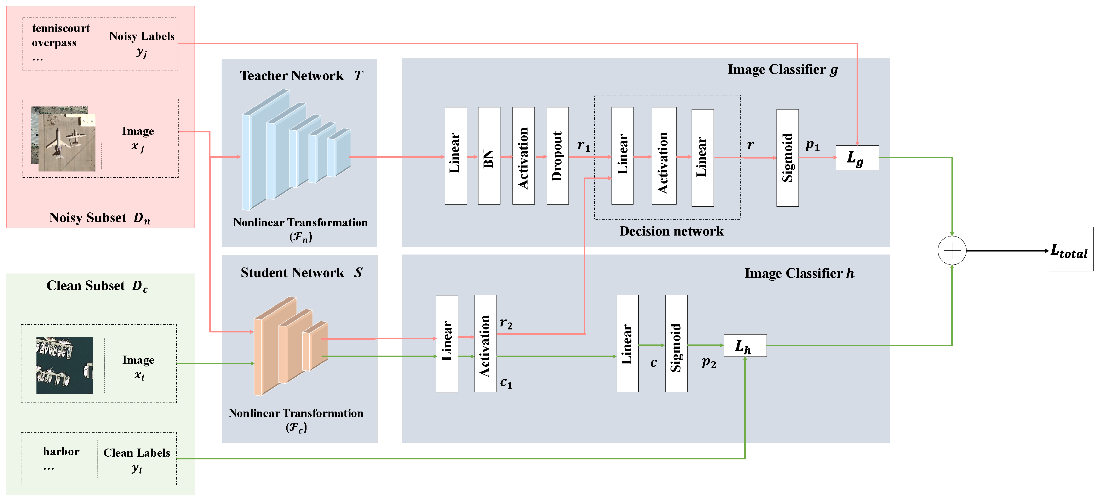
Figure 2.
The overview of the proposed framework to train a remote sensing scenes classifier from a large dataset with noisy labels and a small dataset with manually verified labels. The framework consists of teacher network T, student network S, decision network, fully connected layers, and predictor of softmax. In the training phase, two loss terms and (a CE loss with noisy labels and a CE loss with clean labels) are minimized jointly. The teacher model T transfers the “dark knowledge” distilled from noisy subset to the student model S through the decision network. In the inference phase, a classifier containing the student network S, fully connected layers and softmax can give the correct predictions.

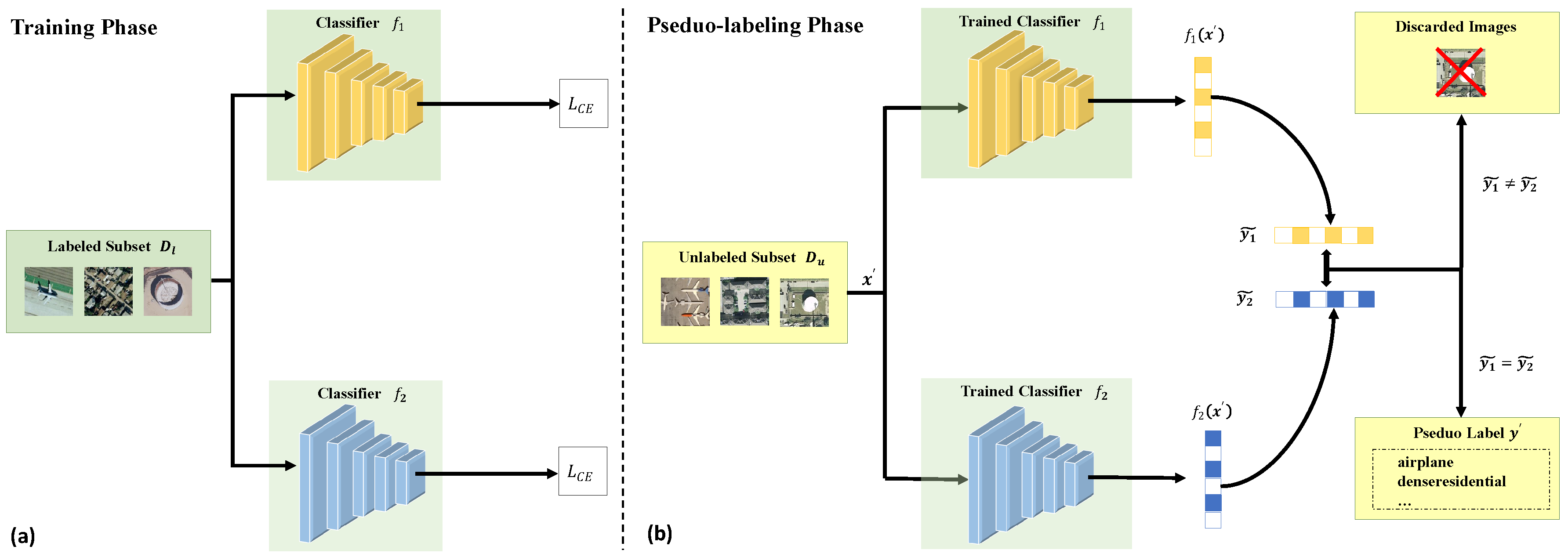
Figure 3.
Illustration of the pseudo-labeling method, which includes two phases: training two classifiers and pseudo-labeling. (a) Two different classifiers and trained on the small manually labeled subset , respectively. They provide two views of the data. (b) The trained models can predict labels on a batch of unlabeled data. When the inferences are the same, the predicted labels will remain as pseudo-labels for the corresponding images, and the rest will be discarded. donate CE loss. and represent the predictions of two classifiers, respectively. indicates pseudo-labels of the batch of images .

Figure 4.
Examples of asymmetric noise mapping scenes in the UC Merced Land-use dataset.

Figure 5.
Examples of asymmetric noise mapping scenes in the NWPU-RESISC45 dataset.

Figure 6.
Examples of asymmetric noise mapping scenes in the AID dataset.

Figure 7.
The confusion matrix of Baseline-Clean with full UC Merced Land-use dataset.

Figure 8.
The confusion matrix of NLD with full UC Merced Land-use dataset.

Figure 9.
The confusion matrix of Baseline-Clean for the NWPU-RESISC45.

Figure 10.
The confusion matrix of NLD for the NWPU-RESISC45.

Figure 11.
The confusion matrix of Baseline-Clean for the AID dataset with asymmetric noise of .

Figure 12.
The confusion matrix of NLD for the AID dataset with asymmetric noise of .


Table 1.
Sample sizes for different datasets.
| Datasets | Entire Dataset | Training Subset | Validation Subset | Test Subset |
|---|---|---|---|---|
| UC Merced Land-use | 2100 | 1260 | 420 | 420 |
| NWPU-RESISC45 | 31,500 | 18,900 | 6300 | 6300 |
| AID | 10,000 | 6000 | 2000 | 2000 |
Table 2.
Number of samples contained in different subsets. The unlabeled subset is of the entire training set. Pseudo-labeled subset is generated in unlabeled subset by the automatic labeling method trained with the clean labeled subset (i.e., of the entire training set) as a clean subset.
Table 2.
Number of samples contained in different subsets. The unlabeled subset is of the entire training set. Pseudo-labeled subset is generated in unlabeled subset by the automatic labeling method trained with the clean labeled subset (i.e., of the entire training set) as a clean subset.
| Datasets | Entire Training Subset | Clean Labeled Subset | Unlabeled Subset | Pseudo-Labeled Subset |
|---|---|---|---|---|
| UC Merced Land-use | 1260 | 210 | 1050 | 859 |
| NWPU-RESISC45 | 18,900 | 3150 | 15,750 | 13,625 |
| AID | 6000 | 1000 | 5000 | 4535 |
Table 3.
Comparison of various network architecture.
| Network Type | Million Parameters | GFLOPs |
|---|---|---|
| ResNet-34 | 21.819 | 3.679 |
| ResNet-50 | 25.578 | 4.136 |
| VGG-16 | 138.379 | 15.608 |
| VGG-16 with BN | 138.387 | 15.662 |
| VGG-19 | 143.688 | 19.771 |
| VGG-19 with BN | 143.699 | 19.830 |
Table 4.
Classification accuracy (%) on the UC Merced Land-use test set for different methods trained with the original noise-free dataset and symmetric label noise. We report the mean and standard error across 5 runs.
Table 4.
Classification accuracy (%) on the UC Merced Land-use test set for different methods trained with the original noise-free dataset and symmetric label noise. We report the mean and standard error across 5 runs.
| Methods | Network Types | None | Symm | |||
|---|---|---|---|---|---|---|
| 10 : 0 | 8 : 2 | 6 : 4 | 4 : 6 | 2 : 8 | ||
| Baseline-Clean | ResNet-34 | |||||
| Baseline-Noise | ResNet-34 | - | ||||
| Baseline-Mix | ResNet-34 | - | ||||
| SCE Loss | ResNet-34 | - | ||||
| Mix-FT | ResNet-34 | - | ||||
| Clean-FT | ResNet-34 | - | ||||
| NLD | ResNet-50+ResNet-34 | |||||
Table 5.
Classification accuracy (%) on the UC Merced Land-use test set for different methods trained with asymmetric label noise. We report the mean and standard error across 5 runs.
Table 5.
Classification accuracy (%) on the UC Merced Land-use test set for different methods trained with asymmetric label noise. We report the mean and standard error across 5 runs.
| Methods | Network Types | Asym | |||
|---|---|---|---|---|---|
| 8 : 2 | 6 : 4 | 4 : 6 | 2 : 8 | ||
| Baseline-Clean | ResNet-34 | ||||
| Baseline-Noise | ResNet-34 | ||||
| Baseline-Mix | ResNet-34 | ||||
| SCE Loss | ResNet-34 | ||||
| Mix-FT | ResNet-34 | ||||
| Clean-FT | ResNet-34 | ||||
| NLD | ResNet-50+ResNet-34 | ||||
Table 6.
Classification accuracy (%) on the NWPU-RESISC45 test set for different methods.
| Methods | Network Types | None | Symm | Asym | ||
|---|---|---|---|---|---|---|
| 10 : 0 | 6 : 4 | 4 : 6 | 4 : 6 | 2 : 8 | ||
| Baseline-Clean | ResNet-34 | |||||
| Baseline-Noise | ResNet-34 | - | ||||
| Mix-FT | ResNet-34 | - | ||||
| Clean-FT | ResNet-34 | - | ||||
| Ours | ResNet-50+ResNet-34 | |||||
Table 7.
Classification accuracy (%) on the AID test set for different methods.
| Methods | Network Types | None | Symm | Asym | ||
|---|---|---|---|---|---|---|
| 10 : 0 | 6 : 4 | 4 : 6 | 4 : 6 | 2 : 8 | ||
| Baseline-Clean | ResNet-34 | |||||
| Baseline-Noise | ResNet-34 | - | ||||
| Mix-FT | ResNet-34 | - | ||||
| Clean-FT | ResNet-34 | - | ||||
| NLD | ResNet-50+ResNet-34 | |||||
Table 8.
The effect of the unlabeled sample ratio on accuracy for the UC Merced Land-use test set reported by Han et al. [6], supplemented with our results.
Table 8.
The effect of the unlabeled sample ratio on accuracy for the UC Merced Land-use test set reported by Han et al. [6], supplemented with our results.
| Methods | Network Types | Unlabeled Samples | ||||
|---|---|---|---|---|---|---|
| 210 | 420 | 630 | 840 | 1050 | ||
| Self-training [6] | VGG-S | - | ||||
| ResNet50 | ||||||
| Co-training [6] | ResNet50&&VGG-S | |||||
| SSGA-E [6] | ResNet50&&VGG-S+VGG16 | |||||
| NLD | ResNet50&&VGG-19+ResNet50+VGG16 | |||||
| NLD | ResNet50&&VGG-19+ResNet50+ResNet34 | |||||
Table 9.
Comparison with results on the NWPU-RESISC45 and AID test set reported by Han et al. [6].
Table 9.
Comparison with results on the NWPU-RESISC45 and AID test set reported by Han et al. [6].
| Methods | Network Types | Dataset | |
|---|---|---|---|
| NWPU-RESISC45 | AID | ||
| Self-training [6] | VGG-S | 81.46 | 86.02 |
| ResNet-50 | 85.82 | 89.38 | |
| Co-training [6] | ResNet-50&&VGG-S | 87.25 | 90.87 |
| SSGA-E [6] | ResNet-50&&VGG-S+VGG-16 | 88.60 | 91.35 |
| NLD | ResNet-50&&VGG-19+ResNet-50+VGG16 | 91.35 | 92.65 |
Table 10.
Classification accuracy (%) on the UC Merced Land-use test set after changing each module from our model.
Table 10.
Classification accuracy (%) on the UC Merced Land-use test set after changing each module from our model.
| Network Types | Loss | None | Symm | Asym | |||
|---|---|---|---|---|---|---|---|
| 10 : 0 | 6 : 4 | 4 : 6 | 4 : 6 | 2 : 8 | |||
| ResNet-50+ResNet-34 | |||||||
| ResNet-50+ResNet-34 | |||||||
| ResNet-34+ResNet-34 | |||||||
| ResNet-50+ResNet-34 | |||||||
© 2020 by the authors. Licensee MDPI, Basel, Switzerland. This article is an open access article distributed under the terms and conditions of the Creative Commons Attribution (CC BY) license (http://creativecommons.org/licenses/by/4.0/).
Share and Cite
MDPI and ACS Style
Zhang, R.; Chen, Z.; Zhang, S.; Song, F.; Zhang, G.; Zhou, Q.; Lei, T. Remote Sensing Image Scene Classification with Noisy Label Distillation. Remote Sens. 2020, 12, 2376. https://0-doi-org.brum.beds.ac.uk/10.3390/rs12152376
AMA Style
Zhang R, Chen Z, Zhang S, Song F, Zhang G, Zhou Q, Lei T. Remote Sensing Image Scene Classification with Noisy Label Distillation. Remote Sensing. 2020; 12(15):2376. https://0-doi-org.brum.beds.ac.uk/10.3390/rs12152376
Chicago/Turabian StyleZhang, Rui, Zhenghao Chen, Sanxing Zhang, Fei Song, Gang Zhang, Quancheng Zhou, and Tao Lei. 2020. "Remote Sensing Image Scene Classification with Noisy Label Distillation" Remote Sensing 12, no. 15: 2376. https://0-doi-org.brum.beds.ac.uk/10.3390/rs12152376
Note that from the first issue of 2016, this journal uses article numbers instead of page numbers. See further details here.