Author Contributions
Conceptualization, L.W., M.M., S.H., R.T., J.P. and J.D.; Methodology, L.W., M.M., S.H., R.T., J.P. and J.D; Software, L.W. and M.M.; Validation, L.W., M.M., S.H., R.T., J.P. and J.D.; Formal Analysis, L.W., M.M., S.H., R.T., J.P. and J.D.; Investigation, L.W. and M.M.; Data curation, L.W., M.M.; Writing—Original Draft Preparation, L.W; Writing—Review and Editing, L.W., M.M., S.H., R.T., J.P. and J.D.; Visualization, L.W. and M.M; Project administration, L.W. All authors have read and agreed to the published version of the manuscript.
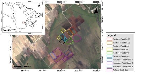
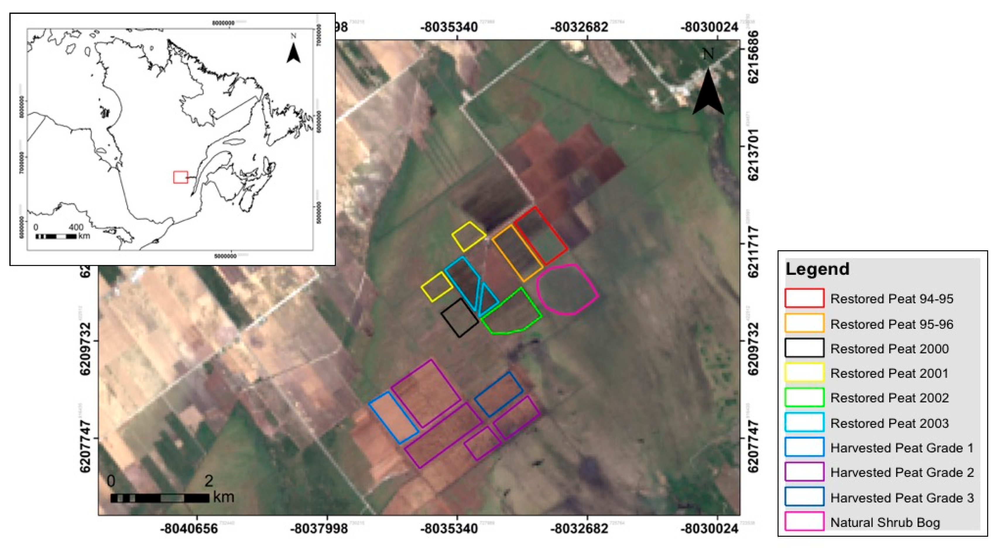
Figure 1.
Location map of the Sainte-Marguerite-Marie peatland in Quebec, Canada. The map on the top left shows the location of the Sainte-Marguerite-Marie peatland (red box) in relation to the rest of Quebec, Canada. The lower map shows a close-up view of the Sainte-Marguerite peatland with examples of restored peat from different years, different grades of harvested peat, and natural shrub bog, which were all included in the analysis for this research. The background is a Landsat-8 image.
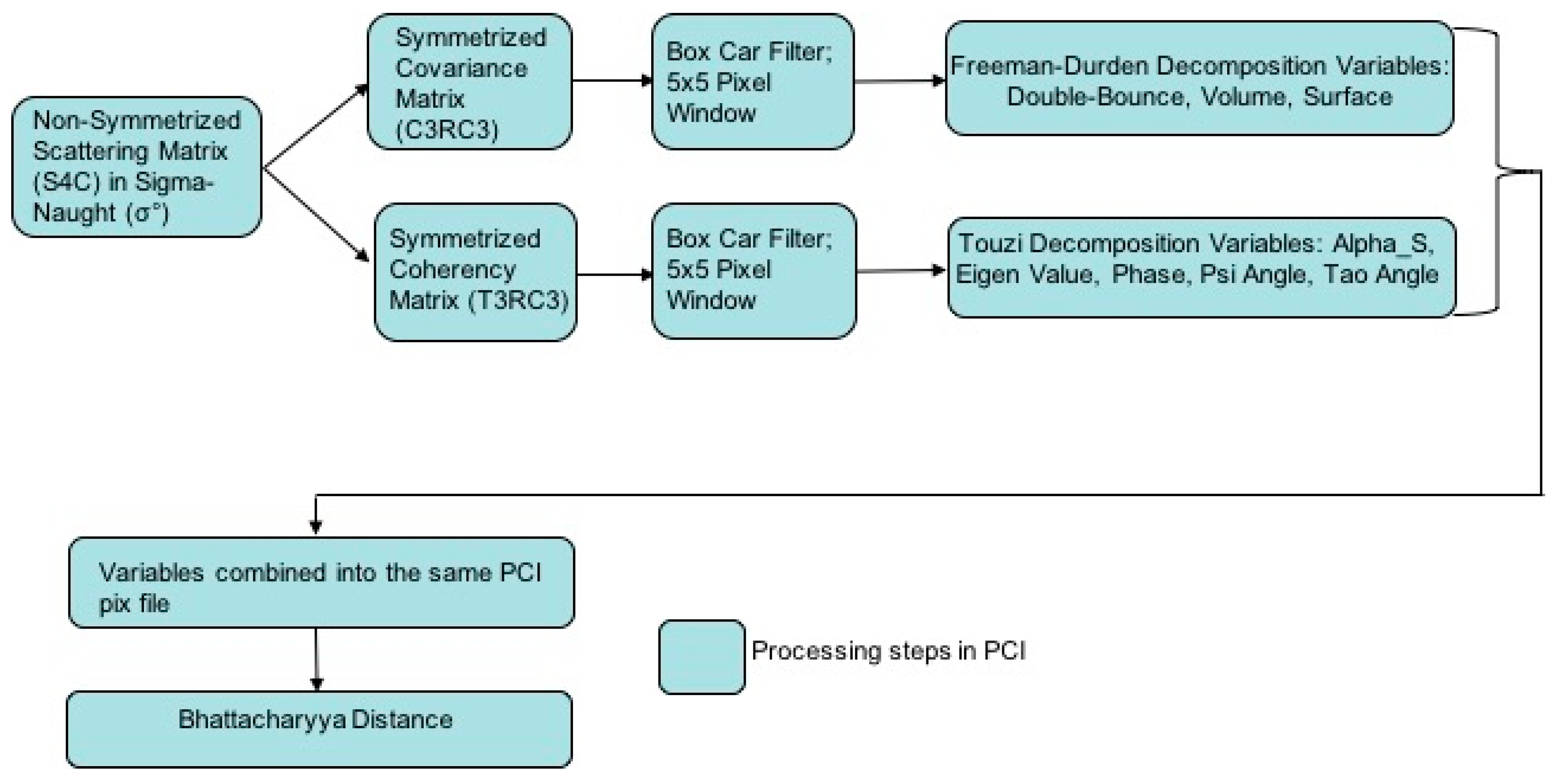
Figure 2.
PCI Geomatica Processing chain used to process the FD and the ICTD. The final step was to apply the Bhattacharyya Distance to determine the spectral signature separability between areas of peat that had been restored, peat which is currently being harvested, and natural shrub bog.
Figure 2.
PCI Geomatica Processing chain used to process the FD and the ICTD. The final step was to apply the Bhattacharyya Distance to determine the spectral signature separability between areas of peat that had been restored, peat which is currently being harvested, and natural shrub bog.
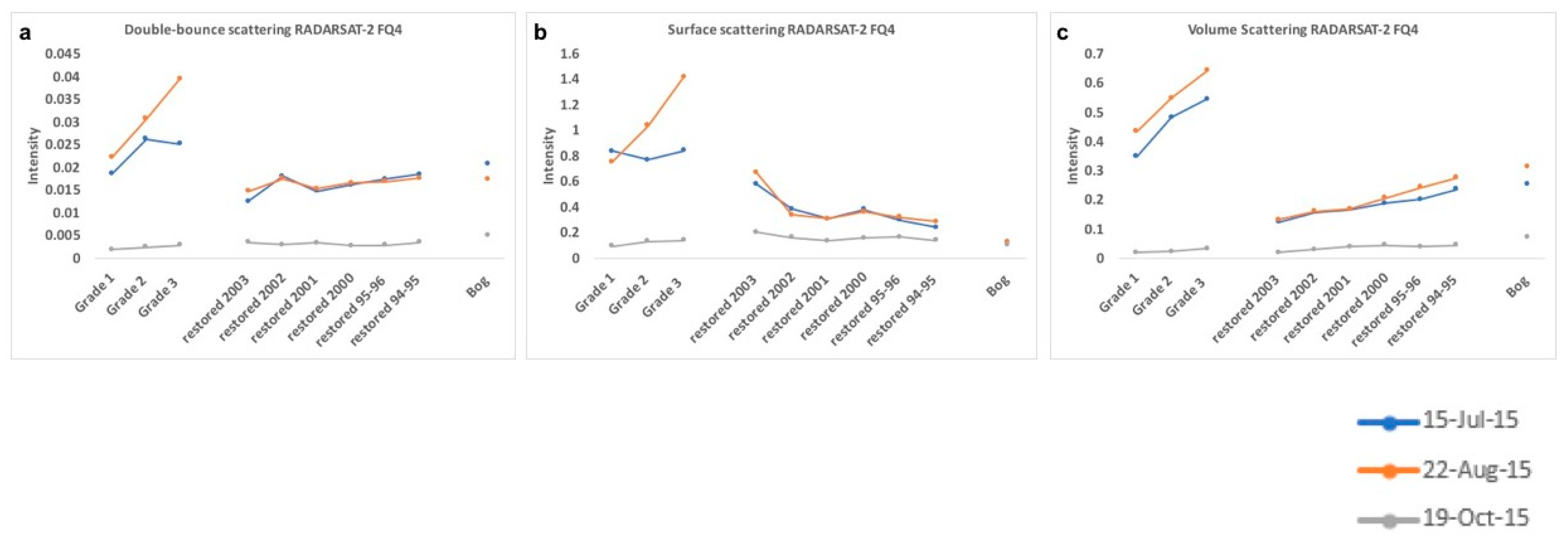
Figure 3.
The Freeman–Durden decomposition spectral signatures for natural shrub bog, restored peat, and harvested peat using RADARSAT-2 FQ4 imagery. Double-bounce scattering is presented in (a), surface scattering in (b), and volume scattering in (c). All values are represented in decibels (dB).
Figure 3.
The Freeman–Durden decomposition spectral signatures for natural shrub bog, restored peat, and harvested peat using RADARSAT-2 FQ4 imagery. Double-bounce scattering is presented in (a), surface scattering in (b), and volume scattering in (c). All values are represented in decibels (dB).
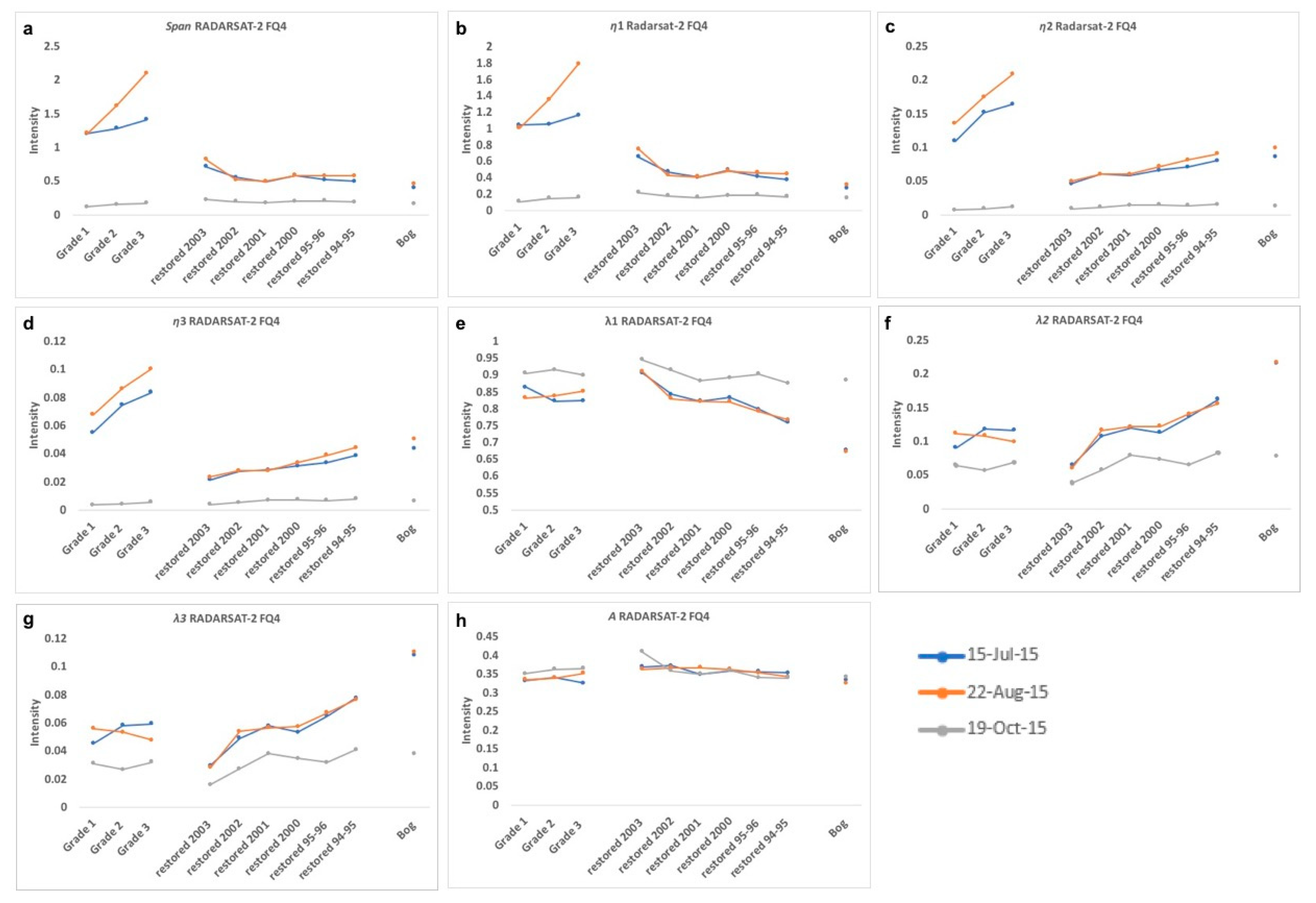
Figure 4.
RADARSAT-2 FQ4 spectral signatures for natural shrub bog, restored peat, and actively harvested peat. (a) Total power (span), (b) dominant eigenvalue, (c) secondary eigenvalue, (d) tertiary eigenvalue, (e) normalized dominant eigenvalue, (f) normalized secondary eigenvalue, (g) normalized tertiary eigenvalue, and (h) anisotropy.
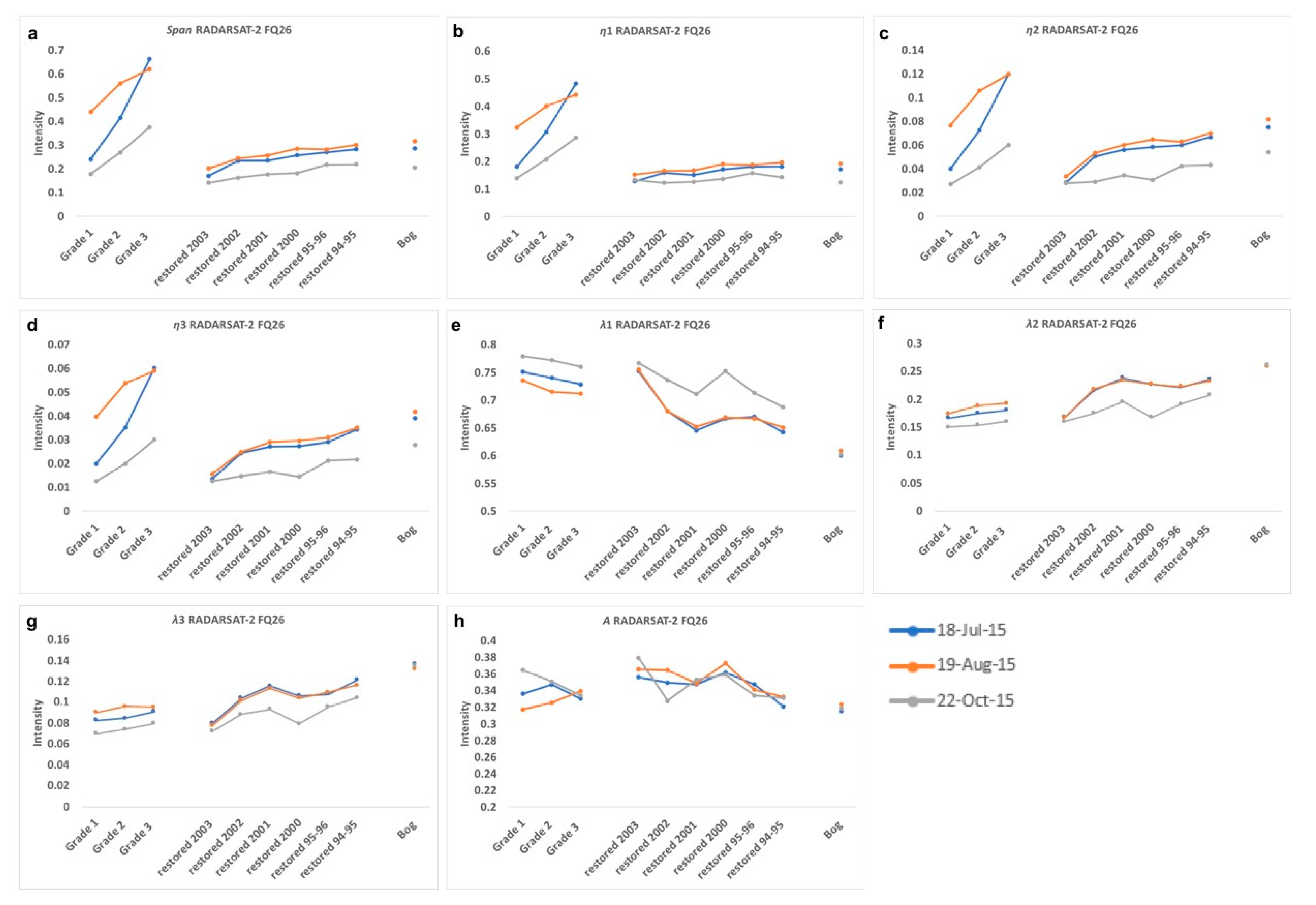
Figure 5.
Spectral signatures for natural shrub bog, restored peat, and actively harvested peat using the RADARSAT-2 FQ26 images. (a) Total power (span), (b) dominant eigenvalue, (c) secondary eigenvalue, (d) tertiary eigenvalue, (e) normalized dominant eigenvalue, (f) normalized secondary eigenvalue, (g) normalized tertiary eigenvalue, and (h) anisotropy.
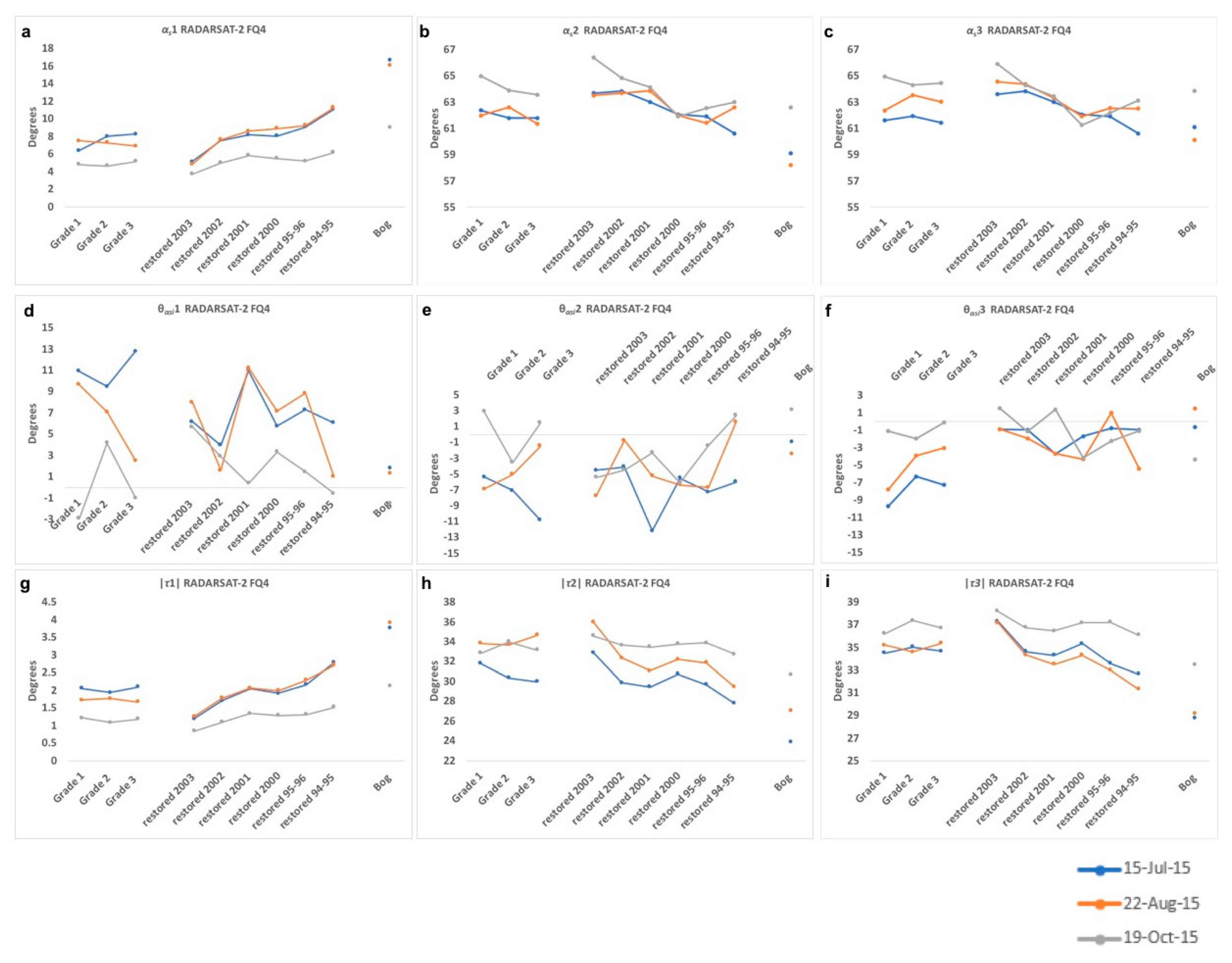
Figure 6.
Spectral signatures for natural shrub bog, harvested peat, and restored peat using RADARSAT-2 FQ4 imagery. (a–c) Dominant, secondary, and tertiary scattering-type magnitude, (d–f) dominant, secondary, and tertiary scattering-type phase, and (g–i) dominant, secondary, and tertiary absolute value of helicity, respectively.
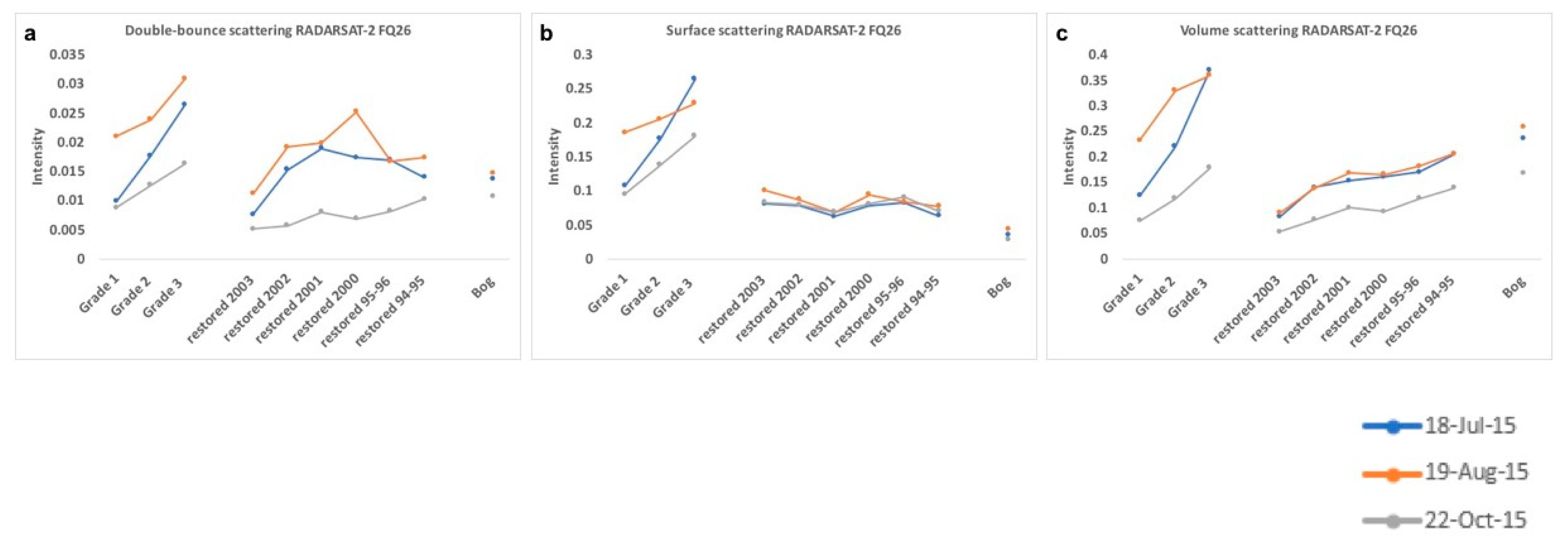
Figure 7.
Graphs show the spectral signatures of natural shrub bog, harvested peat, and restored peat when the Freeman–Durden decomposition was applied to RADARSAT-2 FQ26 images. Double-bounce scattering is presented in (a), surface scattering in (b), and volume scattering in (c). All values are represented in decibels (dB).
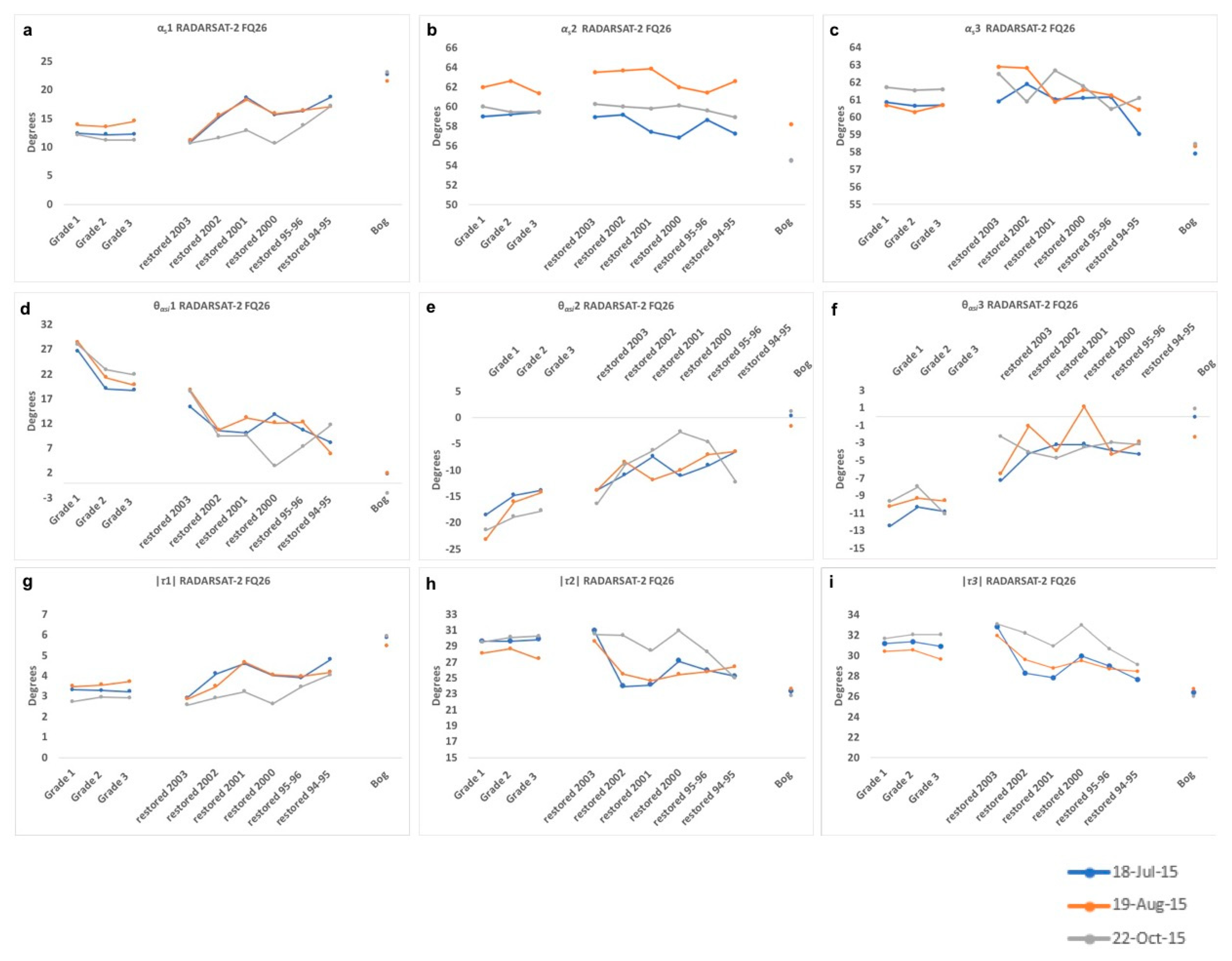
Figure 8.
Graphs show the spectral signatures for natural shrub bog, harvested peat, and restored peat derived from RADARSAT-2 FQ26 imagery. (a–c) Dominant, secondary, and tertiary scattering-type magnitude, (d–f) dominant, secondary, and tertiary scattering-type phase, and (g–i) dominant, secondary, and tertiary absolute value of helicity, respectively.
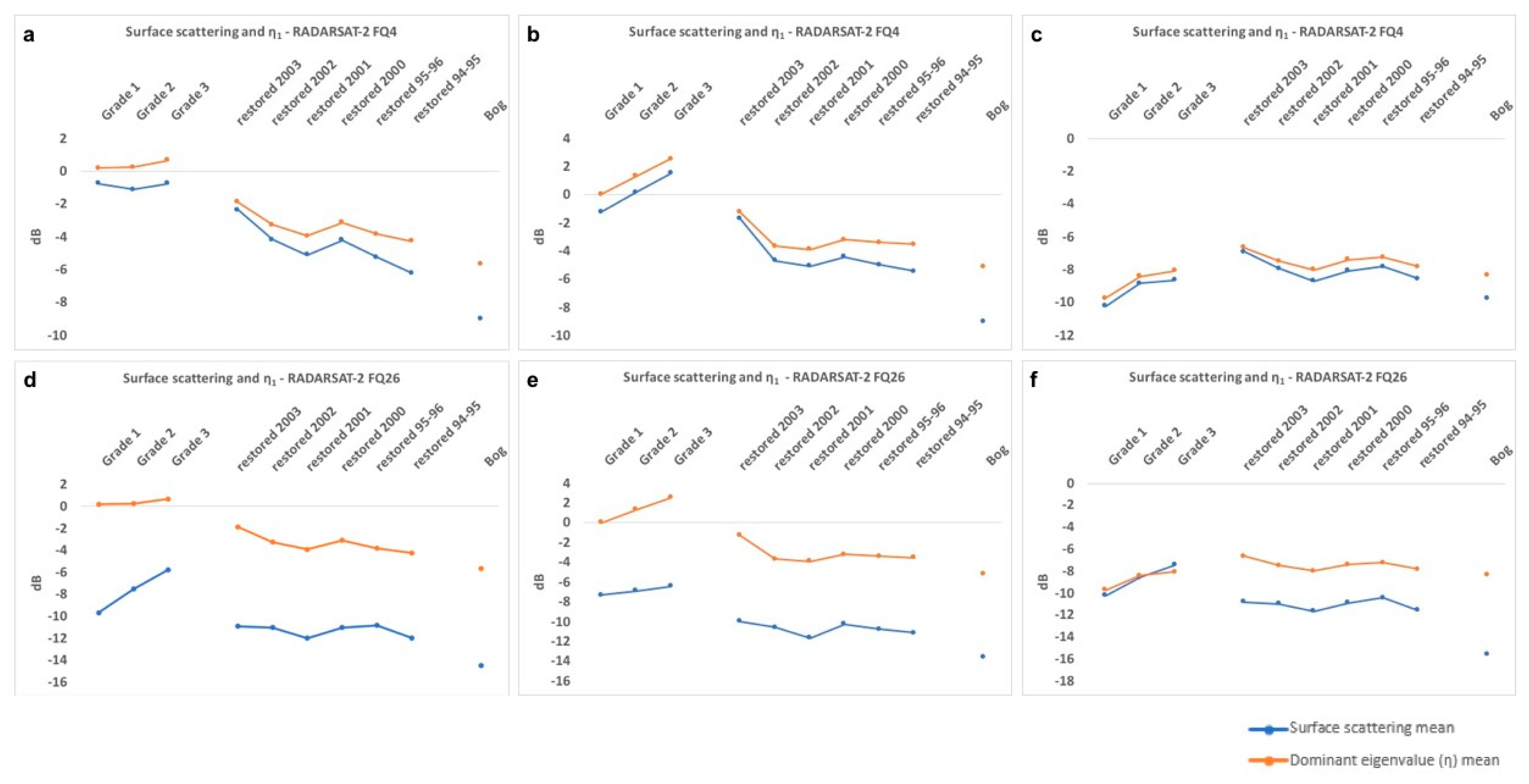
Figure 9.
Comparison of dB values from the FD rough surface scattering and the ICTD η1 for July 15 FQ4 (a), August 22 FQ4 (b), October 19 FQ4 (c), July 18 FQ26 (d), August 15 FQ26 (e), and October 22 FQ26 (f) 2015 RADARSAT-2 images.
Figure 9.
Comparison of dB values from the FD rough surface scattering and the ICTD η1 for July 15 FQ4 (a), August 22 FQ4 (b), October 19 FQ4 (c), July 18 FQ26 (d), August 15 FQ26 (e), and October 22 FQ26 (f) 2015 RADARSAT-2 images.
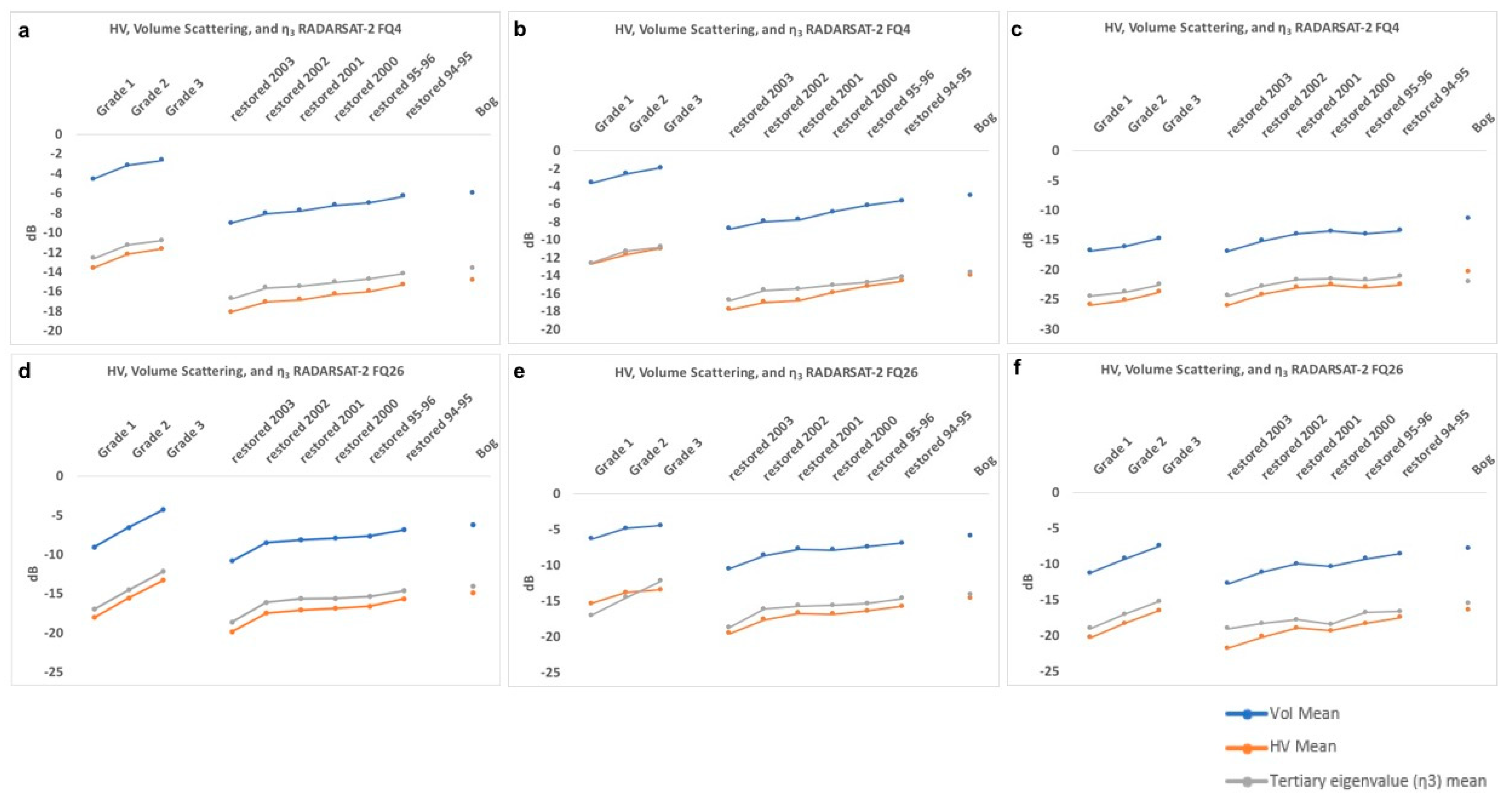
Figure 10.
Comparison of dB values from HV intensity, the FD volume scattering, and the ICTD η3 for July 15 FQ4 (a), August 22 FQ4 (b), October 19 FQ4 (c), July 18 FQ26 (d), August 15 FQ26 (e, October 22 FQ26 (f) 2015 RADARSAT-2 images.
Figure 10.
Comparison of dB values from HV intensity, the FD volume scattering, and the ICTD η3 for July 15 FQ4 (a), August 22 FQ4 (b), October 19 FQ4 (c), July 18 FQ26 (d), August 15 FQ26 (e, October 22 FQ26 (f) 2015 RADARSAT-2 images.
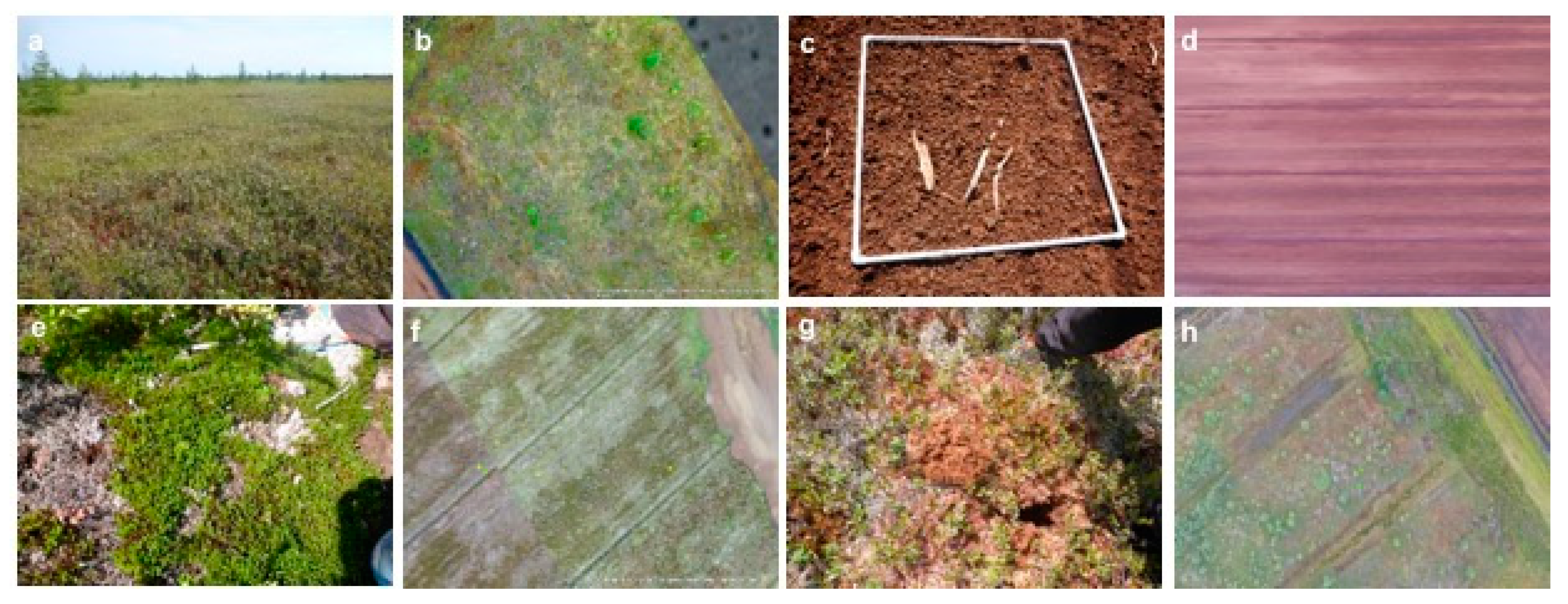
Figure 11.
Sainte-Marguerite-Marie peatland field site photos and UAS imagery. Photos (a) representative natural bog, (b) UAS imagery for the natural bog, (c) exposed peat layer prepared for harvest, (d) UAS imagery for harvest area, (e) post-restoration area with Polytrichum cover, (f) UAS imagery for Polytrichum covered area, (g) Predominantly Sphagnum moss-covered site, and (h) UAS imagery for a Sphagnum covered area.
Table 1.
Description of the RADARSAT-2 images used in this research.
Table 1.
Description of the RADARSAT-2 images used in this research.
| Beam Mode | Date | Nominal Resolution (m) | Nominal Incidence Angle (degrees) | Polarization |
|---|
| FQ4 | 15 July 2015 | 13.8–12.7 | 22.1–24.1 | HH+VV+HV+HV |
| FQ4 | 22 August 2015 | 13.8–12.7 | 22.1–24.1 | HH+VV+HV+HV |
| FQ4 | 19 October 2105 | 13.8–12.7 | 22.1–24.1 | HH+VV+HV+HV |
| FQ26 | 18 July 2015 | 7.4–7.3 | 44.4–45.7 | HH+VV+HV+HV |
| FQ26 | 19 August 2015 | 7.4–7.3 | 44.4–45.7 | HH+VV+HV+HV |
| FQ26 | 22 October 2015 | 7.4–7.3 | 44.4–45.7 | HH+VV+HV+HV |
Table 2.
Bhattacharya distance (BD) statistic for the FQ4 15 July 2015, and FQ26 18 July 2015, RADARSAT-2 images. The BD value indicates whether the spectral responses of natural shrub bog, restored peat, and actively harvested peat can be separated. Values range from 0 to 2.0. All values equal to or greater than 1.9 indicate good spectral separability.
| | Grade 1 | Grade 2 | Grade 3 | Restored 94–95 | Restored 95–96 | Restored 00 | Restored 01 | Restored 02 | Restored 03 |
|---|
| | FD | ICTD | FD | ICTD | FD | ICTD | FD | ICTD | FD | ICTD | FD | ICTD | FD | ICTD | FD | ICTD | FD | ICTD |
|---|
| RADARSAT-2 FQ4 BD 20150715 |
| Grade 2 | 0.3 | 0.5 | | | | | | | | | | | | | | | | |
| Grade 3 | 0.6 | 0.9 | 0.1 | 0.2 | | | | | | | | | | | | | | |
| Restored 94-95 | 1.1 | 1.5 | 1.2 | 1.4 | 1.5 | 1.7 | | | | | | | | | | | | |
| Restored 95-96 | 1.2 | 1.4 | 1.3 | 1.5 | 1.6 | 1.7 | 0.4 | 0.3 | | | | | | | | | | |
| Restored 00 | 1.3 | 1.6 | 1.5 | 1.7 | 1.7 | 1.9 | 0.6 | 0.6 | 0.1 | 0.3 | | | | | | | | |
| Restored 01 | 1.5 | 1.6 | 1.6 | 1.7 | 1.8 | 1.9 | 0.6 | 0.6 | 0.1 | 0.2 | 0.1 | 0.2 | | | | | | |
| Restored 02 | 1.5 | 1.6 | 1.6 | 1.7 | 1.8 | 1.9 | 0.9 | 0.7 | 0.3 | 0.3 | 0.1 | 0.2 | 0.1 | 0.2 | | | | |
| Restored 03 | 1.6 | 1.7 | 1.7 | 1.8 | 1.9 | 1.9 | 1.2 | 1.5 | 0.8 | 1.1 | 0.5 | 0.8 | 0.6 | 0.9 | 0.4 | 0.6 | | |
| Bog | 1.3 | 1.9 | 1.4 | 1.9 | 1.7 | 1.9 | 0.2 | 0.5 | 0.9 | 1.0 | 1.0 | 1.3 | 1.1 | 1.3 | 1.3 | 1.4 | 1.5 | 1.9 |
| RADARSAT-2 FQ26 BD 20150718 |
| Grade 2 | 0.6 | 0.8 | | | | | | | | | | | | | | | | |
| Grade 3 | 1.8 | 2.0 | 0.6 | 0.8 | | | | | | | | | | | | | | |
| Restored 94-95 | 0.6 | 1.1 | 0.1 | 0.7 | 0.9 | 1.6 | | | | | | | | | | | | |
| Restored 95-96 | 0.3 | 0.8 | 0.1 | 0.6 | 1.2 | 1.6 | 0.1 | 0.2 | | | | | | | | | | |
| Restored 00 | 0.3 | 0.7 | 0.3 | 0.7 | 1.4 | 1.9 | 0.2 | 0.3 | 0.0 | 0.1 | | | | | | | | |
| Restored 01 | 0.2 | 0.9 | 0.3 | 1.0 | 1.5 | 1.9 | 0.2 | 0.3 | 0.0 | 0.2 | 0.0 | 0.2 | | | | | | |
| Restored 02 | 0.1 | 0.5 | 0.3 | 0.7 | 1.5 | 1.8 | 0.3 | 0.4 | 0.1 | 0.1 | 0.1 | 0.2 | 0.0 | 0.2 | | | | |
| Restored 03 | 0.5 | 0.7 | 1.1 | 1.3 | 1.9 | 2.0 | 1.2 | 1.5 | 0.9 | 1.3 | 1.1 | 1.4 | 1.0 | 1.4 | 0.7 | 0.9 | | |
| Bog | 1.1 | 1.6 | 0.3 | 1.2 | 0.8 | 1.7 | 0.1 | 0.2 | 0.4 | 0.6 | 0.5 | 0.7 | 0.6 | 0.6 | 0.7 | 0.9 | 1.6 | 1.8 |
Table 3.
Values represent the Bhattacharya distance (BD) statistic for the RADARSAT-2 FQ4 22 August 2015, and FQ26 19 August 2015 images. This metric was used to determine whether the spectral responses of natural shrub bog, restored peat, and actively harvested peat can be separated. Values equal to or greater than 1.9 indicate good spectral separability and values below 1.9 indicate poor separability.
| | Grade 1 | Grade 2 | Grade 3 | Restored 94–95 | Restored 95–96 | Restored 00 | Restored 01 | Restored 02 | Restored 03 |
|---|
| | FD | ICTD | FD | ICTD | FD | ICTD | FD | ICTD | FD | ICTD | FD | ICTD | FD | ICTD | FD | ICTD | FD | ICTD |
|---|
| RADARSAT-2 FQ4 BD 20150822 |
| Grade 2 | 0.4 | 0.5 | | | | | | | | | | | | | | | | |
| Grade 3 | 0.8 | 1.1 | 0.4 | 0.6 | | | | | | | | | | | | | | |
| Restored 94-95 | 1.1 | 1.2 | 1.0 | 1.4 | 1.5 | 1.8 | | | | | | | | | | | | |
| Restored 95-96 | 1.1 | 1.2 | 1.0 | 1.4 | 1.6 | 1.8 | 0.4 | 0.2 | | | | | | | | | | |
| Restored 00 | 1.4 | 1.6 | 1.2 | 1.5 | 1.8 | 2.0 | 0.4 | 0.5 | 0.1 | 0.2 | | | | | | | | |
| Restored 01 | 1.5 | 1.7 | 1.3 | 1.6 | 1.9 | 2.0 | 0.7 | 0.6 | 0.2 | 0.3 | 0.1 | 0.3 | | | | | | |
| Restored 02 | 1.6 | 1.7 | 1.4 | 1.6 | 1.9 | 2.0 | 0.9 | 0.7 | 0.4 | 0.4 | 0.3 | 0.2 | 0.1 | 0.1 | | | | |
| Restored 03 | 1.6 | 1.7 | 1.2 | 1.4 | 1.9 | 1.9 | 1.2 | 1.5 | 0.9 | 1.3 | 0.7 | 1.0 | 0.6 | 1.0 | 0.6 | 0.8 | | |
| Bog | 1.3 | 1.8 | 1.3 | 1.9 | 1.7 | 2.0 | 0.3 | 0.6 | 0.8 | 1.0 | 0.9 | 1.2 | 1.2 | 1.3 | 1.4 | 1.4 | 1.6 | 1.9 |
| RADARSAT-2 FQ26 BD 20150819 |
| Grade 2 | 0.4 | 0.5 | | | | | | | | | | | | | | | | |
| Grade 3 | 0.6 | 0.8 | 0.2 | 0.3 | | | | | | | | | | | | | | |
| Restored 94–95 | 0.7 | 0.8 | 0.6 | 0.8 | 1.0 | 1.3 | | | | | | | | | | | | |
| Restored 95–96 | 0.6 | 0.8 | 0.6 | 0.9 | 1.1 | 1.5 | 0.1 | 0.1 | | | | | | | | | | |
| Restored 00 | 0.7 | 0.9 | 0.7 | 1.0 | 1.3 | 1.6 | 0.2 | 0.2 | 0.1 | 0.1 | | | | | | | | |
| Restored 01 | 0.8 | 1.1 | 0.8 | 1.1 | 1.4 | 1.7 | 0.1 | 0.2 | 0.0 | 0.1 | 0.1 | 0.2 | | | | | | |
| Restored 02 | 1.0 | 1.3 | 0.9 | 1.1 | 1.5 | 1.8 | 0.4 | 0.3 | 0.2 | 0.2 | 0.1 | 0.2 | 0.2 | 0.2 | | | | |
| Restored 03 | 1.6 | 1.8 | 1.4 | 1.5 | 1.9 | 2.0 | 1.3 | 1.3 | 1.1 | 1.2 | 1.1 | 1.2 | 1.1 | 1.2 | 0.6 | 0.8 | | |
| Bog | 0.8 | 1.0 | 0.8 | 1.1 | 1.0 | 1.3 | 0.2 | 0.2 | 0.5 | 0.4 | 0.7 | 0.6 | 0.6 | 0.5 | 1.1 | 0.9 | 1.8 | 1.8 |
Table 4.
Results of the Bhattacharya distance (BD) statistic comparing the separability of the spectral responses for natural shrub bog, restored peat, and actively harvested using the RADARSAT-2 FQ4 19 October 2015, and FQ26 22 October 2015 images. All values equal to or greater than 1.9 suggest good spectral separability and values below 1.9 suggest poor separability.
| | Grade 1 | Grade 2 | Grade 3 | Restored 94–95 | Restored 95–96 | Restored 00 | Restored 01 | Restored 02 | Restored 03 |
|---|
| | FD | ICTD | FD | ICTD | FD | ICTD | FD | ICTD | FD | ICTD | FD | ICTD | FD | ICTD | FD | ICTD | FD | ICTD |
|---|
| RADARSAT-2 FQ4 BD 20151019 |
| Grade 2 | 0.2 | 0.3 | | | | | | | | | | | | | | | | |
| Grade 3 | 0.7 | 0.9 | 0.3 | 0.4 | | | | | | | | | | | | | | |
| Restored 94–95 | 1.3 | 1.4 | 0.8 | 0.9 | 0.3 | 0.4 | | | | | | | | | | | | |
| Restored 95–96 | 1.0 | 1.1 | 0.5 | 0.6 | 0.1 | 0.2 | 0.1 | 0.2 | | | | | | | | | | |
| Restored 00 | 1.2 | 1.3 | 0.6 | 0.7 | 0.2 | 0.3 | 0.1 | 0.2 | 0.1 | 0.1 | | | | | | | | |
| Restored 01 | 1.1 | 1.3 | 0.5 | 0.7 | 0.1 | 0.2 | 0.2 | 0.2 | 0.1 | 0.2 | 0.1 | 0.2 | | | | | | |
| Restored 02 | 0.7 | 0.8 | 0.2 | 0.2 | 0.1 | 0.2 | 0.5 | 0.6 | 0.2 | 0.2 | 0.3 | 0.4 | 0.2 | 0.3 | | | | |
| Restored 03 | 0.8 | 1.0 | 0.4 | 0.4 | 0.8 | 0.8 | 1.2 | 1.3 | 0.9 | 1.0 | 1.0 | 1.1 | 0.9 | 1.1 | 0.5 | 0.5 | | |
| Bog | 1.8 | 1.9 | 1.5 | 1.7 | 1.2 | 1.3 | 0.5 | 0.7 | 0.8 | 1.1 | 0.7 | 0.9 | 0.8 | 0.9 | 1.2 | 1.4 | 1.7 | 1.8 |
| RADARSAT-2 FQ26 BD 20151022 |
| Grade 2 | 0.4 | 0.6 | | | | | | | | | | | | | | | | |
| Grade 3 | 1.5 | 1.8 | 0.5 | 0.6 | | | | | | | | | | | | | | |
| Restored 94–95 | 1.1 | 0.9 | 0.7 | 0.6 | 0.9 | 1.1 | | | | | | | | | | | | |
| Restored 95–96 | 0.6 | 0.9 | 0.2 | 0.4 | 0.7 | 0.9 | 0.3 | 0.2 | | | | | | | | | | |
| Restored 00 | 0.3 | 0.3 | 0.4 | 0.5 | 1.3 | 1.5 | 0.5 | 0.6 | 0.2 | 0.5 | | | | | | | | |
| Restored 01 | 0.5 | 0.5 | 0.5 | 0.5 | 1.2 | 1.4 | 0.3 | 0.3 | 0.1 | 0.3 | 0.1 | 0.2 | | | | | | |
| Restored 02 | 0.2 | 0.4 | 0.5 | 0.6 | 1.4 | 1.5 | 0.8 | 0.5 | 0.4 | 0.5 | 0.2 | 0.1 | 0.3 | 0.1 | | | | |
| Restored 03 | 0.4 | 0.4 | 1.0 | 0.5 | 1.8 | 1.4 | 1.4 | 0.7 | 1.1 | 0.7 | 0.8 | 0.2 | 1.0 | 0.3 | 0.3 | 0.2 | | |
| Bog | 1.6 | 1.7 | 1.2 | 1.4 | 1.2 | 1.6 | 0.3 | 0.6 | 0.9 | 0.8 | 1.2 | 1.4 | 0.9 | 1.0 | 1.4 | 1.2 | 1.8 | 1.5 |
Table 5.
The total power contributions from the Freeman–Durden decomposition. DB represents the percent of total power resulting from double-bounce backscatter, vol. the percent of total power from volume backscatter, and surf. the percent of total power from surface backscatter.
Table 5.
The total power contributions from the Freeman–Durden decomposition. DB represents the percent of total power resulting from double-bounce backscatter, vol. the percent of total power from volume backscatter, and surf. the percent of total power from surface backscatter.
| Peat State | % Total Power 15 July 2015 | % Total Power 22 August 2015 | % Total Power 19 October 2015 |
|---|
| | % DB | % Vol. | % Surf. | % DB | % Vol. | % Surf. | % DB | % Vol. | % Surf. |
|---|
| RADARSAT-2 FQ4 |
| Grade 1 | 2 | 29 | 70 | 2 | 36 | 62 | 2 | 18 | 81 |
| Grade 2 | 2 | 38 | 60 | 2 | 34 | 64 | 2 | 16 | 83 |
| Grade 3 | 2 | 39 | 60 | 2 | 31 | 67 | 2 | 19 | 79 |
| Restored 2003 | 2 | 17 | 81 | 2 | 16 | 82 | 2 | 9 | 90 |
| Restored 2002 | 3 | 28 | 69 | 3 | 31 | 66 | 2 | 16 | 83 |
| Restored 2001 | 3 | 34 | 63 | 3 | 34 | 63 | 2 | 22 | 76 |
| Restored 2000 | 3 | 32 | 65 | 3 | 35 | 62 | 1 | 22 | 77 |
| Restored 1995–1996 | 3 | 39 | 58 | 3 | 42 | 55 | 1 | 19 | 79 |
| Restored 1994–1995 | 4 | 48 | 49 | 3 | 48 | 49 | 2 | 24 | 74 |
| Natural shrub bog | 5 | 63 | 31 | 4 | 69 | 27 | 3 | 40 | 57 |
| RADARSAT-2 FQ26 |
| Grade 1 | 4 | 51 | 44 | 5 | 53 | 42 | 5 | 42 | 53 |
| Grade 2 | 4 | 53 | 43 | 4 | 59 | 37 | 5 | 44 | 51 |
| Grade 3 | 4 | 56 | 40 | 5 | 58 | 37 | 4 | 48 | 48 |
| Restored 2003 | 4 | 48 | 47 | 6 | 45 | 50 | 4 | 38 | 59 |
| Restored 2002 | 7 | 60 | 34 | 8 | 56 | 36 | 4 | 47 | 49 |
| Restored 2001 | 8 | 65 | 27 | 8 | 66 | 27 | 5 | 57 | 39 |
| Restored 2000 | 7 | 63 | 31 | 9 | 58 | 33 | 4 | 51 | 45 |
| Restored 1995–1996 | 6 | 63 | 30 | 6 | 64 | 30 | 4 | 54 | 42 |
| Restored 1994–1995 | 5 | 73 | 22 | 6 | 69 | 26 | 5 | 63 | 32 |
| Natural shrub bog | 5 | 83 | 12 | 5 | 82 | 14 | 6 | 81 | 13 |
Table 6.
Total power contributions from the three types of scattering mechanisms in the Touzi incoherent target decomposition (ICTD). λ1 is representative of the percentage of total power from rough surface backscattering, λ2 from double-bounce backscattering, and λ3 from volume backscattering.
Table 6.
Total power contributions from the three types of scattering mechanisms in the Touzi incoherent target decomposition (ICTD). λ1 is representative of the percentage of total power from rough surface backscattering, λ2 from double-bounce backscattering, and λ3 from volume backscattering.
| Peat State | % Total Power 15 July 2015 | % Total Power 22 August 2015 | % Total Power 19 October 2015 |
| | % λ1 | % λ2 | % λ3 | % λ1 | % λ2 | % λ3 | % λ1 | % λ2 | % λ3 |
| RADARSAT-2 FQ4 |
| Grade 1 | 86 | 9 | 5 | 83 | 11 | 6 | 90 | 6 | 3 |
| Grade 2 | 82 | 12 | 6 | 84 | 11 | 5 | 92 | 6 | 3 |
| Grade 3 | 82 | 12 | 6 | 85 | 10 | 5 | 90 | 7 | 3 |
| Restored 2003 | 91 | 6 | 3 | 91 | 6 | 3 | 95 | 4 | 2 |
| Restored 2002 | 84 | 11 | 5 | 83 | 12 | 5 | 92 | 6 | 3 |
| Restored 2001 | 82 | 12 | 6 | 82 | 12 | 6 | 88 | 8 | 4 |
| Restored 2000 | 83 | 11 | 5 | 82 | 12 | 6 | 89 | 7 | 3 |
| Restored 1995–1996 | 80 | 14 | 6 | 79 | 14 | 7 | 90 | 6 | 3 |
| Restored 1994–1995 | 76 | 16 | 8 | 77 | 16 | 8 | 88 | 8 | 4 |
| Natural shrub bog | 68 | 22 | 11 | 67 | 22 | 11 | 88 | 8 | 4 |
| | % Total Power 18 July 2015 | % Total Power 19 August 2015 | % Total Power 22 October 2015 |
| | % λ1 | % λ2 | % λ3 | % λ1 | % λ2 | % λ3 | % λ1 | % λ2 | % λ3 |
| RADARSAT-2 FQ26 |
| Grade 1 | 75 | 17 | 8 | 74 | 17 | 9 | 78 | 15 | 7 |
| Grade 2 | 74 | 17 | 8 | 71 | 19 | 10 | 77 | 15 | 7 |
| Grade 3 | 73 | 18 | 9 | 71 | 19 | 10 | 76 | 16 | 8 |
| Restored 2003 | 75 | 17 | 8 | 76 | 17 | 8 | 94 | 20 | 9 |
| Restored 2002 | 68 | 22 | 10 | 68 | 22 | 10 | 75 | 18 | 9 |
| Restored 2001 | 65 | 24 | 12 | 65 | 23 | 11 | 71 | 20 | 9 |
| Restored 2000 | 67 | 23 | 11 | 67 | 23 | 10 | 75 | 17 | 8 |
| Restored 1995–1996 | 67 | 22 | 11 | 67 | 22 | 11 | 73 | 20 | 10 |
| Restored 1994–1995 | 64 | 24 | 12 | 65 | 23 | 12 | 65 | 20 | 10 |
| Natural shrub bog | 60 | 26 | 14 | 61 | 26 | 13 | 60 | 26 | 14 |


