Article

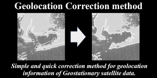
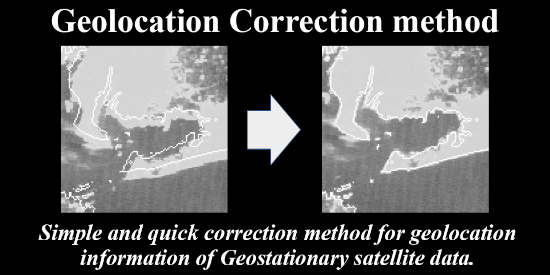
Geolocation Correction for Geostationary Satellite Observations by a Phase-Only Correlation Method Using a Visible Channel

1
Center for Environmental Remote Sensing (CEReS), Chiba University, 1-33 Yayoi-cho, Inage-ku, Chiba 263-8522, Japan
2
Weathernews Inc. (WNI), Makuhari Techno Garden, Nakase 1-3 Mihama-ku, Chiba-shi, Chiba 261-0023, Japan
3
National Institute for Environmental Studies (NIES), 16-2 Onogawa, Tsukuba City, Ibaraki 305-8506, Japan
*
Author to whom correspondence should be addressed.
Remote Sens. 2020, 12(15), 2472; https://0-doi-org.brum.beds.ac.uk/10.3390/rs12152472
Submission received: 30 June 2020 / Revised: 28 July 2020 / Accepted: 29 July 2020 / Published: 1 August 2020
(This article belongs to the Special Issue Earth Monitoring from A New Generation of Geostationary Satellites)

Abstract

:
This study describes a high-speed correction method for geolocation information of geostationary satellite data for accurate physical analysis. Geostationary satellite observations with high temporal resolution provide instantaneous analysis and prompt reports. We have previously reported the quasi real-time analysis of solar radiation at the surface and top of the atmosphere using geostationary satellite data. Estimating atmospheric parameters and surface albedo requires accurate geolocation information to estimate the solar radiation accurately. The physical analysis algorithm for Earth observations is verified by the ground truth. In particular, downward solar radiation at the surface is validated by pyranometers installed at ground observation sites. The ground truth requires that the satellite observation data pixels be accurately linked to the location of the observation equipment on the ground. Thus, inaccurate geolocation information disrupts verification and causes complex problems. It is difficult to determine whether error in the validation of physical quantities arises from the estimation algorithm, satellite sensor calibration, or a geolocation problem. Geolocation error hinders the development of accurate analysis algorithms; therefore, accurate observational information with geolocation information based on latitude and longitude is crucial in atmosphere and land target analysis. This method provides the basic data underlying physical analysis, parallax correction, etc. Because the processing speed is important in geolocation correction, we used the phase-only correlation (POC) method, which is fast and maintains the accuracy of geolocation information in geostationary satellite observation data. Furthermore, two-dimensional fast Fourier transform allowed the accurate correction of multiple target points, which improved the overall accuracy. The reference dataset was created using NASA’s Shuttle Radar Topography Mission 1-s mesh data. We used HIMAWARI-8/Advanced HIMAWARI Imager data to demonstrate our method, with 22,709 target points for every 10-min observation and 5826 points for every 2.5 min observation. Despite the presence of disturbances, the POC method maintained its accuracy. Column offset and line offset statistics showed stability and characteristic error trends in the raw HIMAWARI standard data. Our method was sufficiently fast to apply to quasi real-time analysis of solar radiation every 10 and 2.5 min. Although HIMAWARI-8 is used as an example here, our method is applicable to all geostationary satellites. The corrected HIMAWARI 16 channel gridded dataset is available from the open database of the Center for Environmental Remote Sensing (CEReS), Chiba University, Japan. The total download count was 50,352,443 on 8 July 2020. Our method has already been applied to NASA GeoNEX geostationary satellite products.

Graphical Abstract

1. Introduction

Clouds influence the Earth’s climate by cooling via reflecting solar radiation and by retaining heat via the absorption and emission of terrestrial radiation [1,2]. In addition, clouds are important in the energy balance of the Earth’s surface and top of the atmosphere and have complex relationships with the Earth system and feedback processes [3,4,5]. A deeper understanding of these feedback processes is needed for better understanding climate [6]. NASA’s CloudSat combined with other A-Train satellites produces a unique global view of the vertical structure of clouds and precipitation [7,8,9]. These data have provided new cloud physics and have changed our understanding of warm cloud with precipitation, demonstrating the effectiveness of the observation-based approach. Geostationary satellite observations are useful for studying clouds and radiation by using high-temporal-resolution, wide-area observations that can detect high-frequency changes, such as cloud stage changes, and these observations provide an archive of the history of Earth’s changes. In 2007, we started quasi real-time analysis of solar radiation at the surface and top of the atmosphere using the geostationary satellite HIMAWARI [10]. Our system shares the solar radiation and atmospheric parameters dataset with the research community by making the analysis results available promptly after the geostationary satellite observation. Our dataset “AMATERASS” was downloaded 73,674,172 times from 2013 to 8 July 2020 (http://www.cr.chiba-u.jp/databases/ftp-servers-weekly-access-logs.html). Currently, high-speed analysis provides a 10-min full-disk and 2.5-min Japanese regional solar radiation dataset based on high-temporal-resolution observations from the third-generation HIMAWARI satellite.
Several collaborative studies have highlighted the need to improve the accuracy of solar radiation analysis. Accurate analysis of the energy balance of the ground surface is a particularly important challenge. Land surface model simulations have been improved by high-temporal-resolution solar radiation at the surface [11]. Satellite surface downwelling solar radiation data were used for 1 × 1 km estimations of latent and sensible heat in surface processes and the surface radiation balance of the land surface model was improved by the geostationary satellite data. Furthermore, Wasa et al. investigated cooperative energy network formation in distributed autonomous microgrids by horizon control and game theory cooperative control [12]. Our satellite-derived surface downwelling solar radiation data were effective for optimizing the electric power grid. Kawano et al. proposed a voltage control method to prevent problems caused by distributed photovoltaic (PV) generator systems in electric power network service restoration [13]. They found that the satellite-derived 1 × 1 km high-temporal-resolution solar power data mitigated voltage deviation in the power grid. Watanabe et al. used satellite-derived solar radiation in a day-ahead scheduling method using machine learning for renewables [14]. These studies have found that more accurate surface downwelling solar radiation data are required. Damiani et al. validated the satellite-derived surface downwelling solar radiation data using ground base pyranometer observations [15]. The data showed a good correlation under clear sky conditions, but there were errors under cloudy conditions and large errors were seen with optically thin clouds and broken clouds, indicating the need for more research on clouds. We have found critical errors in cloud-radiation analysis with observed raw data. Figure 1 shows a typical example of a geolocation error in geostationary satellite observation data, in which accurate solar radiation and PV power at each point cannot be obtained.
HIMAWARI-1 to -5 are spin-stabilized satellites, and the error is periodic, whereas HIMAWARI-6 to -9 are three-axis-stabilized satellites, and thus errors occur randomly and may be caused by changes in the time-dependent satellite attitude and orbit position. High-temporal-resolution geostationary satellite data are useful for studying cloud generation and time-dependent changes in clouds, providing temporal and spatial information over a wide area; therefore, geolocation accuracy is critical. Validation of this data with ground observations is difficult. For example, to perform parallax correction based on cloud height, each pixel must first be linked accurately to latitude and longitude. Therefore, we initially focused on building quality data materials for estimating solar radiation. Atmospheric parameters are retrieved using instantaneous geostationary satellite observation data based on surface albedo, which is estimated from the instantaneous observation statistics. Atmospheric parameters and surface albedo require accurate geolocation information to provide accurate physical quantities. Similarly, the ground truth requires that the satellite observation data pixels be accurately linked to the location of the observation equipment on the ground. Thus, geolocation error hinders the development of accurate analysis algorithms, and accurate observational information with geolocation information based on latitude and longitude is a fundamental requirement.
Geostationary satellites use star sensors to determine attitude accurately [16]. Current star trackers with rate sensors provide accurate satellite navigation information about the satellite position and attitude within the orbit. The satellite position is determined as a function of time (orbit) and orientation of the imager reference optical axis (roll, pitch, yaw) with respect to the reference orbital axis (attitude). The accuracy of the navigation information is the first element in the geolocation accuracy of the observed data. The correction of the geolocation information is aided by landmark analysis through the cross-correlation method by using a template of several target points to obtain the correction value by image pattern matching registration [17]. Various satellite data registration techniques have been devised [18]. The wavelet method is applied to polar orbit satellites. The National Oceanic and Atmospheric Administration (NOAA) Advanced Very High Resolution Radiometer (AVHRR) and the Landsat Thematic Mapper (TM) use high-frequency wavelet feature registration [19]. This method is similar to edge-based correlation, but exploits the multiresolution nature of a wavelet decomposition. For geostationary satellites, Dan et al. proposed the slope-restricted multi-scale feature-matching algorithm [20]. The error was suppressed by narrowing the retrieval range from subsampled images registration of multi-scales. Hou et al. introduced multi-level grids for accurate registration [21]. Matching the coastline using grids of 12 scales reduced the effects of cloud contamination. However, high-speed accurate correction is required for high-temporal-resolution (10 and 2.5 min) and wide-area observations to analyze atmospheric and surface data correctly.
Herein, we introduce a high-speed, accurate correction method for geostationary satellite data using phase-only correlation (POC) processing with a visible channel [22,23,24]. The POC method provides a clear solution in a single calculation without iterative retrieval. Geostationary satellite data are equivalent to the Level-1A product because the pixels are not directly linked to latitude and longitude coordinates. Our method allows latitude and longitude information to be registered accurately. We obtain the Level-1B product using a high-speed calculation method for geostationary satellite observations. Although our method is applicable to all geostationary satellites, we use HIMAWARI-8 as an example in this study.

2. Third-Generation Geostationary Satellite HIMAWARI

In this section, the HIMAWARI-8/Advanced HIMAWARI Imager (AHI) configuration and HIMAWARI standard data are described. HIMAWARI-8/AHI was launched on 7 October 2014, and officially began operation on 7 July 2015. Its sensor has 16 channels from visible to infrared, with improved observation performance compared with the sensors up to HIMAWARI-7. Sensor radiometric calibration schemes have been proposed for the Global Space-Based Inter-Calibration System and World Meteorological Organization [25,26,27]. Therefore, we can analyze and discuss the physical quantities. The temporal resolution of observations has improved drastically, with high-temporal-resolution observations performed every 10 min in full-disk observations and every 2.5 min in the Japanese region. We discuss the 10-min full-disk observations as an example. Figure 2 shows the AHI full-disk scanning outlines. Each horizontal band represents a scanning swath and the scanning direction is west to east. A large area is scanned in each swath. The AHI consists of the following focal plane modules (FPMs): visible and near-infrared; midwave infrared; and longwave infrared [28]. Table 1 shows the channel wavelengths and spatial resolution for the FPMs. Channel 3 (0.64 μm) has a special spatial resolution of 0.5 × 0.5 km. Table 2 shows the specifications of the AHI channel detector elements. In the specifications, the rows are the number of cross-track direction detector arrays and the columns are the number of spare detectors. AHI has a redundant structure to ensure continuous, stable observations. The best detector for each row is selected during operation. Therefore, each FPM is a two-dimensional array internally and a line array externally. The instantaneous field of view of each channel is small for the spatial resolution and the sampling by the detector is dense. This shows that the raw sampling by each detector does not directly constitute a pixel. The actual pixels for each channel are resampled using a 4 × 4 kernel as follows (Figure 3).
P = i = 1 4 j = 1 4 w i w j S i , j i = 1 4 j = 1 4 w i w j
    x n + 1 x n = A S D    
    i w i = 1    
    j w j = 1    
where, P is a channel pixel value and ASD is the angular sample distance. The x series is the nominal position of sampling S and w is the weighting value based on ASD. Each pixel is converted to a normalized geostationary projection. The satellite is fixed in a virtual orbit, with the distance from the Earth’s center to the virtual satellite of 42,164 km (140.7° E at the equator). Simultaneously, registration is performed by landmark matching. These processes mean that the data user is not affected by problems such as slight changes in orbit and changes in the satellite attitude. Although geostationary satellites appear stationary in a virtual orbit, the actual accuracy is not sufficient. The 0.5 km resolution channel contains the most spatial information and it has a resolution better than 0.5 km before resampling. Therefore, it is the most suitable channel for geolocation information correction.

3. Geolocation Correction Method

Geostationary satellites observe Earth from geostationary orbit. Because the satellite is stationary with respect to Earth, high-temporal-resolution observations can be obtained from the same point, and thus high-speed, accurate geolocation correction is important. We applied the POC method using two-dimensional fast Fourier transform (FFT) to geostationary satellite observation data, based on the 1-s mesh data of the Shuttle Radar Topography Mission (SRTM) [29].

3.1. POC Method

We introduce the POC method and its application to correcting geolocation information. The two-dimensional FFT of f (x, y) is defined as
F ( u , v ) = f ( x , y ) e 2 π ( u x + v y ) i d x d y = F r ( u , v ) + i F i ( u , v )
where u and v are spatial frequencies. Two-dimensional data f (x, y) are transformed to F (u, v) as real F r and imaginary F i parts. When the satellite and the reference data are N × N, the FFT is
F ( u , v ) = 1 N x = 0 N 1 y = 0 N 1 f ( x , y ) e 2 π ( u x + v y ) i N
    G ( u , v ) = 1 N x = 0 N 1 y = 0 N 1 g ( x , y ) e 2 π ( u x + v y ) i N    
where f(x, y) and g(x, y) are satellite observations and references, respectively. The normalized mutual power spectrum R(u, v) is
R ( u , v ) = F ( u , v ) G ( u , v ) ¯ | F ( u , v ) G ( u , v ) ¯ |
where G ( u , v ) ¯ is the complex conjugate of G ( u , v ) . Because R(u, v) contains phase difference spectrum information, the phase difference correlation is obtained by the inverse Fourier transform of R(u, v).
r ( x , y ) = 1 N u = 0 N 1 v = 0 N 1 R ( u , v ) e 2 π ( u x + v y ) i N
The correlation value coordinates, r(x, y), represent the position error between the satellite and reference data. An FFT was used to reduce the computational cost of discrete Fourier transforms to 2 N 2 l o g 2 N / N 4 [30]. The Hamming window function was used to suppress the effect of high frequencies at the edges.
w ( x , y ) = 0.54 0.46 c o s 2 π ( x , y ) , ( 0 x 1 0 y 1 )
Generally, the cross-correlation method has an ambiguous trend when approaching the correct answer. The answer is sought by relying on the gradient from the correlation with the coordinates, depending on the pixel value and it is necessary to adjust the reference and observation brightness equally. The hill climbing method is effective when the gradient clearly shows an answer, although in most cases, the gradient is small and obtaining an exact answer requires many computational iterations. However, a steep gradient may hinder the search for the correct answer. This is a major issue for balancing computational cost and accuracy. Figure 4 shows an example of the calculation of the POC for r(x, y). The POC method calculates a clear correlation based on phase information rather than pixel value, and thus it is not necessary to adjust the brightness equally and the method is resistant to noise and changes in pixel value. In addition, because the answer can be obtained with a single calculation, iterative retrieval is not required, reducing the calculation cost, which is crucial in geolocation correction. High-speed calculations correspond to the high-temporal-resolution observation of geostationary satellites and can accept many target points, which allows highly accurate correction. The satellite observes the changes, and we analyze changes in aerosols, clouds, and ground cover. However, geolocation correction analyzes the unchanged signal; therefore, a method that is resistant to change is required.

3.2. Registration and Map Projection

This section describes the reference data and map projection. POC provides the correlation of the phase information of the satellite with the reference data. The optimal reference data are the registered satellite observation data, and accurately registered satellite data provide the best results. However, generating sufficient reference data for multiple target points manually is tedious and POC should be used for full automation. Because POC obtains the correlation of phase information, satellite and reference data do not necessarily have to look similar. In this study, we use the SRTM 1-s mesh data version 3 as reference, which are three-dimensional topographical data. The satellite visible channel sensor observes the reflectance of the Earth’s surface and the atmosphere overlap. The terrain does not change momentarily and it shares signal elements with geostationary satellite data. We used the coastline for reference because it provides the most visible landmark in the SRTM data. The coastline was created using not only elevation but also water and ocean mask (Figure 5) and was converted to a normalized geostationary projection for use as a reference in the disk image observed by the geostationary satellite [31]. The projection is defined as
( l o n l a t ) = f ( C L )
where C and L indicate the disk image position address of the column and line, respectively. This conversion provides the latitude and longitude at each point of the disk image are obtained. The link between latitude and longitude information and the disk image pixels converts SRTM data into a disk image. The following equations are used to obtain the specific point information corresponding to the disk image.
l o n = a r c t a n s 2 s 1 + l o n s b
    l a t = a r c t a n 1.006739501 s 3 s x y    
    s 2 = s n s i n ( C ) c o s ( L )    
    s 3 = s n s i n ( y )    
    s x y = s 1 2 + s 2 2    
    s n = h d s t c o s ( C ) c o s ( L ) s d c o s 2 ( L ) + 1.006739501 s i n 2 ( L )    
    s d = ( h d s t c o s ( C ) c o s ( L ) ) 2 1737122264 ( c o s 2 ( L ) + 1.006739501 s i n 2 ( L ) )    
where, h d s t is the distance between the center of the Earth and the satellite and l o n s b is a nominal satellite point. Geostationary satellite data are projected from the actual satellite position to a convenient position and l o n s b indicates the projected geostationary orbit position. Thus, h d s t = 42,164 km and l o n s b     = 140.7 E. Figure 6 shows the disk image based on SRTM data used as a reference for the converted coastline. The image resembles the virtual observation disk image derived from the topography data and accurately shows the coastline. Figure 7 shows the 22,709 POC target points picked around the coastline for every 10-min observation disk image. The target points used the disc image center as a reference center and are based on ±60°. However, the Intertropical Convergence Zone cloud often obscured the target. Therefore, the east-west direction, high-angle region was limited. A total of 125 × 125 pixels was cut out around each point, and the satellite data error was calculated by the POC method. However, the discontinuity of the edge caused a problem in the FFT. Equation (5) shows that the FFT was based on a signal of infinite length; thus, dummy data were added to reduce the non-alignment at the edge of the target window. The FFT had a target of N = 128 based on the FFT processing data, which had a power of two. POC is resistant to disturbance and is unaffected by small cloud contamination in the target window. Quality control eliminated much cloud contamination target when the coastline information was not available due to cloud. If the average reflectance of the target point 125 × 125 was over 0.2 or, when no clear correlation appeared, the point was rejected. Clouds along the coastline sometimes resulted in an unclear correlation. Thus, samples with r less than 15 were rejected. Outliers were excluded based on scanning swath statistics of the correction values for each target point. The standard deviation is quality controlled to be less than 0.5. The correction value was determined by each ±25 line average and summarized in 22,000 line with interpolation and extrapolation. The error corrections and links to the correct pixel point column and line are shown below.
( C L ) = f ( l a t l o n )
The transformation in Equation (19) is the inverse of Equation (11). Each observed pixel was registered to a latitude and longitude by map projection, and the data for each point were converted to the latitude and longitude gridded format from the observation disk, using the following formulas.
C = a r c t a n ( r 2 r 1 )
    L = a r c s i n ( r 3 r n )    
    r 1 = h d s t r 1 c o s ( c l a t ) c o s ( l o n l o n s b )    
    r 2 = r l c o s ( c l a t ) s i n ( l o n l o n s b )    
    r 3 = r l s i n ( c l a t )    
    r n = r 1 2 + r 2 2 + r 3 2    
    r l = E p o l 1 0.00669438444 c o s 2 ( c l a t )    
    c l a t = a r c t a n ( 0.993305616 t a n ( l a t ) )    
where, E p o l is the polar radius of Earth. The corresponding pixel positions were corrected by the column offset and line offset, COFF and LOFF, respectively, where COFF and LOFF are the calculated correction values modified by POC. Therefore, the target pixel was calculated as
C = C O F F + n i n t ( C 2 16 C F A C )
    L = L O F F + n i n t ( L 2 16 L F A C )    
where CFAC and LFAC are the column scale factor and line scale factor, respectively. The observed disk image does not contain latitude and longitude information; therefore, each pixel was converted into latitude and longitude using these processes. The COFF and LOFF of each channel were converted based on relative calibration to obtain all channels. Compensation on the highest-resolution channels provided better COFF and LOFF for all channels. Figure 8 shows the observation data in the latitude–longitude orthogonal coordinate system. The observation data can be converted into any coordinate system that is easy to use by linking the data with latitude and longitude information. The use of the observation information was limited to ±60° because the spatial resolution deteriorated in the outer circumference area of the disc. The gridded format geolocation accuracy was provided by the corrected COFF and LOFF. The registered satellite data were obtained by these processes. In the second step, new reference materials were obtained from the registered satellite data statistics. The coastline correction provided the initial correction data. Reference data from registered satellite data provided better results. However, the optimal statistics for the period require further discussion. This study focuses on the first step of SRTM data correction.

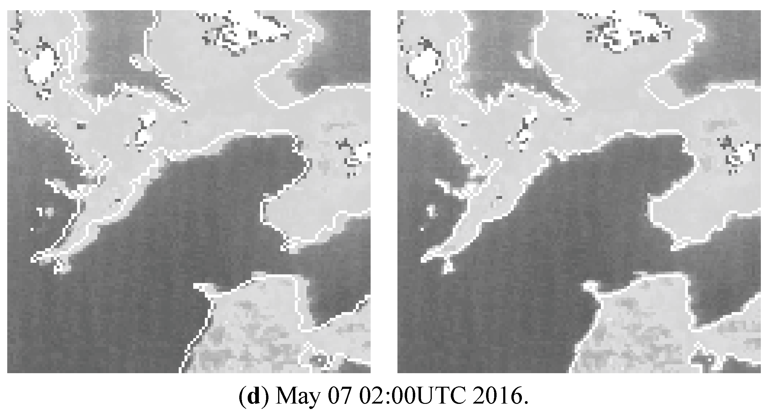
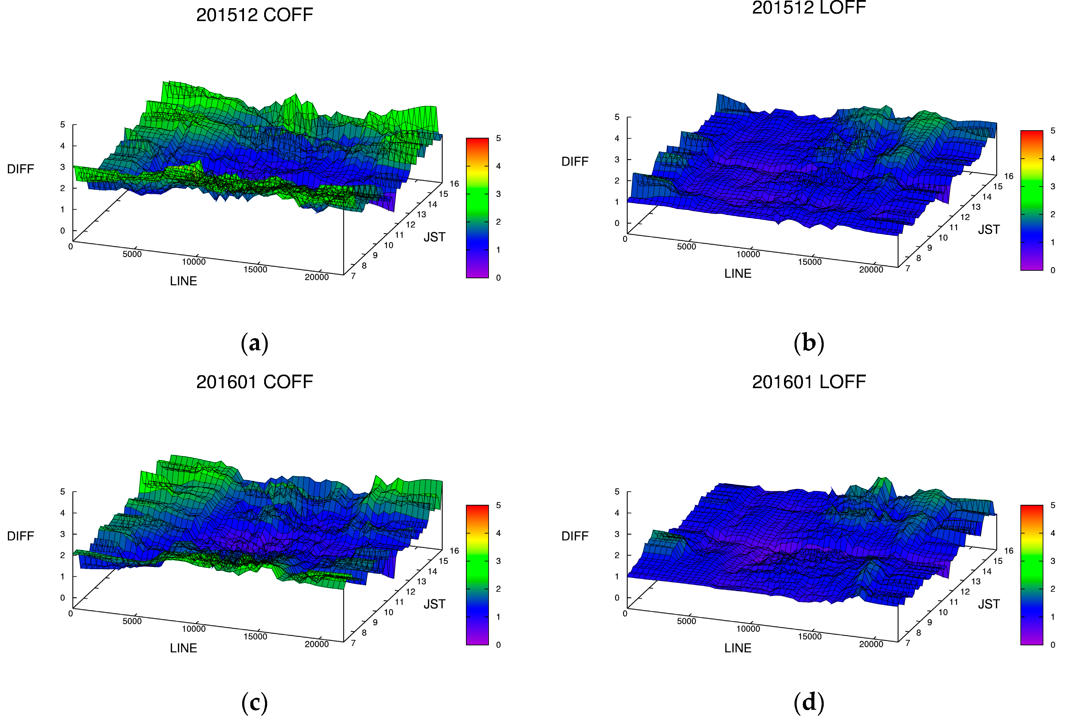
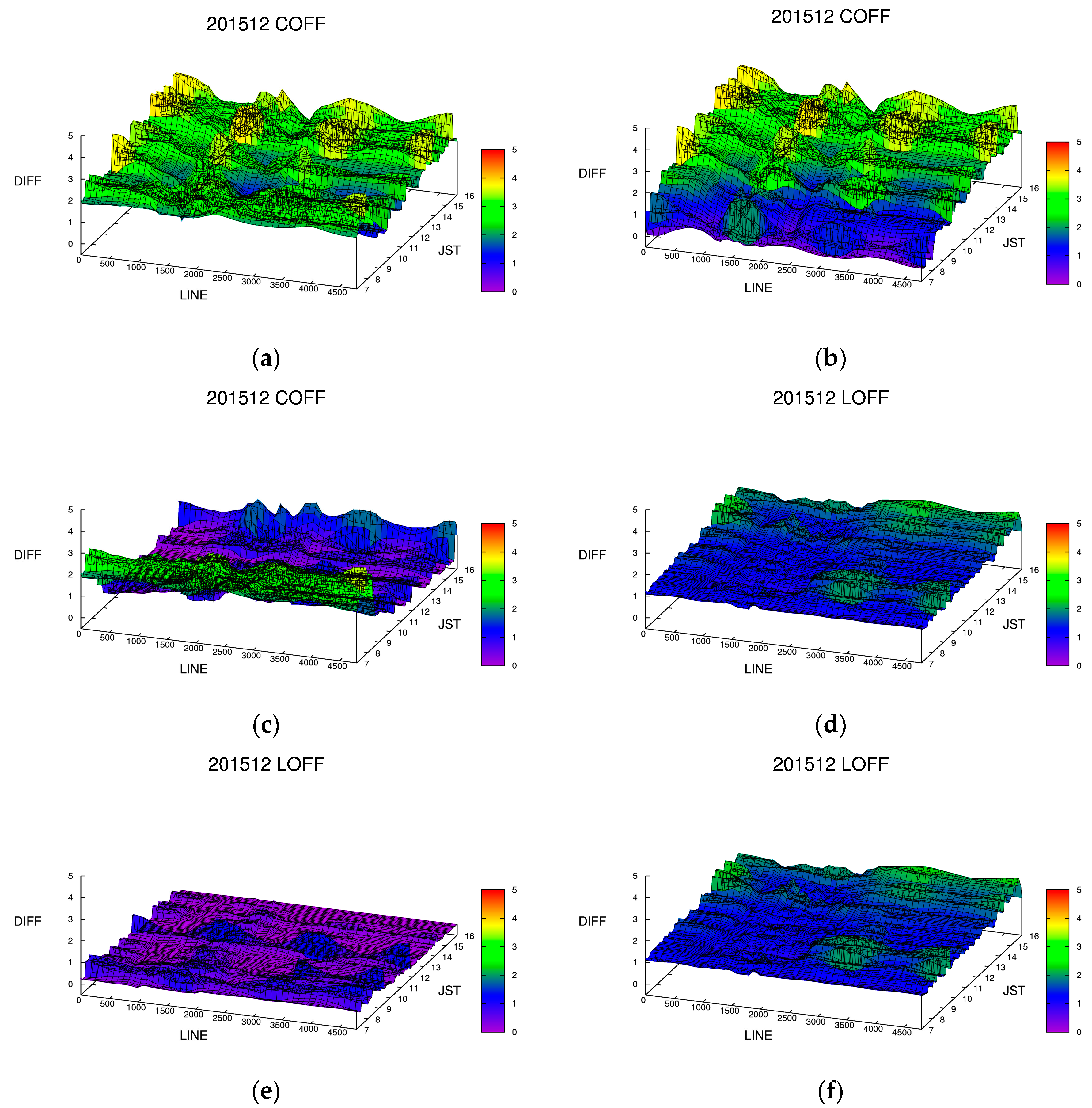
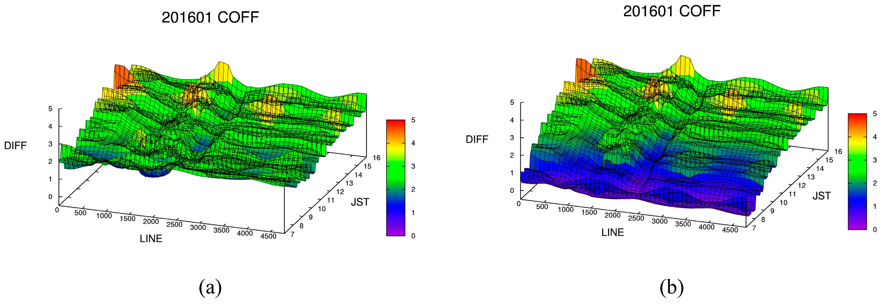
4. Results and Discussion

This section presents and discusses the correction results. The POC method provided high-speed correction by two-dimensional FFT and could accept multiple target points. Coastline data based on SRTM data were used as a reference for accuracy correction. Each target point process was executed by 88-thread parallel calculations, which took approximately 10 s. For the 10-min observations, 22,709 target points were used. This method provided superior performance for quasi real-time analysis by high-speed processing. Typical HIMAWARI-8 results are shown in Figure 9. Each point was randomly selected and clipped from the full-disk data. The images in the left column are raw data, and those in the right column are corrected data. Figure 9a is the Tokyo Bay area, Japan, which has a complex coastline. Corrections in complicated terrains were possible; however, misidentifications of small coastlines did not occur. Figure 9b shows a cloud-contaminated image sample from the west side of Australia, where there are clouds around the coastline. However, the despite the clouds, the correction method provided the exact position, which is crucial in geolocation correction for visible sensor data because most areas of Earth observation data include clouds. The point covered by much clouds was excluded in this method, but cloud inclusion could not be completely ruled out in many target areas. In addition to accuracy, the correction method must be resistant to external disturbances, such as clouds. Estimating solar radiation and PV power generation requires the exact location of clouds to be determined for each observation data point. Figure 9c shows the cloud-contaminated complex coastline of Mikawa Bay, Japan. The coastline was unclear and there was noise in the sea area. Multiple problem overlay is highly problematic in position analysis, with each factor decreasing the accuracy; however, the POC method obtained the correct position. Figure 9d shows the coastline changes due to clouds, with part of the sea looking like land. Disturbances that are indistinct, such as thin clouds, often resemble changes in terrain that can be difficult to distinguish visually without reference data. Because POC uses the correlation of phase information, partially uncorrelated areas are not a problem and partial topographic temporal changes do not affect correction accuracy. An example of the monthly statistics of COFF and LOFF error values obtained from the 10-min full-disk observations are shown in Figure 10. Figure 10a shows the column offset error. The difference between morning and evening tended to be large, but the accuracy remained stable during the day. However, in the early morning and at sunset, the visible sensor has a weak solar spectrum, making it difficult to distinguish noise from signal. This is not necessary near the polar region due to the absence of targets. The above trends were derived from extrapolation. However, the use of observation information is limited to 60°N–60°S, presenting no complications. The line offset error in Figure 10b is more stable compared with the column offset error. Polar axis stability indicated the accuracy of the star tracker and navigation information. In contrast, the east–west direction inaccuracies may be related to mirror swing sensor scanning and geostationary orbit stability with respect to the Earth, or processing of resampling and projection by navigation information. Higher accuracy was required for each pixel to be converted to a normalized geostationary projection. These trends remained consistent throughout the other periods (Figure 10c,d). The observations performed every 10 min were stable. Figure 11 shows the monthly maximum error value statistics of the COFF and LOFF for rapid scanning in the Japanese region for the 2.5-min observations, with larger values compared with the 10-min full-disk observations. For the 2.5-min observations, 5826 target points were used. Figure 11a shows the column offset error value, which is considerably higher than that in Figure 10a,c, reaching a value close to 4. The error value showed an unusual trend. Figure 11b,c show the east and west direction statistics, respectively. The error value tended to be large on the west side in the morning, whereas it tended to be significantly larger on the east side toward the evening, indicating that the raw data tended to drift from west to east over time. The eastern drift in the evening was much larger than the western drift in the morning. LOFF remained as stable as in the full-disk observations (Figure 11d). The stability of LOFF is a feature of HIMAWARI-8/AHI, regardless of the observation area. The drift to the north was small and the error was negligible (Figure 11e). The error in the north–south direction was a shift of about 1 pixel to the south (Figure 11f). These trends were similar in other periods (Figure 12), confirming the accuracy of the satellite’s navigational information provided by the star tracker. However, the increasing error in the east–west direction was unusual. We could not conclude whether these were JMA first-stage landmark matching errors due to disturbances like cloud contamination. Ground-based data processing may have been simplified because the observation data are released every 2.5 min, and it is possible that the first-stage landmark matching was not performed for all observation data. Careful confirmation of data is required to show the exact location of the cloud or land target every 2.5 min. At high speeds, our method can alleviate these errors. In addition, to understand the COFF and LOFF error values better, it must be noted that they indicate the error on the observation disk, which is the error in the nadir of the satellite. Geostationary satellites observe the Earth as a disk image. At the outer edge of the disc the spatial resolution deteriorates, as indicated by the area covered by 1 pixel in the disk image (Figure 13). Therefore, depending on the satellite viewing angle, the latitude–longitude gridded format can have a larger error than the COFF and LOFF error values. This problem is an important and basic issue for all geostationary satellites. Figure 14 shows the notable error around San Francisco Bay Area in GOES-16 observation. COFF and LOFF errors are only about 4 and 2. But big error has occurred in gridded format (error is about 5 km). The error disturbs the parallax correction and the physical analysis of atmosphere and land surface.

5. Conclusions

We developed a high-speed geolocation information correction method using POC. The positional information of observation data from geostationary satellites changes due to slight changes in attitude; however, observation data based on accurate positional information are a prerequisite for atmosphere and land target analyses. Our method provided fast, accurate corrections of the base data. The two-dimensional FFT process is fast and allows multiple correction targets in short time intervals. A target of 22,709 points was used for the 10-min full-disk observations and a target of 5826 points was used for the 2.5-min Japanese regional observations from HIMAWARI-8/AHI. The reference dataset was created based on the SRTM 1-s mesh data. Converting coastline information to a normalized geostationary projection is important for accurate correction. The POC method showed considerable resistance to disturbance and accurate correction was not hindered by cloud contamination over the correction target. The LOFF error value tended to give smaller errors than the COFF. The column and line offset statistics for periodic 10-min observations were stable. Additionally, the COFF and LOFF error values for the 2.5-min rapid observations gave a larger error than for the 10-min observations. Error statistics indicated that the error occurrence increased over time, which could be resolved by using our method. The method was sufficiently fast to be applied to quasi real-time analysis of solar radiation at the surface and top of the atmosphere. The corrected HIMAWARI 16 channel gridded dataset is already available from the Open Database of the Center for Environmental Remote Sensing (CEReS), Chiba University, Japan. The total download count was 50,352,443 on 8 July 2020 (http://www.cr.chiba-u.jp/databases/ftp-servers-weekly-access-logs.html). Although we used HIMAWARI-8/AHI as an example in this work, our method is applicable to all geostationary satellites. This method has already been applied to NASA GeoNEX geostationary satellite products.

Author Contributions

Conceptualization, H.T. and T.N.; methodology, H.T. and T.S.; software, H.T. and T.S.; formal analysis, H.T. and T.S.; investigation, H.T. and T.S.; resources, H.T. and A.H.; writing–original draft preparation, H.T.; writing—review and editing, A.H. and T.N.; visualization, H.T. and T.S.; supervision, A.H. and T.N.; project administration, A.H. and T.N.; funding acquisition, H.T., A.H., and T.N. All authors have read and agreed to the published version of the manuscript.

Funding

This study is partially supported by the Virtual Laboratory (VL) project, supported by the Ministry of Education, Culture, Sports, Science and Technology (MEXT), Japan, and JST/CREST: the JST/CREST/EMS fund, grant number JPMJCR15K4, Japan.

Acknowledgments

The author appreciates the useful comments and suggestions about HIMAWARI data processing by A. Okuyama and M. Takahashi. The real-time HIMAWARI data provided by Weathernews Inc. (WNI), D. Abe and Y. Seto. Special thanks are devoted to R. Nemani and researchers of NASA Earth Exchange (NEX) for collaborative research of geostationary satellites GOES. Also, there were many valuable comments and suggestions by the reviewers.

Conflicts of Interest

The authors declare no conflict of interest.

References

  1. Manabe, S.; Wetherald, R.T. Thermal equilibrium of the atmosphere with a given distribution of relative humidity. J. Atmos. Sci. 1967, 24, 241–259. [Google Scholar] [CrossRef] [Green Version]
  2. Schneider, S.H. Cloudiness as a global climate feedback mechanism: The effects on the radiation balance and surface temperature of variations in cloudiness. J. Atmos. Sci. 1972, 29, 1413–1422. [Google Scholar] [CrossRef] [Green Version]
  3. Tsushima, Y.; Manabe, S. Influence of cloud feedback on annual variation of global mean surface temperature. J. Geophys. Res. 2001, 106, 22635–22646. [Google Scholar] [CrossRef] [Green Version]
  4. Tsushima, Y.; Abe-Ouchi, A.; Manabe, S. Radiative damping of annual variation in globalmean surface temperature:comparison between observed and simulated feedback. Clim. Dyn. 2005, 24, 591–597. [Google Scholar] [CrossRef]
  5. Tsushima, Y.; Brient, F.; Klein, S.A.; Konsta, D.; Nam, C.C.; Qu, X.; Williams, K.D.; Sherwood, S.C.; Suzuki, K.; Zelinka, M.D. The Cloud Feedback Model Intercomparison Project (CFMIP) diagnostic codes catalogue—Metrics, diagnostics and methodologies to evaluate, understand and improve the representation of clouds and cloud feedbacks in climate models. Geosci. Model Dev. 2017, 10, 4285–4305. [Google Scholar] [CrossRef] [Green Version]
  6. Stephens, G. Cloud Feedbacks in the Climate System: A Critical Review. J. Clim. 2005, 18, 237–273. [Google Scholar] [CrossRef] [Green Version]
  7. Stephens, G.; Vane, D.; Boain, R.; Mace, G.; Sassen, K.; Wang, Z.; Illingworth, A.; O’Connor, E.; Rossow, W.; Durden, S.; et al. The cloudsat mission and the a-train. Bull. Am. Meteorol. Soc. 2002, 83, 1771–1790. [Google Scholar] [CrossRef] [Green Version]
  8. Stephens, G.; Vane, D.; Tanelli, S.; Im, E.; Durden, S.; Rokey, M.; Reinke, D.; Partain, P.; Mace, G.; Austin, R.; et al. CloudSat mission: Performance and early science after the first year of operation. J. Geophys. Res. Atmos. 2008, 113. [Google Scholar] [CrossRef]
  9. Stephens, G.; Christensen, M.; Andrews, T.; Haywood, J.; Malavelle, F.; Suzuki, K.; Jing, X.; Lebsock, M.; Li, J.; Takahashi, H.; et al. Cloud physics from space. Q. J. R. Meteorol. Soc. 2019, 432, 2854–2875. [Google Scholar] [CrossRef]
  10. Takenaka, H.; Nakajima, T.Y.; Higurashi, A.; Higuchi, A.; Takamura, T.; Pinker, R.T.; Nakajima, T. Estimation of solar radiation using a neural network based on radiative transfer. J. Geophys. Res. Atmos. 2011, 116, 1–26. [Google Scholar] [CrossRef]
  11. Kotsuki, S.; Takenaka, H.; Tanaka, K.; Higuchi, A.; Miyoshi, T. 1-km-resolution land surface analysis over Japan: Impact of satellite-derived solar radiation. Hydrol. Res. Lett. 2015, 9, 14–19. [Google Scholar] [CrossRef] [Green Version]
  12. Wasa, Y.; Hatanaka, T.; Fujita, M.; Takenaka, H. Game Theoretic Receding Horizon Cooperative Network Formation for Distributed Microgrids: Variability Reduction of Photovoltaics. SICE J. Control Meas. Syst. Integr. 2013, 6, 281–289. [Google Scholar] [CrossRef]
  13. Kawano, S.; Fujimori, Y.; Wakao, S.; Hayashi, Y.; Takenaka, H.; Irie, H.; Nakajima, T.Y. Voltage Control Method Utilizing Solar Radiation Data in Highly Efficient Spatial Resolution for Service Restoration in Distribution Networks with PV. J. Energy Eng. 2016, 143, F4016003. [Google Scholar] [CrossRef]
  14. Watanabe, F.; Kawaguchi, T.; Ishizaki, T.; Takenaka, H.; Nakajima, T.Y.; Imura, J. Machine Learning Approach to Day-Ahead Scheduling for Multiperiod Energy Markets under Renewable Energy Generation Uncertainty. In Proceedings of the 2018 IEEE Conference on Decision and Control, Miami Beach, FL, USA, 17–19 December 2018. [Google Scholar] [CrossRef]
  15. Damiani, A.; Irie, H.; Horio, T.; Takamura, T.; Khatri, P.; Takenaka, H.; Nagao, T.; Nakajima, T.Y.; Cordero, R.R. Evaluation of Himawari-8 surface downwelling solar radiation by SKYNET observations. Atmos. Meas. Tech. 2018, 11, 2501–2521. [Google Scholar] [CrossRef] [Green Version]
  16. Menzel, W.P.; Purdom, J.F.W. Introducing GOES-I: The first of a new generation of geostationary operational environmental satellites. Bull. Am. Meteorol. Soc. 1994, 75, 757–781. [Google Scholar] [CrossRef] [Green Version]
  17. Date, K. Correction of HRIT Image Displacement. Meteorol. Satell. Center Tech. Note 2008, 50, 31–50. [Google Scholar]
  18. Fonseca, L.M.G.; Manjunath, B.S. Registration Techniques for Multisensor Remotely Sensed Imagery. J. Photogramm. Eng. Remote Sens. 1996, 62, 1049–1056. [Google Scholar]
  19. Moigne, J.L.; Campbell, W.J.; Cromp, R.F. An automated parallel image registration technique based on the correlation of wavelet features. IEEE Trans. Geosci. Remote Sens. 2002, 40, 1849–1864. [Google Scholar] [CrossRef]
  20. Dan, Z.; Lidan, W.; Boyang, C.; Wei, S. Slope-restricted multi-scale feature matching for geostationary satellite remote sensing images. Remote Sens. 2017, 9, 576. [Google Scholar] [CrossRef] [Green Version]
  21. Hou, S.Y.; Qin, Z.Y.; Niu, L.; Zhang, W.G.; Ai, W.T. A Landmark Matching Algorithm for the Geostationary Satellite Images Based on Multi-Level Grids. ISPRS Int. Arch. Photogramm. Remote Sens. Spat. Inf. Sci. 2020, 42, 569–574. [Google Scholar] [CrossRef] [Green Version]
  22. Kuglin, C.D.; Hines, D.C. The Phase Correlation Image Alignment Method. Proc. IEEE Int. Conf. Cybern. Soc. 1975, N.Y., 163–165. [Google Scholar]
  23. Chen, Q.; Defrise, M.; Deconinck, F. Symmetric phase-only matched filtering of Fourier-Mellin transforms for im-age registration and recognition. IEEE Trans. Pattern Anal. Mach. Intell. 1994, 16, 1156–1168. [Google Scholar] [CrossRef]
  24. Takita, K.; Aoki, T.; Sasaki, Y.; Higuchi, T.; Kobayashi, K. High-Accuracy Subpixel Image Registration Based on PhaseOnly Correlation. IEICE Trans. Fundam. 2003, 86, 1925–1934. [Google Scholar]
  25. Hashimoto, T.; Okuyama, A.; Takenaka, H.; Fukuda, S. Calibration of GMS-5/VISSR VIS Band Using Radiative Transfer Calculation. Meteorol. Satell. Center Tech. Note 2008, 50, 61–74. [Google Scholar]
  26. Kosaka, Y.; Okuyama, A.; Takenaka, H.; Fukuda, S. Development and Improvement of a Vicarious Calibration Technique for the Visible Channel of Geostationary Meteorological Satellites. Meteorol. Satell. Center Tech. Note 2012, 57, 39–55. [Google Scholar]
  27. Takahashi, M.; Okuyama, A. Introduction to the Global Space-based Inter-Calibration System (GSICS) and Calibration/Validation of the Himawari-8/AHI Visible and Infrared Bands. Meteorol. Satell. Center Tech. Note 2017, 62, 1–18. [Google Scholar]
  28. Paul, C.G. Advanced Himawari Imager (AHI) Design and Operational Flexibility. In Proceedings of the Sixth Asia/Oceania Meteorological Satellite Users’ Conference, Tokyo, Japan, 10 November 2015. [Google Scholar]
  29. Farr, T.G.; Rosen, P.A.; Caro, E.; Crippen, R.; Duren, R.; Hensley, S.; Kobrick, M.; Paller, M.; Rodriguez, E.; Roth, L.; et al. The Shuttle Radar Topography Mission. Rev. Geophys. 2007, 45. [Google Scholar] [CrossRef] [Green Version]
  30. Cooley, J.W.; Tukey, J.W. An algorithm for the machine calculation of complex Fourier series. Math. Comput. 1965, 19, 297–301. [Google Scholar] [CrossRef]
  31. CGMS Coordination Group for Meteorological Satellites. LRIT/HRIT Global Specification. CGMS/DOC/12/0017, Issue 2.8. 30 October 2013. Available online: www.cgms-info.org (accessed on 1 August 2020).
Figure 1. Typical example of geolocation error of geostationary satellite HIMAWARI-7 for the multi-functional Transport Satellite-2 (MTSAT-2) visible channel.
Remotesensing 12 02472 g001
Figure 2. Schematic of HIMAWARI-8/Advanced HIMAWARI Imager (AHI) scanning. Each horizontal band represents a scanning swath. Scanning direction is west to east.
Remotesensing 12 02472 g002
Figure 3. Schematic of the 4 × 4 kernel. Gray points S indicate the centers of sampling by actual detectors and black point P is the center of a resampled pixel. Thus, pixel value P is a resample constructed from the 4 × 4 S kernel.
Remotesensing 12 02472 g003
Figure 4. Example of calculation of phase-only correlation (POC) for r(x, y). The correlation values are clear and the POC method provides a clear solution in a single calculation without iterative retrieval.
Remotesensing 12 02472 g004
Figure 5. Reference from Shuffle Radar Topography Mission (SRTM) data. (a,c) Coastline based on elevation data only. (b,d) Coastline using the elevation with water and ocean mask. Elevation data alone often makes coastlines inaccurate. Top: Yellow Sea region. Bottom: Vietnam region.
Remotesensing 12 02472 g005aRemotesensing 12 02472 g005b
Figure 6. Reference data from projected SRTM 1-s data. Normalized geostationary SRTM data were projected and converted into a normalized geostationary projection for use with satellite observation disk images.
Remotesensing 12 02472 g006
Figure 7. Target points in the reference data (22,709 points). Lines formed by high-density target points indicate coastlines.
Remotesensing 12 02472 g007
Figure 8. Gridded reflectivity of HIMAWARI-8/AHI Channel No. 3 (60°N to 60°S and 85°E to 155°W).
Remotesensing 12 02472 g008
Figure 9. Typical correction results for HIMAWARI-8. Left side: raw data. Right side: corrected data. (a) 00:20 UTC, May 01, 2016, (b) 00:50 UTC, May 03, 2016, (c) 23:40 UTC, May 03, 2016, and (d) 02:00 UTC, May 07, 2016.
Remotesensing 12 02472 g009aRemotesensing 12 02472 g009b
Figure 10. Monthly maximum error value statistics in (a,c) COFF and (b,d) LOFF for 10-min observations. The x-axis is the meridian direction line number of the COFF or LOFF and the y-axis is the local time (Japan Standard Time; JST). (a,b) December 2015 and (c,d) January 2016.
Remotesensing 12 02472 g010
Figure 11. Monthly maximum error value statistics in COFF and LOFF (December 2015). The x-axis is the meridian direction of the COFF and LOFF line number and the y-axis is the local time (Japan Standard Time; JST). (a) Absolute maximum error value of COFF. Maximum error value in the (b) east direction and (c) west direction. (d) Absolute maximum error value of LOFF. Maximum error value in the (e) north direction and (f) south direction.
Remotesensing 12 02472 g011
Figure 12. Monthly maximum error value statistics in COFF and LOFF (January 2016). The x-axis is the meridian direction of the COFF and LOFF line number and the y-axis is the local time (Japan Standard Time; JST). (a) Absolute maximum error value of COFF. Maximum error value in the (b) east direction and (c) west direction. (d) Absolute maximum error value of LOFF. Maximum error value in the (e) north direction and (f) south direction.
Remotesensing 12 02472 g012aRemotesensing 12 02472 g012b
Figure 13. Schematic of geostationary satellite observation. Gray box indicates an observed pixel. The spatial resolution deteriorates toward the outer edge of the disc.
Remotesensing 12 02472 g013
Figure 14. Typical example of error at outer edge of the disc image (GOES-16). Around the San Francisco Bay area. (a) Raw data. (b) Corrected data.
Remotesensing 12 02472 g014
Table 1. Specification of AHI focal plane modules. The three FPMs have 16 channels. VNIR: visible and near-infrared; MWIR: midwave infrared; LWIR: longwave infrared.
Channel No.Resolution (km)Nominal Wavelength (μm)
VNIR11.00.47
21.00.51
30.50.64
41.00.86
52.01.61
62.02.26
MWIR72.03.90
82.06.18
92.06.95
102.07.34
112.08.50
LWIR122.09.61
132.010.35
142.011.20
152.012.30
162.013.30
Table 2. Specifications of the AHI channel detector elements. IFOV: instantaneous field of view. 1 km = 28 μrad.
Channels (Wavelength in μm)Resolution (km)IFOV (μrad)RowsColumn
NSEW
0.640.510.512.414603
0.47, 0.511.022.922.96763
0.861.022.922.96766
1.61, 2.262.042.051.53726
3.9, 6.18, 6.95, 7.34, 8.5, 9.612.047.751.53326
10.35, 11.2, 12.3, 13.32.038.134.34086

