Seasonal Cycles of Phytoplankton Expressed by Sine Equations Using the Daily Climatology from Satellite-Retrieved Chlorophyll-a Concentration (1997–2019) Over Global Ocean

Abstract

The global coverage of Chlorophyll-a concentration (Chl-a) has been continuously available from ocean color satellite sensors since September 1997 and the Chl-a data (1997–2019) were used to produce a climatological dataset by averaging Chl-a values at same locations and same day of year. The constructed climatology can remarkably reduce the variability of satellite data and clearly exhibit the seasonal cycles, demonstrating that the growth and decay of phytoplankton recurs with similarly seasonal cycles year after year. As the shapes of time series of the climatology exhibit strong periodical change, we wonder whether the seasonality of Chl-a can be expressed by a mathematic equation. Our results show that sinusoid functions are suitable to describe cyclical variations of data in time series and patterns of the daily climatology can be matched by sine equations with parameters of mean, amplitude, phase, and frequency. Three types of sine equations were used to match the climatological Chl-a with Mean Relative Differences (MRD) of 7.1%, 4.5%, and 3.3%, respectively. The sine equation with four sinusoids can modulate the shapes of the fitted values to match various patterns of climatology with small MRD values (less than 5%) in about 90% of global oceans. The fitted values can reflect an overall pattern of seasonal cycles of Chl-a which can be taken as a time series of biomass baseline for describing the state of seasonal variations of phytoplankton. The amplitude images, the spatial patterns of seasonal variations of phytoplankton, can be used to identify the transition zone chlorophyll fronts. The timing of phytoplankton blooms is identified by the biggest peak of the fitted values and used to classify oceans as different bloom seasons, indicating that blooms occur in all four seasons with regional features. In global oceans within latitude domains (48°N–48°S), blooms occupy approximately half of the ocean (50.6%) during boreal winter (December–February) in the northern hemisphere and more than half (58.0%) during austral winter (June–August) in the southern hemisphere. Therefore, the sine equation can be used to match the daily Chl-a climatology and the fitted values can reflect the seasonal cycles of phytoplankton, which can be used to investigate the underlying phenological characteristics.

1. Introduction

The seasonal change of plants repeats with similar cycles at fixed sites year after year. The ancient Chinese recorded these rhythms and formulated 24 “solar terms” in the lunar calendar that described the seasonality and other natural phenomena. In the ocean, the seasonal cycles of phytoplankton biomass, supporting the elemental cycle of the marine food web and regulating the global carbon cycle, have been monitored by satellite-retrieved Chlorophyll-a concentration (Chl-a) [1,2,3,4,5,6]. Platt et al. [7] used a suite of 10-year time series of Chl-a to explore the qualitative features of blooms for the Northwest Atlantic Ocean. Cushing [8] mathematically modelled phytoplankton seasonality using in-situ measurements and conceptually designed several types of cycles for different latitudes. Behrenfeld et al. [9] concluded that the seasonal cycles of phytoplankton dominate over the inter-annual changes of biomass. Therefore, the seasonal cycles of Chl-a provide a way for understanding the life cycle of phytoplankton and its related ecosystem.

In the ocean, the phytoplankton seasonality is determined by a wide variety of controlling factors including processes such as the incident solar irradiance, nutrient supply, grazing pressure, ocean circulation, upwelling, water stratification, sea surface temperature, sea ice cover, cloud cover, wind regime, atmospheric dust deposition, precipitation, long-term climate changes, and other conditions [10,11,12,13,14,15,16,17,18]. These processes themselves vary in a complicated manner in different seasons and regions, obviously leading to complexity of the spatio-temporal seasonal variability. Satellite ocean color data have continuously offered a synoptic view of the global coverage of the phytoplankton biomass for more than two decades, which is long enough to study the seasonal characteristics.

Several methods have been developed to investigate seasonal cycles of phytoplankton. The Gaussian distribution was used to fit the time series Chl-a data [7,19,20], and to analyze the timing, size and duration of phytoplankton blooms in the Gulf of Cádiz [14]. The Generalized Linear Model was used to extract phenological metrics [21,22]. Huang et al. [23] developed the Hilbert–Huang transform, an adaptive data analysis method, for examining temporal and spatial variations of geophysical data. Palacz et al. [24] used the Hilbert–Huang transform to analyze satellite products and found an overall increasing trend of Chl-a in the South China Sea. Zhang et al. [25] used the Holo–Hilbert Spectral Analysis to examine the timing and magnitude trends of phytoplankton blooms. Wernand et al. [26] used the Mann–Kendall test, a non-parametric method in trend analysis of ocean data and found global chlorophyll concentration did not exhibit a statistically significant increase or decrease during the past century. Vantrepotte and Melin [4] used an iterative band-pass filter algorithm to analyze the inter-annual variations of Chl-a. Winder and Cloern [27] used wavelet analysis on the time series of phytoplankton biomass to extract their dominant periods of variability. Wang et al. [28] used empirical orthogonal function decompositions to identify the dominant patterns of frontal activity. Zhang et al. [29] used the Multidimensional Ensemble Empirical Mode Decomposition to analyze the spatial–temporal evolution of the Chl-a trend. Boyce et al. [30] used standardized multi-model inference to estimate the seasonal cycle. Friedland et al. [31] used change-point statistics to analyze the seasonal phytoplankton bloom. These methods are useful in extracting the seasonal characteristics from the time series of satellite data, but new methods still need to be developed for describing the seasonal patterns of life cycles of phytoplankton.

When we examine the shapes of the time series of Chl-a, they exhibit strong periodical change. Sine functions were used for describing cyclical phenomenon such as tidal motions [32], and corresponding tidal forcing [33]. Sapiano et al. [22] designed eight models based on the sinusoids to fit the time series of global mean Chl-a. Jackson et al. [34] described the annual cycles of British Columbia using three sinusoids derived from Fourier Transform Analysis. Here, we apply the nonlinear fit function based on sinusoids to match the patterns of the time series of the climatological Chl-a data to examine if the seasonal cycles of phytoplankton biomass can be expressed by an equation in the global ocean.

2. Methodology and Data

As we focus on the seasonal cycles of phytoplankton, the use of the sinusoid functions can identify the cyclical characteristics of the time series of satellite data. The sinusoids have been used to analyze the time series of Chl-a [22,34], but in our work we want to study their relevance to fit the shape of Chl-a climatology which is averaged from satellite data (1997–2019) and to describe the seasonal variations of phytoplankton. To do that, we used the nonlinear fit function using iterative least squares estimation with equal weights for different days. The fit function is based on three types of sine equations to match the patterns of the time series of the daily climatology of global Chl-a.

2.1. The Sine Equation for Annual Cycle

Assuming the patterns of the daily climatological imagery follow the annual cycle of seasonal variability, the sine equation is used to fit the time series of Chl-a values as following:

$$\mathrm{y}1\left(\mathrm{t}\right)=\mathrm{A}\sin \left(\mathsf{\omega }\mathrm{t}+\mathsf{\phi }\right)+\mathrm{m}$$

(1)

where $\mathrm{y}1\left(\mathrm{t}\right)$ is the fitted values of the sine equation and $\mathrm{t}$ is the day of year. The term A is the amplitude of the seasonal cycle of Chl-a, $\mathsf{\phi }$ is the phase, and $\mathrm{m}$ is the mean value. As the range of $\mathrm{t}$ is 1–365, the term $\mathsf{\omega }$ is defined as $2\mathsf{\pi }/365$. The range of $\mathsf{\phi }$ is 0–$2\mathsf{\pi }$ and the value of $\mathsf{\phi }$ can be changed to the day of year using $\mathsf{\phi }/\left(2\mathsf{\pi }\right)\times 365$. The values of A and $\mathsf{\phi }$ need to be adjusted when they show values out of the designated range. When the value of amplitude is negative, it is converted to be positive and the value of phase becomes $\mathsf{\phi }+\mathsf{\pi }$. When the values of phase are negative, it is converted to be $\mathsf{\phi }+2\mathsf{\pi }$. When the phase is larger than $2\mathsf{\pi }$, it becomes $\mathsf{\phi } - 2\mathsf{\pi }$. Therefore, these adjustments keep the same values of $\mathrm{y}1\left(\mathrm{t}\right)$.

2.2. The Sine Equation for the Semiannual Cycle

The following equation is used for seasonal variability of Chl-a including the semiannual cycle over the year:

$$\mathrm{y}2\left(\mathrm{t}\right)=\mathrm{A}\sin \left(\mathsf{\omega }\mathrm{t}+\mathsf{\phi }1\right)+\mathrm{B}\sin \left(2\mathsf{\omega }\mathrm{t}+\mathsf{\phi }2\right)+\mathrm{m}$$

(2)

where $\mathrm{y}2\left(\mathrm{t}\right)$ is the fitted value. The terms A and $\mathsf{\phi }1$ are the amplitude and phase of one-cycle, B and $\mathsf{\phi }2$ are those of two-cycle. The values of A and $\mathsf{\phi }1$ need to be adjusted as explained previously. Similarly, the values of B and $\mathsf{\phi }2$ are adjusted according to same rules.

2.3. The Sine Equation for Multiple Cycles

The following equation is used to match the shape of the time series of Chl-a including multiple cycles.

$$\mathrm{y}3\left(\mathrm{t}\right)=\mathrm{A}\sin \left(\mathsf{\omega }\mathrm{t}+\mathsf{\phi }1\right)+\mathrm{B}\sin \left(2\mathsf{\omega }\mathrm{t}+\mathsf{\phi }2\right)+\mathrm{C}\sin (3\mathsf{\omega }\mathrm{t}+\mathsf{\phi }3)+\mathrm{D}\sin (4\mathsf{\omega }\mathrm{t}+ \mathsf{\phi }4)+\mathrm{m}$$

(3)

where $\mathrm{y}3\left(\mathrm{t}\right)$ is the fitted value. The terms A, B, C, and D are the amplitudes of one-cycle, two-cycle, three-cycle, and four-cycle, respectively. The terms $\mathsf{\phi }1$, $\mathsf{\phi }2$,$\mathsf{\phi }3$,$\mathsf{\phi }4$ are their corresponding phases. The values of these terms are also adjusted following the rules of the above descriptions.

We defined the following terms to represent the fitted values of different cycles:

$$\mathrm{S}1=\mathrm{A}\sin \left(\mathsf{\omega }\mathrm{t}+\mathsf{\phi }1\right), \mathrm{S}2=\mathrm{B}\sin \left(2\mathsf{\omega }\mathrm{t}+\mathsf{\phi }2\right), \mathrm{S}3=\mathrm{C}\sin (3\mathsf{\omega }\mathrm{t}+\mathsf{\phi }3), \mathrm{and} \mathrm{S}4=\mathrm{D}\sin (4\mathsf{\omega }\mathrm{t}+ \mathsf{\phi }4),$$

where the terms $\mathrm{S}1$, $\mathrm{S}2$, $\mathrm{S}3$, and $\mathrm{S}4$ are the sinusoids of one-cycle, two-cycle, three-cycle, and four-cycle, respectively. Actually, these terms together with the mean value are identical to the first five lowest frequency components from the Fourier transform analysis. Therefore, the time series of climatology can be decomposed by Equation (3) into four cyclical components with periods of one year, half year, four months and three months, respectively.

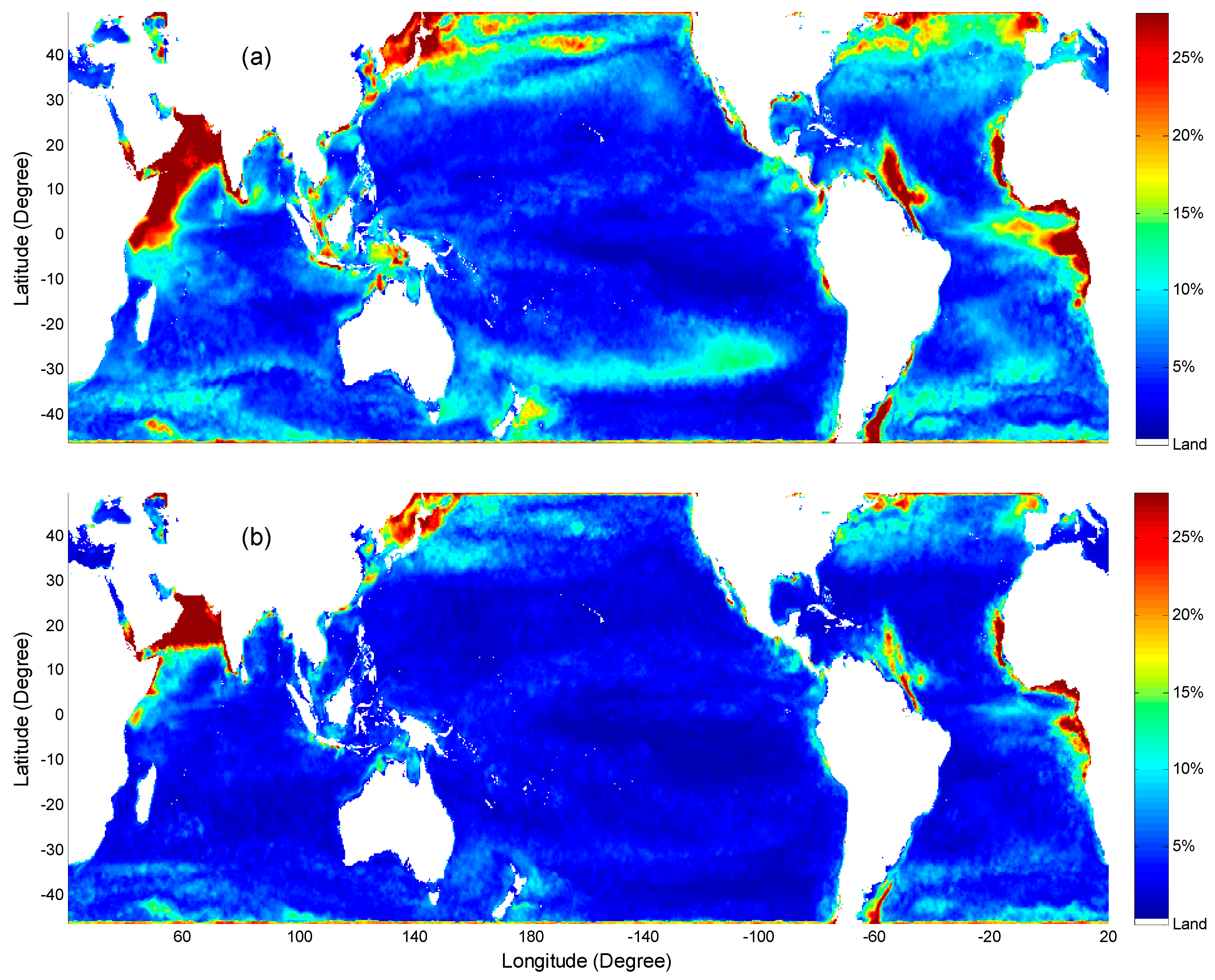
2.4. The Mean Relative Difference

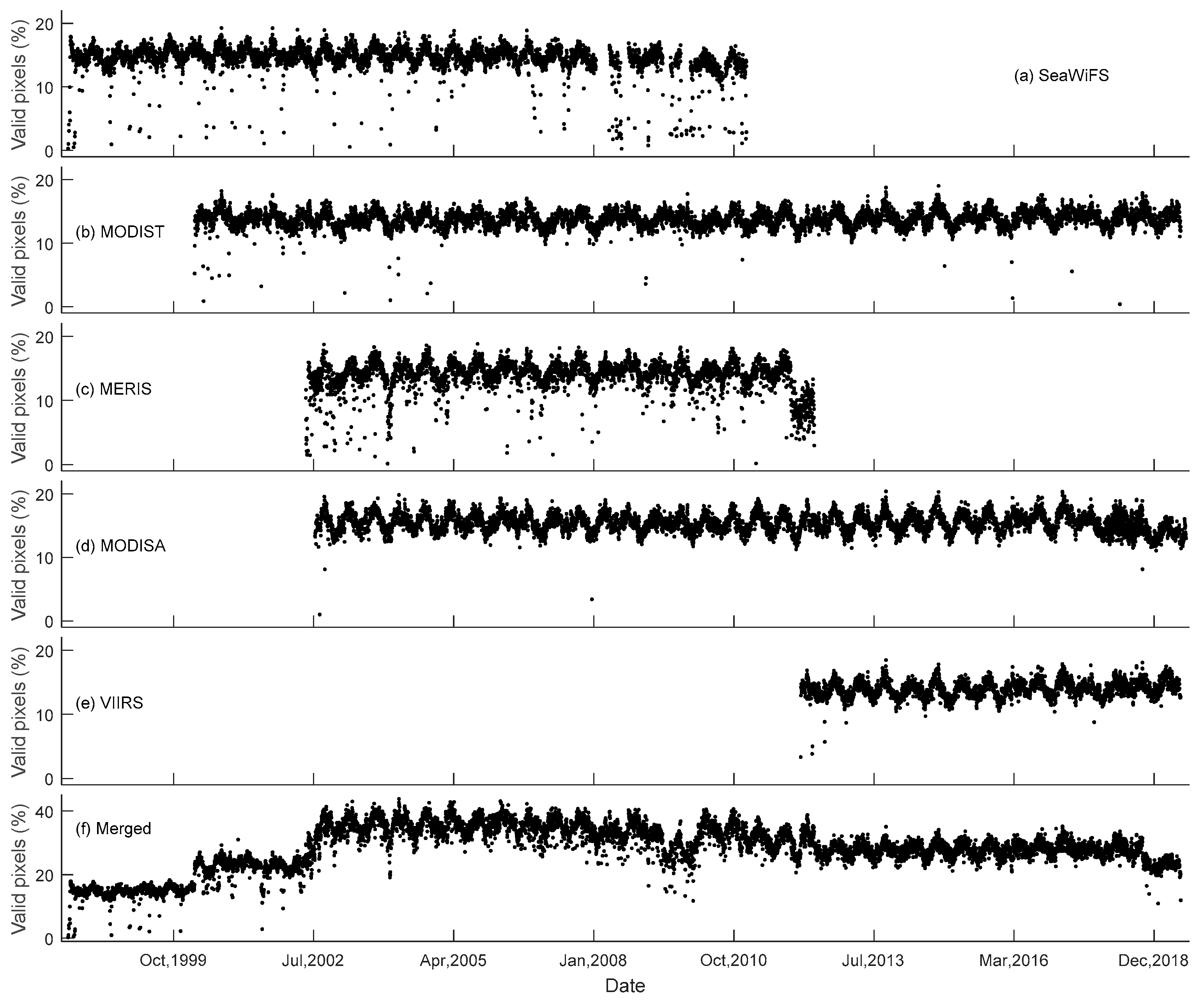
To verify the relevance of using sine functions to approximate the Chl-a, we calculated the Mean Relative Difference (MRD) between the fitted value and the Chl-a climatology as:

$$\mathrm{MRD}=100\times \mathrm{mean}(|\frac{\mathrm{y}\left(\mathrm{t}\right) - \mathrm{x}\left(\mathrm{t}\right)}{\mathrm{x}\left(\mathrm{t}\right)}|),$$

(4)

where $\mathrm{y}\left(\mathrm{t}\right)$ is the fitted value, $\mathrm{x}\left(\mathrm{t}\right)$ is the satellite Chl-a on the same day and same location.

2.5. Data

The phytoplankton biomass is commonly indexed by Chl-a, estimated from ocean color remote sensing data [35]. In this study, we used satellite-retrieved Chl-a data including Sea-Viewing Wide Field-of-View sensor (SeaWiFS, 1997–2010), Moderate Resolution Imaging Spectroradiometer on Terra (MODIST, 1999–present) and Aqua (MODISA, 2002–present), Medium Resolution Imaging Spectrometer (MERIS, 2002–2012), and Visible Infrared Imaging Radiometer Suite (VIIRS, 2011–present). These data were downloaded from the website (http://oceancolor.gsfc.nasa.gov), as listed in

Table 1. Overall information of Chlorophyll-a concentration (Chl-a) dataset from five satellites.

Satellite	Date	Number of Days
SeaWiFS	4 September 1997–11 December 2010	4488
MODIST	24 February 2000–3 June 2019	6953
MERIS	9 April 2002–8 April 2012	3502
MODISA	4 July 2002–9 July 2019	6465
VIIRS	2 January 2012–8 June 2019	2681

. The data quality has been evaluated by lots of regional and global in-situ measurements [6,22,36]. The data are the global daily Chl-a of level-3 products and binned into the same pixel resolution of approximately 9 km × 9 km.

From Table 1, the length of satellite observation varies from eight years for VIIRS to almost twenty years for MODIST. The MODISA, MODIST, and VIIRS satellites are still operating. The end dates for these satellites in Table 1 are the periods of data downloaded from the web. There is a total of 24,089 files which are merged into 7956 daily files. These five satellites together provide continuous measurements of Chl-a from September 1997 to June 2019. As they cannot measure Chl-a in the presence of clouds and other factors, there are many empty values in the daily images of Chl-a. The percentages of valid pixels are relatively low, as shown in Figure 1, where the percentages are computed from the ratio of the number of valid pixels to the number of the global ocean pixels.

From Figure 1, the daily percentages of valid pixels of each satellite exhibit seasonal changes which are mainly due to seasonal variability of the coverage of the incident solar irradiance on the sea surface. The numbers of valid satellite-retrieved Chl-a are also affected by the satellite swath, data processing algorithms, the cloud coverage, thick aerosols, sun glint, and other factors. The percentage of valid pixels of each satellite ranges from 10% to 20% with the average of 14.5% (SeaWiFS), 15.4% (MODISA), 13.8% (MODIST), 13.8% (MERIS), and 14.0% (VIIRS), respectively. The valid pixel coverage of Chl-a images of Level 3 products between MERIS and MODIS are similar, even though there is a large difference of satellite swath between about 1000 km of MERIS and about 2000 km of MODIS.

Figure 1 shows that more than two satellites simultaneously have measured the ocean since 2000 and four satellites together between 2002 and 2010. The percentage of merged data shows that the numbers of valid pixels increase with the increasing numbers of satellites. It is about 22.5% for two satellites together, 27.9% for three, and 33.6% for four satellites. The average of valid pixels of the merged files is 28.3%, indicating most areas filled by empty values. The low coverage of valid pixels may produce remarkable errors in timing of phenological metrics [5].

To increase the percentage of valid pixels, the composite images of 8-day and monthly are usually produced but some regions are still covered by invalid pixels. To solve this issue, the climatological imagery offers another way to significantly increase the percentage of valid data. Yoder et al. [1] used the monthly climatological mean of the Coastal Zone Color Scanner data to analyze the seasonality. Westberry et al. [37] constructed climatology from 8-day composites of MODIS data over a 10-year period averaged over 5° × 10° boxes. Sapiano et al. [22] established a global climatology of phytoplankton to better understand the timing of phytoplankton. Friedland et al. [31] used GSM merged data product to examine the dominant phytoplankton blooms. A daily climatology was produced from the merged files by averaging Chl-a values on the same day of years between 1997 and 2019. For the leap years, the files of Day 366 are merged into the image of Day 365. This climatology is composed of a time series of 365 images with the pixel resolution of approximately 9 km × 9 km.

3. Results and Discussion

3.1. The Parameters of the Nonlinear Fit Function

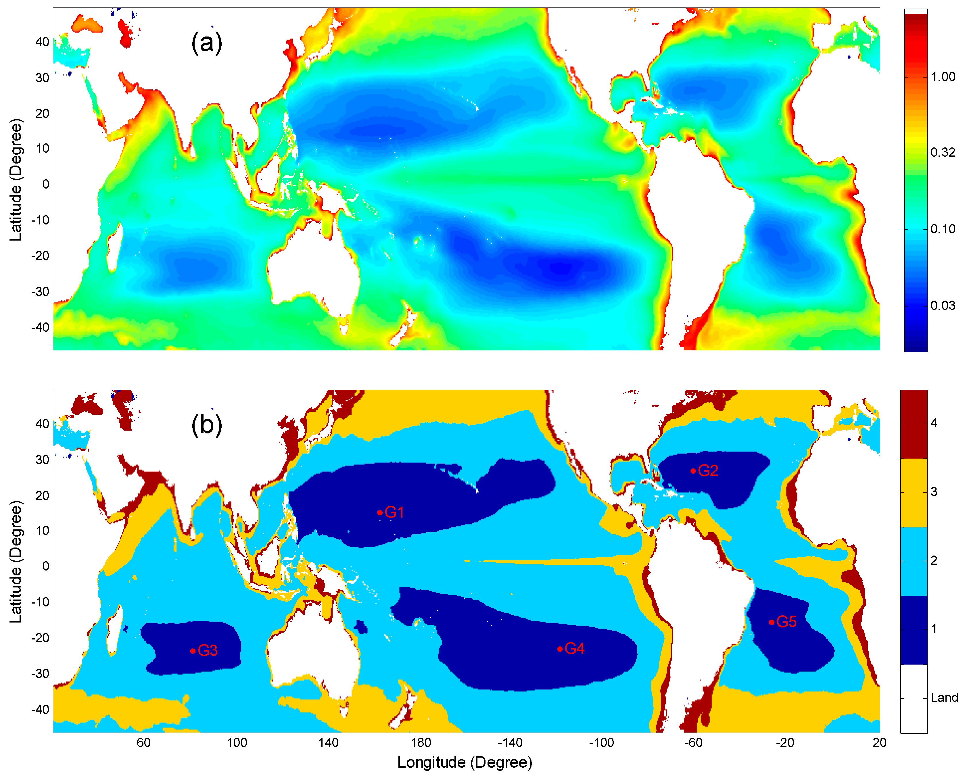
The nonlinear fit function is used to obtain the parameters of mean, amplitude, and phase from the time series of daily climatological Chl-a. The frequency is implied in different numbers of cycles, representing seasonal characteristics with corresponding time periods.

3.1.1. Mean Chl-a

When Equation (1) is used to fit the time series of climatological Chl-a, we obtain the overall average of all Chl-a data (1997–2019), as shown in Figure 2a. The latitude range is limited within 48°N to 48°S because satellite Chl-a data of higher latitudes are not available in some seasons.

As can be seen in Figure 2a, the average of Chl-a exhibits remarkable spatial difference and can be used to separate several different regions. A striking feature is the five subtropical gyres with the lowest primary productivity that have been referred to as “ocean deserts” [38]. They did not change greatly across the seasons [39], but they are strongly influenced by vertical mixing and nutrient delivery [30]. The centers of the gyres are easily located and displayed in Figure 2b with Chl-a of 0.033 mg/m³ (G1), 0.043 mg/m³ (G2), 0.044 mg/m³ (G3), 0.022 mg/m³ (G4), and 0.036 mg/m³ (G5), respectively. When Chl-a is less than the threshold of 0.07 mg/m³ (which is used to detect oligotrophic gyres, Polovina et al. [10]), the regions are identified as Class 1 in Figure 2b and the areas of the gyres are 20.94 × 10⁶ km² (North Pacific Ocean), 5.97 × 10⁶ km² (North Atlantic Ocean), 6.10 × 10⁶ km² (South Indian Ocean), 19.75 × 10⁶ km² (South Pacific Ocean), and 6.49 × 10⁶ km² (South Atlantic Ocean), respectively. The total area of the gyres is 59.26 × 10⁶ km², comprising ∼16.5% of the ocean.

Due to large terrestrial nutrient input and strong coastal mixing, the marginal seas have higher growth rate of phytoplankton leading to larger values of Chl-a [18,40]. Some large values are produced because Chl-a is often challenging to extract in coastal regions given the spatio-temporal optical complexity of these waters [41]. If Chl-a > 0.5 mg/m³, these regions can be identified as Class 4 in Figure 2b. The other oceans are classified as Class 2 and 3 using the threshold of 0.2 mg/m³ which was used to identify the chlorophyll isopleth for the Transition Zone Chlorophyll Front (TZCF) [10]. The TZCF is the interface between the low-surface chlorophyll subtropical gyre and the high surface chlorophyll subarctic gyre with features driven by the dynamics of very specialized oceanic habitats [10].

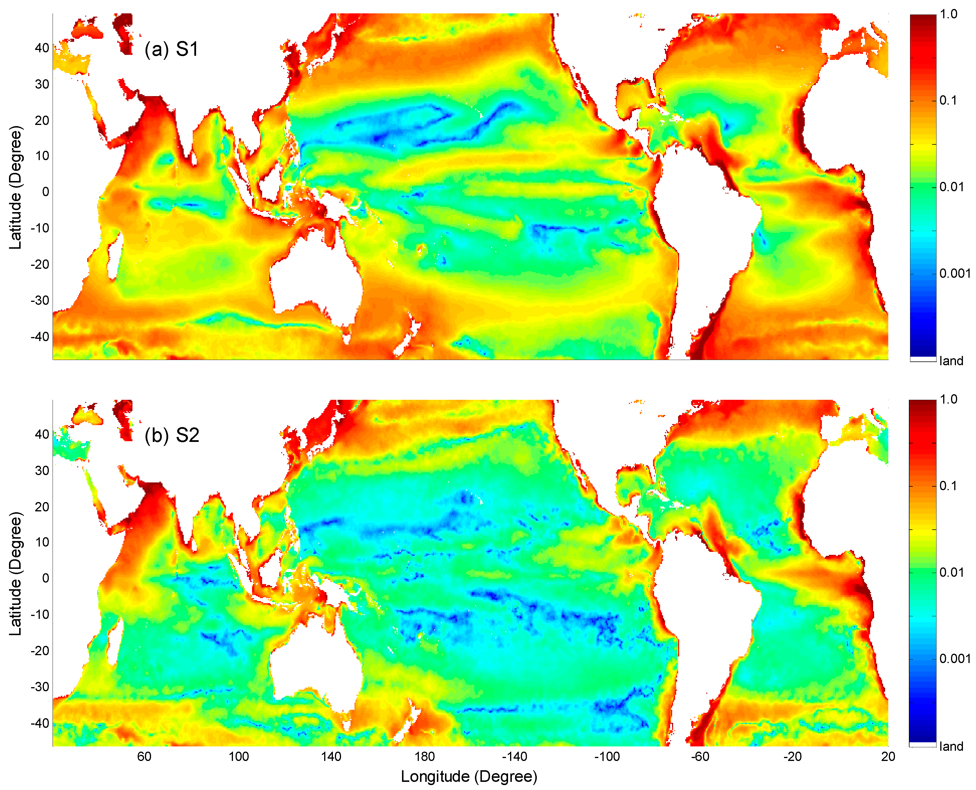
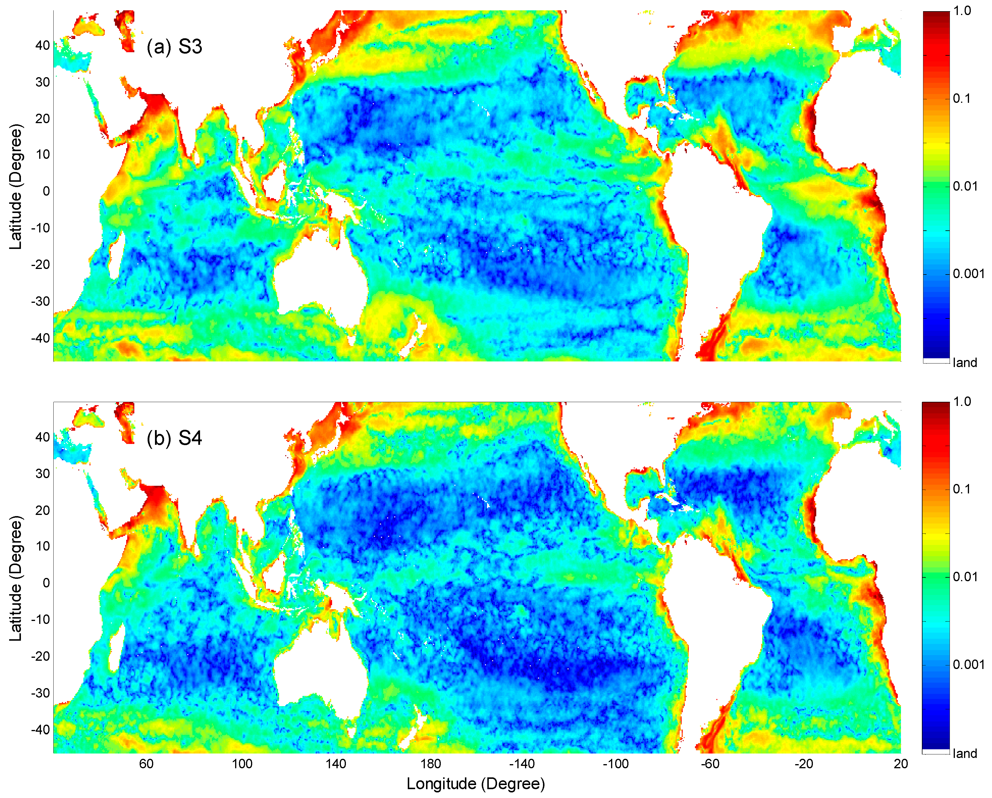
3.1.2. Amplitudes of Different Cycles

When Equation (2) is used to fit the daily climatology of Chl-a images, the amplitudes of S1 and S2 are obtained, as shown in Figure 3. The amplitude image of S1 in Figure 3a is the spatial patterns of the parameter A for all three equations and the image of Figure 3b is that of the parameter B for Equations (2) and (3). These two amplitude images can also be obtained from the FFT (Fast Fourier Transformation) analysis.

Large amplitudes indicate strong seasonal variability of Chl-a that is mostly distributed in coastal and oceanic frontal regions. Some remarkable patterns of high values are consistent with the TZCF regions. The estimated horizontal transport of nitrate in the regions of TZCF supports up to 40% of new primary productivity annually and nearly 100% in the winter [42]. The TZCF regions seasonally migrate between the two pelagic ecosystems on temporal scales which can be reflected by the amplitudes. For example, the patterns of amplitude images in the North Pacific Ocean are spatially consistent with the range of TZCF that seasonally migrates over 1000 km from its southernmost position during the first quarter of the year at about 30–35°N to its northernmost position during the third quarter of the year at about 40–45°N [10].

Comparing Figure 3 to Figure 2, the patterns of amplitudes are different from that of the mean image. The regional patterns of the five subtropical gyres become complicated in the images of the amplitudes, indicating that the seasonality of Chl-a is different among these gyres and varies in a relatively complicated way. Combining Figure 2 and Figure 3, the images of amplitudes offer a way to distinguish the seasonal variations from the background of Chl-a in different regions. When Equation (3) is used to fit the daily climatology, the amplitudes of S3 and S4 are obtained, as shown in Figure 4. S3 and S4 represent seasonal variations of components with a period of four and three months.

The amplitudes of the different cycles actually represent the temporal variations of Chl-a with respective time periods. The magnitudes of S1 are the largest, indicating that the annual cycle of phytoplankton dominates the seasonal variability [9]. The patterns become more regionally scattered from S1 to S4, indicating that amplitudes become more regional with shorter time periods (inter-annual), especially in the equator regions. The regions with low values (<0.01 mg/m³) of S1 amplitude are spatially consistent with those marked as Models 1 and 2 of Sapiano et al. [22], where the two models imply no statistically significant cycles. In fact, the patterns of S1 in these regions are still very complicated and some remarkable patterns can also be identified from the amplitude images of S2 and S3. It implies that the seasonal cycles of phytoplankton can still be identified from these amplitude images in these regions.

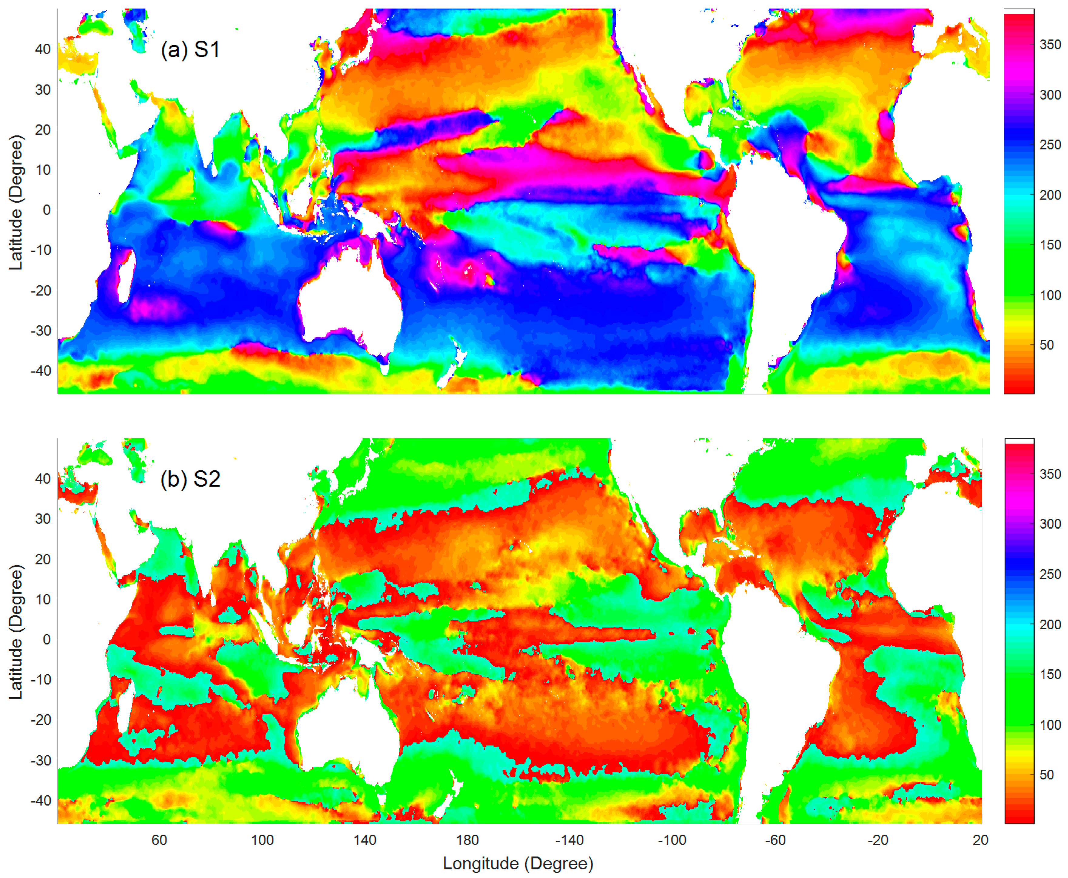
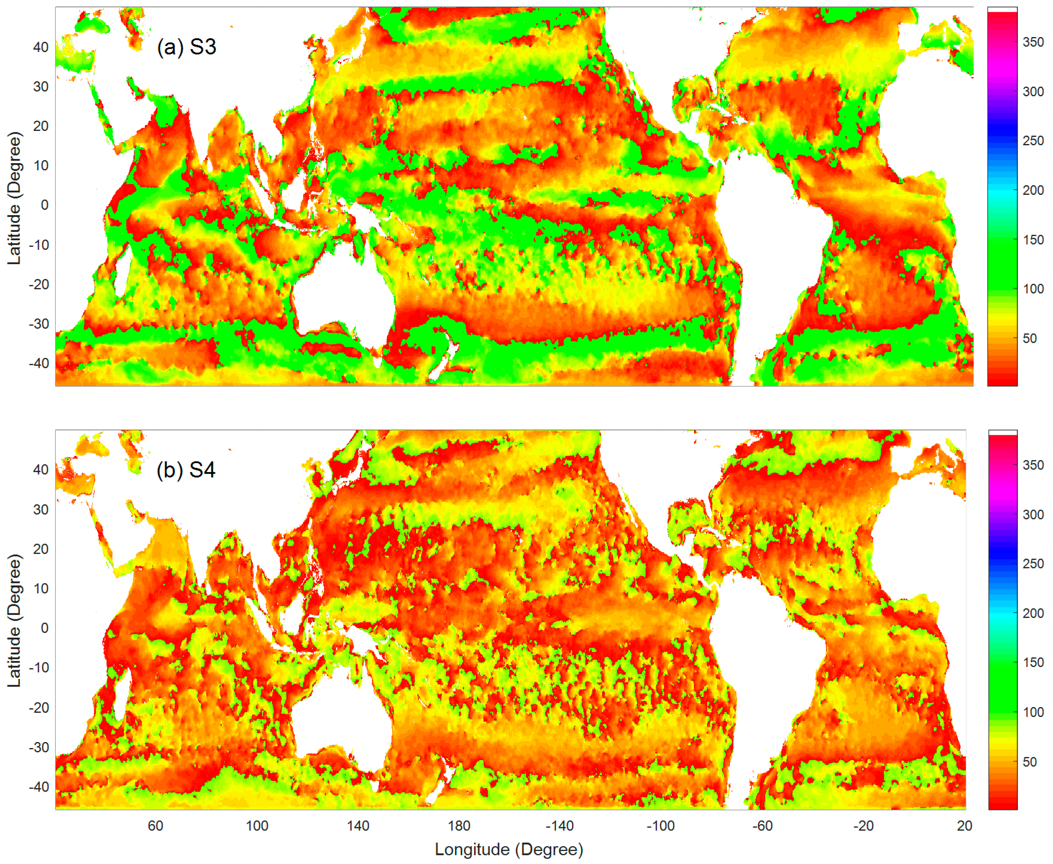
3.1.3. Phases of Different Cycles

Similar to the amplitude, two phases are obtained from Equation (2), as shown in Figure 5. The unit of phase is converted to the day of year. These phase images can also be obtained from the FFT analysis.

From Figure 5a, values of $\mathrm{S}$1 in the Northern Hemisphere (NH) are essentially 180° transitions of that in the Southern Hemisphere (SH), indicating that blooms of the NH occur seasonally inverse with those of the SH, similar to the results of Sapiano et al. [22]. It implies that the annual cycle of phytoplankton may be mainly controlled by the seasonal light intensity coverages of incident solar irradiance on the sea surface during the period of the year. The underlying dynamics influencing the timing of the blooms is highly complex, which also depends on nutrient availability, temperature among others [9]. Conversely, intensified light and warm temperature stimulate the growth of phytoplankton, while the shallow mixed layer limits the supply of nutrients from subsurface, which in return limits the growth of phytoplankton [14]. There are some exceptions, for example, values of $\mathrm{S}$1 in latitudes (40°N–48°N) are significantly different from that in temperate domains. In Figure 5b, the most spatially contrasted values of the image pattern are the difference between low latitudes (<30°) and high latitudes, indicating the timing of bloom onset increases with higher latitudes. Similarly, the phases of $\mathrm{S}$3 and $\mathrm{S}$4 can be obtained from Equation (3), as shown in Figure 6.

Comparing the images of four phases, the pattern of $\mathrm{S}$1 exhibits regional homogeneity and that of S4 becomes scattered. The patterns of $\mathrm{S}$3 mainly correspond to the seasonal variations of the TZCF regions and the S4 exhibits much more local/regional variability. Therefore, the patterns of phases reveal the seasonal cycles with different time periods, which are varying in space.

Comparing images between phase and amplitude, values of amplitudes in the coastal regions are higher than other regions, while spatial patterns of four phases are seldom affected by the coastal waters. The image patterns of S1 phase are similar to the results of phenological timing of Racault et al. [43]. As the phase values are determined on the zero $\mathrm{S}$1 values when the sinusoid crosses from negative to positive, indicating the phases can be used to determine the timing of bloom onset.

3.2. Comparison of Different Sine Equations

Equations (1)–(3) can produce fitted values of Chl-a and be compared to satellite climatology data. The MRD (Equation (4)) is used to compute the difference between the fitted values and satellite data for assessing the performance of the equations. The MRD values of Equations (1) and (2) are computed and shown in Figure 7.

The patterns of MRD images show regional distribution with large values in coastal and frontal regions. Large values in the north of the Arabian Sea are due to the low coverage of valid data. For other coastal regions with large values, the most possible reason is that phytoplankton growth in these regions is affected by the multitude of regional factors and has no obvious periodic variations. However, the values of Equation (1) in the most areas are less than 10%, indicating that the fitted values of the sine equation match the satellite data with a global average of 7.1%. Comparing Figure 7b with Figure 7a, the MRD values of Equation (2) become smaller with a mean of 4.5%. The MRD image of Equation (3) is shown in Figure 8a. To compare the MRD values of the three equations, a classified image based on the different ranges of MRD values is shown in Figure 8b, where the difference of MRD of the three equations is classified as four classes using the threshold of 5%.

Comparing Figure 8a to Figure 7, the MRD values of Equation (3) become much smaller than the other two equations. The average of MRD is 3.3%, indicating that Equation (3) can significantly reduce the difference between the fitted values and the climatology, but there are only about 3.6% areas with MRD values >10% in some coastal regions. Some tests have been carried out by the use of more sinusoids, indicating that MRD values are reduced in very small ranges (not shown here). From Figure 8b, the areas with small MRD values (defined as less than 5%) significantly increase from Equations (1)–(3), which are 44.3% (Equation (1)), 76.5% (Equation (2)), and 87.3% (Equation (3)), respectively. Therefore, Equation (3) can match the patterns of daily climatology with small MRD values over approximately 90% of oceans.

To examine the matching situations of the different equations in detail, the fitted values of three equations (y1–y3) with the satellite data against the day of year for one example of each class (E1–E4, please refer to Figure 8b for their locations) are shown in Figure 9. The shapes of the seasonal cycles of Chl-a at the four sites in the North Pacific Ocean are different from each other. It is easy to see that the seasonal variations at E1 and E2 have an annual cycle, while E3 and E4 have a semiannual cycle.

For annual cycle at site E1 (Figure 9a), the three fitted values can match the satellite climatology (Sat) with MRD values of 2.3%, 1.8%, and 1.1%, respectively. The matching situations are similar in other sites of Class 1, indicating that all three equations can be used to fit the time series of climatology over about half areas of oceans. For annual cycle at site E2 (Figure 9b), the two MRD values (Equations (2) and (3)) are still small with values of 3.2% and 1.9%, but that of Equation (1) becomes large (10.1%). The large MRD value is due to some discrepancies between Equation (1) and the shape of Chl-a when the width of the peak of satellite data is much shorter or longer than that of valley. For semiannual cycle at site E3 (Figure 9c), Equation (1) obviously produces large differences with the MRD of 10.5%, and the differences of Equation (2) are also large (8.1%), but the matching situation has been significantly improved by Equation (3) (3.8%). It demonstrates that Equation (3) can adjust the shape of sines to match the pattern of the climatology. For coastal regions at site E4 (Figure 9d), the differences of all three fitted values are relatively large with MRD values of 24.7% (Equation (1)), 23.4% (Equation (2)), and 10.3% (Equation (3)), respectively.

3.3. The Effects of Climatology on Seasonal Cycles

We have established a climatological dataset from the five satellite-retrieved Chl-a and used sine equations to fit the seasonal variability. To examine the relationship between the climatology and satellite-retrieved Chl-a, the climatological values are compared to all satellite-retrieved data at four sites (E1–E4 marked in Figure 8b) against the day of year, as shown in Figure 10.

In Figure 10a, there are 611, 734, 463, 772, and 300 dots for SeaWiFS, MODIST, MERIS, MODISA, and VIIRS, respectively. The mean numbers of dots on one day of year are very small with the average of 1.7, 2.0, 1.3, 2.1, and 0.8 for these five satellites. The numbers become smaller for site E3 (Figure 10c) with the average of 0.5, 1.1, 0.7, 1.1, and 0.4, respectively. The different numbers among different satellites are mainly due to different period of satellite data. The differences between E1 and E3 are mainly due to the different coverage of clouds and other factors such as the effects of the sun glint. As these satellites have run more than ten years, it indicates that one satellite measures Chl-a only about one time during a period of ten years at a fixed pixel. This result is consistent with the spatial coverage of valid pixels for one satellite (about 14%). However, the daily climatology offers a gap-free coverage of the Chl-a dataset.

Comparing the patterns of climatology to satellite data in Figure 10, the climatology is around the centers of dots of satellite-retrieved Chl-a according to the day of year. The dot patterns of the satellite-retrieved are much more scattered than that of the climatology. For site E1 in Figure 10a, the MRD values are 15.9%, 15.4%, 19.8%, 17.3%, and 16.8%, for SeaWiFS, MODIST, MERIS, MODISA, and VIIRS, respectively, much larger than that of the climatology (1.1%). The MRD values at site E2 are 16.2%, 18.3%, 22.5%, 16.8%, and 17.6%, respectively, also much larger than that of the climatology (1.9%). It demonstrates that the MRD values of the satellite-retrieved Chl-a images will be large when they are directly used to obtain the fitted values instead of the daily climatology. Values of the climatology are actually the means of satellite data on the same day of year and can remarkably reduce the variability of the satellite-retrieved Chl-a, clearly exhibiting the seasonal patterns of phytoplankton. Notably, the use of climatology will lose the capability to capture some natural phenomena such as detecting red tides. However, the red tides may be easily identified if climatology is taken as a reference, which is also beneficial for comparing the seasonal variations of blooms between different years.

In Figure 10b, the annual cycle can be identified directly from the dot pattern of satellite-retrieved Chl-a. The difference between maximum and minimum of climatology reaches up to 0.2 mg/m³, much larger than the average of the standard deviations (STD) of satellite-retrieved Chl-a on the same day of year which is 0.05 mg/m³. It demonstrates that a larger seasonal change at a specific location makes it easy to identify the seasonal cycles from the dot patterns of satellite-retrieved Chl-a. From Figure 10a, the difference between maximum and minimum of fitted values is 0.03 mg/m³ while the STD average of satellite-retrieved Chl-a reaches up to 0.15 mg/m³. It causes the difficulty to identify the seasonality directly from the dot patterns of satellite-retrieved values. However, the seasonal cycles can still be easily identified from the shape of time series of climatology. Therefore, the climatology can exhibit the seasonal patterns much more clearly than that of the satellite-retrieved Chl-a.

As the specifications of the satellite sensors and data processing systems differ with each other, the data quality of each satellite-retrieved Chl-a is also different. To understand the performance of each satellite, the fitted values of Equation (3) are used to compute the MRD values of satellite-retrieved Chl-a based on the same pixel and same day of year, as shown in Figure 11. The merged image is computed from the composite imagery which are the average of five satellites on the same day.

Figure 11 shows that the patterns of MRD images are similar to each other except for MERIS. These patterns are also similar to that of amplitude image of S2 in Figure 3a. It demonstrates that large MRD values are caused by the temporal variability of satellite-retrieved Chl-a of different years over the coastal and frontal zones. The mean MRD values of the images are 16.6%, 15.9%, 20.8%, 16.8%, 17.0%, and 17.4% for SeaWiFS, MODIST, MERIS, MODISA, VIIRS, and merged data, respectively. The value of MERIS is the largest due to its spatial/temporal characteristics of images being substantially different from the other four satellites. However, these results cannot be used to evaluate the actual accuracy of each satellite because we take the fitted values of Equation (3) as the “truth value”, which is actually the average of satellite data. As MERIS takes only a small part (about 15%) of the dataset and other satellites are similar, it may cause the patterns of MERIS in Figure 11 to differ from the others. It also causes the MRD of merged data less than that of MERIS but larger than the others. We also use Equation (2) to compute MRD values with similar image patterns of Figure 11. The mean MRD values are 16.8% (SeaWiFS), 16.0% (MODIST), 20.9% (MERIS), 16.9% (MODISA), 17.2% (VIIRS), and 17.5% (Merged), respectively. Compared to the MRD value of the daily climatology (3.3%), the climatology can significantly reduce the MRD values of satellite data.

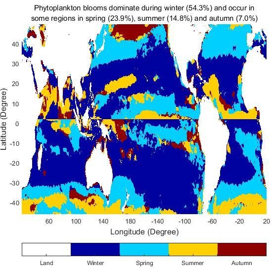
3.4. The Timing of Phytoplankton Blooms

Phytoplankton blooms are a recurrent feature each year and play an important role in oceanic uptake of atmospheric carbon dioxide and fishery stocks [37,44]. The phytoplankton bloom can be identified by the maxima of Chl-a [45]. In fact, there are many abnormal values in satellite Chl-a, easily obtaining a wrong bloom time identification. When the climatology is fitted by the sine equations, the bloom period can be exactly identified by the biggest peak of the fitted values, as shown in Figure 12a.

The patterns of bloom timing (Figure 12a) are similar to that of S1 phase in Figure 4a, indicating that the global bloom is mainly controlled by the rhythm of S1. The spatial distributions are similar to the patterns of bloom time of Sapiano et al. [22], but our results exhibit the patterns in more details. The image shows that the bloom timing exhibits a smooth shift in some regions, for example, the date of bloom shifts from Day 37 to Day 105 in the Mediterranean Sea, similar to that of Salgado-Hernanz et al. [6]. The bloom timing shifts from Day 1 to Day 180 with increasing latitudes in the North Atlantic Ocean, similar to that of Land et al. [46]. Values in the Japan Sea are smoothly distributed, similar to that of Yamada et al. [44]. The image also shows that the bloom time varies with latitude, which is consistent with Boyce et al. [30] and Friedland et al. [31]. It should be pointed out that the result for the timing of blooms (Figure 12) in this work is applied to the daily climatology, not any particular year of data record. Thus, variations of timing of blooms from year to year cannot be inferred from these results.

Figure 12a also shows spatial discontinuity in some regions, which indicates the timing transitions mainly caused by the switch of magnitudes of two peaks. For example, blooms occur during spring and autumn in the North Pacific Ocean with latitudes higher than 40° and magnitudes of two peaks often switched in a small region. The discontinuity patterns also occur in Chl-a frontal regions such as the equatorial regions, the TZCF, southeast of Vietnam coast, and Boundary Current Systems [28,47,48].

To understand the bloom period distributions more clearly, the regions are classified into four seasons which are adjusted to be boreal seasons for the NH and austral seasons for the SH, as shown in Figure 12b. The results show strong regional distributions and the areas of different seasons vary greatly. The underlying dynamics influencing the timing of the blooms is highly complex, which largely depends on nutrients, light and temperature and the inter-relationship among them. Firstly, the growth of phytoplankton is directly related with the availability of nutrients, which usually limits the growth the phytoplankton. Secondly, suitable light and temperature are fundamental for the growth of phytoplankton and they are tightly connected to each other. During winter for each hemisphere, both the light intensity and temperature are low and less suitable for the growth of phytoplankton. As spring approaches, light intensifies and temperature increases, which stimulates the growth of phytoplankton. The process continues into summer when the strong heat flux leads to shallow mixed layer, thus the supply of nutrients from subsurface is largely reduced, which in return limits the growth of phytoplankton. During fall, when the temperature and light relax, the phytoplankton reduces again. Thus, the initiation and termination times of blooms are related to the light and temperature when nutrients are abundant or deplete. It causes the timing of blooms to strongly depend on geophysical locations and blooms occur in all four seasons. Blooms dominate during boreal winter in about half of the areas (50.6%) in the NH and austral winter in the SH (58.0%). Spring blooms distribute around many regions in the NH (25.5%) and in the SH (22.2%). Summer blooms occur in some areas in the NH (15.8%) and in high latitudes in the SH (13.9%). Autumn blooms seldom occur in the NH (8.1%) and in the SH (5.9%). The above percentage is computed independently on the separation of the ocean between the NH and SH.

3.5. The Effects of Equation (3) on Four Sinusoids

When we check the shapes of the time series of climatology, they exhibit complicated and various kinds of patterns. As the shapes of sinusoids exhibit strictly cyclicity, we wonder whether the sine equations can match the various patterns. To demonstrate it, the climatology and the fitted values of Equation (3) together with four components at four typical sites (P1–P4 with locations marked in Figure 12b) are shown in Figure 13. The four sites, located in the low latitude domains of the Northern Atlantic Ocean, are selected from four different seasons of phytoplankton blooms in order to check the timing of blooms in detail.

To examine the results of Figure 12, the climatology and the fitted values of Equation (3) at four typical sites (P1–P4) are shown in Figure 13. It is easy to identify the bloom time from the biggest peak of both the climatology and the fitted values, but it may be wrongly determined when unexpected noise arises in the climatology, for example, the shape of P4 in Figure 13a. As the fitted values take over the overall shape of the time series of climatology, the results of bloom timing of Equation (3) are very robust and immune from noise. From the time of the biggest peak of the patterns in Figure 13b, the bloom timings of the four sites are Day 32 (1 February), 85 (26 March), 216 (4 August), and 256 (13 September), corresponding to the boreal seasons of winter, spring, summer, and autumn, respectively. Therefore, the fitted values of Equation (3) are suitable to determine the bloom timing of the normal biomass seasonality.

Comparing the shapes of the four components (Figure 13c–f) with that of Equation (3), the patterns are completely changed and become simple. The shape of S1 at P1 is similar to that of P2, but the shapes of P1 and P2 are remarkably different. The shape of S2 at P1 and P2 is close, but it is difficult to be identified from the shapes of climatology. It similarly occurs for that of P3 and P4. The four components (S1–S4) may exhibit some implications of seasonal characteristics of climatological Chl-a with different time periods. For example, the site P4 reflects the offshore region of the Amazon River and the chlorophyll can be impacted by nutrient, light and also river discharge. As more sinusoid is being used, the timing of blooms can be more exactly identified, and the greater number of peaks of Chl-a within a year can be reflected by the fitted values. Therefore, Equation (3) can be used to derive the images of four sinusoids, which are ecologically important to determine some phenological characteristics.

In Figure 13b, the patterns of Equation (3) at the four sites are significantly different and they are all beyond the shape of sinusoids, but they can match the patterns of climatology (Figure 13a) very well with relatively small MRD values. The combinations of four sinusoids can adjust the shapes of the fitted values to match the patterns of the climatology. Therefore, Equation (3) can be used to match the various patterns of the time series of daily Chl-a climatology.

4. Conclusions

The seasonal variability of Chl-a is complex, and the low coverage of satellite-retrieved data have limited the understanding of seasonality of phytoplankton. Some noises in satellite data will lead to wrong determinations of phenological characteristics. When satellite data are used to produce the daily climatological imagery, which are the average of satellite Chl-a on the same pixel and the same day of years during the period of 1997–2019, the climatology can significantly reduce the variability of satellite values and clearly exhibit the seasonal cycles. The fitted values of sine equations can reflect the overall shapes of seasonality of phytoplankton and offer a time series of Chl-a baseline as a standard reference describing the normal state of seasonal cycles of phytoplankton.

Three types of sine equations were used to examine their relevance to approximate the daily climatology and our results show that Equation (3) with four sinusoids can match various patterns of the time series of climatological imagery with MRD of 3.3%. The functions can derive the parameters of mean, amplitude, phase and frequency for describing the phenological characteristics. The mean image offers an overview background of Chl-a patterns during the period of 1997–2019 and is used to classify the global ocean into four different regions. The four amplitude images of Equation (3) reflect spatial magnitudes of seasonal variations with different periods and high values exhibit the spatial distribution of the coastal and frontal zones. The four phase images reflect the initiation time of biomass with different periods and the values can be used for the study of the phonological metrics.

Equation (3) can significantly improve the matching situations of both because the addition of other sinusoids (T3 and T4) can adjust the shapes of the fitted values to match various patterns of daily Chl-a climatology (and to take inter-annual variability into account). The three equations have limitations in matching strong blooms with a short period and MRD values cannot be significantly reduced with more sinusoid functions due to the repeated cycles of the sinusoids in the whole year. However, the timing of the blooms can still be exactly captured by Equation (3) and its derived parameters can be used to determine the phonological metrics. A combination of sinusoids and other functional forms such as Gaussian function can be used to describe the patterns with sudden blooms such as red tides.

The timing of the main blooms can be located by positions of the maxima of the fitted values of Equation (3). Our results show that blooms occur in all four seasons over the global ocean with the seasonality of geophysical features. Blooms dominate during austral winter (June–August) in most regions in the SH (58.0%) and about half of the oceans in the NH (50.8%) during boreal winter (December–February) in the latitude domains (48°N–48°S), as winter blooms generally occur at subtropics with the extensive oligotrophic gyres when the water stratification is weak and the nutrients can be transported to the surface waters easily. Blooms occur in many regions during boreal spring in the NH (25.5%) and austral spring in the SH (22.2%), as spring blooms generally occur at subpolar and higher latitudes which can be explained by the critical depth hypothesis. Blooms seldom occur during austral autumn in the SH (5.9%) and boreal autumn in the NH (8.1%). In fact, both spring and autumn blooms may occur at temperate latitudes, as can be observed with the Japan Sea. The autumn bloom is typically less intense than the spring bloom. It is mainly induced by the intensification of wind before light becomes a limiting factor. The detailed mechanism should be further studied in the future.

References

1. Yoder, J.A.; McClain, C.R.; Feldman, G.C.; Esaias, W.E. Annual cycles of phytoplankton chlorophyll concentrations in the global ocean: A satellite view. Glob. Biogeochem. Cycles 1993, 7, 181–193. [Google Scholar] [CrossRef]
2. Moore, J.K.; Abbott, M.R. Phytoplankton chlorophyll distributions and primary production in the Southern Ocean. J. Geophys. Res. Space Phys. 2000, 105, 28709–28722. [Google Scholar] [CrossRef]
3. Behrenfeld, M.J.; O’Malley, R.T.; Siegel, D.A.; McClain, C.R.; Sarmiento, J.L.; Feldman, G.C.; Milligan, A.J.; Falkowski, P.G.; Letelier, R.M.; Boss, E. Climate-driven trends in contemporary ocean productivity. Nature 2006, 444, 752–755. [Google Scholar] [CrossRef] [PubMed]
4. Vantrepotte, V.; Mélin, F. Inter-annual variations in the SeaWiFS global chlorophyll a concentration (1997–2007). Deep Sea Res. Part I Oceanogr. Res. Pap. 2011, 58, 429–441. [Google Scholar] [CrossRef]
5. Cole, H.; Henson, S.A.; Martin, A.; Yool, A. Mind the gap: The impact of missing data on the calculation of phytoplankton phenology metrics. J. Geophys. Res. Space Phys. 2012, 117. [Google Scholar] [CrossRef]
6. Salgado-Hernanz, P.; Racault, M.-F.; Font-Muñoz, J.; Basterretxea, G. Trends in phytoplankton phenology in the Mediterranean Sea based on ocean-colour remote sensing. Remote Sens. Environ. 2019, 221, 50–64. [Google Scholar] [CrossRef]
7. Platt, T.; White, G.N.; Zhai, L.; Sathyendranath, S.; Roy, S. The phenology of phytoplankton blooms: Ecosystem indicators from remote sensing. Ecol. Model. 2009, 220, 3057–3069. [Google Scholar] [CrossRef]
8. Cushing, D.H. The seasonal variation in oceanic production as a problem in population dynamics. ICES J. Mar. Sci. 1959, 24, 455–464. [Google Scholar] [CrossRef]
9. Behrenfeld, M.J.; Randerson, J.T.; McClain, C.R.; Feldman, G.C.; Los, S.O.; Tucker, C.J.; Falkowski, P.G.; Field, C.B.; Frouin, R.; Esaias, W.E.; et al. Biospheric Primary Production During an ENSO Transition. Science 2001, 291, 2594–2597. [Google Scholar] [CrossRef] [Green Version]
10. Polovina, J.J.; Howell, E.; Kobayashi, D.R.; Seki, M.P. The transition zone chlorophyll front, a dynamic global feature defining migration and forage habitat for marine resources. Prog. Oceanogr. 2001, 49, 469–483. [Google Scholar] [CrossRef]
11. Henson, S.A.; Dunne, J.P.; Sarmiento, J.L. Decadal variability in North Atlantic phytoplankton blooms. J. Geophys. Res. Space Phys. 2009, 114. [Google Scholar] [CrossRef]
12. Grodsky, S.A.; Carton, J.A.; McClain, C.R. Variability of upwelling and chlorophyll in the equatorial Atlantic. Geophys. Res. Lett. 2008, 35. [Google Scholar] [CrossRef] [Green Version]
13. Kahru, M.; Gille, S.T.; Murtugudde, R.; Strutton, P.G.; Sarabia, M.M.; Wang, H.; Mitchell, B.G. Global correlations between winds and ocean chlorophyll. J. Geophys. Res. Space Phys. 2010, 115. [Google Scholar] [CrossRef] [Green Version]
14. Navarro, G.; Caballero, I.; Prieto, L.; Vazquez, A.; Flecha, S.; Huertas, I.E.; Ruiz, J. Seasonal-to-interannual variability of chlorophyll-a bloom timing associated with physical forcing in the Gulf of Cádiz. Adv. Space Res. 2012, 50, 1164–1172. [Google Scholar] [CrossRef] [Green Version]
15. Ardyna, M.; Claustre, H.; Sallée, J.-B.; D’Ovidio, F.; Gentili, B.; Van Dijken, G.L.; D’Ortenzio, F.; Arrigo, K.R. Delineating environmental control of phytoplankton biomass and phenology in the Southern Ocean. Geophys. Res. Lett. 2017, 44, 5016–5024. [Google Scholar] [CrossRef]
16. Lan, K.-W.; Shimada, T.; Lee, M.-A.; Su, N.-J.; Chang, Y. Using Remote-Sensing Environmental and Fishery Data to Map Potential Yellowfin Tuna Habitats in the Tropical Pacific Ocean. Remote Sens. 2017, 9, 444. [Google Scholar] [CrossRef] [Green Version]
17. Liao, C.-H.; Lan, K.-W.; Ho, H.-Y.; Wang, K.-Y.; Wu, Y.-L. Variation in the Catch Rate and Distribution of Swordtip Squid Uroteuthis edulis Associated with Factors of the Oceanic Environment in the Southern East China Sea. Mar. Coast. Fish. 2018, 10, 452–464. [Google Scholar] [CrossRef] [Green Version]
18. Yu, Y.; Xing, X.; Liu, H.; Yuan, Y.; Wang, Y.; Chai, F. The variability of chlorophyll-a and its relationship with dynamic factors in the basin of the South China Sea. J. Mar. Syst. 2019, 200, 103230. [Google Scholar] [CrossRef]
19. Yamada, K.; Ishizaka, J. Estimation of interdecadal change of spring bloom timing, in the case of the Japan Sea. Geophys. Res. Lett. 2006, 33, 02608. [Google Scholar] [CrossRef]
20. Zhai, L.; Platt, T.; Tang, C.; Sathyendranath, S.; Hernandez-Walls, R. Phytoplankton phenology on the Scotian Shelf. ICES J. Mar. Sci. 2011, 68, 781–791. [Google Scholar] [CrossRef] [Green Version]
21. Vargas, M.; Brown, C.W.; Sapiano, M.R.P. Phenology of marine phytoplankton from satellite ocean color measurements. Geophys. Res. Lett. 2009, 36, 329–342. [Google Scholar] [CrossRef] [Green Version]
22. Sapiano, M.R.P.; Brown, C.W.; Uz, S.S.; Vargas, M. Establishing a global climatology of marine phytoplankton phenological characteristics. J. Geophys. Res. Space Phys. 2012, 117. [Google Scholar] [CrossRef]
23. Huang, N.E.; Wu, Z. A review on Hilbert-Huang transform: Method and its applications to geophysical studies. Rev. Geophys. 2008, 46. [Google Scholar] [CrossRef] [Green Version]
24. Palacz, A.P.; Xue, H.; Armbrecht, C.; Zhang, C.; Chai, F. Seasonal and inter-annual changes in the surface chlorophyll of the South China Sea. J. Geophys. Res. Space Phys. 2011, 116. [Google Scholar] [CrossRef]
25. Zhang, M.; Zhang, Y.; Qiao, F.; Deng, J.; Wang, G. Shifting Trends in Bimodal Phytoplankton Blooms in the North Pacific and North Atlantic Oceans From Space With the Holo-Hilbert Spectral Analysis. IEEE J. Sel. Top. Appl. Earth Obs. Remote Sens. 2017, 10, 57–64. [Google Scholar] [CrossRef]
26. Wernand, M.R.; Van Der Woerd, H.J.; Gieskes, W.W.C. Trends in Ocean Colour and Chlorophyll Concentration from 1889 to 2000, Worldwide. PLoS ONE 2013, 8, e63766. [Google Scholar] [CrossRef]
27. Winder, M.; Cloern, J.E. The annual cycles of phytoplankton biomass. Philos. Trans. R. Soc. B: Biol. Sci. 2010, 365, 3215–3226. [Google Scholar] [CrossRef]
28. Wang, Y.; Castelao, R.M.; Yuan, Y. Seasonal variability of alongshore winds and sea surface temperature fronts in Eastern Boundary Current Systems. J. Geophys. Res. Oceans 2015, 120, 2385–2400. [Google Scholar] [CrossRef]
29. Zhang, M.; Zhang, Y.; Shu, Q.; Zhao, C.; Wang, G.; Wu, Z.; Qiao, F. Spatiotemporal evolution of the chlorophyll a trend in the North Atlantic Ocean. Sci. Total Environ. 2018, 612, 1141–1148. [Google Scholar] [CrossRef]
30. Boyce, D.G.; Petrie, B.; Frank, K.T.; Worm, B.; Leggett, W.C. Environmental structuring of marine plankton phenology. Nat. Ecol. Evol. 2017, 1, 1484–1494. [Google Scholar] [CrossRef]
31. Friedland, K.D.; Mouw, C.B.; Asch, R.G.; Ferreira, A.S.A.; Henson, S.; Hyde, K.; Morse, R.E.; Thomas, A.C.; Brady, D.C. Phenology and time series trends of the dominant seasonal phytoplankton bloom across global scales. Glob. Ecol. Biogeogr. 2018, 27, 551–569. [Google Scholar] [CrossRef]
32. Godin, G. The Analysis of Tides; University of Toronto Press: Toronto, ON, Canada, 1972. [Google Scholar]
33. Pawlowicz, R.; Beardsley, B.; Lentz, S. Classical tidal harmonic analysis including error estimates in MATLAB using T_TIDE. Comput. Geosci. 2002, 28, 929–937. [Google Scholar] [CrossRef]
34. Jackson, J.; Thomson, R.E.; Brown, L.N.; Willis, P.G.; Borstad, G.A. Satellite chlorophyll off the British Columbia Coast, 1997–2010. J. Geophys. Res. Oceans 2015, 120, 4709–4728. [Google Scholar] [CrossRef]
35. Gregg, W.W.; Conkright, M.E. Decadal changes in global ocean chlorophyll. Geophys. Res. Lett. 2002, 29, 20–21. [Google Scholar] [CrossRef] [Green Version]
36. Gregg, W.W.; Casey, N.W. Global and regional evaluation of the SeaWiFS chlorophyll data set. Remote Sens. Environ. 2004, 93, 463–479. [Google Scholar] [CrossRef]
37. Westberry, T.K.; Schultz, P.; Behrenfeld, M.J.; Dunne, J.P.; Hiscock, M.R.; Maritorena, S.; Sarmiento, J.L.; Siegel, D.A. Annual cycles of phytoplankton biomass in the subarctic Atlantic and Pacific Ocean. Glob. Biogeochem. Cycles 2016, 30, 175–190. [Google Scholar] [CrossRef] [Green Version]
38. Jena, B.; Swain, D.; Avinash, K. Investigation of the biophysical processes over the oligotrophic waters of South Indian Ocean subtropical gyre, triggered by cyclone Edzani. Int. J. Appl. Earth Obs. Geoinf. 2012, 18, 49–56. [Google Scholar] [CrossRef]
39. Zhao, Q.; Costello, M.J. Summer and winter ecosystems of the world ocean photic zone. Ecol. Res. 2019, 34, 457–471. [Google Scholar] [CrossRef]
40. Xing, X.-G.; Zhao, D.-Z.; Liu, Y.-G.; Yang, J.-H.; Xiu, P.; Wang, L. An overview of remote sensing of chlorophyll fluorescence. Ocean Sci. J. 2007, 42, 49–59. [Google Scholar] [CrossRef] [Green Version]
41. Yoon, J.-E.; Lim, J.-H.; Son, S.; Youn, S.-H.; Oh, H.-J.; Hwang, J.-D.; Kwon, J.-I.; Kim, S.-S.; Kim, I.-N. Assessment of Satellite-Based Chlorophyll-a Algorithms in Eutrophic Korean Coastal Waters: Jinhae Bay Case Study. Front. Mar. Sci. 2019, 6, 359. [Google Scholar] [CrossRef]
42. Ayers, J.M.; Lozier, M.S. Physical controls on the seasonal migration of the North Pacific transition zone chlorophyll front. J. Geophys. Res. Space Phys. 2010, 115. [Google Scholar] [CrossRef] [Green Version]
43. Racault, M.-F.; Le Quéré, C.; Buitenhuis, E.T.; Sathyendranath, S.; Platt, T. Phytoplankton phenology in the global ocean. Ecol. Indic. 2012, 14, 152–163. [Google Scholar] [CrossRef]
44. Yamada, K.; Ishizaka, J.; Yoo, S.; Kim, H.-C.; Chiba, S. Seasonal and interannual variability of sea surface chlorophyll a concentration in the Japan/East Sea (JES). Prog. Oceanogr. 2004, 61, 193–211. [Google Scholar] [CrossRef]
45. Li, Y.; Ji, R.; Jenouvrier, S.; Jin, M.; Stroeve, J. Synchronicity between ice retreat and phytoplankton bloom in circum-Antarctic polynyas. Geophys. Res. Lett. 2016, 43, 2086–2093. [Google Scholar] [CrossRef] [Green Version]
46. Land, P.E.; Shutler, J.; Platt, T.; Racault, M.-F. A novel method to retrieve oceanic phytoplankton phenology from satellite data in the presence of data gaps. Ecol. Indic. 2014, 37, 67–80. [Google Scholar] [CrossRef]
47. Xie, S.-P.; Xie, Q.; Wang, D.; Liu, W.T. Summer upwelling in the South China Sea and its role in regional climate variations. J. Geophys. Res. Space Phys. 2003, 108, 3261. [Google Scholar] [CrossRef] [Green Version]
48. Kumar, S.P.; Muraleedharan, P.M.; Prasad, T.G.; Gauns, M.; Ramaiah, N.; De Souza, S.N.; Madhupratap, M. Why is the Bay of Bengal less productive during summer monsoon compared to the Arabian Sea? Geophys. Res. Lett. 2002, 29, 88. [Google Scholar]
Figure 1. The percentage of valid pixels of daily Chl-a imagery for each satellite (ae) and the data merged from five satellites (f).
Remotesensing 12 02662 g001
Figure 2. (a) The average of Chl-a in the unit of mg/m3. (b) Regions classified by the averaged Chl-a values with Class 1 (<0.07 mg/m3), Class 2 (≥0.07 and <0.2 mg/m3), Class 3 (≥0.2 and <0.5 mg/m3), and Class 4 (≥0.5 mg/m3). The five sites G1–G5 are the centers of the oligotrophic gyres with the lowest values of Chl-a.
Remotesensing 12 02662 g002
Figure 3. The amplitude images of one-cycle (a) and two-cycle (b) fitted from Equation (2) in the unit of mg/m3.
Remotesensing 12 02662 g003
Figure 4. The amplitude images of three-cycle (a) and four-cycle (b) fitted from Equation (3) in the unit of mg/m3.
Remotesensing 12 02662 g004
Figure 5. The phases of (a,b) fitted from Equation (2) in the unit of day of year.
Remotesensing 12 02662 g005
Figure 6. The phases of (a,b) fitted from Equation (3) in the unit of day of year.
Remotesensing 12 02662 g006
Figure 7. MRD values of Chl-a fitted by Equation (1) (a) and Equation (2) (b) in the unit of percentage.
Remotesensing 12 02662 g007
Figure 8. (a) MRD values of Chl-a fitted by Equation (3) in the unit of percentage. (b) The classification based on MRD of the three equations with Class 1 (<5% for Equation (1)), Class 2 (≥5% for Equation (1) and <5% for Equation (2)), Class 3 (≥5% for Equation (2) and <5% for Equation (3)), and Class 4 (≥5% for Equation (3)), respectively. Four sites (marked as E1–E4) are selected from each class for the comparisons of the fitted values and satellite data in detail.
Remotesensing 12 02662 g008
Figure 9. Comparison of satellite Chl-a (marked as Sat) with the fitted values of three sine equations (marked as y1, y2, and y3) at the four sites (E1–E4, positions shown in Figure 8b). (a) The site of E1 (22.0°N/159.0°W) is selected for Class 1, (b) E2 (32.6°N/169.0°W) for Class 2, (c) E3 (34.8°N/165.2°E) for Class 3, and (d) E4 (38.2°N/135.6°E) for Class 4.
Remotesensing 12 02662 g009
Figure 10. Comparison of Chl-a from five satellites against the day of year with the climatology at site E1 (a), E2 (b), E3 (c), and E4 (d).
Remotesensing 12 02662 g010
Figure 11. The MRD values of five satellites and the merged data computed on the “truth value” of the fitted values of Equation (3) with the same pixel and same day of year. The values of the pixels are indicated by color bar in the unit of percentage.
Remotesensing 12 02662 g011
Figure 12. (a) The bloom period identified as the peak of the largest bloom using the fitted values of Equation (3) in the unit of day of year. (b) The regions of bloom timing classified into four seasons of boreal winter (December–February, marked as Class 1), boreal spring (March–May, Class 2), boreal summer (June–August, Class 3), and boreal autumn (September–November, Class 4) for the Northern Hemisphere, and austral winter (June–August, Class 1), austral spring (September–November, Class 2), austral summer (December–February, Class 3), and austral autumn (March–May, Class 4) for the Southern Hemisphere. Four sites (P1–P4) in Figure 12b are selected from corresponding seasons of bloom.
Remotesensing 12 02662 g012
Figure 13. Comparisons of the daily climatology of satellite Chl-a (a) with the sinusoids of y3 (b), S1 (c), S2 (d), S3 (e), and S4 (f) among four sites of P1 (30.2°N/77.4°W) for Class 1, P2 (33.0°N/68.0°W) for Class 2, P3 (19.2°N/59.4°W) for Class 3, and P4 (6.2°N/38.4°W) for Class 4 with their locations marked in Figure 12b.
Remotesensing 12 02662 g013