Woody Aboveground Biomass Mapping of the Brazilian Savanna with a Multi-Sensor and Machine Learning Approach

Abstract

The tropical savanna in Brazil known as the Cerrado covers circa 23% of the Brazilian territory, but only 3% of this area is protected. High rates of deforestation and degradation in the woodland and forest areas have made the Cerrado the second-largest source of carbon emissions in Brazil. However, data on these emissions are highly uncertain because of the spatial and temporal variability of the aboveground biomass (AGB) in this biome. Remote-sensing data combined with local vegetation inventories provide the means to quantify the AGB at large scales. Here, we quantify the spatial distribution of woody AGB in the Rio Vermelho watershed, located in the centre of the Cerrado, at a high spatial resolution of 30 metres, with a random forest (RF) machine-learning approach. We produced the first high-resolution map of the AGB for a region in the Brazilian Cerrado using a combination of vegetation inventory plots, airborne light detection and ranging (LiDAR) data, and multispectral and radar satellite images (Landsat 8 and ALOS-2/PALSAR-2). A combination of random forest (RF) models and jackknife analyses enabled us to select the best remote-sensing variables to quantify the AGB on a large scale. Overall, the relationship between the ground data from vegetation inventories and remote-sensing variables was strong (R² = 0.89), with a root-mean-square error (RMSE) of 7.58 Mg ha⁻¹ and a bias of 0.43 Mg ha⁻¹.

1. Introduction

The tropical savanna in Brazil, known as the Cerrado, is the second-largest biome in South America, covering over 200 million ha or approximately 23% of the Brazilian territory [1]. It has the highest species richness and biodiversity among the world’s savannas [2,3]. Gradients of tree density, height, canopy cover, and aboveground biomass (AGB) in the Cerrado vary according to the climate, fire regime, geomorphology, and soil nutrient availability, resulting in 19 distinctive ecoregions [4]. The Cerrado is characterised by a mosaic of grasslands, shrublands, and forestlands in varying proportions, depending on the location [5]. Its physiognomies range from campo (grasslands) to the typical Cerrado stricto sensu (trees and shrubs up to 8–10-m-high and with an understory dominated by grass) and the cerradão (forest formations with trees up to a height of 20-m-high) [6,7].

Although the aboveground carbon stock in the Cerrado is lower than that of the Brazilian Amazon, the conversion of the Cerrado biome to different types of land uses is occurring much faster than in the Brazilian Amazon, mainly because the Brazilian livestock and agricultural frontier has been expanding towards the northern parts of the Cerrado over the last decades [8,9]. This trend has been increasing due to the governmental policies put in place since 2018. The Cerrado land use and land cover (LULC) mapping project, conducted by the Brazilian Ministry of Environment (MMA), showed that, in 2013, approximately 43% (88 million ha) of the biome had already been converted to different land uses, with 55% (111 million ha) still covered by native vegetation [4]. The remaining 2% of the Cerrado were covered by water bodies and by the class “unidentified”, which included areas covered by clouds and burned areas [10]. Most of the remaining natural areas have been undergoing degradation due to unsustainable selective logging and burning activities, often overlooked as threats to habitat integrity and connectivity [4,11]. According to MMA-2019 [12] and the MapBiomas alert platform (https://mapbiomas.org/en/project), the Cerrado was the Brazilian biome with the highest levels of deforestation between October 2018 and March 2019, losing 47,704 ha of native vegetation. In addition, about 95% of the deforestation alerts were in areas without any authorisation—that is, without a license for deforestation, which is issued by either the federal or state environmental agency. More than 1400 ha of deforestation took place in legal reserves (Brazil’s environmental legislation obligates private property owners to retain a fixed proportion of their total area for native vegetation. These areas are called “legal reserves”) [13].

Only 3% of the Cerrado is strictly protected by the law within conservation areas [12,14], and the high rates of vegetation loss and degradation have made the Cerrado the second-largest source of carbon emissions in Brazil [15]. In this context, it is essential to monitor AGB and carbon stocks effectively, and reliable maps are needed for climate change mitigation policies [16,17,18]. Uncertainties in current vegetation carbon stock estimates over the Cerrado are high, and biomass estimates vary by more than 50 Mg ha⁻¹ within the same area [19,20,21]. This demands improvements in the accuracy and spatial resolution to estimate the AGB in this biome. The challenge here is to take the large latitudinal gradient and the high variation of the vegetation structure into consideration [15], as well as the paucity of field studies quantifying AGB over different regions of the biome [15,16].

Different types of sensors, such as satellite-based multispectral imagers and Synthetic Aperture RADAR (SAR) systems, as well as airborne light detection and ranging (LiDAR), have been successfully applied to estimate AGB in the tropics [21,22,23,24,25,26]. SAR and LiDAR have been increasingly used to estimate AGB in the last eight years [27,28,29,30,31,32,33,34,35,36]. The microwave pulses transmitted by a SAR system, especially at longer wavelengths such as the L- or P-band, interact with the branches and trunks, providing information about the forest structure, which is highly correlated to AGB [37,38,39]. Airborne LiDAR provides information on the canopy height and canopy cover [40,41,42,43], which are good proxies for woody AGB estimations [44]. The main limitations of LiDAR are that it is still an expensive technology and it is typically not available for large areas [45]. So far, only a few studies have explored the effectiveness of multi-sensor data synergy in tropical savannas [46,47,48]. In contrast, this approach has been intensively used to study other biomes [49,50,51].

Most studies focusing on AGB estimations in the Cerrado are based on establishing statistical models between remote-sensing measurements and field plots (i.e., allometric equations linking in situ measurements to parameters such as tree biomass) [5,16,52]. However, uncertainties remain high [53], and studies using remote sensing to estimate AGB in the Cerrado are still limited [53,54]. Bitencourt et al. [53] studied the Cerrado vegetation using optical and RADAR data, showing a strong relationship between these Earth Observation (EO) datasets and foliage biomass. The same authors also used Japanese Earth Resources Satellite (JERS-1) SAR observations to estimate the woody AGB of the savanna using a multiple regression analysis, resulting in R² = 0.87. Miguel et al. [54] used artificial neural networks to predict the wood volume and AGB of the savanna using satellite observations from the Linear Imaging Self-Scanner (LISS-III) sensor onboard the ResourceSat-1 satellite. The neural network approach showed a good accuracy for both the wood volume (R² ~0.98 and standard error of estimate (SEE) ~4.83%) and AGB (R² ~0.94 and SEE ~8.5%). Schwieder et al. [55] combined Landsat phenological metrics with aboveground carbon field samples of woodland savanna vegetation using random forest (RF) regression models to map the regional carbon distribution and to analyse the relationship between the phenological metrics and aboveground carbon stocks. The model performance varied among the three selected study areas, with root mean squared error (RMSE) values of 1.64 Mg ha⁻¹ (mean relative RMSE 30%), 2.35 Mg ha⁻¹ (mean relative RMSE 46%), and 2.18 Mg ha⁻¹ (mean relative RMSE 45%), while the aboveground carbon distributions revealed characteristic spatial patterns. Biomass maps can be assessed through the biomass product accuracy requirements of satellite missions dedicated to the estimation of a biomass, such as those from the BIOMASS mission [56]. BIOMASS is aiming at errors smaller than ± 20% in terms of the relative RMSE (rel. RMSE) for AGB higher than 50 Mg ha⁻¹ and ± 10 Mg ha⁻¹ in terms of RMSE for AGB lower than 50 Mg ha⁻¹.

In this study, we quantified the spatial distribution of the AGB in the Rio Vermelho watershed, located in a central Cerrado region in Brazil. Using a machine-learning approach, we produced the first high-resolution AGB map (30 m) of a Brazilian Cerrado area based on a combination of vegetation inventory plots, airborne LiDAR data, and satellite images (Landsat 8 and ALOS−2/PALSAR-2). The two-stage upscaling approach (field to LIDAR and LIDAR to EO) was also applied for the first time in an area of this biome. We used a RF model and jackknife analyses to analyse the importance of the remote-sensing predictor variables, enabling us to select the best ones to quantify the AGB.

2. Data and Methodology

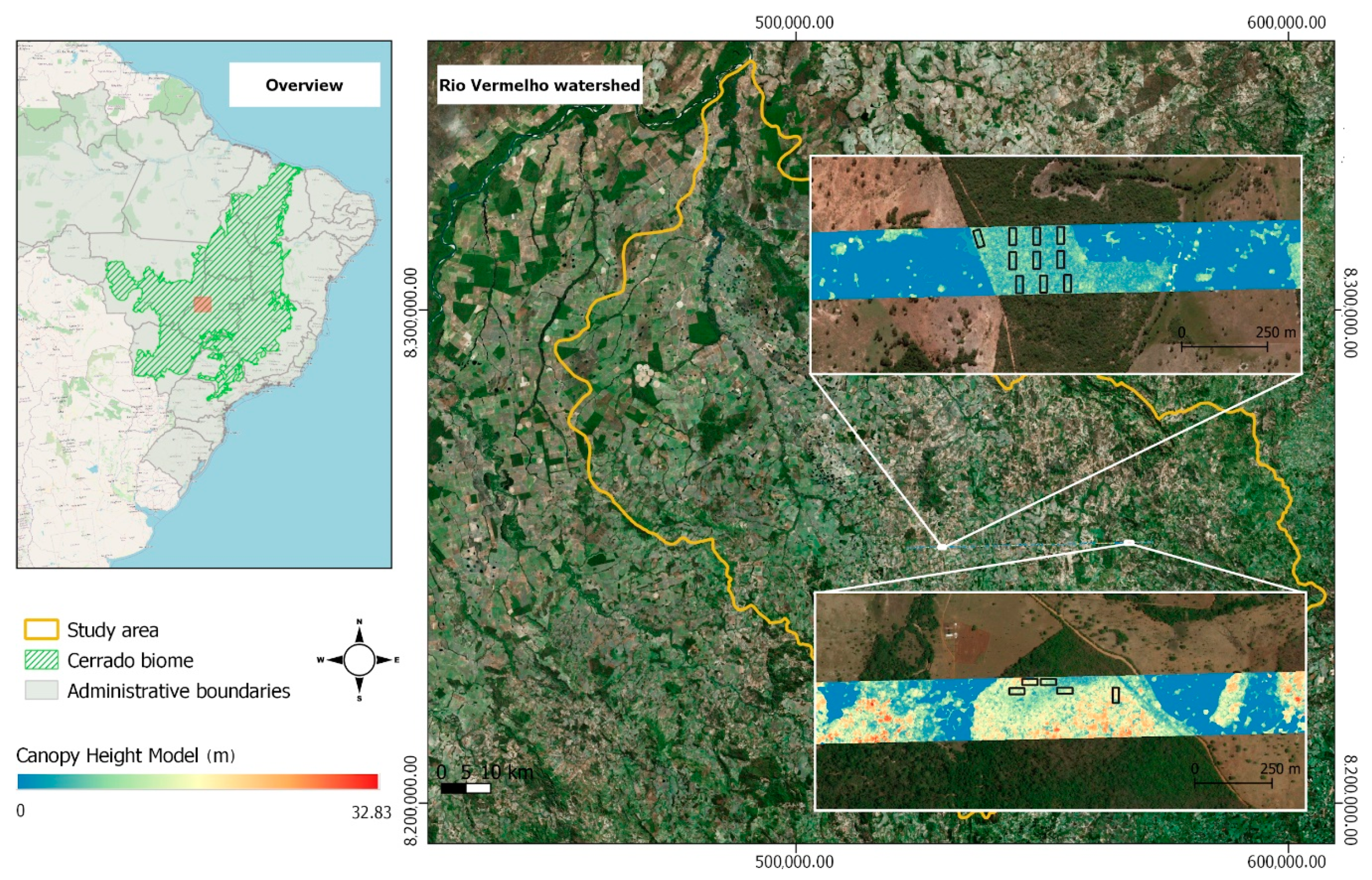
2.1. Study Area

The study site is located in the Rio Vermelho watershed, which is part of the Rio Araguaia watershed in the state of Goiás, Central Brazil (Figure 1), and it covers an area of 1,082,460 ha. The landscape topography is typically lowland, and the Cerrado biome’s climate is semi-humid (Aw in the Köppen’s climate classification system). It is a tropical savanna with two marked seasons: a dry winter (from May to September) and a rainy summer (from October to April). This watershed is characterised by a relatively constant air temperature throughout the year, with minimum and maximum temperatures of 20 °C and 32 °C, respectively) [57,58]. Intense and localised precipitation and frequent dry spells occur.

The Rio Vermelho watershed is part of a region in the Goiás State called “Mato Grosso Goiano”. This denomination is based on the historical extensive and dense native forest cover (typical for the Mato Grosso State) in the region [59]. This part of the Brazilian Cerrado underwent intensive human settlement in the 18th century due to the Brazilian gold rush in Central Brazil [60]. Since forests in the Cerrado are supposedly associated with soils with good fertility, most of the forest-covered areas have already been converted to other uses, mainly croplands and pastures [59], sometimes resulting in land degradation. Today, forest formations are restricted to a small and few fragments. Pastures cover more than 57% of the study area [6], and livestock ranching is the main economic activity in the region. By 2018, only approximately 33% of the native vegetation persisted [12,61], and the remaining native vegetation is fragmented [62] and often located in legal reserves areas.

Vegetation

Most of the Cerrado natural vegetation is comprised of savanna formations (cerrado stricto sensu). However, forest formations such as woodlands, riparian forests, and seasonal forests play an important role in the carbon balance, because they have a higher carbon stock density [63]. In the Rio Vermelho watershed, woodlands or cerradão (in Portuguese) and seasonal forest formations predominate as the forest remnants. The forest inventory sites were located in two fragments of cerradão, and the plots follow a structural and biomass gradient from: (a) a savanna-cerradão transition zone (lower biomass), (b) cerradão, and (c) cerradão-seasonal forest transition zone (higher biomass).

Dystrophic cerradão is typical for deep, highly lixiviated soil (Oxisols and sandy soils) areas with a seasonal tropical climate, and their canopy height varies between 8 and 15 m. Canopy cover varies between 50% and 90%, with an understory of shrubs and grass [62]. They are structurally similar to seasonal forests and differ mainly in species composition, as they are comprised of seasonal forest as well as wooded savanna species [62,64].

Seasonal forests are often associated with more fertile soils (mesotrophic and eutrophic soils) and present different levels of deciduousness during the dry season. The canopy height varies between 15 and 25 m, and the forest cover is between 70% and 95% during the rainy season. In the dry season, the canopy cover can be lower than 50% in seasonal semideciduous forests and lower than 35% in seasonal deciduous forests [62].

In wooded savannas, most trees are shorter and sparser than in forest formations, allowing for a continuous herbaceous grassy layer. Wooded savannas are separated into subgroups according to their structural gradient: cerrado ralo (2–3-m-tall trees with 5–20% canopy cover), cerrado sensu stricto or typical cerrado (3–6-m-tall trees with 20–50% forest cover), and cerrado denso (8–15-m-tall trees with 50–70% forest cover) [65].

2.2. Methodology

Figure 2 shows the flowchart of the methodology used to produce the AGB map of the Rio Vermelho watershed. Our reference datasets consisted of ground measurements and airborne LiDAR data. We used a combination of Earth Observation (EO) datasets from multispectral passive optical and synthetic aperture radar (SAR) sensors as predictor variables to estimate the AGB of the study area. The description of each step of the methodology is provided in the following subsections.

2.2.1. Ground Truth Data

We used woody AGB data from 15 (20 m × 50 m) field plots located in cerradão vegetation to estimate the AGB from airborne LiDAR. These plots were established in 2014, and all trees with a diameter at breast height (dbh) ≥ 5 cm at 1.30 m above the ground were considered. The tree heights were measured with a digital clinometer (HAGLOF ECII-D). The basal area in m² was calculated from the dbh (basal area = (π/4) ∗ (dbh/100)²) (

Table 1. Floristic and structural characterisations of the plots located in fragments of the native Cerrado vegetation in the Rio Vermelho watershed, Goiás State, Brazil. WS-FS = savanna-cerradão transition zone, TFS = cerradão, FS-SF = cerradão-seasonal forest transition zone; S = species richness, TD = tree density, DBH = diameter at breast height, H = height, TBA = tree basal area, AGB = aboveground biomass, and CV= coefficient of variation.

Plot ID	Vegetation Type	S (Species)	TD (Ind. ha−1)	DBH Range (cm) (Mean/CV%)	H (m) (Mean/CV%)	TBA (m2/ha)	AGB (Mg ha−1)
Itapirapuã 1	WS-FS	38	990	5.0–36.7 (9.1/56.9)	1.7–11.2 (5.8/26.9)	13.5	19.3
Itapirapuã 2	WS-FS	32	920	5.0–45.5 (9.5/54.7)	1.6–13.4 (5.6/35.5)	10.8	21.2
Itapirapuã 3	WS-FS	45	1030	5.0–29.4 (10.4/54.5)	2.1–14.0 (5.8/35.9)	15.0	24.5
Itapirapuã 4	WS-FS	41	1040	5.3–52.0 (9.8/58.4)	1.3–12.6 (5.5/33.4)	14.4	28.2
Itapirapuã 5	TFS	36	1140	5.0–41.4 (10.3/60.4)	2.0–12.8 (6.0/31.9)	16.4	32.2
Itapirapuã 6	TFS	45	1570	5.0–34.7 (10.5/47.0)	1.5–12.9 (6.5/31.6)	22.6	35.3
Itapirapuã 7	TFS	50	1990	5.0–43.7 (9.1/52.9)	1.8–13.2 (6.5/33.6)	21.9	36.8
Itapirapuã 8	TFS	60	1440	5.0–48.0 (10.4/61.2)	2.6–13.2 (6.1/31.8)	20.1	40.2
Itapirapuã 9	TFS	35	1210	5.0–53.3 (10.1/62.9)	1.8–13.1 (6.5/30.8)	17.0	40.9
Goiás 10	TFS	41	1260	5.0–35.3 (10.9/57.3)	3.6–19.6 (8.7/38.6)	20.5	52.8
Itapirapuã 11	TFS	39	1260	5.0–42.3 (11.2/65.9)	1.7–14.9 (6.3/36.3)	24.3	54.3
Goiás 12	FS-SF	38	1310	5.0–49.3 (11.3/61.5)	2.5–19.3 (9.3/33.3)	24.6	70.4
Goiás 13	FS-SF	26	690	5.0–49.0 (13.0/73.6)	3.4–22.0 (10.2/43.5)	18.3	77.0
Goiás 14	FS-SF	27	820	5.0–44.2 (13.2/63.5)	3.0–38.0 (12.5/48.7)	22.0	98.3
Goiás 15	FS-SF	24	760	5.0–41.7 (14.0/67.3)	2.5–26 (10.9/52.5)	24.4	103.9

). Ten plots were located in the remnants of native vegetation in the municipality of Itapirapuã (Figure 1, right panel, top zoom), while five plots were located in the municipality of Goiás (Figure 1, right panel, lower zoom).

As mentioned, the two native vegetation fragments sampled are classified as cerradão. However, due to the high structural heterogeneity in the Cerrado biome, there were considerable variations in the structure of the woody vegetation within the sampled plots. The floristic and structural characteristics of the plots described in Table 1 (and from Figure S1 to Figure S20 in the Supplementary Materials) corroborate that the sampled plots adequately represent the gradient of floristic-structural variation inherent to forest formations from all of the Cerrado. Thus, four plots were classified as a savanna-cerradão transition zone, seven as cerradão, and four as a cerradão-seasonal forest transition zone [62]. The sampled plots showed a height gradient directly related to the aboveground biomass stocks of woody vegetation. In the savanna-cerradão transition zone, the mean height was below 6 m, in the cerradão, between 6 and 8 m, and, in the cerradão-seasonal forest transition zone, above 9 m (Table 1). These plots were representative of the structural variation found in the cerradão vegetation of the region, with AGB values ranging from 19 to 104 Mg ha⁻¹ (Table 1).

In tropical ecosystems, species diversity is generally very high. Therefore, generalised (mixed-species) allometric models are more appropriate than species-specific equations [66,67]. We used the following mixed species allometric model [68] designed for cerradão (N = 87, R² = 0.94, residual standard error (RSE) = 0.13 Mg; RSE (%) = 49.83). The model estimates the woody AGB (only live trees were used) with a diameter at breast height ≥ 5 cm, excluding leaf biomass.

AGB = exp [−12.29 + 2.69 ∗ ln(dbh) + 0.80 ∗ ln(h)]

(1)

where dbh is the diameter at breast height, and h is height.

In our study, these in situ woody AGB estimates were then used to establish an empirical model to estimate AGB as a function of the structural metrics derived from the airborne LiDAR.

2.2.2. LiDAR Data

We used 60 tiles of airborne LiDAR data (covering a total area of 1009.01 ha) collected by the Sustainable Landscapes project led by the Brazilian Enterprise for Agricultural Research Corporation (EMBRAPA). The LiDAR data covered the municipalities of Itapirapuã and Goiás, Goiás State, Brazil. The flights took place between 20 June 2015 and 7 July 2015. The LiDAR dataset has an average density of returns of ~45 ppm² (points per square meter). The average altitude of the flights was ~850 m, with a field of view of 12°. Two LiDAR sensors (Optech Orion M300 and Optech ALTM 09SEN243) were used in these campaigns, but the percentage of flight line overlaps was high (~65%). LiDAR returns of all 15 plots are shown from Figure S6 to Figure S20 in the Supplementary Materials.

The LASTools software [69] was used to process the LiDAR data and to generate the following variables derived from the LiDAR point cloud data: DSM (digital surface model), CHM (canopy height model), DTM (digital terrain model), CC (canopy cover coverage), CD (canopy density), Max-H (maximum height), Percentile_p15, Percentile_p10, Percentile_p20, Percentile_p30, Percentile_p35, Percentile_p55, Percentile_p40, Percentile_p45, Percentile_p50, Percentile_p60, and Percentile_p65. Highly correlated variables were excluded, and the ones containing the most unique information, CHM, CC, and CD, were used to establish statistical models to extrapolate the spatially limited LiDAR AGB estimates to both the optical and radar observations (Figure 2).

2.2.3. Optical Data

The United States Geological Survey (USGS) Landsat 8 Collection 1 Tier 1 data consists of surface reflectance products generated from the Landsat 8 Operational Land Imager (OLI), with 30-m spatial resolution. The USGS atmospherically corrects the scenes using the Landsat 8 Surface Reflectance Code (LaSRC), which also uses the C function of the mask (CFMASK) algorithm [70] to generate a cloud, shadow, water, and snow mask. We selected all the scenes acquired in the period of 2015–2017 (244 scenes) to generate a cloud and shadow-free median temporal composite (Figure 2). In addition to the spectral bands, we generated a range of vegetation indices that could potentially be representative for the vegetation canopy structure, seasonality, and a measure of vegetation greenness. These were the normalised difference vegetation index (NDVI), normalised burn ratio (NBR), normalised difference moisture index (NDMI), and the soil adjusted vegetation index (SAVI). These indices have previously been used in similar studies [21,23,71,72,73].

2.2.4. SAR Data

We used the global 25-m resolution ALOS PALSAR/PALSAR−2 annual mosaics, which are freely available at https://www.eorc.jaxa.jp/ALOS/en/palsar_fnf/fnf_index.htm. This dataset was pre-processed by the Japanese Aerospace Exploration Agency (JAXA) using L-band SAR images of the backscattering coefficient acquired by the Advanced Land Observing Satellite (ALOS) and Advanced Land Observing Satellite-2 (ALOS-2). The mosaics consist of 10 × 10-degree tiles pre-processed to correct for geometric distortions (ortho-rectification) and topographic effects [74]. The mosaics were calibrated to γ0 using the following equation:

$${\gamma }^0=10xlo{g}_{10}{\left(DN\right)}^2+CF$$

(2)

where γ⁰ is the gamma-naught in decibels (dB), DN is the digital number in unsigned 16 bit, and CF is a calibration constant of 83.0 dB.

We reduced the noise of the mosaics by applying a temporal multi-channel filter [75] with a 5 × 5-pixel moving average window. Then, we applied a temporal normalisation between PALSAR and PALSAR-2 images aiming to correct for soil moisture and sensor differences. For our final PALSAR-2 composite, we used the median value of the three mosaics (2015, 2016, and 2017) (Figure 2). We observed a geolocation error of ~80 m on average for the PALSAR-2 mosaics in comparison to HR (high-resolution) imagery and Landsat 8 scenes. We generated a Sentinel-1 SAR median γ⁰ composite using 283 scenes from between 2016 and 2018, and we used this not as an input for our modelling but as a geolocation reference image. The PALSAR-2 composite was georeferenced against the Sentinel-1 composite using a SAR-to-SAR co-registration. This approach, instead of a SAR-to-optical approach, was chosen to avoid errors derived from the different viewing geometries of SAR and optical images. The variables used for this study were the SAR backscatter coefficients (${\gamma }_{HV}^0$ and ${\gamma }_{HH}^0$) and two SAR indices—namely, the radar forest degradation index (RFDI) and the cross-polarised ratio (CpR) [74].

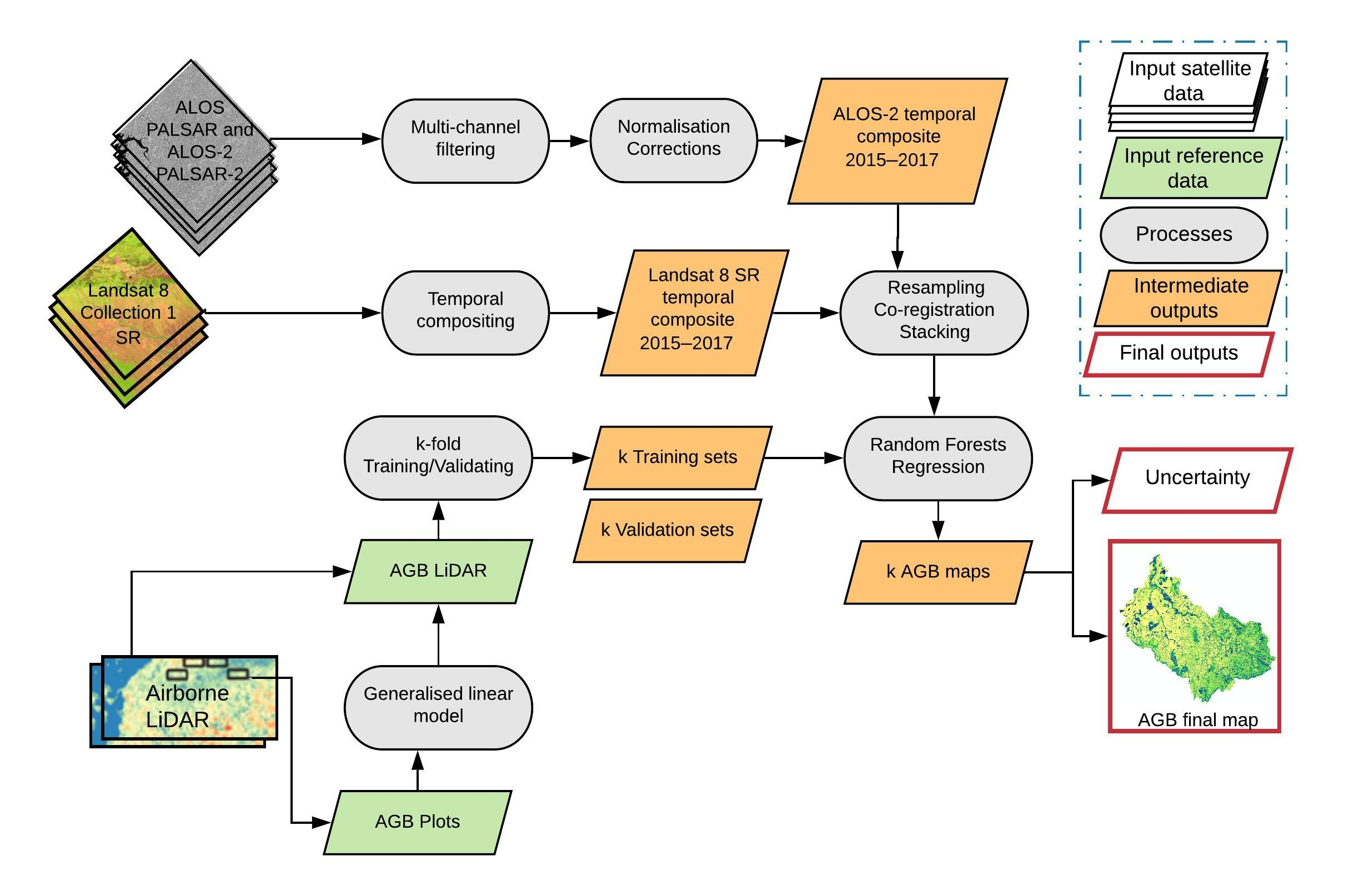
2.3. Modelling Framework

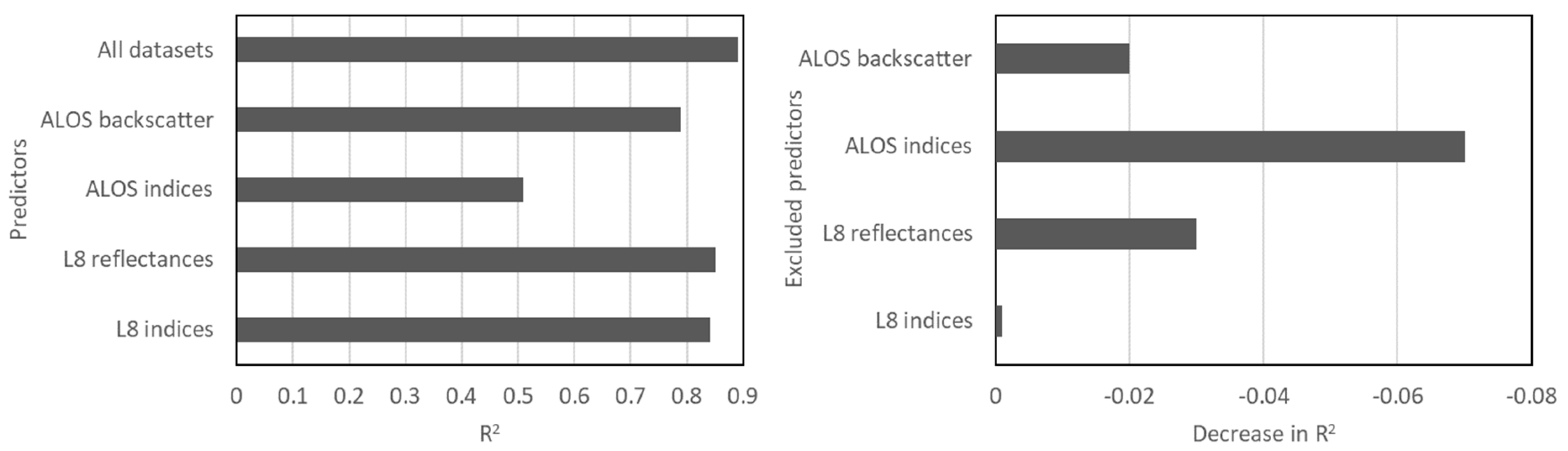
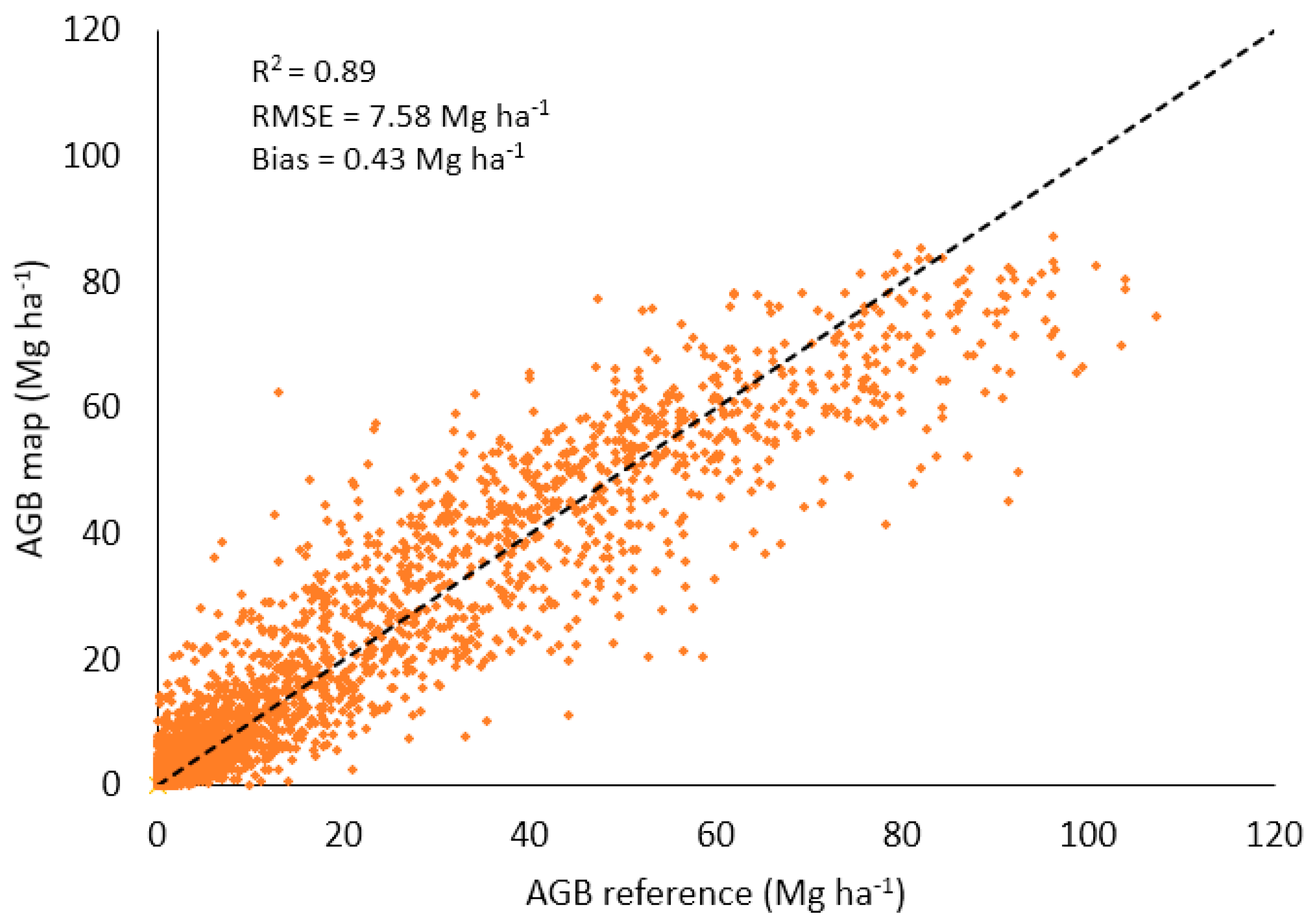
We adopted a two-stage upscaling method from field measurements to airborne LiDAR point clouds and from the LiDAR-based estimates to satellite imagery. We estimated the woody AGB of the field plots and used these as a reference to estimate the woody AGB across the LiDAR footprints using LiDAR-derived structural variables as a predictor. Our field plots covered a representative range of flora and structure of the woody vegetation (Table 1) from 19 Mg ha⁻¹ to 104 Mg ha⁻¹. As the LiDAR point clouds are sensitive to the forest structure, we assumed that these plots could express the physical and structural variations of the vegetation of the study site, and we allowed the AGB LiDAR model to extrapolate for values < 19 Mg ha⁻¹. This field-to-LiDAR procedure allowed us to increase our sampling from the 15 plots to thousands of observations derived from the LiDAR footprint covering a wide range of woody AGB and vegetation types. We then used these LiDAR AGB, representative for the vegetation in the region, in combination with EO datasets to estimate the woody AGB over the entire Rio Vermelho watershed.

The first step was to model the relationship between LiDAR woody vegetation structural variables and the AGB estimated from the field plots (Figure 2). We generated raster-based LiDAR vegetation structural variables with using a 1-m pixel size. We then used the average value of the pixels within the 20 × 50-m plots (0.10 ha) to develop our models. As we had a limited number of field plots, we had to limit the number of variables included in the empirical models as well. Based on a visual exploration of the relationships between the dependent and independent variables, as well as the distribution of each predictor, we identified three potential predictors: canopy height model (CHM), canopy density (CD), and canopy cover (CC). We then used all possible combinations of these variables to find the best generalised linear model to estimate the AGB based on the Akaike’s information criterion corrected for a small sample size (AICc). This final model was used to estimate the AGB over the entire LiDAR footprint at a 30-m spatial resolution (0.09 ha). The next step was to model the relationship between the estimated LiDAR AGB and the EO datasets. These EO datasets were resampled, co-registered, and stacked at 30-m spatial resolutions (Figure 2). We used the LiDAR AGB pixels (N = 2,973) as training and test samples in a regression version of the random forest (RF) algorithm [76] in the Google Earth Engine [77], which was implemented within a k-fold cross-validation framework [73]. The following variables were used as predictors in the model: ${\gamma }_{HV}^0$; ${\gamma }_{HH}^0$; RFDI; CpR from the PALSAR-2 data; and blue, green, red, near infrared, and shortwave infrared bands, as well as NDVI, NBR, NBR2, NDMI, and SAVI from the Landsat 8 data. RF is a nonparametric machine-learning algorithm that uses a bootstrap technique to construct multiple decision trees. Jackknife tests were also run to compare the importance of the predictor variables based on a R² of the model. Due to the randomness (stochastic nature) of the RF algorithm, the importance may change for each run. Thus, the variable importance analysis was run for each k and then averaged to produce the overall importance figures. The test was performed running each single set of variables in isolation to assess the accuracy of each set. The higher the R², the higher the importance of the variable. Then, a set of variables was excluded each time from the whole set to assess the drop in the variance explained by the model.

The k-fold cross-validation framework was used to train and validate the algorithm (Figure 2), maximising the reference data available. Figure 2 shows the overview of the method used to produce the AGB map and the uncertainty characterisation in the Rio Vermelho watershed. The whole reference dataset was used for both training and validation purposes. The dataset was stratified by three AGB levels (low, medium, and high), and randomly sampled into the folds to ensure that all folds have similar probability distribution functions of the AGB. Then, k-1 folds were used to train the RF algorithm and to produce the AGB map, while the remaining fold was used for the validation. The process was then run k times, reusing the folds for training purposes but using them only once for validation purposes. The final outputs were k AGB maps over the study area. The mean value of the k AGB maps was used as the final AGB map, and we used the standard deviation (SD) of the k estimates for any given pixel to generate a prediction error (${\mathsf{\sigma }}_{prediction}$) map. This error also accounts for the representativeness of the sampling sites of the true distribution of AGB in the region [21]. The total SD (${\mathsf{\sigma }}_{AGB}$) was propagated, as explained in Rodriguez-Veiga et al. [29] and Saatchi et al. [21], as follows:

$${\mathsf{\sigma }}_{AGB}={\left({\mathsf{\sigma }}_{measurement}^2+{\mathsf{\sigma }}_{LiDAR}^2+{\mathsf{\sigma }}_{allometry}^2+{\mathsf{\sigma }}_{sampling}^2+{\mathsf{\sigma }}_{prediction}^2\right)}^{\frac{1}{2}}$$

(3)

where the measurement error (${\mathsf{\sigma }}_{measurement}$) of the tree level parameters averaged at the plot scale was assumed as 10% [78], the LiDAR error (${\mathsf{\sigma }}_{LiDAR}$) was assumed as 1.5% (from a 0.11-m instrument error for an average 7.13 m canopy height), the allometric error (${\mathsf{\sigma }}_{allometry}$) was assumed to be 49.83% (Scolforo et al. [68]), and the sampling error (${\mathsf{\sigma }}_{sampling}$) from the variability of AGB within the pixels was estimated as 12.39% based on Réjou-Méchain et al. [79].

Our k-fold cross-validation assessment followed James et al. [80] and involved the calculation of the R², RMSE, rel. RMSE, and the mean bias error (MBE). Aside from the overall assessment, we also analysed the errors by biomass ranges. Finally, we also compared our AGB estimates to four other studies [21,22,23,81] (

Table 2. Summary of forest aboveground biomass (AGB) maps used for comparison with our study results. RMSE: root mean square error, rel. RMSE: relative root mean square error.

Study	Coverage	Year	Spatial Resolution	Methodology	Accuracy/Uncertainty
Saatchi et al. [21]	Pantropical	early 2000s	1 km	MaxEnt (field measurements, GLAS data, optical and microwave imagery)	Uncertainty from ±6% to ±53%
Baccini et al. [23]	Pantropical	2007–2008	500 m	Random Forest algorithm (field data, GLAS and MODIS data)	RMSE = 25 Mg C/ha for tropical America
Avitabile et al. [22]	Pantropical	2000–2008	1 km	Weighted linear averaging method (biomass reference datasets, Saatchi et al. [21] map and Baccini et al. [23] map)	RMSE = 87~98 Mg/ha; Mean error: almost null in most cases
Santoro et al. [81]	Global	2010	100 m	Water Cloud Model (ALOS PALSAR, Envisat, Landsat and field plots)	rel. RMSE = 57.1% and Bias = 10.6 Mg ha −1 for tropical areas

). Baccini et al. [23] used multi-sensor satellite data to estimate the aboveground live woody vegetation carbon density for pantropical ecosystems with a 500-m resolution. Saatchi et al. [21] mapped the total carbon stock in live biomasses (above- and belowground) in the tropics using a combination of data from in situ inventory plots and satellite LiDAR samples of the forest structure to estimate the carbon storage, plus optical and microwave imagery (1 km resolution), to extrapolate over the landscape. Santoro et al. [81] estimated AGB globally at a 100-m resolution by combining spaceborne SAR, LiDAR, and optical observations for the year 2010, with auxiliary datasets from forest inventories—namely, additional remote-sensing observations, climatological variables, and ecosystems classifications. Avitabile et al. [22] combined two existing datasets of vegetation aboveground biomasses (AGB) into a pantropical AGB map at a 1-km resolution using an independent reference dataset of field observations and locally calibrated it using high-resolution, harmonised, and upscaled biomass maps. For the comparison of our results to these maps, we aggregated all of them to the same spatial resolution (1 km).

3. Results

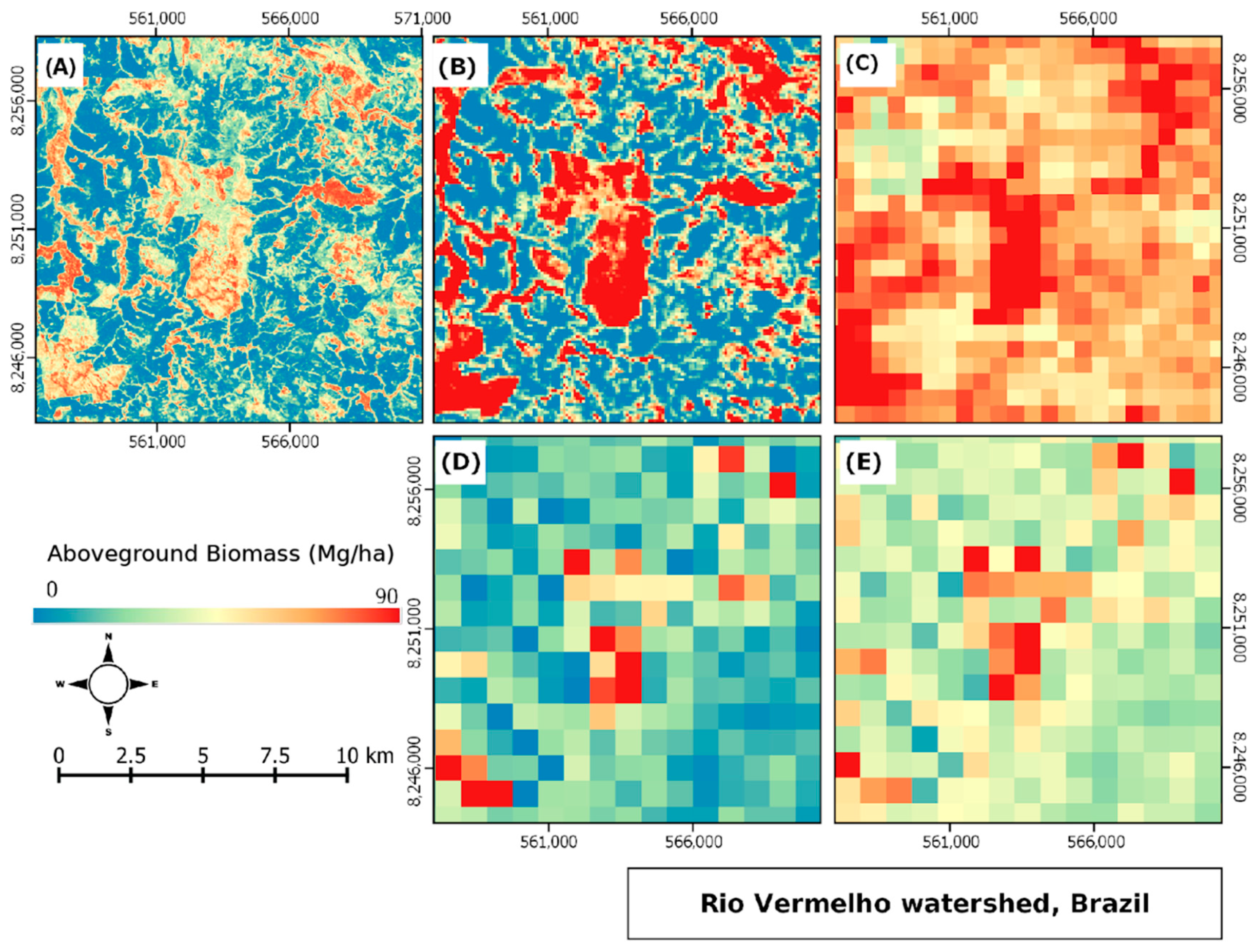
3.1. LiDAR-Derived AGB Map

Table 3. Model comparison according to Akaike’s information criterion corrected for a small sample size (AICc). Parameters for each model include: LogLik (log-likelihood), k (number of predictor variables), AICc (Akaike’s information criterion corrected for a small sample size), ΔAICc (difference in AICc between the current and the best model), Adj R² (adjusted coefficient of determination), and RMSE (root mean square error). The intercept and coefficients, as well as the coefficient of determination (R²) for each model, are also presented. CHM = canopy height model, CD = canopy density, and CC = canopy cover.

Model	LogLik	k	AICc	ΔAICc	Adj R2	RMSE (Mg ha−1)
AGB = −61.92 + 4.88*CHM + 0.83*CC	−49.90	2	107.81	0.00	0.93	6.74
AGB = −107.18 + 2.21*CC − 1.26*CD + 6.34*CHM	−49.40	3	108.81	1.00	0.93	6.52
AGB = −30.03 + 4.30*CHM + 0.66*CD	−50.56	2	109.13	1.32	0.92	7.04
AGB = 2.44 + 6.25*CHM	−52.71	1	111.42	3.61	0.89	8.12
AGB = −27.17 − 2.31*CC + 3.22*CD	−54.83	2	117.66	9.85	0.86	9.36
AGB = −76.56 + 1.76*CD	−56.56	1	119.13	11.32	0.81	10.51
AGB = −173.08 + 2.48*CC	−60.72	1	127.44	19.63	0.69	13.86
AGB = 52.34	−69.39	0	142.78	34.97	0.00	24.70

shows the models tested in this study. The AGB = f(CHM, CC) model was the one that best explained the field-based AGB variations (Table 3, adj R² = 0.93, RMSE = 6.74 Mg ha⁻¹, or 13% of the mean biomass values) and, therefore, was used to predict the AGB over the whole LiDAR flight footprint. This predicted LiDAR AGB was used to generate training and test samples to run the RF algorithm to extrapolate the AGB to the EO datasets covering the entire Rio Vermelho watershed. Although the AGB = f(CC, CD, CHM) model resulted in a slightly smaller RMSE and a higher AIC than AGB = f(CHM, CC), both models showed the same R² (= 0.93) and RMSE (6.74 Mg ha⁻¹ or rel. RMSE = 13%). We therefore opted for the AGB = f(CHM, CC) model, as it is more parsimonious and only uses two independent variables (Table 3 and Figure S1 in the Supplementary Materials).

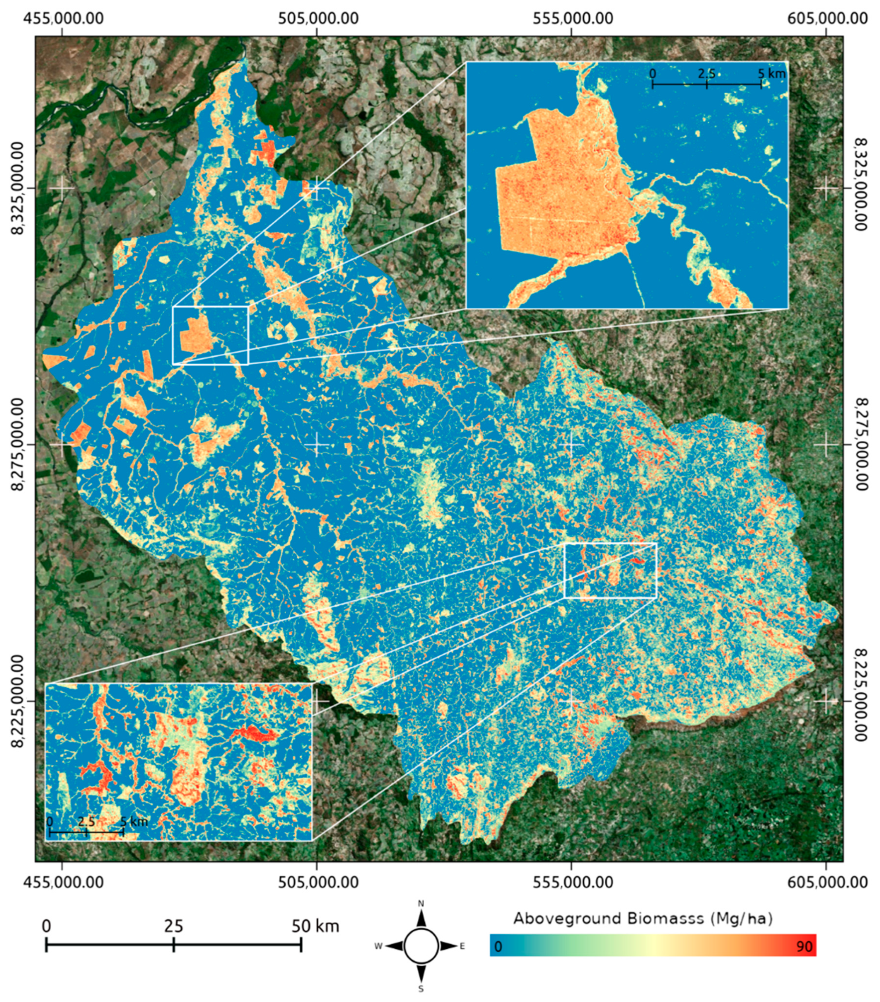
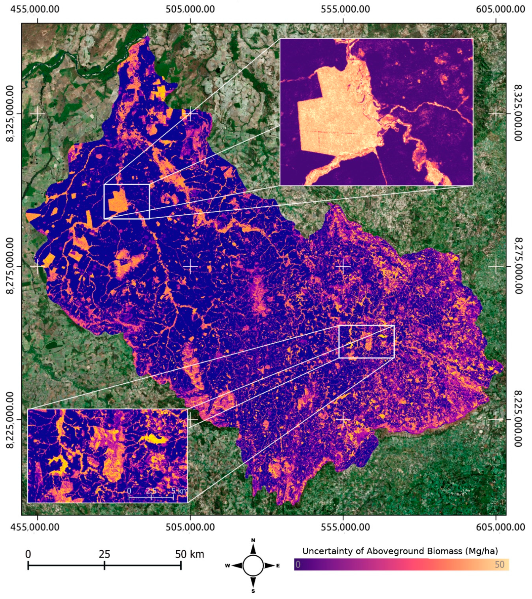
3.2. AGB and Uncertainty Map

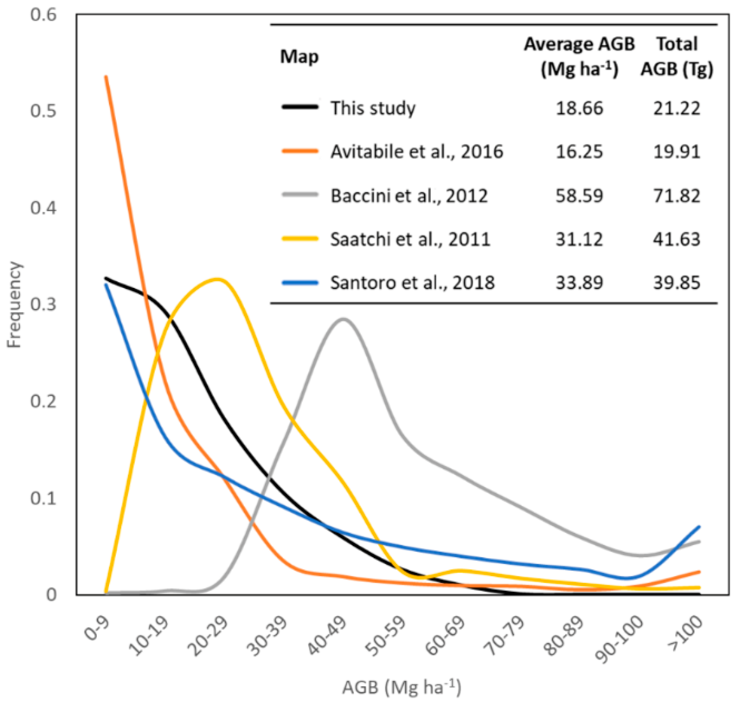
The AGB varied from 0 to 90 Mg ha⁻¹ per pixel (Figure 3), whereas the pixel-scale uncertainty estimated by the error propagation approach ranged from 0 to 49 Mg ha⁻¹ (Figure 4). Figure 5 shows the averaged variable importance analysis across the k-fold procedure for each set of variables derived from Landsat 8 (L8) and ALOS-2/PALSAR-2 (ALOS) included in the random forest (RF) model. These results indicated that the Landsat reflectances composite was the most important set of variables when predicting AGB. However, the ALOS indices contain more unique information not represented by the other variables, as shown by the largest decrease in accuracy when the variable was excluded. Figure 6 shows the overall accuracy assessment and

Table 4. Cross-validation assessment by the AGB range. MBE: mean bias error.

AGB Range (Mg ha−1)		Number of Pixels	Reference AGB (Mg ha−1)	Map AGB (Mg ha−1)	MBE (Mg ha−1)	RMSE (Mg ha−1)	Rel. RMSE
0–20	2084		4.4	5.7	1.3	4.8	109%
20–40	379		29.5	31.8	2.3	10.4	35%
40–60	287		49.3	48.8	−0.5	10.8	22%
60–80	152		69.2	62.6	−6.6	11.4	16%
>80	71		89.2	72.3	−17.0	20.0	22%

the assessment by AGB range.

The accuracy assessment between the AGB map predicted from EO and the AGB reference from LiDAR showed R² = 0.89, RMSE = 7.58 Mg ha⁻¹, rel. RMSE = 43%, and bias = 0.43 Mg ha⁻¹ (Figure 6). Our map shows an underestimation of very high AGB (negative bias) and a slight overestimation of low AGB (positive bias) [28] (Table 4). We also found a RMSE of 6.39 Mg ha⁻¹ (rel. RMSE = 61%) for AGB lower than 50 Mg ha⁻¹ and a RMSE = 13.41 Mg ha⁻¹ (rel. RMSE = 19%) for AGB higher than 50 Mg ha⁻¹. Details of the accuracy assessment by biomass range are shown in Table 4.

Figure 7 and Figure 8 show the comparisons between the AGB estimates produced in our study and four other studies [21,22,23,81]. Although these maps were estimated using different methods and at different resolutions over the pantropical area, it is interesting to observe how the different data products compared to each other. While this study and Avitabile et al. [22] presented probability distribution functions skewed towards low biomass ranges, other studies [21,23,81] showed distributions tending towards much higher AGB levels, with averages two to three times larger than those found in this study and by Avitabile et al. [22] (Figure 7). Figure 8 shows that the datasets from [21,23,81] did not adequately represent all the variations that exist in the area due to the lower spatial resolution and, also, generally showed a greater overestimation of the AGB. Although Santoro et al. [81] provided more details in terms of the distribution of AGB in comparison with the other three maps, their map still overestimated the AGB compared to our results. In the map developed in this study, one can observe the AGB variation in detail, which is corroborated by the observed high coefficient of determination (R² = 0.89) between the AGB reference datasets and the final AGB map.

4. Discussion

In 2014, Brazil submitted a greenhouse gas (GHG) emission report (Forest Reference Emission Level (FREL) for Reducing Emissions from Deforestation for REDD+ under the United Nations Framework Convention on Climate Change (UNFCCC)) [82] as part of the country’s commitment to reduce GHG emissions from deforestation in the Amazon (FREL Amazonia). Brazil indicated in that report that its national report would be the sum of the FRELs for each of the six Brazilian biomes. The FREL report for the Cerrado biome (FREL Cerrado), together with the FREL Amazonia, showed that emissions induced by land use changes accounted for approximately 73% of the emissions in Brazilian territory [82]. This shows the importance of the Cerrado biome for REDD+ policies and for the efforts of climate change mitigation in the country, such as the national inventories initiatives as part of the Third National Communication of Brazil to the UNFCCC [63].

The reduced number of studies on the quantification and spatial variability of the total Cerrado AGB stocks limits a full understanding of CO₂ emission patterns in this biome. These are especially critical for local and national climate governance strategies. Appropriate management and mitigation models will depend on the accuracy of this information. We produced the first high-resolution continuous map of AGB in an area of the Brazilian Cerrado, making use of a combination of vegetation inventory plots, airborne light detection and ranging (LiDAR) data, and satellite images (Landsat 8 and ALOS-2/PALSAR-2). Fieldwork in the Brazilian Cerrado is challenging, time-consuming, and expensive, and existing field datasets still do not entirely represent the extent of the biome. An alternative to increasing the sample size is using LiDAR by upscaling the information from field plots (which ideally should be representative of the analysed ecosystem). This strategy has been used in recent studies in other forest types [83,84]. We increased our sample size thousands of times, reaching a very high R² of 0.93 in the AGB LiDAR estimation. This consistent result was essential to allow us to use LiDAR as a reference for our AGB modelling process using satellite images and machine learning.

In our study, the RF algorithm proved to be a good strategy to estimate the AGB in the study area (Table 4 and Figure 6). This result can be attributed to the ability of these techniques to capture the nonlinearity present in the data, as they can approximate complex functions [85]. This is an important characteristic for the modelling of vegetation, such as ecological patterns governed by nonlinear and interactive processes at any ecological scale [85], since they usually present complex behaviours [28].

Current sources of AGB information for the Cerrado are the global and pantropical maps that have a limited spatial resolution (from 100 m to 1 km) and questionable high estimations for this biome (Figure 7 and Figure 8) [2]. Figure 7 shows the distribution by AGB intervals, average, and total AGB observed from our study and the four global and pantropical maps over the Rio Vermelho watershed [21,22,23,81]. This study and the one conducted by Avitabile et al. [22] presented distributions with an average of 18.66 Mg ha⁻¹ and 16.25 Mg ha⁻¹, respectively. On the other hand, Santoro et al. [81], Saatchi et al. [21], and Baccini et al. [23] showed distributions tending towards much higher AGB levels, with averages of 33.89 Mg ha ⁻¹, 31.12 Mg ha ⁻¹, and 58.59 Mg ha ⁻¹, respectively. Saatchi et al. [21] and Baccini et al. [23] found the distributions of the AGB tending toward a normal distribution for the study site, which was not the case for the map produced by Avitabile et al. [22], Santoro et al. [81], and our study. Morandi et al. [2] recently calculated AGB values for the Cerrado biome using a large independent dataset of field plots. The study estimated an average of 20.4 ± 6.0 Mg ha⁻¹ for the central areas of the Cerrado biome, where this watershed is located, which agrees with our study results. However, global and pantropical studies showed significantly higher AGB levels in comparison to Morandi et al. [2], our study (Figure 7), and to the AGB values measured in our field plots. We also observed the tendency of these products to overestimate the AGB on the lower AGB ranges, which results from the models attempting to compensate for the underestimation at the higher AGB ranges due to the potential signal saturation [28]. This agrees with previous studies that have indicated the inconsistency of these products when compared in several forest biomes [86,87]. Our regional AGB map (Figure 3) takes the local vegetation structure of the Brazilian Cerrado into account and has a spatial resolution of 30 m. Overall, the relationship between our reference data and the remote-sensing variables is relatively high (R² = 0.89), with a root mean square error (RMSE) of 7.58 Mg ha⁻¹. The accuracy assessment showed that our map underestimates high AGB levels and slightly overestimates low AGB levels (Table 4). This result fully meets the biomass product accuracy requirements set by the BIOMASS mission (RMSE < 10 Mg ha⁻¹ for AGB < 50 Mg ha⁻¹ and rel. RMSE < 20% for AGB > 50 Mg ha⁻¹) [56], with a RMSE of 6.39 Mg ha⁻¹ for AGB < 50 Mg ha⁻¹ and a rel. RMSE = 19% for values > 50 Mg ha⁻¹. It is important to highlight that we were interested in a representative range for cerradão AGB, including transitions to other vegetation types.

When analysing the statistical indicators of the goodness-of-fit (RMSE and R²) (Table 4) using the RF technique, a higher accuracy was achieved for the AGB range > 40 Mg ha⁻¹. However, even though we are confident in our AGB estimations, we have to be cautious with the estimations of AGB values < 19 Mg ha⁻¹, areas that are not covered by woody vegetation (e.g. grasslands, agriculture, and bare soil), as our field-to-LiDAR AGB model was developed using field plots located only in woody vegetation areas. In Figure 6, we can observe an underestimation of the highest AGB ranges (AGB > 80 Mg ha⁻¹), which is also reflected in the negative bias for this high AGB level (Table 4). The range of predictions random forest regression can make is bound by the highest and lowest values in the training data. This can lead to overestimations in the lower value range and underestimations in the higher range [88]. The scatterplot between the satellite AGB estimates from our results and the LiDAR AGB showed this effect with the slight underestimation of high AGB (Table 4 and Figure 6). This effect was also observed in the studies of Nunes and Görgens [88] and Zhang and Lu [89].

It is reported that machine-learning techniques can provide more accurate estimates than classical regression models [88]. Silva et al. [90] evaluated the use of machine-learning techniques and mixed models to estimate the volume and AGB of individual trees in the Brazilian Cerrado. The machine-learning techniques presented, and mixed-effect models, showed similar and highly accurate results (R² = from 0.97 to 0.99 and RMSE = from 12% to 13%) [58]. According to Silva et al. [90], because the modelling of forest resources commonly presents complex relationships among the variables, nonlinear mixed-effects modelling (NLME) and machine-learning techniques such as RF, adaptive network-based fuzzy inference systems (ANFIS), and artificial neural networks (ANNs) may be good alternative modelling techniques. In our study, using RF, we produced an AGB map of an area in the Brazilian Cerrado with a R² of 0.89 and RMSE of 7.58 Mg ha⁻¹. Previous studies tried to estimate the AGB in savannas using satellite data and reached performances lower than the results from our work [54,91,92].

Over the last decades, several studies have used SAR, especially ALOS PALSAR L-band radar images, to estimate the AGB of tropical savannas. Mermoz et al. [93] used ALOS PALSAR data to map the AGB in savanna ecosystems in Cameroon. They argued that L-band PALSAR mosaics are suitable for the retrieval of savanna AGB (typically less than 100 Mg ha⁻¹) at the national and continental scales. In a similar study, Carreiras et al. [27] tested a combination of field data and ALOS PALSAR backscatter intensity to reduce the uncertainty in the estimation of vegetation AGB in the Miombo savanna woodlands of Mozambique (East Africa). They applied a machine-learning algorithm, resulting in a good fit and accurate model (R² = 0.95 and RMSE = 5.03 Mg ha⁻¹). However, since they used bootstrap samples in combination with a cross-validation procedure, the reported cross-validation statistics could be overoptimistic [22]. A combination of datasets from different sources, such as in this study, proved to be efficient when the goal was to reduce uncertainties in the AGB estimates. Recent studies have explored the combination of different data types. Braun et al. [91] used passive and active microwaves to estimate the AGB of savannas. They introduced the integration of passive brightness temperature as an additional variable for AGB estimation, based on the hypothesis that it contains information complementary to the microwave backscatter coefficient from active sensors.

As we found in our work, many studies have shown the advantages of combining optical and SAR datasets using machine-learning techniques such as RF for AGB estimations. The optical data are sensitive to the biophysical properties of the vegetation, and radar data are more sensitive to the electrical and geometrical information of the vegetation—more specifically, the moisture content and vegetation structure. Forkuor et al. [46] showed in a recent study that combining field inventory data with Sentinel 1 (SAR) and Sentinel 2 (optical) to estimate the AGB in the West African dryland forest (tropical savanna and woodlands) using a RF algorithm performed much better than either one of them alone, reaching a R² of 0.90. This corroborates our results, which have also shown an improvement in accuracy using the combination of SAR and optical datasets rather than using either one individually. Our study also showed the highest performance (R² = 0.89) when all variables were included. The variable importance analysis (Figure 5) showed a slightly superior R² for Landsat 8 reflectance data (R² = 0.84) in comparison to ALOS−2 backscatter data (R² = 0.79) when mapping the AGB using a single set of data. Landsat 8 indices seem to have an almost identical performance to the Landsat 8 reflectance data, and there is no significant drop in performance when the indices are excluded (Figure 6). Conversely, the exclusion of the ALOS indices from the whole set results in the largest drop of R² (i.e., −0.07), despite having the lowest performance when used alone (R² = 0.51). This agrees with previous studies that found a higher contribution of the optical reflectance data to estimate AGB, potentially due to the sensitivity of optical data to shadow and moisture [23,29,94], which can be a key factor in sparse vegetation such as Cerrado. Additionally, the relatively low AGB levels in the study area might provide a level playing field with L-band SAR data, which usually presents a sensitivity of the signal to higher AGB levels than optical data [95,96,97,98,99]. Our study highlighted the need to use remote sensing in combination with local vegetation inventories to effectively quantify the spatial variation of AGB in ecosystems of the Brazilian Cerrado. Future high-resolution maps of ABG will likely be more useful to quantify carbon emissions from Cerrado degradations at the local and regional scales. The methodology presented here has the potential to be used to generate the first of its kind AGB map of the entire Brazilian Cerrado, which is often neglected in carbon stock assessments of the South American continent.

5. Conclusions

We provided the first high-resolution map of the AGB (30-m resolution) of a Brazilian Cerrado area using a combination of field inventory plots, airborne light detection and ranging (LiDAR) data, and satellite images (Landsat 8 and ALOS−2/PALSAR−2). We used random forest (RF) models and jackknife analyses to study the importance of remote-sensing variables to quantify the AGB of cerradão at large scales. Overall, the relationship between the reference data and remote-sensing variables is strong (R² = 0.89), with a root mean square error (RMSE) of 7.58 Mg ha⁻¹. Spatially, our map slightly underestimated and overestimated the values of the AGB in few areas of the savanna (bias = 0.43 Mg ha⁻¹). However, this spatial bias is similar to other AGB maps. Our study highlights the need to use remote sensing in combination with local field inventories to effectively quantify the spatial variation of AGB in the ecosystems of the Brazilian Savanna.

References

1. Instituto Brasileiro de Geografia e Estatistica (IBGE). Biomas E Sistema Costeiro-Marinho do Brasil. 2019. Available online: https://www.ibge.gov.br/apps/biomas/ (accessed on 18 August 2020).
2. Morandi, P.S.; Marimon, B.S.; Marimon-Júnior, B.H.; Ratter, J.A.; Feldpausch, T.R.; Colli, G.R.; Munhoz, C.B.R.; Júnior, M.C.D.S.; Lima, E.D.S.; Haidar, R.F.; et al. Tree diversity and above-ground biomass in the South America Cerrado biome and their conservation implications. Biodivers. Conserv. 2018, 29, 1519–1536. [Google Scholar] [CrossRef] [Green Version]
3. Klink, C.A.; Machado, R.B. Conservation of the Brazilian Cerrado. Conserv. Boil. 2005, 19, 707–713. [Google Scholar] [CrossRef]
4. Sano, E.E.; Rodrigues, A.A.; Martins, É.S.; Bettiol, G.M.; Bustamante, M.M.; Bezerra, A.S.; Couto, A.F.; Vasconcelos, V.; Schüler, J.; Bolfe, E.L. Cerrado ecoregions: A spatial framework to assess and prioritize Brazilian savanna environmental diversity for conservation. J. Environ. Manag. 2019, 232, 818–828. [Google Scholar] [CrossRef] [PubMed]
5. Ribeiro, S.C.; Fehrmann, L.; Soares, C.P.B.; Jacovine, L.A.G.; Kleinn, C.; Gaspar, R.D.O. Above- and belowground biomass in a Brazilian Cerrado. For. Ecol. Manag. 2011, 262, 491–499. [Google Scholar] [CrossRef]
6. Coutinho, L.M. O conceito de cerrado. Rev. Bras. Bot. 1978, 1, 17–23. [Google Scholar]
7. Delitti, W.B.C.; Meguro, M.; Pausas, J.G. Biomass and mineralmass estimates in a "cerrado" ecosystem. Braz. J. Bot. 2006, 29, 531–540. [Google Scholar] [CrossRef]
8. Brazil. Agricultural Development Plan Matopiba, Law no. 8.447–05/06/2015. 2015. Available online: http://www.planalto.gov.br/ccivil_03/_ato2015-2018/2015/decreto/d8447.htm (accessed on 20 December 2019).
9. Spera, S.A.; Galford, G.L.; Coe, M.T.; Macedo, M.N.; Mustard, J.F. Land-use change affects water recycling in Brazil’s last agricultural frontier. Glob. Chang. Boil. 2016, 22, 3405–3413. [Google Scholar] [CrossRef]
10. MMA. Mapeamento do Uso e Cobertura do Cerrado. Projeto TerraClass Cerrado 2013; MMA: Brasília, Brazil, 2015. [Google Scholar]
11. Ferreira, J.N.; Pardini, R.; Metzger, J.P.; Fonseca, C.R.; Pompeu, P.S.; Sparovek, G.; Louzada, J. Towards environmentally sustainable agriculture in Brazil: Challenges and opportunities for applied ecological research. J. Appl. Ecol. 2012, 49, 535–541. [Google Scholar] [CrossRef] [Green Version]
12. Leite, J.P.R.; Araújo, D.L.S.; Duarte, M.D. Reflexos e considerações sobre a implementação do cadastro nacional de unidades de conservação do estado do piauí. Sustentare 2018, 2, 20–31. [Google Scholar] [CrossRef] [Green Version]
13. Metzger, J.P.; Bustamante, M.M.; Ferreira, J.; Fernandes, G.W.; Librán-Embid, F.; Pillar, V.D.; Prist, P.R.; Rodrigues, R.R.; Vieira, I.C.G.; Overbeck, G.E.; et al. Why Brazil needs its Legal Reserves. Perspect. Ecol. Conserv. 2019, 17, 91–103. [Google Scholar] [CrossRef]
14. ICMBio. Cerrado. Available online: http://www.icmbio.gov.br/portal/unidadesdeconservacao/biomas-brasileiros/cerrado (accessed on 10 February 2020).
15. De Miranda, S.D.C.; Bustamante, M.M.C.; Palace, M.; Hagen, S.; Keller, M.; Ferreira, L.G. Regional Variations in Biomass Distribution in Brazilian Savanna Woodland. Biotropica 2014, 46, 125–138. [Google Scholar] [CrossRef] [Green Version]
16. Roitman, I.; Bustamante, M.M.C.; Haidar, R.F.; Shimbo, J.Z.; Abdala, G.C.; Eiten, G.; Fagg, C.W.; Felfili, M.C.; Felfili, J.M.; Jacobson, T.K.B.; et al. Optimizing biomass estimates of savanna woodland at different spatial scales in the Brazilian Cerrado: Re-evaluating allometric equations and environmental influences. PLoS ONE 2018, 13, e0196742. [Google Scholar] [CrossRef] [PubMed]
17. Chave, J.; Réjou-Méchain, M.; Búrquez, A.; Chidumayo, E.; Colgan, M.S.; Delitti, W.B.; Duque, A.; Eid, T.; Fearnside, P.M.; Goodman, R.C.; et al. Improved allometric models to estimate the aboveground biomass of tropical trees. Glob. Chang. Boil. 2014, 20, 3177–3190. [Google Scholar] [CrossRef] [PubMed]
18. Temesgen, H.; Affleck, D.; Poudel, K.P.; Gray, A.; Sessions, J.; Hailemariam, T. A review of the challenges and opportunities in estimating above ground forest biomass using tree-level models. Scand. J. For. Res. 2015, 30, 1–10. [Google Scholar] [CrossRef]
19. Houghton, R.A. Aboveground Forest Biomass and the Global Carbon Balance. Glob. Chang. Boil. 2005, 11, 945–958. [Google Scholar] [CrossRef]
20. Sileshi, G.W. A critical review of forest biomass estimation models, common mistakes and corrective measures. For. Ecol. Manag. 2014, 329, 237–254. [Google Scholar] [CrossRef]
21. Saatchi, S.; Harris, N.L.; Brown, S.; Lefsky, M.; Mitchard, E.T.A.; Salas, W.; Zutta, B.R.; Buermann, W.; Lewis, S.L.; Hagen, S.; et al. Benchmark map of forest carbon stocks in tropical regions across three continents. Proc. Natl. Acad. Sci. USA 2011, 108, 9899–9904. [Google Scholar] [CrossRef] [Green Version]
22. Avitabile, V.; Herold, M.; Heuvelink, G.B.M.; Lewis, S.L.; Phillips, O.L.; Asner, G.P.; Armston, J.D.; Ashton, P.S.; Banin, L.; Bayol, N.; et al. An integrated pan-tropical biomass map using multiple reference datasets. Glob. Chang. Boil. 2016, 22, 1406–1420. [Google Scholar] [CrossRef] [Green Version]
23. Baccini, A.; Goetz, S.J.; Walker, W.S.; Laporte, N.T.; Sun, M.; Sulla-Menashe, D.; Hackler, J.; Beck, P.S.A.; Dubayah, R.; Friedl, M.A.; et al. Estimated carbon dioxide emissions from tropical deforestation improved by carbon-density maps. Nat. Clim. Chang. 2012, 2, 182–185. [Google Scholar] [CrossRef]
24. Baccini, A.; Walker, W.; Carvalho, L.; Farina, M.; Sulla-Menashe, D.; Houghton, R.A. Tropical forests are a net carbon source based on aboveground measurements of gain and loss. Science 2017, 358, 230–234. [Google Scholar] [CrossRef] [Green Version]
25. Marselis, S.M.; Tang, H.; Armston, J.D.; Calders, K.; Labrière, N.; Dubayah, R. Distinguishing vegetation types with airborne waveform lidar data in a tropical forest-savanna mosaic: A case study in Lopé National Park, Gabon. Remote Sens. Environ. 2018, 216, 626–634. [Google Scholar] [CrossRef]
26. Bispo, P.C.; Santos, J.R.; Valeriano, M.M.; Touzi, R.; Seifert, F.M. Integration of Polarimetric PALSAR Attributes and Local Geomorphometric Variables Derived from SRTM for Forest Biomass Modeling in Central Amazonia. Can. J. Remote Sens. 2014, 40, 26–42. [Google Scholar] [CrossRef]
27. Carreiras, J.; Vasconcelos, M.; Lucas, R.M. Understanding the relationship between aboveground biomass and ALOS PALSAR data in the forests of Guinea-Bissau (West Africa). Remote Sens. Environ. 2012, 121, 426–442. [Google Scholar] [CrossRef]
28. Rodríguez-Veiga, P.; Quegan, S.; Carreiras, J.; Persson, H.J.; Fransson, J.E.; Hoscilo, A.; Ziółkowski, D.; Stereńczak, K.; Lohberger, S.; Stängel, M.; et al. Forest biomass retrieval approaches from earth observation in different biomes. Int. J. Appl. Earth Obs. Geoinf. 2019, 77, 53–68. [Google Scholar] [CrossRef]
29. Rodríguez-Veiga, P.; Saatchi, S.; Tansey, K.; Balzter, H. Magnitude, spatial distribution and uncertainty of forest biomass stocks in Mexico. Remote Sens. Environ. 2016, 183, 265–281. [Google Scholar] [CrossRef] [Green Version]
30. Takagi, K.; Yone, Y.; Takahashi, H.; Sakai, R.; Hojyo, H.; Kamiura, T.; Nomura, M.; Liang, N.; Fukazawa, T.; Miya, H.; et al. Forest biomass and volume estimation using airborne LiDAR in a cool-temperate forest of northern Hokkaido, Japan. Ecol. Inform. 2015, 26, 54–60. [Google Scholar] [CrossRef]
31. Hernández-Stefanoni, J.L.; Castillo-Santiago, M.Á.; Mas, J.F.; Wheeler, C.E.; Andres-Mauricio, J.; Tun-Dzul, F.; George-Chacón, S.P.; Reyes-Palomeque, G.; Castellanos-Basto, B.; Vaca, R.; et al. Improving aboveground biomass maps of tropical dry forests by integrating LiDAR, ALOS PALSAR, climate and field data. Carbon Balance Manag. 2020, 15, 1–17. [Google Scholar] [CrossRef]
32. Cartus, O.; Santoro, M.; Kellndorfer, J. Mapping forest aboveground biomass in the Northeastern United States with ALOS PALSAR dual-polarization L-band. Remote Sens. Environ. 2012, 124, 466–478. [Google Scholar] [CrossRef]
33. Chen, Q. Modeling aboveground tree woody biomass using national-scale allometric methods and airborne lidar. ISPRS J. Photogramm. Remote Sens. 2015, 106, 95–106. [Google Scholar] [CrossRef]
34. Deng, S.; Katoh, M.; Guan, Q.; Yin, N.; Li, M. Estimating Forest Aboveground Biomass by Combining ALOS PALSAR and WorldView-2 Data: A Case Study at Purple Mountain National Park, Nanjing, China. Remote Sens. 2014, 6, 7878–7910. [Google Scholar] [CrossRef] [Green Version]
35. Li, A.; Glenn, N.F.; Olsoy, P.J.; Mitchell, J.J.; Shrestha, R. Aboveground biomass estimates of sagebrush using terrestrial and airborne LiDAR data in a dryland ecosystem. Agric. For. Meteorol. 2015, 213, 138–147. [Google Scholar] [CrossRef]
36. Puliti, S.; Saarela, S.; Gobakken, T.; Ståhl, G.; Næsset, E. Combining UAV and Sentinel-2 auxiliary data for forest growing stock volume estimation through hierarchical model-based inference. Remote Sens. Environ. 2018, 204, 485–497. [Google Scholar] [CrossRef]
37. Le Toan, T.; Beaudoin, A.; Riom, J.; Guyon, D. Relating forest biomass to SAR data. IEEE Trans. Geosci. Remote Sens. 1992, 30, 403–411. [Google Scholar] [CrossRef]
38. Joshi, N.; Mitchard, E.T.A.; Brolly, M.; Schumacher, J.; Fernández-Landa, A.; Johannsen, V.K.; Marchamalo, M.; Fensholt, R. Understanding ’saturation’ of radar signals over forests. Sci. Rep. 2017, 7, 3505. [Google Scholar] [CrossRef] [Green Version]
39. Ouchi, K. Recent Trend and Advance of Synthetic Aperture Radar with Selected Topics. Remote Sens. 2013, 5, 716–807. [Google Scholar] [CrossRef] [Green Version]
40. Ghosh, S.M.; Behera, M.D. Forest canopy height estimation using satellite laser altimetry: A case study in the Western Ghats, India. Appl. Geomat. 2017, 9, 159–166. [Google Scholar] [CrossRef]
41. Minh, D.H.T.; Le Toan, T.; Rocca, F.; Tebaldini, S.; Villard, L.; Réjou-Méchain, M.; Phillips, O.L.; Feldpausch, T.R.; Dubois-Fernandez, P.; Scipal, K.; et al. SAR tomography for the retrieval of forest biomass and height: Cross-validation at two tropical forest sites in French Guiana. Remote Sens. Environ. 2016, 175, 138–147. [Google Scholar] [CrossRef] [Green Version]
42. Bispo, P.D.C.; Pardini, M.; Papathanassiou, K.P.; Kugler, F.; Balzter, H.; Rains, D.; Dos Santos, J.R.; Rizaev, I.G.; Tansey, K.; Dos Santos, M.N.; et al. Mapping forest successional stages in the Brazilian Amazon using forest heights derived from TanDEM-X SAR interferometry. Remote Sens. Environ. 2019, 232, 111194. [Google Scholar] [CrossRef]
43. Moura, Y.M.; Balzter, H.; Galvão, L.S.; Dalagnol, R.; Espírito-Santo, F.; Santos, E.G.; Garcia, M.; Bispo, P.D.C.; Junior, R.C.D.O.; Shimabukuro, Y.E. Carbon Dynamics in a Human-Modified Tropical Forest: A Case Study Using Multi-Temporal LiDAR Data. Remote Sens. 2020, 12, 430. [Google Scholar] [CrossRef] [Green Version]
44. Erten, E.; Lopez-Sanchez, J.M.; Yuzugullu, O.; Hajnsek, I. Retrieval of agricultural crop height from space: A comparison of SAR techniques. Remote Sens. Environ. 2016, 187, 130–144. [Google Scholar] [CrossRef] [Green Version]
45. Su, Y.; Guo, Q.; Xue, B.; Hu, T.; Alvarez, O.; Tao, S.; Fang, J. Spatial distribution of forest aboveground biomass in China: Estimation through combination of spaceborne lidar, optical imagery, and forest inventory data. Remote Sens. Environ. 2016, 173, 187–199. [Google Scholar] [CrossRef] [Green Version]
46. Forkuor, G.; Zoungrana, B.J.-B.; Dimobe, K.; Ouattara, B.; Vadrevu, K.P.; Tondoh, J.E. Above-ground biomass mapping in West African dryland forest using Sentinel-1 and 2 datasets - A case study. Remote Sens. Environ. 2020, 236, 111496. [Google Scholar] [CrossRef]
47. Heckel, K.; Urban, M.; Schratz, P.; Mahecha, M.D.; Schmullius, C. Predicting Forest Cover in Distinct Ecosystems: The Potential of Multi-Source Sentinel-1 and -2 Data Fusion. Remote Sens. 2020, 12, 302. [Google Scholar] [CrossRef] [Green Version]
48. Wessels, K.; Mathieu, R.; Knox, N.; Main, R.; Naidoo, L.; Steenkamp, K. Mapping and Monitoring Fractional Woody Vegetation Cover in the Arid Savannas of Namibia Using LiDAR Training Data, Machine Learning, and ALOS PALSAR Data. Remote Sens. 2019, 11, 2633. [Google Scholar] [CrossRef] [Green Version]
49. Chang, J.; Shoshany, M. Mediterranean shrublands biomass estimation using Sentinel-1 and Sentinel-2. In Proceedings of the 2016 IEEE International Geoscience and Remote Sensing Symposium (IGARSS), Beijing, China, 10–15 July 2016; pp. 5300–5303. [Google Scholar]
50. Omar, H.; Misman, M.A.; Kassim, A.R. Synergetic of PALSAR-2 and Sentinel-1A SAR Polarimetry for Retrieving Aboveground Biomass in Dipterocarp Forest of Malaysia. Appl. Sci. 2017, 7, 675. [Google Scholar] [CrossRef] [Green Version]
51. Sinha, S.; Jeganathan, C.; Sharma, L.K.; Nathawat, M.S.; Das, A.; Mohan, S. Developing synergy regression models with space-borne ALOS PALSAR and Landsat TM sensors for retrieving tropical forest biomass. J. Earth Syst. Sci. 2016, 125, 725–735. [Google Scholar] [CrossRef] [Green Version]
52. Fidelis, A.; Lyra, M.F.D.S.; Pivello, V.R. Above- and below-ground biomass and carbon dynamics in Brazilian Cerrado wet grasslands. J. Veg. Sci. 2012, 24, 356–364. [Google Scholar] [CrossRef]
53. Bitencourt, M.D.; De Mesquita, J.H.N.; Kuntschik, G.; Da Rocha, H.R.; Furley, P. Cerrado vegetation study using optical and radar remote sensing: Two Brazilian case studies. Can. J. Remote Sens. 2007, 33, 468–480. [Google Scholar] [CrossRef]
54. Miguel, E.P.; Rezende, A.V.; Leal, F.A.; Matricardi, E.A.T.; Vale, A.T.D.; Pereira, R.S. Redes neurais artificiais para a modelagem do volume de madeira e biomassa do cerradão com dados de satélite. Pesqui Agropecu. Bras. 2015, 50, 829–839. [Google Scholar] [CrossRef] [Green Version]
55. Schwieder, M.; Leitão, P.J.; Pinto, J.R.R.; Teixeira, A.M.C.; Pedroni, F.; Sanchez, M.; Bustamante, M.M.; Hostert, P. Landsat phenological metrics and their relation to aboveground carbon in the Brazilian Savanna. Carbon Balance Manag. 2018, 13, 7. [Google Scholar] [CrossRef] [Green Version]
56. Le Toan, T.; Quegan, S.; Davidson, M.; Balzter, H.; Paillou, P.; Papathanassiou, K.; Plummer, S.; Rocca, F.; Saatchi, S.; Shugart, H.; et al. The BIOMASS mission: Mapping global forest biomass to better understand the terrestrial carbon cycle. Remote Sens. Environ. 2011, 115, 2850–2860. [Google Scholar] [CrossRef] [Green Version]
57. Vieira, P.A.; Ferreira, N.C.; Ferreira, L.G. Análise da vulnerabilidade natural da paisagem em relação aos diferentes níveis de ocupação da bacia hidrográfica do Rio Vermelho, estado de Goiás. Soc. Nat. 2014, 26, 385–400. [Google Scholar] [CrossRef] [Green Version]
58. Vieira, P.A.; Ferreira, M.E.; Ferreira, L.G. Modelagem dinâmica da paisagem aplicada na análise de uso do solo na bacia hidrográfica do Rio Vermelho, Goiás, Brasil. Rev. Bras. Cart. 2015, 67, 1217–1230. [Google Scholar]
59. De Moura, J.U.; Bucci, R.L.F. Aspectos geográficos das micro-regiões do mato grosso goiano de goiás, meia ponte, sudeste goiano e planalto goiano. Bol. Goiano Geogr. 2009, 1, 60–94. [Google Scholar] [CrossRef]
60. Cavalcanti, M.A.; Lopes, L.M.; De Pontes, M.N.C. Contribuição Ao Entendimento Do Fenômeno Das Enchentes Do Rio Vermelho Na Cidade De Goiás, GO. Bol. Goiano Geogr. 2008, 28, 167–186. [Google Scholar] [CrossRef]
61. MapBiomas. Collection 4.0. 2020. Available online: https://mapbiomas.org (accessed on 20 February 2020).
62. Ribeiro, J.F.; Walter, B.M.T. As principais fitofisionomias do Bioma Cerrado. In Ecologia e Flora; Sano, S.M., Almeida, S.P., Ribeiro, J.F., Eds.; EMBRAPA: Brasília, Brazil, 2008; Volume 1, pp. 152–212. [Google Scholar]
63. Brazil. Third National Communication of Brazil to the United Nations Framework Convention on Climate Change; Ministry of Science, Technology and Innovation: Brasília, Brazil, 2016.
64. Instituto Brasileiro de Geografia e Estatistica (IBGE). Manual Técnico da Vegetação Brasileira. In Manuais Técnicos em Geociências, 2nd ed.; Ministério do Planejamento, Orçamento e Gestão, Instituto Brasileiro de Geografia e Estatística: Rio de Janeiro, Brazil, 2012; p. 275. [Google Scholar]
65. Ribeiro, J.F.; WAltER, B.M.T. Fitofisionomias do bioma Cerrado. In Cerrado: Ambiente e Flora; Sano, S.A.S., Ed.; Embrapa-CPAC: Planaltina, Brazil, 1998; pp. 89–166. [Google Scholar]
66. Brown, S. Measuring, monitoring, and verification of carbon benefits for forest–based projects. Philos. Trans. R. Soc. A Math. Phys. Eng. Sci. 2002, 360, 1669–1683. [Google Scholar] [CrossRef] [PubMed]
67. Chave, J.; Andalo, C.; Brown, S.; Cairns, M.A.; Chambers, J.Q.; Eamus, D.; Fölster, H.; Fromard, F.; Higuchi, N.; Kira, T.; et al. Tree allometry and improved estimation of carbon stocks and balance in tropical forests. Oecologia 2005, 145, 87–99. [Google Scholar] [CrossRef]
68. Scolforo, J.R.; Rufini, A.L.; Mello, J.; Trugilho, P.F.; Oliveira, A.; Silva, C. Equações para o peso de matéria seca das fisionomias, em Minas Gerais. In Inventário Florestal de Minas Gerais: Equações de Volume, Peso de Matéria Seca e Carbono para Diferentes Fitofisionomias da Flora Nativa; Scolforo, J.R.S., Oliveira, A.D., Acerbi, F.W., Jr., Eds.; UFLA: Lavras, Brazil, 2008. [Google Scholar]
69. LAStools. Efficient LiDAR Processing Software (Version 170323, Commercial). Available online: http://rapidlasso.com/LAStools (accessed on 16 July 2020).
70. Foga, S.; Scaramuzza, P.L.; Guo, S.; Zhu, Z.; Dilley, R.D.; Beckmann, T.; Schmidt, G.L.; Dwyer, J.; Hughes, M.J.; Laue, B. Cloud detection algorithm comparison and validation for operational Landsat data products. Remote Sens. Environ. 2017, 194, 379–390. [Google Scholar] [CrossRef] [Green Version]
71. Cartus, O.; Kellndorfer, J.; Walker, W.; Franco, C.; Bishop, J.; Santos, L.A.; Fuentes, J.M.M. A National, Detailed Map of Forest Aboveground Carbon Stocks in Mexico. Remote Sens. 2014, 6, 5559–5588. [Google Scholar] [CrossRef] [Green Version]
72. Halperin, J.; Lemay, V.; Chidumayo, E.; Verchot, L.; Marshall, P. Model-based estimation of above-ground biomass in the miombo ecoregion of Zambia. For. Ecosyst. 2016, 3, 14556. [Google Scholar] [CrossRef] [Green Version]
73. Rodríguez-Veiga, P.; Carreiras, J.; Smallman, T.L.; Exbrayat, J.-F.; Ndambiri, J.; Mutwiri, F.; Nyasaka, D.; Quegan, S.; Williams, M.; Balzter, H. Carbon Stocks and Fluxes in Kenyan Forests and Wooded Grasslands Derived from Earth Observation and Model-Data Fusion. Remote Sens. 2020, 12, 2380. [Google Scholar] [CrossRef]
74. Shimada, M.; Itoh, T.; Motooka, T.; Watanabe, M.; Shiraishi, T.; Thapa, R.B.; Lucas, R.M. New global forest/non-forest maps from ALOS PALSAR data (2007–2010). Remote Sens. Environ. 2014, 155, 13–31. [Google Scholar] [CrossRef]
75. Quegan, S.; Yu, J.J. Filtering of multichannel SAR images. IEEE Trans. Geosci. Remote Sens. 2001, 39, 2373–2379. [Google Scholar] [CrossRef]
76. Breiman, L. Random forests. Mach. Learn. 2001, 45, 5–32. [Google Scholar] [CrossRef] [Green Version]
77. Rodríguez-Veiga, P.; Barbosa-Herrera, A.P.; Barreto-Silva, J.S.; Bispo, P.C.; Cabrera, E.; Capachero, C.; Galindo, G.; Gou, Y.; Moreno, L.M.; Louis, V.; et al. Mapping the spatial distribution of colombia’s forest aboveground biomass using sar and optical data. ISPRS-Int. Arch. Photogramm. Remote Sens. Spat. Inf. Sci. 2019, 42, 57–60. [Google Scholar] [CrossRef] [Green Version]
78. Mitchard, E.T.A.; Saatchi, S.; Lewis, S.L.; Feldpausch, T.R.; Woodhouse, I.; Sonke, B.; Rowland, C.; Meir, P. Measuring biomass changes due to woody encroachment and deforestation/degradation in a forest–savanna boundary region of central Africa using multi-temporal L-band radar backscatter. Remote Sens. Environ. 2011, 115, 2861–2873. [Google Scholar] [CrossRef] [Green Version]
79. Réjou-Méchain, M.; Muller-Landau, H.C.; Detto, M.; Thomas, S.C.; Le Toan, T.; Saatchi, S.S.; Barreto-Silva, J.S.; Bourg, N.A.; Bunyavejchewin, S.; Butt, N.; et al. Local spatial structure of forest biomass and its consequences for remote sensing of carbon stocks. Biogeosciences 2014, 11, 6827–6840. [Google Scholar] [CrossRef] [Green Version]
80. James, G.; Witten, D.; Hastie, T.; Tibshirani, R. An Introduction to Statistical Learning; Springer: New York, NY, USA, 2013; p. 103. [Google Scholar]
81. Santoro, M.; Cartus, O.; Carvalhais, N.; Rozendaal, D.; Avitabilie, V.; Araza, A.; De Bruin, S.; Herold, M.; Quegan, S.; Veiga, P.R.; et al. The global forest above-ground biomass pool for 2010 estimated from high-resolution satellite observations. Earth Syst. Sci. Data Discuss. 2020. [Google Scholar] [CrossRef]
82. MMA. Brazil’s Forest Reference Emission Level for Reducing Emissions from Deforestation in the Cerrado Biome for Results-Based Payments for REDD+ under the United Nations Framework Convention on Climate Change; MMA: Brasília, Brazil, 2017. [Google Scholar]
83. Urbazaev, M.; Thiel, C.; Cremer, F.; Dubayah, R.; Migliavacca, M.; Reichstein, M.; Schmullius, C. Estimation of forest aboveground biomass and uncertainties by integration of field measurements, airborne LiDAR, and SAR and optical satellite data in Mexico. Carbon Balance Manag. 2018, 13, 5–20. [Google Scholar] [CrossRef] [Green Version]
84. Wang, D.; Wan, B.; Liu, J.; Su, Y.; Guo, Q.; Qiu, P.; Wu, X. Estimating aboveground biomass of the mangrove forests on northeast Hainan Island in China using an upscaling method from field plots, UAV-LiDAR data and Sentinel-2 imagery. Int. J. Appl. Earth Obs. Geoinf. 2020, 85, 101986. [Google Scholar] [CrossRef]
85. Ryo, M.; Rillig, M.C. Statistically reinforced machine learning for nonlinear patterns and variable interactions. Ecosphere 2017, 8, e01976. [Google Scholar] [CrossRef]
86. Rodríguez-Veiga, P.; Wheeler, J.; Louis, V.; Tansey, K.; Balzter, H. Quantifying Forest Biomass Carbon Stocks from Space. Curr. For. Rep. 2017, 3, 1–18. [Google Scholar] [CrossRef] [Green Version]
87. Mitchard, E.T.A.; Saatchi, S.; Baccini, A.; Asner, G.P.; Goetz, S.J.; Harris, N.L.; Brown, S. Uncertainty in the spatial distribution of tropical forest biomass: A comparison of pan-tropical maps. Carbon Balance Manag. 2013, 8, 10. [Google Scholar] [CrossRef] [PubMed]
88. Nunes, M.H.; Gorgens, E.B. Artificial Intelligence Procedures for Tree Taper Estimation within a Complex Vegetation Mosaic in Brazil. PLoS ONE 2016, 11, e0154738. [Google Scholar] [CrossRef] [PubMed] [Green Version]
89. Zhang, G.; Lu, Y. Bias-corrected random forests in regression. J. Appl. Stat. 2012, 39, 151–160. [Google Scholar] [CrossRef]
90. Silva, J.P.M.; Da Silva, M.L.M.; Da Silva, E.F.; Da Silva, G.F.; De Mendonça, A.R.; Cabacinha, C.D.; Araújo, E.F.; Santos, J.S.; Vieira, G.C.; De Almeida, M.N.F.; et al. Computational techniques applied to volume and biomass estimation of trees in Brazilian savanna. J. Environ. Manag. 2019, 249, 109368. [Google Scholar] [CrossRef]
91. Braun, A.; Wagner, J.; Hochschild, V. Above-ground biomass estimates based on active and passive microwave sensor imagery in low-biomass savanna ecosystems. J. Appl. Remote Sens. 2018, 12, 046027. [Google Scholar] [CrossRef] [Green Version]
92. Lima-Bittencourt, C.; Astolfi-Filho, S.; Chartone-Souza, E.; Santos, F.R.; Nascimento, A.M.A. Analysis of Chromobacterium sp. natural isolates from different Brazilian ecosystems. BMC Microbiol. 2007, 7, 58. [Google Scholar] [CrossRef] [Green Version]
93. Mermoz, S.; Le Toan, T.; Villard, L.; Réjou-Méchain, M.; Seifert-Granzin, J. Biomass assessment in the Cameroon savanna using ALOS PALSAR data. Remote Sens. Environ. 2014, 155, 109–119. [Google Scholar] [CrossRef]
94. Avitabile, V.; Baccini, A.; Friedl, M.A.; Schmullius, C. Capabilities and limitations of Landsat and land cover data for aboveground woody biomass estimation of Uganda. Remote Sens. Environ. 2012, 117, 366–380. [Google Scholar] [CrossRef]
95. Wu, Y.; Strahler, A.H. Remote Estimation of Crown Size, Stand Density, and Biomass on the Oregon Transect. Ecol. Appl. 1994, 4, 299–312. [Google Scholar] [CrossRef]
96. Gibbs, H.K.; Brown, S.; O Niles, J.; Foley, J. Monitoring and estimating tropical forest carbon stocks: Making REDD a reality. Environ. Res. Lett. 2007, 2, 045023. [Google Scholar] [CrossRef]
97. Wagner, W.; Luckman, A.; Vietmeier, J.; Tansey, K.; Balzter, H.; Schmullius, C.; Davidson, M.; Gaveau, D.; Gluck, M.; Le Toan, T.; et al. Large-scale mapping of boreal forest in SIBERIA using ERS tandem coherence and JERS backscatter data. Remote Sens. Environ. 2003, 85, 125–144. [Google Scholar] [CrossRef]
98. Mitchard, E.T.A.; Saatchi, S.S.; Woodhouse, I.H.; Nangendo, G.; Ribeiro, N.S.; Williams, M.; Ryan, C.; Lewis, S.L.; Feldpausch, T.R.; Meir, P. Using satellite radar backscatter to predict above-ground woody biomass: A consistent relationship across four different African landscapes. Geophys. Res. Lett. 2009, 36. [Google Scholar] [CrossRef]
99. Lucas, R.M.; Armston, J.D.; Fairfax, R.; Fensham, R.; Accad, A.; Carreiras, J.; Kelley, J.; Bunting, P.; Clewley, D.; Bray, S.; et al. An Evaluation of the ALOS PALSAR L-Band Backscatter—Above Ground Biomass Relationship Queensland, Australia: Impacts of Surface Moisture Condition and Vegetation Structure. IEEE J. Sel. Top. Appl. Earth Obs. Remote Sens. 2010, 3, 576–593. [Google Scholar] [CrossRef]
Figure 1. Location of the Rio Vermelho watershed study area (outlined in yellow in the right panel) located in the State of Goiás in Brazil and in the Cerrado biome (grey and green areas in the left overview panel). The location and a zoom of the canopy height light detection and ranging (LiDAR) footprints within the watershed (each of those covered an area of 16.82 ha) with the location of the field plots (black rectangles) are also shown. The entire right panel corresponds to the red square in the left overview panel. The background image corresponds to the © Bing™ aerial photo, a screenshot(s) reprinted with permission of Microsoft Corporation.
Remotesensing 12 02685 g001
Figure 2. Flowchart showing the methodology used to produce the aboveground biomass (AGB) map of the Rio Vermelho watershed, Goiás State, Brazil. SR = surface reflectance.
Remotesensing 12 02685 g002
Figure 3. AGB map (30-m resolution) of the Rio Vermelho watershed in the Brazilian Cerrado, Goiás State. Zooms on the top right and bottom left of the figure show the details of the variations of the AGB between the different types of forest formations in the study area. Background image: © Bing™ aerial photo. Screenshot(s) reprinted with permission by Microsoft™ Corporation.
Remotesensing 12 02685 g003
Figure 4. Error map (30-m resolution) for the Rio Vermelho watershed in the Brazilian Cerrado. Zooms on the top right and bottom left of the figure show the details of the variations of the AGB uncertainty between the different types of forest formations in the study area. Background image: © Bing™ aerial photo. Screenshot(s) reprinted with permission from Microsoft™ Corporation.
Remotesensing 12 02685 g004
Figure 5. Averaged variable importance analysis across the k-fold procedure for each set of variables derived from Landsat 8 (L8) and ALOS-2/PALSAR-2 (ALOS) included in the random forest (RF) model. The R2 for each single set of variables and all variables together (left) and decrease in R2 for models excluding a single set of variables (right). ALOS backscatter: γ H V 0 and γ H H 0 . ALOS indices: radar forest degradation index (RFDI), cross-polarised ratio (CpR). L8 reflectances: blue, green, red, near infrared, shortwave infrared-1, and shortwave infrared-2. L8 indices: normalised difference vegetation index (NDVI), normalised burn ratio (NBR), NBR2, normalised difference moisture index (NDMI), and soil adjusted vegetation index (SAVI).
Remotesensing 12 02685 g005
Figure 6. Cross-validation between the AGB map predictions and AGB reference data derived from the LiDAR point clouds. The black dash line corresponds to the y = x line. RMSE: root mean square error.
Remotesensing 12 02685 g006
Figure 7. Distribution of the AGB intervals, average, and total AGB observed in this study and in four comparison maps for the Rio Vermelho watershed, Goiás State, Brazil. All the maps were resampled to 1-km resolutions.
Remotesensing 12 02685 g007
Figure 8. AGB maps over part of the Rio Vermelho watershed, Goiás State, Brazil produced by this study (30 m) (A) and by Santoro et al. [81] (100 m) (B), Baccini et al. [23] (500 m) (C), Avitabile et al. [22] (1 km) (D), and Saatchi et al. [21] (1 km) (E).
Remotesensing 12 02685 g008