Flash Flood Susceptibility Modeling and Magnitude Index Using Machine Learning and Geohydrological Models: A Modified Hybrid Approach


Abstract
:
1. Introduction
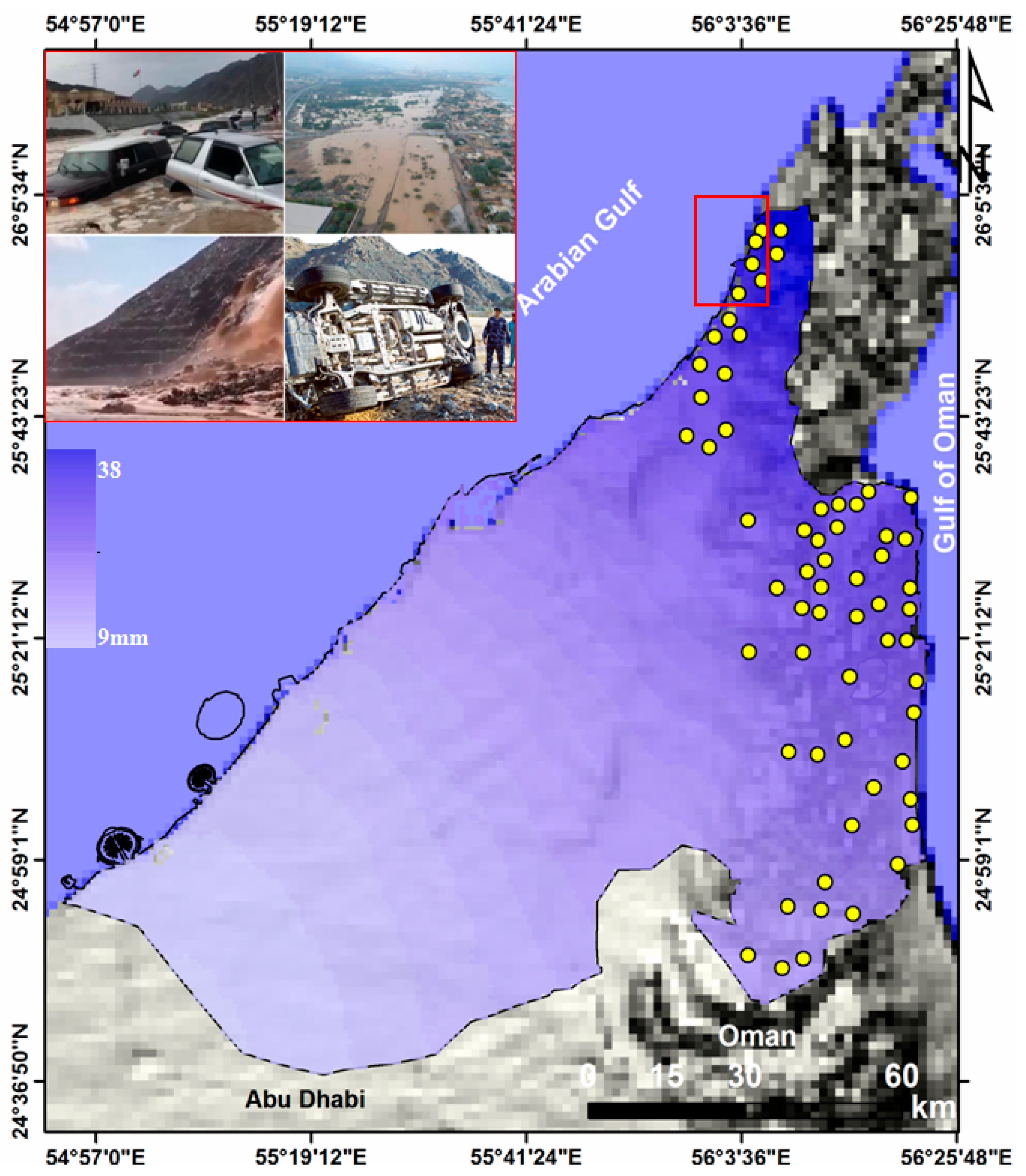
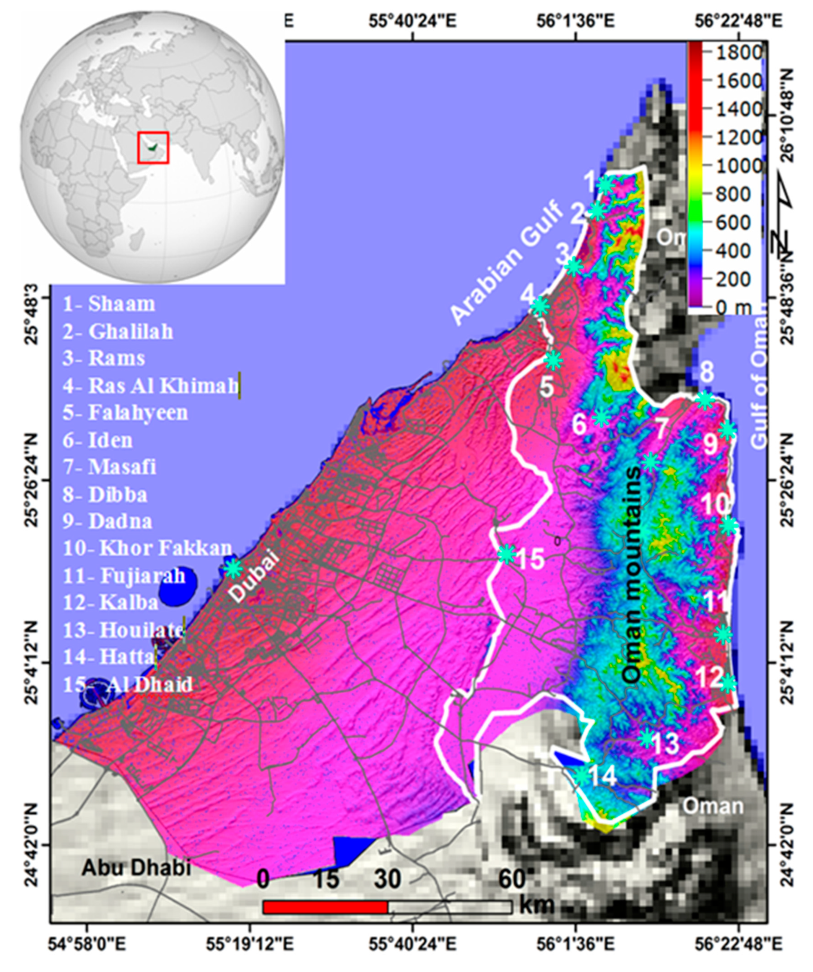
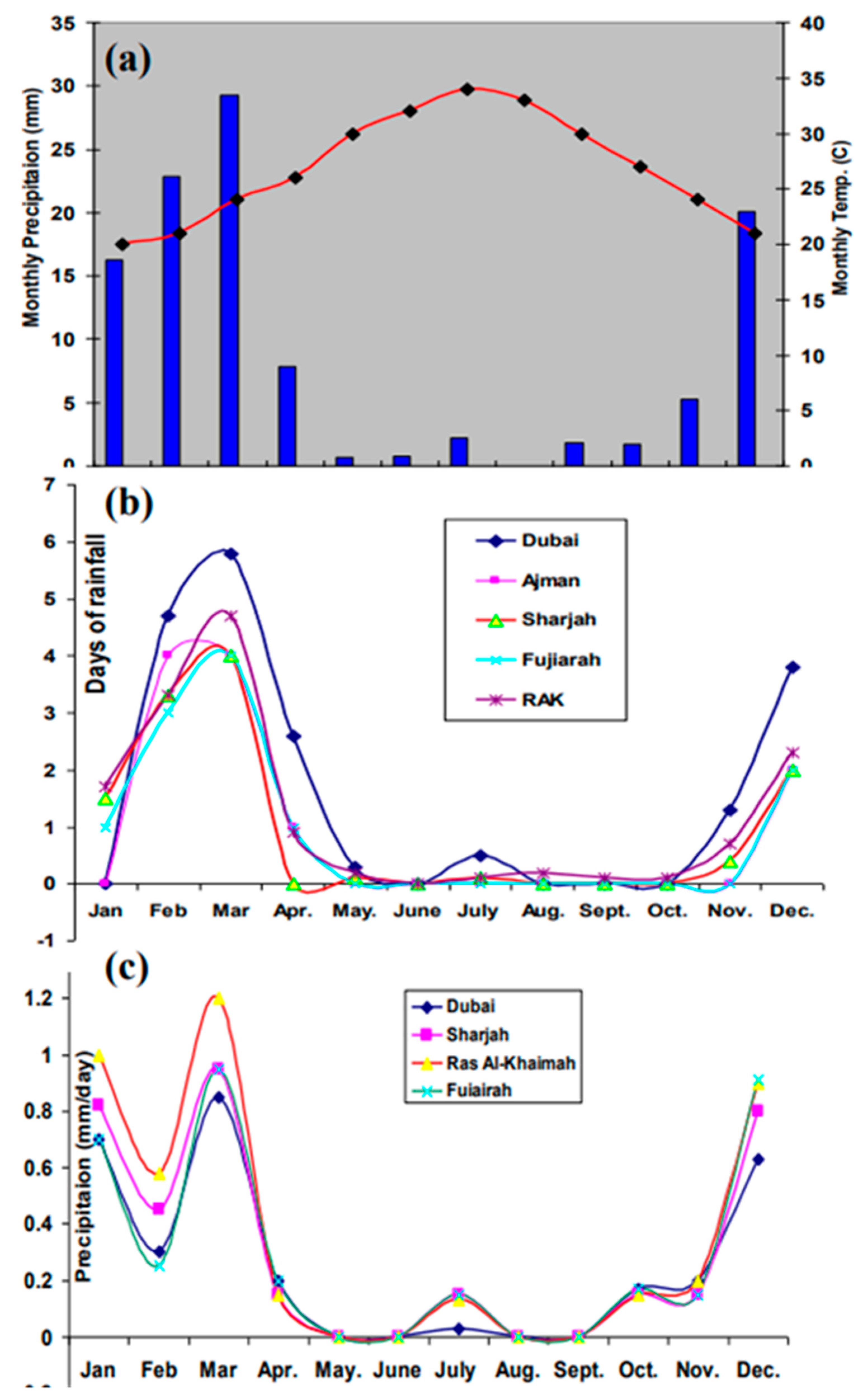
2. Study Area
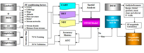
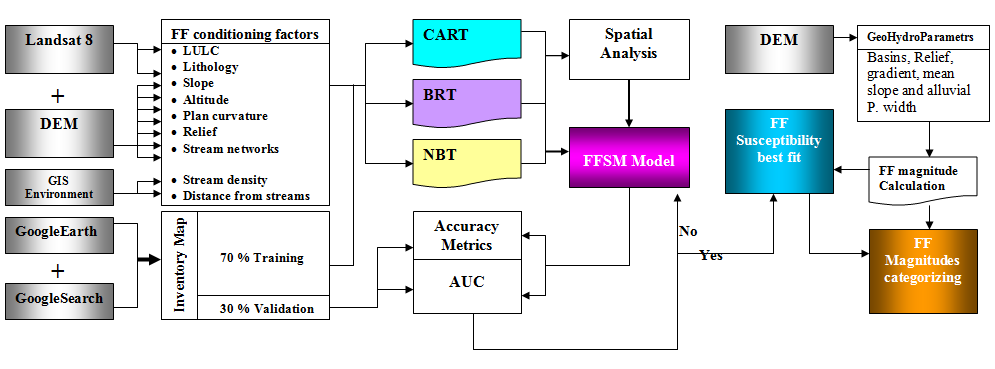
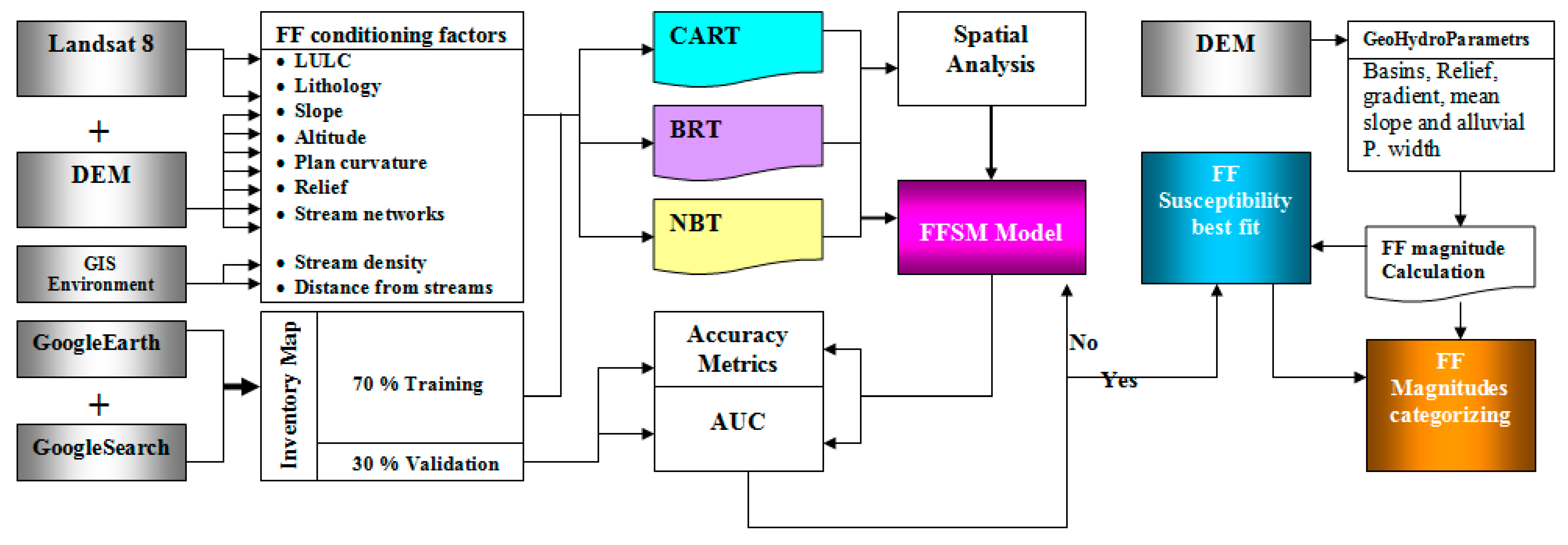
3. Datasets and Methodology
3.1. Construction of Flash Floods Inventory Map (FFIM)
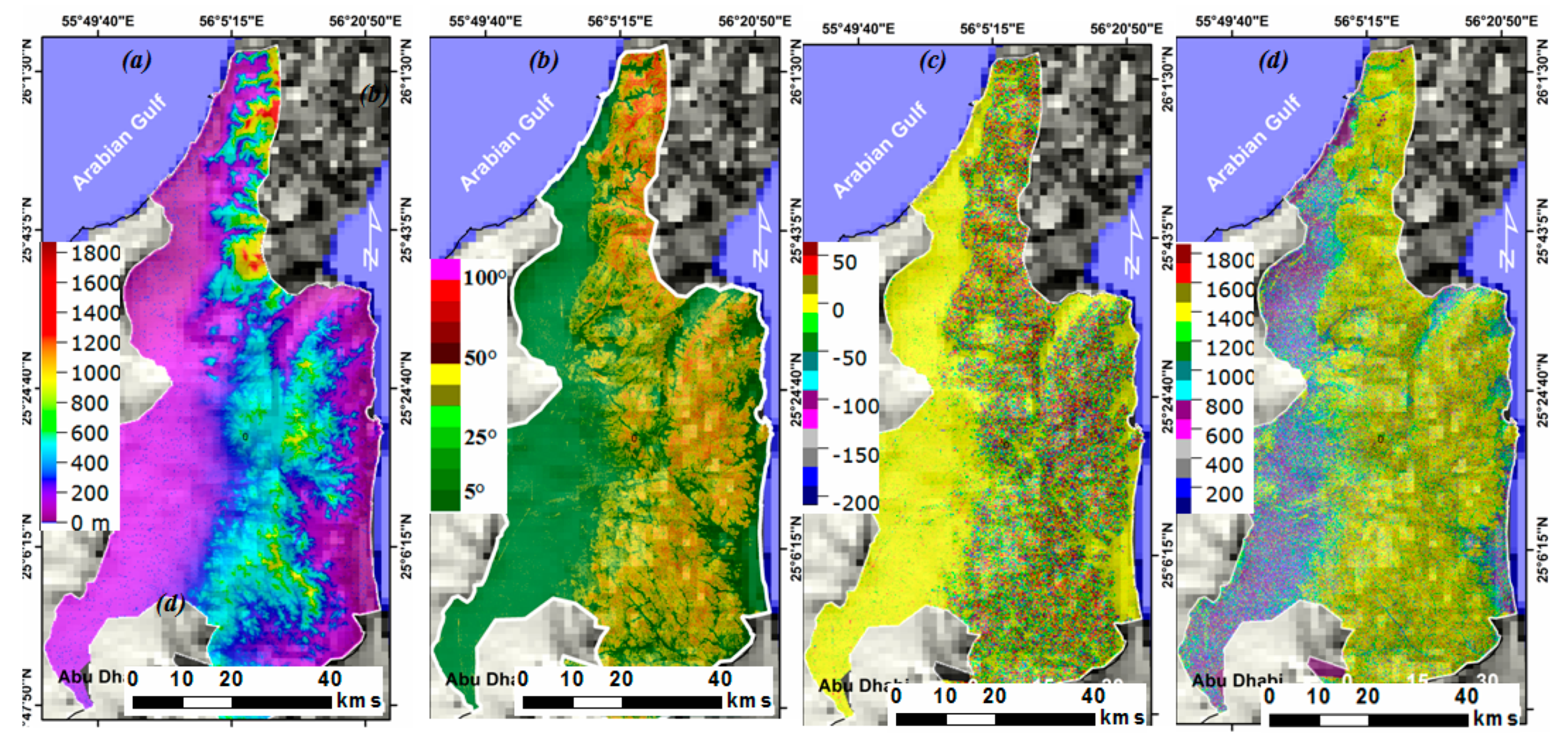
3.2. Spatial Analysis and Construction of Flash Flood Conditioning Parameters
3.2.1. Construction of FFCPs
3.2.2. Spatial Analysis
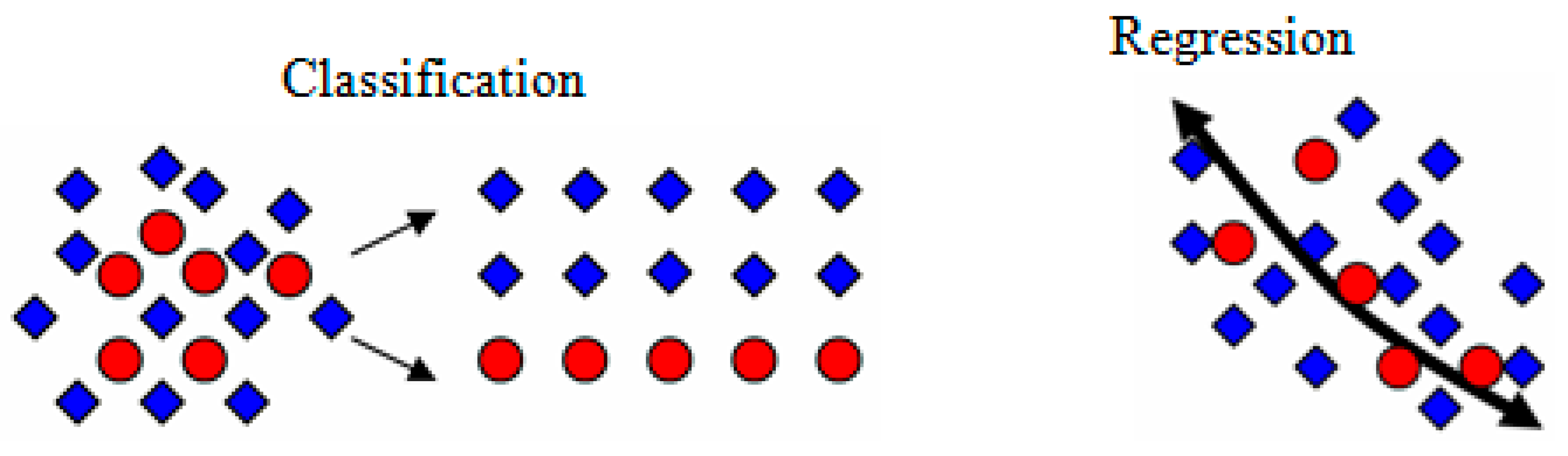
3.3. Background and Theories of Models
3.3.1. Boosted Regression Tree (BRT)
3.3.2. Classification and Regression Trees (CART)
3.3.3. Naive Bayes Tree (NBT)
3.4. Optimal Model Parameterisation and Flash Flood Susceptibility Mapping
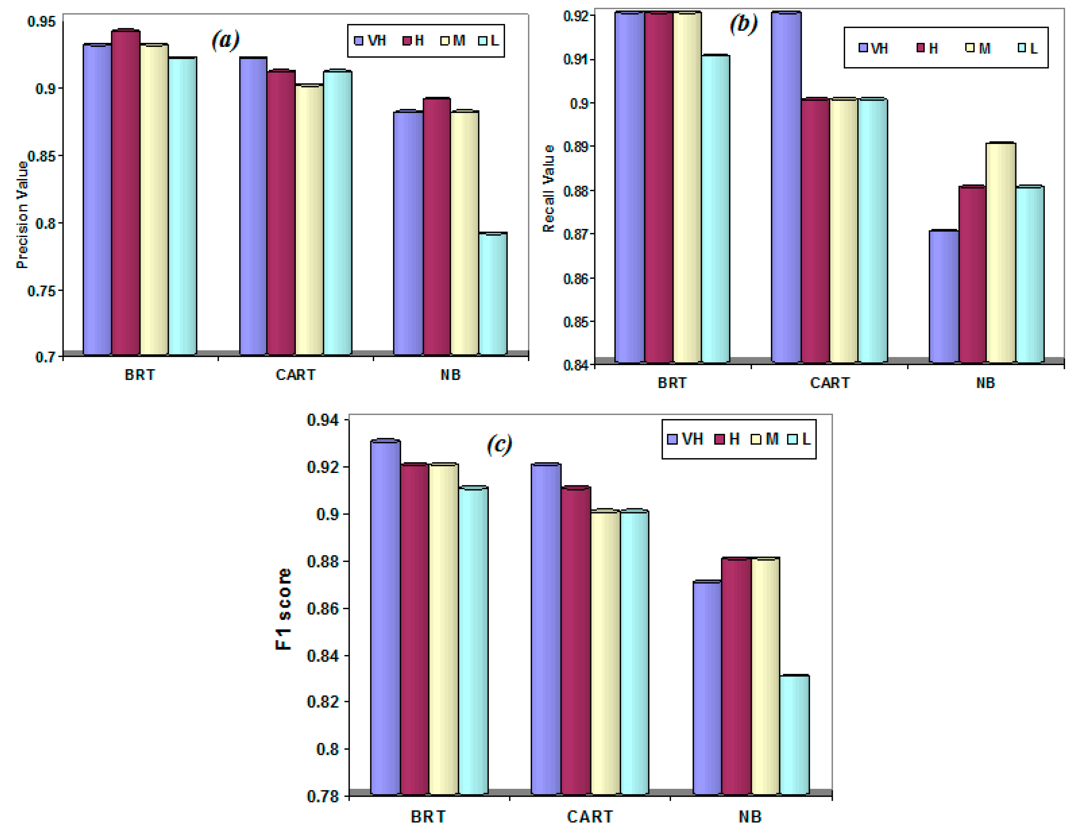
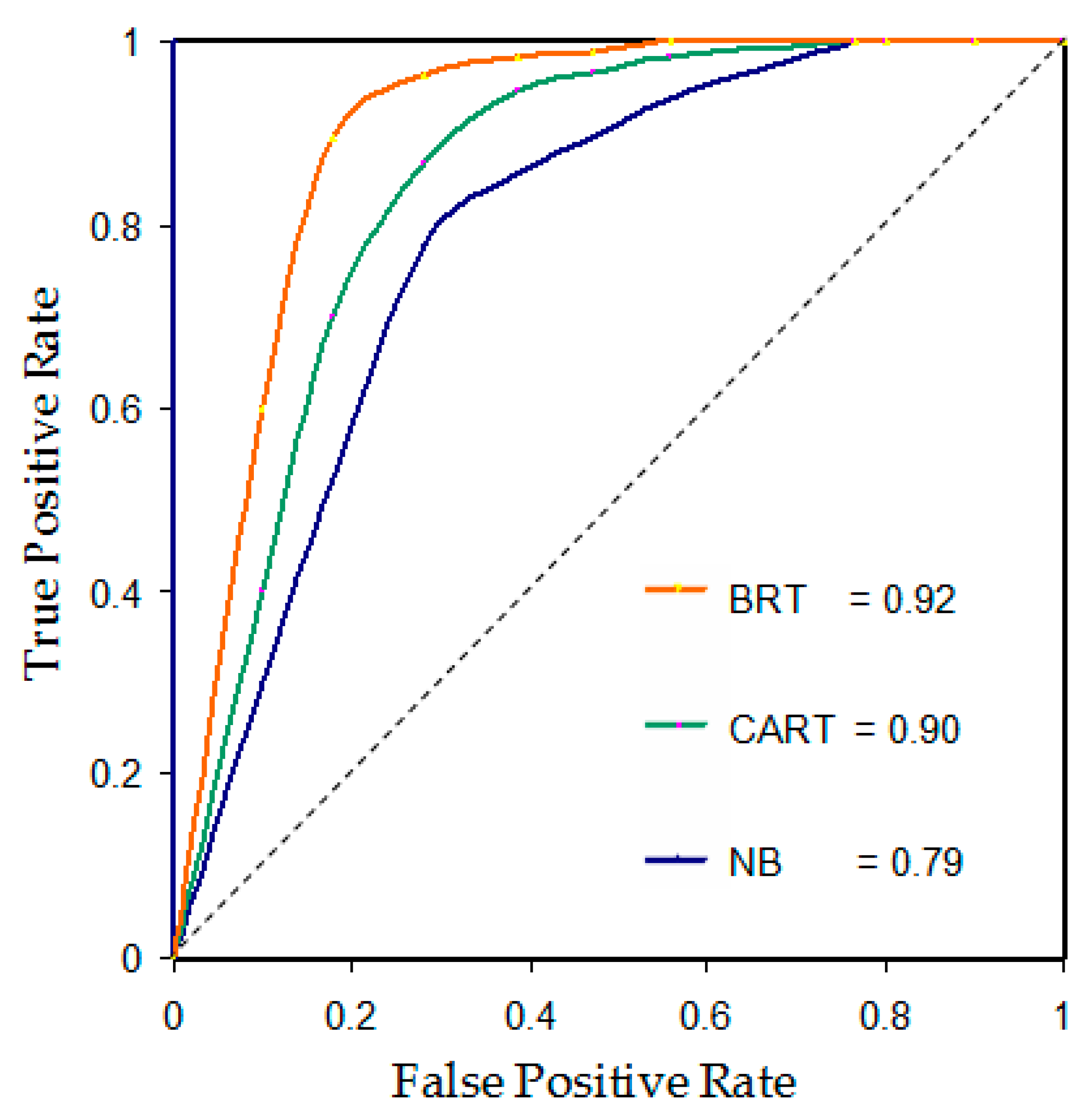
3.5. Evaluation of the Models Performance
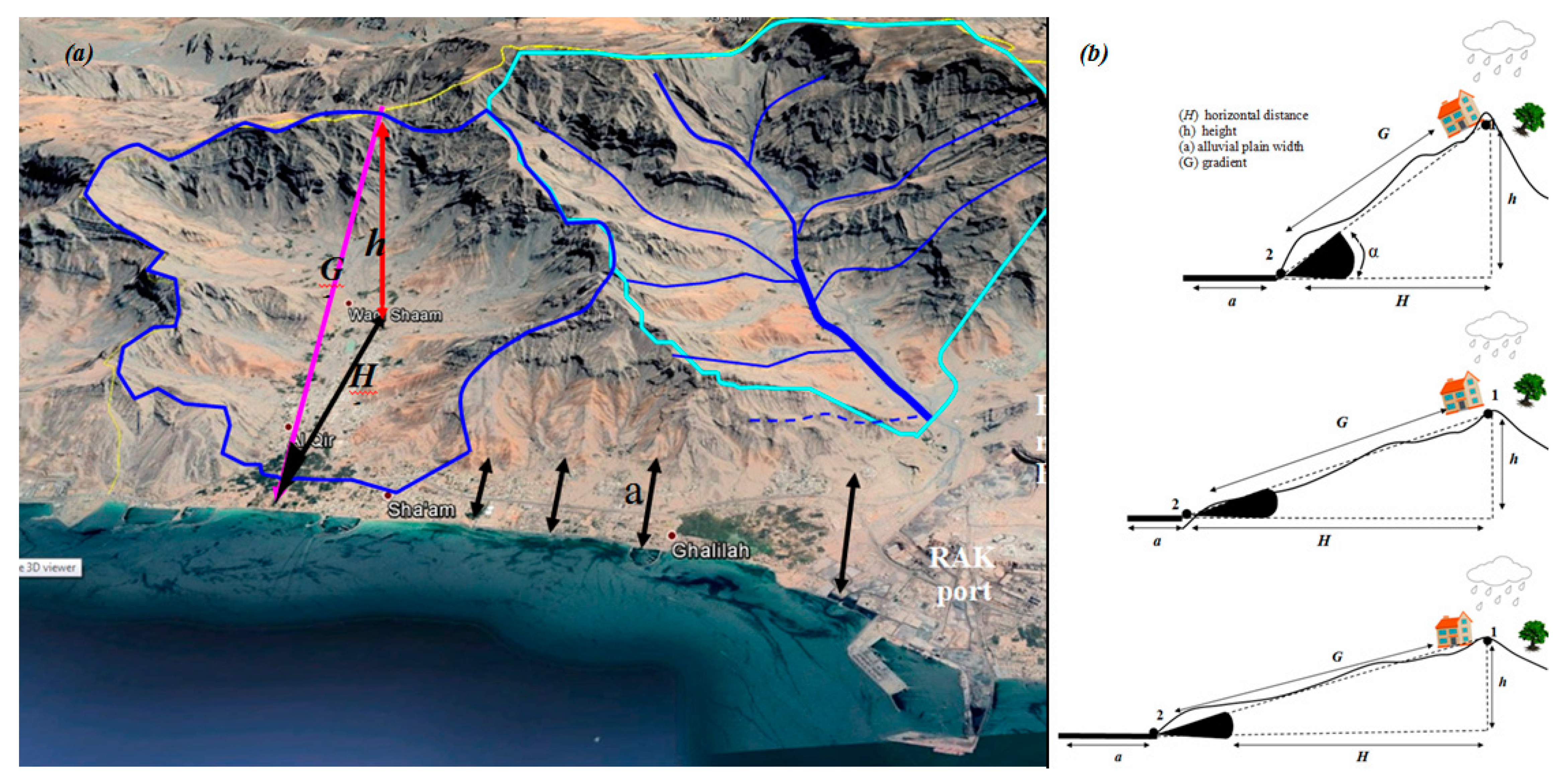
3.6. Geohydrological Model for FFMI and Filling the Gaps in MLC Maps
4. Results and Discussion
4.1. Evaluation of the Models Performance and Validation
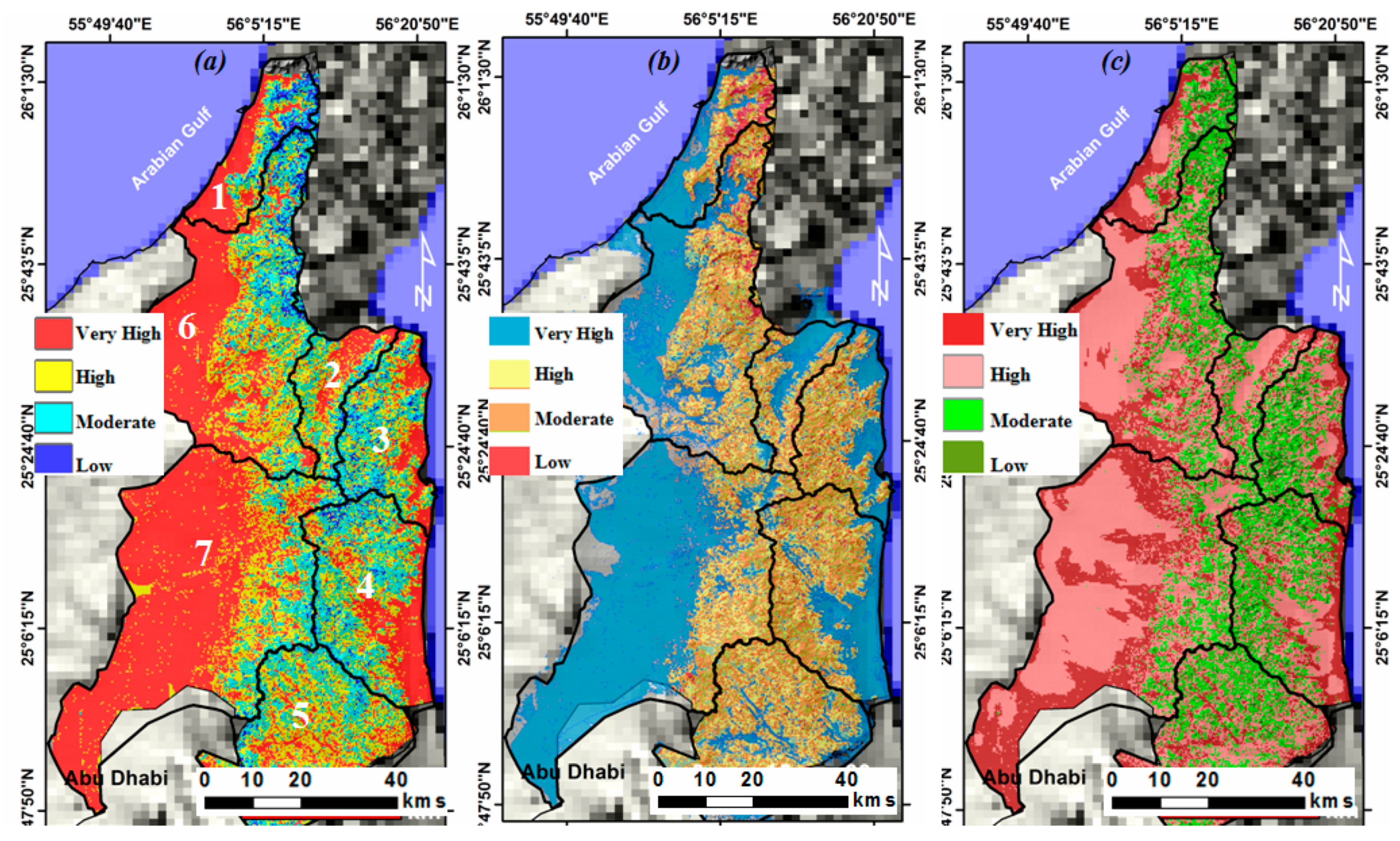
4.2. Spatial Analysis and Flash Floods Susceptibility Mapping
4.3. Geohydrological Model for FFMI and Filling the Gaps in MCL Maps
5. Discussion
5.1. Evaluation of the Models Performance and Validation
5.2. Spatial Analysis and Flash Floods Susceptibility Mapping
5.3. Geohydrological Model for FFM Indexing and Filling the Gaps in MLC Maps
6. Conclusions
Author Contributions
Funding
Acknowledgments
Conflicts of Interest
References
- Kron, W. Keynote lecture: Flood risk = hazard × exposure × vulnerability. In Flood Defence 2002; Science Press, New York Ltd.: New York, NY, USA, 2002; pp. 82–97. [Google Scholar]
- Yin, J.; Yu, D.; Yin, Z.; Liu, M.; He, Q. Evaluating the impact and risk of pluvial flash flood on intra-urban road network: A case study in the city center of Shanghai, China. J. Hydrol. 2016, 537, 138–145. [Google Scholar] [CrossRef] [Green Version]
- Casale, R.; Margottini, C. Floods and Landslides: Integrated Risk Assessment: Integrated Risk Assessment; with 30 Tables; Springer: Berlin/Heidelberg, Germany, 1999. [Google Scholar]
- Kohavi, R. Scaling up the accuracy of naive-bayes classifiers: A decision-tree hybrid. KDD 1996, 96, 202–207. [Google Scholar]
- Aksoy, H.; Kirca, V.S.O.; Burgan, H.I.; Kellecioglu, D. Hydrological and hydraulic models for determination of flood-prone and flood inundation areas. Proc. Int. Assoc. Hydrol. Sci. 2016, 373, 137–141. [Google Scholar] [CrossRef] [Green Version]
- Al-Hashemi, H.M.B.; Al-Amoudi, O.S.B. A review on the angle of repose of granular materials. Powder Technol. 2018, 330, 397–417. [Google Scholar] [CrossRef]
- Elkhrachy, I. Flash Flood Hazard Mapping Using Satellite Images and GIS Tools: A case study of Najran City, Kingdom of Saudi Arabia (KSA). Egypt. J. Remote Sens. Space Sci. 2015, 18, 261–278. [Google Scholar] [CrossRef] [Green Version]
- Elshorbagy, A.; Corzo, G.; Srinivasulu, S.; Solomatine, D.P. Experimental investigation of the predictive capabilities of data driven modeling techniques in hydrology—Part 2: Application. Hydrol. Earth Syst. Sci. 2010, 14, 1943–1961. [Google Scholar] [CrossRef] [Green Version]
- Folke, C. Resilience: The emergence of a perspective for social ecological systems analyses. Glob. Environ. Change 2006, 16, 253–267. [Google Scholar] [CrossRef]
- Santangelo, N.; Santo, A.; Di Crescenzo, G.; Foscari, G.; Liuzza, V.; Sciarrotta, S.; Scorpio, V. Flood susceptibility assessment in a highly urbanized alluvial fan: The case study of Sala Consilina (southern Italy). Nat. Hazards Earth Syst. Sci. 2011, 11, 2765–2780. [Google Scholar] [CrossRef] [Green Version]
- Wang, Y.; Hong, H.; Pourghasemi, H.R.; Li, S.; Pamucar, D.; Gigović, L.; Drobnjak, S.; Bui, D.T.; Duan, H. A Hybrid GIS Multi-Criteria Decision-Making Method for Flood Susceptibility Mapping at Shangyou, China. Remote Sens. 2018, 11, 62. [Google Scholar] [CrossRef] [Green Version]
- Elmahdy, S.I.; Mohamed, M.M.; Ali, T.A.; Abdalla, J.E.-D.; Abouleish, M. Land subsidence and sinkholes susceptibility mapping and analysis using random forest and frequency ratio models in Al Ain, UAE. Geocarto Int. 2020, 2020, 1–17. [Google Scholar] [CrossRef]
- Elmahdy, S.I.; Mohamed, M.M.; Ali, T. Land Use/Land Cover Changes Impact on Groundwater Level and Quality in the Northern Part of the United Arab Emirates. Remote Sens. 2020, 12, 1715. [Google Scholar] [CrossRef]
- Elmahdy, S.I.; Ali, T.A.; Mohamed, M.M.; Howari, F.M.; Abouleish, M.; Simonet, D. Spatiotemporal Mapping and Monitoring of Mangrove Forests Changes From 1990 to 2019 in the Northern Emirates, UAE Using Random Forest, Kernel Logistic Regression and Naive Bayes Tree Models. Front. Environ. Sci. 2020, 8, 102. [Google Scholar] [CrossRef]
- Quinn, P.; Beven, K.; Chevallier, P.; Planchon, O. The prediction of hillslope fow paths for distributed hydrological modeling using digital terrain models. Hydrol. Process. 1991, 5, 59–79. [Google Scholar] [CrossRef]
- Fortin, J.P.; Turcotte, R.; Massicotte, S.; Moussa, R.; Fritzback, J.; Villeneuve, J.P. Distributed watershed model compatible with remote sensing and GIS data, I: Description of model. J. Hydrol. Eng. 2001, 6, 91–99. [Google Scholar] [CrossRef]
- Jayakrishnan, R.; Srinivasan, R.; Santhi, C.; Arnold, J.G. Advances in the application of the SWAT model for water resources management. Hydrol. Process. 2005, 19, 749–762. [Google Scholar] [CrossRef]
- Bahremand, A.; De Smedt, F.; Corluy, J.; Liu, Y.B.; Poórová, J.; Velcická, L.; Kunikova, E.; Smedt, F. WetSpa Model Application for Assessing Reforestation Impacts on Floods in Margecany–Hornad Watershed, Slovakia. Water Resour. Manag. 2006, 21, 1373–1391. [Google Scholar] [CrossRef]
- Fenicia, F.; Kavetski, D.; Savenije, H.H.G.; Clark, M.P.; Schoups, G.; Pfister, L.; Freer, J. Catchment properties, function, and conceptual model representation: Is there a correspondence? Hydrol. Process. 2014, 28, 2451–2467. [Google Scholar] [CrossRef]
- Smith, D.I.; Ward, R. Floods: Physical Processes and Human Impacts; John Wiley and Sons Ltd.: Chichester, UK, 1998. [Google Scholar]
- Toth, E.; Brath, A.; Montanari, A. Comparison of short-term rainfall prediction models for real-time flood forecasting. J. Hydrol. 2000, 239, 132–147. [Google Scholar] [CrossRef]
- Şarlak, N. Flood Frequency Estimator with Nonparametric Approaches in Turkey. Fresenius Environ. Bull. 2012, 21, 1083–1089. [Google Scholar]
- Dou, J.; Shirzadi, A.; Ghaderi, K.; Omidavr, E.; Al-Ansari, N.; Clague, J.J.; Geertsema, M.; Khosravi, K.; Amini, A.; Bahrami, S.; et al. Flood Detection and Susceptibility Mapping Using Sentinel-1 Remote Sensing Data and a Machine Learning Approach: Hybrid Intelligence of Bagging Ensemble Based on K-Nearest Neighbor Classifier. Remote Sens. 2020, 12, 266. [Google Scholar] [CrossRef] [Green Version]
- Yalcin, A.; Yalçın, A. GIS-based landslide susceptibility mapping using analytical hierarchy process and bivariate statistics in Ardesen (Turkey): Comparisons of results and confirmations. Catena 2008, 72, 1–12. [Google Scholar] [CrossRef]
- Elmahdy, S.I.; Mohamed, M.M. Probabilistic frequency ratio model for groundwater potential mapping in Al Jaww plain, UAE. Arab. J. Geosci. 2015, 8, 2405–2416. [Google Scholar] [CrossRef]
- Bui, D.T.; Tsangaratos, P.; Ngo, P.T.; Pham, T.D.; Pham, B.T. Flash flood susceptibility modeling using an optimized fuzzy rule based feature selection technique and tree based ensemble methods . Sci. Total Environ. 2019, 668, 1038–1054. [Google Scholar] [CrossRef] [PubMed]
- Mohammady, M.; Pourghasemi, H.R.; Amiri, M. Assessment of land subsidence susceptibility in Semnan plain (Iran): A comparison of support vector machine and weights of evidence data mining algorithms. Nat. Hazards 2019, 99, 951–971. [Google Scholar] [CrossRef]
- Bui, D.T.; Hoang, N.-D.; Pijush, S. Spatial pattern analysis and prediction of forest fire using new machine learning approach of Multivariate Adaptive Regression Splines and Differential Flower Pollination optimization: A case study at Lao Cai province (Viet Nam). J. Environ. Manag. 2019, 237, 476–487. [Google Scholar] [CrossRef]
- Rahmati, O.; Pourghasemi, H.R.; Zeinivand, H. Flood susceptibility mapping using frequency ratio and weights-of-evidence models in the Golastan Province, Iran. Geocarto Int. 2015, 31, 42–70. [Google Scholar] [CrossRef]
- Khosravi, K.; Pham, B.T.; Chapi, K.; Shirzadi, A.; Dou, J.; Revhaug, I.; Prakash, I.; Bui, D.T. A comparative assessment of decision trees algorithms for flash flood susceptibility modeling at Haraz watershed, northern Iran. Sci. Total. Environ. 2018, 627, 744–755. [Google Scholar] [CrossRef]
- Zhao, G.; Pang, B.; Xu, Z.; Yue, J.; Tu, T. Mapping flood susceptibility in mountainous areas on a national scale in China. Sci. Total Environ. 2018, 615, 1133–1142. [Google Scholar] [CrossRef]
- Bui, D.T.; Ngo, P.-T.T.; Pham, T.D.; Jaafari, A.; Minh, N.Q.; Hoa, P.V.; Samui, P. A novel hybrid approach based on a swarm intelligence optimized extreme learning machine for flash flood susceptibility mapping. Catena 2019, 179, 184–196. [Google Scholar] [CrossRef]
- Bui, D.T.; Hoang, N.-D.; Martínez-Álvarez, F.; Ngo, P.-T.T.; Hoa, P.V.; Pham, T.D.; Samui, P.; Costache, R. A novel deep learning neural network approach for predicting flash flood susceptibility: A case study at a high frequency tropical storm area. Sci. Total Environ. 2020, 701, 134413. [Google Scholar] [CrossRef]
- Chen, X.; Ahmadi, M.H.; Busari, A. A comparative study of population-based optimization algorithms for downstream river flow forecasting by a hybrid neural network model. Eng. Appl. Artif. Intell. 2015, 46, 258–268. [Google Scholar] [CrossRef]
- Tsangaratos, P.; Ilia, I. Comparison of a logistic regression and Naïve Bayes classifier in landslide susceptibility assessments: The influence of models complexity and training dataset size. Catena 2016, 145, 164–179. [Google Scholar] [CrossRef]
- Khosravi, K.; Pourghasemi, H.R.; Chapi, K.; Bahri, M. Flash flood susceptibility analysis and its mapping using different bivariate models in Iran: A comparison between Shannon’s entropy, statistical index, and weighting factor models. Environ. Monit. Assess. 2016, 188, 656. [Google Scholar] [CrossRef] [PubMed]
- Al-Rashed, M.F.; Sherif, M.M. Water Resources in the GCC Countries: An Overview. Water Resour. Manag. 2000, 14, 59–75. [Google Scholar] [CrossRef]
- Sherif, M.; Almulla, M.; Shetty, A.; Chowdhury, R. Analysis of rainfall, PMP and drought in the United Arab Emirates. Int. J. Clim. 2014, 34, 1318–1328. [Google Scholar] [CrossRef]
- Giri, S.; Singh, A.K. Human health risk assessment via drinking water pathway due to metal contamination in the groundwater of Subarnarekha River Basin, India. Environ. Monit. Assess. 2015, 187, 63. [Google Scholar] [CrossRef] [PubMed]
- The Master Plan Study on the Groundwater Resources Development for Agriculture in the Vicinity of Al Dhaid in the UAE; Final Report; JICA International Cooperation Agency: Tokyo, Japan, 1996.
- Bui, D.T.; Tuan, T.A.; Klempe, H.; Pradhan, B.; Revhaug, I. Spatial prediction models for shallow landslide hazards: A comparative assessment of the efficacy of support vector machines, artificial neural networks, kernel logistic regression, and logistic model tree. Landslides 2015, 13, 361–378. [Google Scholar] [CrossRef]
- Pham, B.T.; Bui, D.T.; Dholakia, M.B.; Prakash, I.; Pham, H.V. A Comparative Study of Least Square Support Vector Machines and Multiclass Alternating Decision Trees for Spatial Prediction of Rainfall-Induced Landslides in a Tropical Cyclones Area. Geotech. Geol. Eng. 2016, 34, 1807–1824. [Google Scholar] [CrossRef]
- Fernández, D.; Lutz, M. Urban flood hazard zoning in Tucumán Province, Argentina, using GIS and multicriteria decision analysis. Eng. Geol. 2010, 111, 90–98. [Google Scholar] [CrossRef]
- Costache, R.; Pham, Q.B.; Sharifi, E.; Linh, N.T.; Abba, S.I.; Vojtek, M.; Khoi, D.N. Flash-flood susceptibility assessment using multi-criteria decision making and machine learning supported by remote sensing and gis techniques. Remote Sens. 2020, 12, 106. [Google Scholar] [CrossRef] [Green Version]
- Glenn, E.P.; Morino, K.; Nagler, P.L.; Murray, R.; Pearlstein, S.; Hultine, K.R. Roles of saltcedar (Tamarix spp.) and capillary rise in salinizing a non-flooding terrace on a flow-regulated desert river. J. Arid Environ. 2012, 79, 56–65. [Google Scholar] [CrossRef]
- Loosvelt, L.; Peters, J.; Skriver, H.; Lievens, H.; Van Coillie, F.M.; De Baets, B.; Verhoest, N.E.C. Random Forests as a tool for estimating uncertainty at pixel-level in SAR image classification. Int. J. Appl. Earth Obs. Geoinf. 2012, 19, 173–184. [Google Scholar] [CrossRef]
- Rahmati, O.; Pourghasemi, H.R.; Melesse, A.M. Application of GIS-based data driven random forest and maximum entropy models for groundwater potential mapping: A case study at Mehran Region, Iran. Catena 2015, 137, 360–372. [Google Scholar] [CrossRef]
- Santo, A.; Di Crescenzo, G.; Del Prete, S.; Di Iorio, L. The Ischia island flash flood of November 2009 (Italy): Phenomenon analysis and flood hazard. Phys. Chem. Earth 2012, 49, 3–17. [Google Scholar] [CrossRef]
- Nijzink, R.C.; Samaniego, L.; Mai, J.; Kumar, R.; Thober, S.; Zink, M.; Schafer, D.; Savenije, H.H.; Hrachowitz, M. The importance of topography-controlled sub-grid process heterogeneity and semi-quantitative prior constraints in distributed hydrological models. Hydrol. Earth Syst. Sci. 2016, 20, 1151–1176. [Google Scholar] [CrossRef] [Green Version]
- Schapire, R.E. The Boosting Approach to Machine Learning: An Overview. In Nonlinear Estimation and Classification; Springer: New York, NY, USA, 2003; pp. 149–171. [Google Scholar]
- Gordon, A.D.; Breiman, L.; Friedman, J.H.; Olshen, R.A.; Stone, C.J. Classification and Regression Trees. Biometrics 1984, 40, 874. [Google Scholar] [CrossRef] [Green Version]
- Chen, W.; Li, Y.; Tsangaratos, P.; Shahabi, H.; Ilia, I.; Xue, W.; Bian, H. Groundwater Spring Potential Mapping Using Artificial Intelligence Approach Based on Kernel Logistic Regression, Random Forest, and Alternating Decision Tree Models. Appl. Sci. 2020, 10, 425. [Google Scholar] [CrossRef] [Green Version]
- Elith, J.; Leathwick, J.R.; Hastie, T. A working guide to boosted regression trees. J. Anim. Ecol. 2008, 77, 802–813. [Google Scholar] [CrossRef]
- Rothwell, J.J.; Futter, M.; Dise, N.B. A classification and regression tree model of controls on dissolved inorganic nitrogen leaching from European forests. Environ. Pollut. 2008, 156, 544–552. [Google Scholar] [CrossRef]
- Friedman, L.A. The Measure of a Successful Information Storage and Retrieval System. In Perspectives in Information Science; Springer: Dordrect, The Netherlands, 1975; pp. 379–408. [Google Scholar]
- Breiman, L.; Jerome, F.; Charles, J.S.; Richard, A.O. Classification and Regression Trees; Wadsworth Int. Group: Dordrecht, The Netherlands, 1984; Volume 37, pp. 237–251. [Google Scholar]
- Breiman, L.; Stone, C.J. Parsimonious Binary Classification Trees; California Technical Report TSCCSD-TN; Technology Service Corporation: Santa Monica, CA, USA, 1978; Volume 4. [Google Scholar]
- Türe, M.; Tokatli, F.; Kurt, I.; Tokatlı, F. Using Kaplan–Meier analysis together with decision tree methods (C&RT, CHAID, QUEST, C4.5 and ID3) in determining recurrence-free survival of breast cancer patients. Expert Syst. Appl. 2009, 36, 2017–2026. [Google Scholar] [CrossRef]
- Chang, C.C.; Lin, C.J. LIBSVM: A library for support vector machines. TIST 2011, 2, 1–27. [Google Scholar] [CrossRef]
- Yang, L.; Xian, G.; Klaver, J.M.; Deal, B. Urban Land-Cover Change Detection through Sub-Pixel Imperviousness Mapping Using Remotely Sensed Data. Photogramm. Eng. Remote Sens. 2003, 69, 1003–1010. [Google Scholar] [CrossRef]
- Smeti, E.M.; Thanasoulias, N.; Lytras, E.; Tzoumerkas, P.; Golfinopoulos, S. Treated water quality assurance and description of distribution networks by multivariate chemometrics. Water Res. 2009, 43, 4676–4684. [Google Scholar] [CrossRef] [PubMed]
- Hazir, M.H.M.; Shariff, A.; Amiruddin, M.D.; Ramli, A.R.; Saripan, M.I. Oil palm bunch ripeness classification using fluorescence technique. J. Food Eng. 2012, 113, 534–540. [Google Scholar] [CrossRef]
- Chudzinska, M.; Barałkiewicz, D. Application of ICP-MS method of determination of 15 elements in honey with chemometric approach for the verification of their authenticity. Food Chem. Toxicol. 2011, 49, 2741–2749. [Google Scholar] [CrossRef]
- Vorpahl, P.; Elsenbeer, H.; Märker, M.; Schröder, B.; Maerker, M. How can statistical models help to determine driving factors of landslides? Ecol. Model. 2012, 239, 27–39. [Google Scholar] [CrossRef]
- Naghibi, S.A.; Pourghasemi, H.R.; Dixon, B. GIS-based groundwater potential mapping using boosted regression tree, classification and regression tree, and random forest machine learning models in Iran. Environ. Monit. Assess. 2016, 188, 1–27. [Google Scholar] [CrossRef]
- Taha, M.M.; Elbarbary, S.M.; Naguib, D.M.; El-Shamy, I.Z. Flash flood hazard zonation based on basin morphometry using remote sensing and GIS techniques: A case study of Wadi Qena basin, Eastern Desert, Egypt. Remote Sens Appl Soc Environ. 2017, 8, 157–167. [Google Scholar] [CrossRef]
- Liang, L.; Lu, Y.L.; Yang, H. Toxicology of isoproturon to the food crop wheat as affected by salicylic acid. Environ. Sci. Pollut. Res. 2012, 19, 2044–2054. [Google Scholar] [CrossRef]
- Townsend, P.A.; Walsh, S.J. Modeling floodplain inundation using an integrated GIS with radar and optical remote sensing. Geomorphology 1998, 21, 295–312. [Google Scholar] [CrossRef]
- Farid, D.M.; Zhang, L.; Rahman, C.M.; Hossain, M.A.; Strachan, R. Hybrid decision tree and naïve Bayes classifiers for multi-class classification tasks. Expert Syst. Appl. 2014, 41, 1937–1946. [Google Scholar] [CrossRef]
- Pham, T.P.T.; Kaushik, R.; Parshetti, G.K.; Mahmood, R.; Balasubramanian, R. Food waste-to-energy conversion technologies: Current status and future directions. Waste Manag. 2015, 38, 399–408. [Google Scholar] [CrossRef] [PubMed]
- Ho, T.K. The random subspace method for constructing decision forests. IEEE Trans. Pattern Anal. Mach. Intell. 1998, 20, 832–844. [Google Scholar] [CrossRef] [Green Version]
- Wang, W.-C.; Ahmadi, M.H.; Xu, D.-M.; Chen, X.-Y. Improving Forecasting Accuracy of Annual Runoff Time Series Using ARIMA Based on EEMD Decomposition. Water Resour. Manag. 2015, 29, 2655–2675. [Google Scholar] [CrossRef]
- Hill, T.; Lewicki, P. Statistics: Methods and Applications: A Comprehensive Reference for Science, Industry and Data Mining; StatSoft, Inc.: Tulsa, OK, USA, 2006. [Google Scholar]
- Friedman, J.H. Greedy function approximation: A gradient boosting machine. Ann. Stat. 2001, 29, 1189–1232. [Google Scholar] [CrossRef]
- Friedman, J.H. Stochastic gradient boosting. Comput. Stat. Data Anal. 2002, 38, 367–378. [Google Scholar] [CrossRef]
- Venables, W.N.; Smith, D.M.; R Development Core Team. An Introduction to r. A Programming Environment for Data Analysis and Graphics; R Development Core Team: Vienna, Austria, 2006. [Google Scholar]
- Ridgeway, G. Gbm: Generalized Boosted Regression Models, R package, version 2.1.1; R Foundation for Statistical Computing: Vienna, Austria; Available online: http://CRAN.R-project.org/package=gbm (accessed on 21 March 2017).
- Ozdemir, A. GIS-based groundwater spring potential mapping in the Sultan Mountains (Konya, Turkey) using frequency ratio, weights of evidence and logistic regression methods and their comparison. J. Hydrol. 2011, 411, 290–308. [Google Scholar] [CrossRef]
- Ozdemir, A. Using a binary logistic regression method and GIS for evaluating and mapping the groundwater spring potential in the Sultan Mountains (Aksehir, Turkey). J. Hydrol. 2011, 405, 123–136. [Google Scholar] [CrossRef]
- Ha, N.T.; Manley-Harris, M.; Pham, T.D.; Hawes, I. A Comparative Assessment of Ensemble-Based Machine Learning and Maximum Likelihood Methods for Mapping Seagrass Using Sentinel-2 Imagery in Tauranga Harbor, New Zealand. Remote Sens. 2020, 12, 355. [Google Scholar] [CrossRef] [Green Version]
- Naghibi, S.A.; Pourghasemi, H.R. A Comparative Assessment Between Three Machine Learning Models and Their Performance Comparison by Bivariate and Multivariate Statistical Methods in Groundwater Potential Mapping. Water Resour. Manag. 2015, 29, 5217–5236. [Google Scholar] [CrossRef]
- Naghibi, S.A.; Pourghasemi, H.R.; Pourtaghi, Z.S.; Rezaei, A. Groundwater qanat potential mapping using frequency ratio and Shannon’s entropy models in the Moghan watershed, Iran. Earth Sci. Inform. 2015, 8, 171–186. [Google Scholar] [CrossRef]
- Rahmati, O.; Pourghasemi, H.R. Identification of critical flood prone areas in data-scarce and ungauged regions: A comparison of three data mining models. Water Resour. Manag. 2017, 31, 1473–1487. [Google Scholar] [CrossRef]
- Pourghasemi, H.R.; Xie, X.; Peng, J.B.; Dou, J.; Hong, H.; Bui, D.T.; Duan, Z.; Li, S.; Zhu, A.-X. GIS-based landslide susceptibility evaluation using a novel hybrid integration approach of bivariate statistical based random forest method. Catena 2018, 164, 135–149. [Google Scholar] [CrossRef]
- Nandi, A.; Shakoor, A. A GIS-based landslide susceptibility evaluation using bivariate and multivariate statistical analyses. Eng. Geol. 2009, 110, 11–20. [Google Scholar] [CrossRef]
- Hong, H.; Tsangaratos, P.; Ilia, I.; Liu, J.; Zhu, A.-X.; Chen, W. Application of fuzzy weight of evidence and data mining techniques in construction of flood susceptibility map of Poyang County, China. Sci. Total. Environ. 2018, 625, 575–588. [Google Scholar] [CrossRef]
- Shin, Y. Application of Boosting Regression Trees to Preliminary Cost Estimation in Building Construction Projects. Comput. Intell. Neurosci. 2015, 2015, 1–9. [Google Scholar] [CrossRef] [Green Version]
- Chauhan, S.; Sharma, M.; Arora, M.K. Landslide susceptibility zonation of the Chamoli region, Garhwal Himalayas, using logistic regression model. Landslides 2010, 7, 411–423. [Google Scholar] [CrossRef]
- Moisen, G.G.; Freeman, E.A.; Blackard, J.A.; Frescino, T.S.; Zimmermann, N.E.; Edwards, T.C. Predicting tree species presence and basal area in Utah: A comparison of stochastic gradient boosting, generalized additive models, and tree-based methods. Ecol. Model. 2006, 199, 176–187. [Google Scholar] [CrossRef]
- Osaragi, T. Classification Methods for Spatial Data Representation; Tokyo Institute of Technology: Tokyo, Japan, 2002. [Google Scholar]
- Green, J.I.; Nelson, E.J. Calculation of time of concentration for hydrologic design and analysis using geographic information system vector objects. J. Hydroinform. 2002, 4, 75–81. [Google Scholar] [CrossRef] [Green Version]
- Guisan, A.; Thuiller, W. Predicting species distribution: Offering more than simple habitat models. Ecol. Lett. 2005, 8, 993–1009. [Google Scholar] [CrossRef]
- Oliveira, S.; Oehler, F.; San-Miguel-Ayanz, J.; Camia, A.; Pereira, J. Modeling spatial patterns of fire occurrence in Mediterranean Europe using Multiple Regression and Random Forest. For. Ecol. Manag. 2012, 275, 117–129. [Google Scholar] [CrossRef]
- Rahmati, O.; Falah, F.; Dayal, K.S.; Deo, R.; Mohammadi, F.; Biggs, T.; Moghaddam, D.D.; Naghibi, S.A.; Bui, D.T. Machine learning approaches for spatial modeling of agricultural droughts in the south-east region of Queensland Australia. Sci. Total Environ. 2019, 699, 134230. [Google Scholar] [CrossRef] [PubMed]
- Martins, S.; Bernardo, N.M.R.; Ogashawara, I.; Alcântara, E. Support Vector Machine algorithm optimal parameterization for change detection mapping in Funil Hydroelectric Reservoir (Rio de Janeiro State, Brazil). Model. Earth Syst. Environ. 2016, 2, 138. [Google Scholar] [CrossRef] [Green Version]
- Bathrellos, G.; Skilodimou, H.D.; Chousianitis, K.; Youssef, A.M.; Pradhan, B. Suitability estimation for urban development using multi-hazard assessment map. Sci. Total Environ. 2017, 575, 119–134. [Google Scholar] [CrossRef] [PubMed]
- Chen, W.; Hong, H.; Li, S.; Shahabi, H.; Wang, Y.; Wang, X.; Bin Ahmad, B. Flood susceptibility modelling using novel hybrid approach of reduced-error pruning trees with bagging and random subspace ensembles. J. Hydrol. 2019, 575, 864–873. [Google Scholar] [CrossRef]


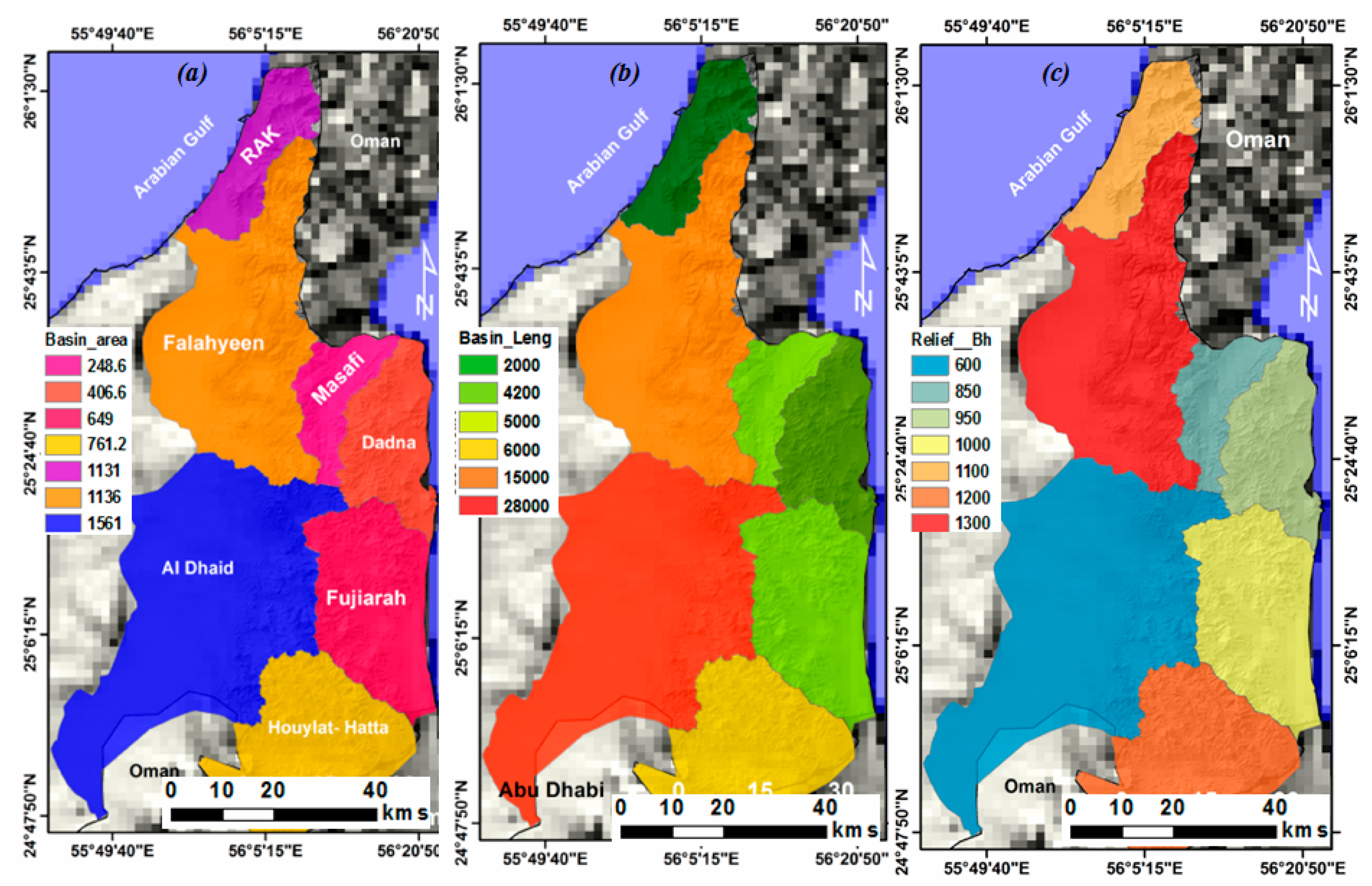
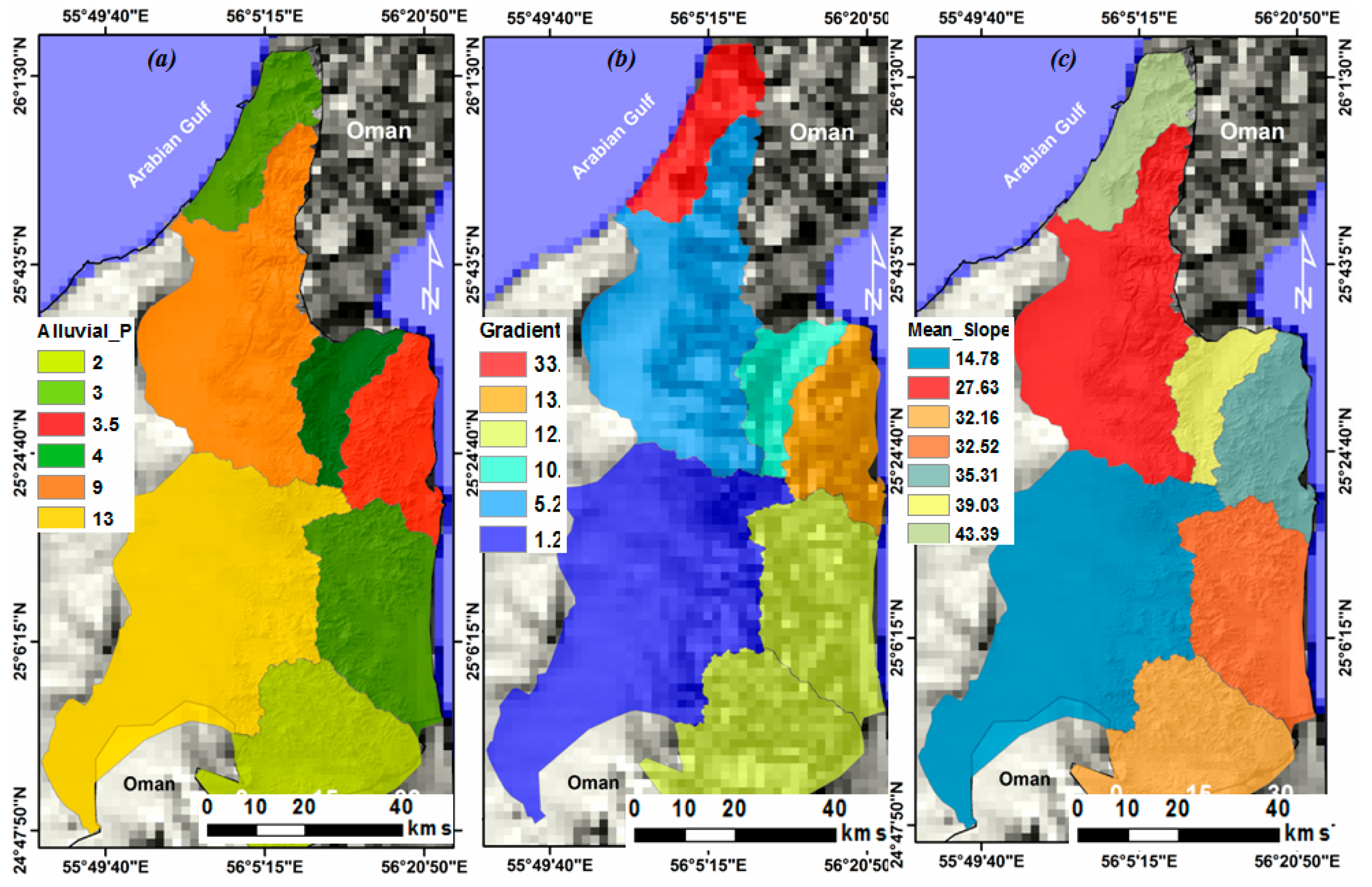
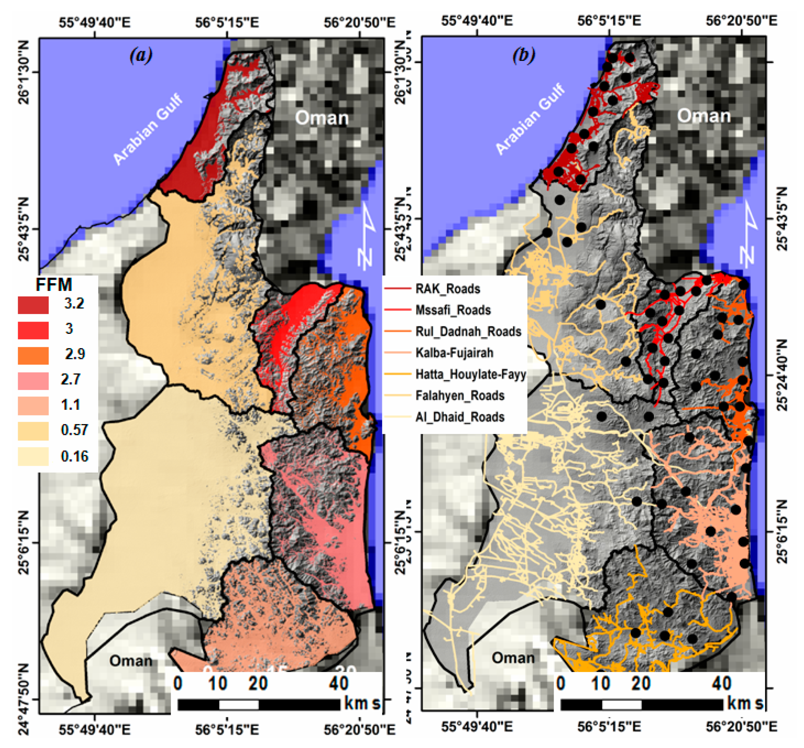
| Basin | Lb | Bh (m) | G° | A (km2) | Aw | MS | FFM |
|---|---|---|---|---|---|---|---|
| RAK | 2000 | 1100 | 33 | 1131 | 3 | 43.39 | 3.24 |
| Falaheyn | 15,000 | 1300 | 5.2 | 1136 | 9 | 27.63 | 0.57 |
| Al Dhaid | 28,000 | 600 | 1.28 | 1561 | 13 | 14.78 | 0.16 |
| Masafi | 5000 | 850 | 10.2 | 248.6 | 4 | 39.03 | 3 |
| Rul Dadnah-Dibba | 4200 | 950 | 13.5 | 406.6 | 3.5 | 35.31 | 2.96 |
| Fujiarah-Kalba | 5000 | 1000 | 12 | 649 | 3 | 32.52 | 2.71 |
| Hatta-Houylate | 6000 | 1200 | 12 | 761.2 | 2 | 32.16 | 1.11 |
| Total | 5893.4 |
© 2020 by the authors. Licensee MDPI, Basel, Switzerland. This article is an open access article distributed under the terms and conditions of the Creative Commons Attribution (CC BY) license (http://creativecommons.org/licenses/by/4.0/).
Share and Cite
Elmahdy, S.; Ali, T.; Mohamed, M. Flash Flood Susceptibility Modeling and Magnitude Index Using Machine Learning and Geohydrological Models: A Modified Hybrid Approach. Remote Sens. 2020, 12, 2695. https://0-doi-org.brum.beds.ac.uk/10.3390/rs12172695
Elmahdy S, Ali T, Mohamed M. Flash Flood Susceptibility Modeling and Magnitude Index Using Machine Learning and Geohydrological Models: A Modified Hybrid Approach. Remote Sensing. 2020; 12(17):2695. https://0-doi-org.brum.beds.ac.uk/10.3390/rs12172695
Chicago/Turabian StyleElmahdy, Samy, Tarig Ali, and Mohamed Mohamed. 2020. "Flash Flood Susceptibility Modeling and Magnitude Index Using Machine Learning and Geohydrological Models: A Modified Hybrid Approach" Remote Sensing 12, no. 17: 2695. https://0-doi-org.brum.beds.ac.uk/10.3390/rs12172695